In this paper we study gapless fermionic and bosonic systems in $d$-dimensional continuum space with $U(1)$ particle-number conservation and $\mathbb{R}^{d}$ translation symmetry. We write down low energy effective field theories for several gapless phases where $U(1)\times\mathbb{R}^{d}$ is viewed as internal symmetry. The $U(1)\times\mathbb{R}^{d}$ symmetry, when viewed as an internal symmetry, has a mixed anomaly, and the different effective field theories for different phases must have the same mixed anomaly. Such a mixed anomaly is proportional to the particle number density, and can be measured from the distribution of the total momentum $\boldsymbol{k}_{\text{tot}}$ for low energy many-body states (i.e. how such a distribution is shifted by $U(1)$ symmetry twist $\boldsymbol{a}$), as well as some other low energy universal properties of the systems. In particular, we write down low energy effective field theory for Fermi liquid with infinite number of fields, in the presence of both real space magnetic field and $\boldsymbol{k}$-space “magnetic” field. The effective field theory also captures the mixed anomaly, which constraints the low energy dynamics, such as determine the volume of Fermi surface (which is another formulation of Luttinger-Ward-Oshikawa theorem).

Low energy effective field theories of fermion liquids and mixed $U(1)\times\mathbb{R}^{d}$ anomaly

I Introduction

A gapless Fermi liquid for spinless fermions in $d$-dimensional space is described by the following integrated Boltzmann equation (if we ignore the collision term that is irrelevant under the renormalization group scaling) Kim et al. (1995)

$$\partial_{t}u(\boldsymbol{x},\boldsymbol{k}_{F},t)+\partial_{\boldsymbol{x}}\cdot\big{(}\boldsymbol{v}_{F}(\boldsymbol{k}_{F})u(\boldsymbol{x},\boldsymbol{k}_{F},t)\big{)}$$

$$+\partial_{\boldsymbol{k}_{F}}\cdot\big{(}\boldsymbol{f}(\boldsymbol{x})u(\boldsymbol{x},\boldsymbol{k}_{F},t)\big{)}=0,$$ (1)

where $\boldsymbol{k}_{F}$ parametrizes the Fermi surface, $\boldsymbol{v}_{F}$ is the Fermi velocity, $u(\boldsymbol{x},\boldsymbol{k}_{F})$ describes the Fermi surface displacement at Fermi momentum $\boldsymbol{k}_{F}$ and spacial location $\boldsymbol{x}$, and $\boldsymbol{f}$ is the force acting on a fermion. We can view the integrated Boltzmann equation as the equation of motion for the bosonized Fermi liquid.Luther (1979); Haldane (1992); Houghton and Marston (1993); Castro Neto and Fradkin (1994) Together with the total energy (assuming $\boldsymbol{f}=0$)

$$E=\int\hskip 1.0pt\mathrm{d}^{d}\boldsymbol{x}\frac{\hskip 1.0pt\mathrm{d}^{d-1}\boldsymbol{k}_{F}}{(2\pi)^{d}}\,\frac{|\boldsymbol{v}_{F}(\boldsymbol{k}_{F})|}{2}u^{2}(\boldsymbol{x},\boldsymbol{k}_{F}),$$ (2)

we obtain a phase-space low energy effective Lagrangian for Fermi liquid (see eqn. (IV.1)). Note that the low energy effective field theory contain infinite number of fields labeled by $\boldsymbol{k}_{F}$. Or alternatively, the low energy effective field theory can be viewed as having a single scaler field in $(d+d-1)$-dimensional space, but the interaction in the $d-1$ dimensions (parametrized by $\boldsymbol{k}_{F}$) is allowed to be non-local.

However, such a low energy effective theory fails to capture one of the most important properties of Fermi liquid: the volume enclosed by the Fermi surface is $(2\pi)^{d}\bar{\rho}$ where $\bar{\rho}$ is the density of the fermion in the ground state,Luttinger and Ward (1960); Oshikawa (2000) since the fermion density $\bar{\rho}$ does not even appear in the above formulation.

In recent years, it was realized that the Lieb-Schultz-Mattis (LSM) theoremLieb et al. (1961) and its higher-dimensional generalizations by OshikawaOshikawa (2000) and HastingsHastings (2004) can be understood in term of a mixed anomaly between translation symmetry and an internal symmetry.Furuya and Oshikawa (2017); Cheng et al. (2016); Po et al. (2017); Lu et al. (2020); Lu (2017); Cheng (2019); Jiang et al. (2019) For a 1-dimensional system with $U(1)$ symmetry and translation symmetry, there is a similar LSM theorem when the $U(1)$ charge per site is not an integer.Chen et al. (2011) This suggests that such a system also has a mixed anomaly when the $U(1)$ charge per site is not an integer. Similarly, for continuum systems with $U(1)$ and translation $\mathbb{R}^{d}$ symmetries, there should also be a mixed anomaly, whenever the $U(1)$ charge density is non-zero.

The low energy effective field theory for systems with $U(1)\times\mathbb{R}^{d}$ symmetry should capture this mixed $U(1)\times\mathbb{R}^{d}$ anomaly. Here we like to remark that the $U(1)\times\mathbb{R}^{d}$ symmetry is an exact symmetry. In the low energy effective field theory, $U(1)\times\mathbb{R}^{d}$ can be viewed as an internal symmetry. But when viewed as an internal symmetry, $U(1)\times\mathbb{R}^{d}$ may have a mixed anomaly, and this is the so called mixed anomaly discussed in this paper and in Ref. Furuya and Oshikawa, 2017; Cheng et al., 2016; Po et al., 2017; Lu et al., 2020; Lu, 2017; Cheng, 2019; Jiang et al., 2019

The Fermi liquid at low energies also has many emergent symmetries. In particular, the $U(1)$ fermion-number-conservation symmetry is enlarged to $U^{\infty}(1)$ emergent symmetry.Luther (1979); Haldane (1992); Houghton and Marston (1993); Castro Neto and Fradkin (1994) Recently, it was pointed out that such an emergent $U^{\infty}(1)$ symmetry also has an anomaly in the presence of $U(1)$ flux.Else et al. (2020) Using such an $U^{\infty}(1)$ anomaly, one can also derive the relation between the volume enclosed by the Fermi surface and the density of the fermion.

In this paper, we will carefully write down the low energy effective field theories for some gapless phases of bosons and fermions. The low energy effective field theories contain a proper topological term that captures the mixed $U(1)\times\mathbb{R}^{d}$ anomaly. Such a mixed $U(1)\times\mathbb{R}^{d}$ anomaly ensures that the system must be gapless.

In particular, the low energy effective field theory (IV.1) for Fermi liquid is obtained, that contains the proper mixed $U(1)\times\mathbb{R}^{d}$ anomaly. Such a mixed $U(1)\times\mathbb{R}^{d}$ anomaly determines the volume enclosed by the Fermi surface, within the low energy effective field theory. We also write down the low energy effective field theory (85) for Fermi liquid with real space magnetic field and $\boldsymbol{k}$-space “magnetic” field.Thouless et al. (1982); Sundaram and Niu (1999); Xiao et al. (2010) Those are the main results of this paper.

We will also discuss the universal low energy properties of the gapless phases for systems with $U(1)\times\mathbb{R}^{d}$ symmetry. Some of the features in the universal low energy properties are determined by the mixed $U(1)\times\mathbb{R}^{d}$ anomaly, and we identify those features.

In section II, we will first discuss low energy effective field theory of 1d weakly interacting bosons. Then in section III, we will consider 1d weakly interacting fermions. In section IV, we will obtain a low energy effective field theory for Fermi liquid in a general dimension. Section V discusses another gapless phase of fermions – a fermion-pair liquid, and its low energy effective field theory. All those effective field theories capture the mixed $U(1)\times\mathbb{R}^{d}$ anomaly.

In this paper, we will use the natural unit where $\hbar=e=c=1$.

II 1d boson liquid with $U(1)\times\mathbb{R}$ symmetry

II.1 Gapless phase of weakly interacting bosons

In this section, we are going to consider 1d gapless systems in continuum space with $U(1)$ particle-number-conservation symmetry and $\mathbb{R}$ translation symmetry. The systems are formed by bosons with weak interaction, which gives rise to a gapless state: a “superfluid” state for bosons. We assume the system to have a size $L$ with a periodic boundary condition. We will compute distribution of the total momentum for many-body low energy excitations, and how such a distribution depends on the $U(1)$ symmetry twist described by a constant $U(1)$ background vector potential $a$. We will see that such a dependence directly measure a mixed anomaly in $U(1)\times\mathbb{R}$ symmetry, if we view $U(1)\times\mathbb{R}$ as an internal symmetry in the effctive field theory.

Using the results from a careful calculation in Appendix A, we find the following low energy effective field theory for the gapless phase of bosons

$$L_{\text{ph}}=\int\hskip 1.0pt\mathrm{d}x\; \big{(}\bar{\rho}\dot{\phi}(x,t)+\delta\rho(x,t)\dot{\phi}(x,t)$$ (3)

$$\ -\frac{\bar{\rho}}{2M_{b}}|\partial\phi|^{2}-\frac{g}{2}\delta\rho^{2}+\ \cdots\big{)},$$

$$L_{\text{co}}=\int\hskip 1.0pt\mathrm{d}x\; \big{(}\bar{\rho}\dot{\phi}(x,t)-\frac{\bar{\rho}}{2M_{b}}|\partial\phi|^{2}+\frac{1}{2g}(\dot{\phi})^{2}+\ \cdots\big{)},$$

where $\delta\rho$ is the boson density fluctuation, $\bar{\rho}=\bar{N}/L$ the boson density in the ground state, and $\phi$ an angular field $\phi(x,t)\sim\phi(x,t)+2\pi$. $L_{\text{ph}}$ is the phase-space Lagrangian and $L_{\text{co}}$ is the coordinate-space Lagrangian. They both describe the system at low energies. People usually drop the total derivative term (also called topological term) $\bar{\rho}\dot{\phi}(x,t)$, since it does not affect the classical equation of motion of the fields. We will see that the topological term affects the dynamics in quantized theory and should not be dropped.

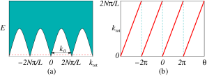
Figure 1: (a) The distribution of the total energies and total momenta for low energy states of 1d weakly interacting boson liquid. (b) The distribution of the total momenta $k_{\text{tot}}$ for low energy many-body states, and its dependence on the $U(1)$ symmetry twist $\theta$.

From the low energy effective field theory, we find that the low energy excitations are labeled by $(N\in\mathbb{N},m\in\mathbb{Z},n_{k}\in\mathbb{N})$. The total energy and total momentum of those excitations are given by (in the presendence a constant $U(1)$ connection $a$ describing the $U(1)$ symmetry twist)

$$E =\frac{N}{2M_{b}}(\frac{2\pi m}{L}+a)^{2}+\frac{g}{2}(N-\bar{N})^{2}+\sum_{k\neq 0}(n_{k}+\frac{1}{2})v|k|,$$

$$k_{\text{tot}} =\int\hskip 1.0pt\mathrm{d}x\,\rho(\partial_{x}+a)\phi=N(\frac{2\pi m}{L}+a)+\sum_{k\neq 0}n_{k}k,$$ (4)

where $N=\bar{N}+\delta N$ is the total number of bosons in the excited state. When $N=\bar{N}$ and $a=0$, the possible values of $(E,k_{\text{tot}})$ are plotted in Fig. 1a.

After quantization, we have the following operator algebra

$$[\phi(x),\delta\rho(y)]=\hskip 1.0pt\mathrm{i}\hskip 1.0pt\delta(x-y),$$ (5)

where $\delta\rho(x)$ is the boson density operator. Since

$$[\delta\rho(y),\hskip 1.0pt\mathrm{e}^{\hskip 1.0pt\mathrm{i}\hskip 1.0pt\phi(x)}]=\delta(x-y)\hskip 1.0pt\mathrm{e}^{\hskip 1.0pt\mathrm{i}\hskip 1.0pt\phi(x)},$$ (6)

$\hskip 1.0pt\mathrm{e}^{\hskip 1.0pt\mathrm{i}\hskip 1.0pt\phi(x)}$ is the boson creation operator.

Let $\varphi(x)=2\pi\int^{x}\hskip 1.0pt\mathrm{d}x^{\prime}\delta\rho(x^{\prime})$. We find that

$$[\varphi(x),\phi(y)] =-2\pi\hskip 1.0pt\mathrm{i}\hskip 1.0pt\Theta(x-y),$$

$$\Theta(x) =\begin{cases}1&\ \ \text{ for }x>0,\\ 0&\ \ \text{ for }x<0,\\ \end{cases}$$ (7)

or

$$\hskip 1.0pt\mathrm{e}^{\hskip 1.0pt\mathrm{i}\hskip 1.0pt\alpha\varphi(x)}\hskip 1.0pt\mathrm{e}^{\hskip 1.0pt\mathrm{i}\hskip 1.0pt\beta\phi(y)} =\hskip 1.0pt\mathrm{e}^{\hskip 1.0pt\mathrm{i}\hskip 1.0pt\beta\phi(y)}\hskip 1.0pt\mathrm{e}^{\hskip 1.0pt\mathrm{i}\hskip 1.0pt\alpha\varphi(x)}\hskip 1.0pt\mathrm{e}^{\alpha\beta[\phi(y),\varphi(x)]}$$

$$=\hskip 1.0pt\mathrm{e}^{\hskip 1.0pt\mathrm{i}\hskip 1.0pt\beta\phi(y)}\hskip 1.0pt\mathrm{e}^{\hskip 1.0pt\mathrm{i}\hskip 1.0pt\alpha\varphi(x)}\hskip 1.0pt\mathrm{e}^{2\pi\hskip 1.0pt\mathrm{i}\hskip 1.0pt\alpha\beta\Theta(x-y)}$$ (8)

which can also be rewritten as

$$\hskip 1.0pt\mathrm{e}^{-\hskip 1.0pt\mathrm{i}\hskip 1.0pt\alpha\varphi(x)}\hskip 1.0pt\mathrm{e}^{-\hskip 1.0pt\mathrm{i}\hskip 1.0pt\beta\phi(y)}\hskip 1.0pt\mathrm{e}^{\hskip 1.0pt\mathrm{i}\hskip 1.0pt\alpha\varphi(x)}\hskip 1.0pt\mathrm{e}^{\hskip 1.0pt\mathrm{i}\hskip 1.0pt\beta\phi(y)} =\hskip 1.0pt\mathrm{e}^{2\pi\hskip 1.0pt\mathrm{i}\hskip 1.0pt\alpha\beta\Theta(x-y)},$$

$$\hskip 1.0pt\mathrm{e}^{-\hskip 1.0pt\mathrm{i}\hskip 1.0pt\beta\phi(y)}\hskip 1.0pt\mathrm{e}^{-\hskip 1.0pt\mathrm{i}\hskip 1.0pt\alpha\varphi(x)}\hskip 1.0pt\mathrm{e}^{\hskip 1.0pt\mathrm{i}\hskip 1.0pt\beta\phi(y)}\hskip 1.0pt\mathrm{e}^{\hskip 1.0pt\mathrm{i}\hskip 1.0pt\alpha\varphi(x)} =\hskip 1.0pt\mathrm{e}^{-2\pi\hskip 1.0pt\mathrm{i}\hskip 1.0pt\alpha\beta\Theta(x-y)}.$$ (9)

The above expression tells us that that the operator $\hskip 1.0pt\mathrm{e}^{\hskip 1.0pt\mathrm{i}\hskip 1.0pt\alpha\varphi(x)}$ cause a $\hskip 1.0pt\mathrm{e}^{-2\pi\hskip 1.0pt\mathrm{i}\hskip 1.0pt\alpha}$ phase shift for the operator $\hskip 1.0pt\mathrm{e}^{\hskip 1.0pt\mathrm{i}\hskip 1.0pt\phi(y)}$ for $y<x$, and keep $\hskip 1.0pt\mathrm{e}^{\hskip 1.0pt\mathrm{i}\hskip 1.0pt\phi(y)}$ unchanged for $y>x$. So the operator $\hskip 1.0pt\mathrm{e}^{\hskip 1.0pt\mathrm{i}\hskip 1.0pt\varphi(x)}$ increases $m$ by 1, i.e. increase the total momentum by $2\pi\bar{\rho}$. Similarly, the operator $\hskip 1.0pt\mathrm{e}^{\hskip 1.0pt\mathrm{i}\hskip 1.0pt\beta\phi(x)}$ cause a $\hskip 1.0pt\mathrm{e}^{2\pi\hskip 1.0pt\mathrm{i}\hskip 1.0pt\beta}$ phase shift for the operator $\hskip 1.0pt\mathrm{e}^{\hskip 1.0pt\mathrm{i}\hskip 1.0pt\varphi(y)}$ for $y<x$, and keep $\hskip 1.0pt\mathrm{e}^{\hskip 1.0pt\mathrm{i}\hskip 1.0pt\varphi(y)}$ unchanged for $y>x$. So the operator $\hskip 1.0pt\mathrm{e}^{\hskip 1.0pt\mathrm{i}\hskip 1.0pt\phi(x)}$ increases $N=\frac{1}{2\pi}\int\hskip 1.0pt\mathrm{d}x\,\partial_{x}\varphi=\int\hskip 1.0pt\mathrm{d}x\,\delta\rho$ by 1.

From the above results, we see that under the $U(1)$ transformation $\theta$

$$\phi(x)\to\phi(x)+\theta,\ \ \ \ \varphi(x)\to\varphi(x).$$ (10)

Under the $\mathbb{R}$ translation transformation $\delta x$

$$\phi(x)\to\phi(x+\delta x),\ \ \ \ \varphi(x)\to\varphi(x+\delta x)+2\pi\bar{\rho}\delta x.$$ (11)

However, at low energies, for smooth fields and small $\delta x$, we have $\phi(x)\approx\phi(x+\delta x)$ and $\varphi(x)\approx\varphi(x+\delta x)$. Thus under the $\mathbb{R}$ transformation $\delta x$

$$\phi(x)\to\phi(x),\ \ \ \ \varphi(x)\to\varphi(x)+2\pi\bar{\rho}\delta x.$$ (12)

This way, the $\mathbb{R}$ symmetry becomes an internal symmetry in the low energy effective field theory (3). We will see that $U(1)\times\mathbb{R}$, when viewed as an internal symmetry, has a mixed anomaly.

We note that $\hskip 1.0pt\mathrm{e}^{\hskip 1.0pt\mathrm{i}\hskip 1.0pt\varphi(x)}$ is a local operator and $\int\hskip 1.0pt\mathrm{d}x\,\delta\rho=\frac{1}{2\pi}\int\hskip 1.0pt\mathrm{d}x\,\partial_{x}\varphi$ is an integer. Both imply that $\varphi$ is also an angular variable $\varphi(x,t)\sim\varphi(x,t)+2\pi$. Using the two angular fields $\phi_{1}=:\phi$ and $\phi_{2}=:\varphi$, the low energy effective theory can be written as

$$L_{\text{ph}}=\int\hskip 1.0pt\mathrm{d}x\;\big{(}\bar{\rho}\partial_{t}\phi_{1}+\frac{K_{IJ}}{4\pi}\partial_{x}\phi_{I}\partial_{t}\phi_{J}-\frac{V_{IJ}}{2}\partial_{x}\phi_{I}\partial_{x}\phi_{J}\big{)}$$ (13)

where

$$K=\begin{pmatrix}0&1\\ 1&0\\ \end{pmatrix}.$$ (14)

and $V$ is a positive definite symmetric matrix.

II.2 The universal properties of the gapless phase

From eqn. (II.1), we see that the total momentum $k_{\text{tot}}$ depends on the $U(1)$ symmetry twist

$$k_{\text{tot}}=\rho\theta,\ \ \ \text{ where }\theta=\int\hskip 1.0pt\mathrm{d}x\;a=aL,\ \ \rho=\frac{N}{L}.$$ (15)

However, since the state is gapless, there are many low energy states with different momenta. So we do not know $k_{\text{tot}}$ to be the momentum of which low energy states. To make our statement meaningful, we consider two low energy states $|\Psi_{N}\rangle$ of $N$ bosons. Let $k_{\text{tot}}$ be the total momenta of $|\Psi_{N}\rangle$. Since there are many different low energy states $|\Psi_{N}\rangle$’s, we have many different values of $k_{\text{tot}}$. In other words, we have a distribution of $k_{\text{tot}}$’s. Such a distribution is plotted in Fig. 1b.

From the distribution pattern in Fig. 1, we see two universal properties: the period in the distribution and the $\theta=aL$ dependence of the distribution

$$k_{0}=2\pi\bar{\rho},\ \ \ \ \ \frac{\hskip 1.0pt\mathrm{d}k_{\text{tot}}}{\hskip 1.0pt\mathrm{d}\theta}=\bar{\rho},$$ (16)

which do not depend on the small changes in the interactions and the dispersion of the bosons, unless those changes cause a phase transition. Thus we say they are universal properties that characterize the gapless phase. The two universal properties are closely related $(2\pi)^{-1}k_{0}=\frac{\hskip 1.0pt\mathrm{d}k_{\text{tot}}}{\hskip 1.0pt\mathrm{d}\theta}=\bar{\rho}$. We call $\bar{\rho}$ an index for the gapless phase. Physically $\bar{\rho}$ is nothing but the density of the $U(1)$ charges in the ground state.

Let us give a argument why $\frac{\hskip 1.0pt\mathrm{d}k_{\text{tot}}}{\hskip 1.0pt\mathrm{d}\theta}$ is universal. Let us assume the $U(1)$ symmetry twist is described by a boundary condition on single-particle wave function at $x_{0}$: $\psi(x_{0}+0^{+})=\hskip 1.0pt\mathrm{e}^{\hskip 1.0pt\mathrm{i}\hskip 1.0pt\theta}\psi(x_{0}-0^{+})$. A usual translation $x\to x+\Delta x$ will shift the symmetry twist from $x_{0}$ to $x_{0}+\Delta x$. So the symmetry twist breaks the translation symmetry. But we can redefine the translation operator to be the usual translation plus a $U(1)$ transformation $\psi(x)\to\hskip 1.0pt\mathrm{e}^{\hskip 1.0pt\mathrm{i}\hskip 1.0pt\theta}\psi(x)$ for $x\in[x_{0},x_{0}+\Delta x]$. The new translation operator generates the translation symmetry in the presence of the $U(1)$ symmetry twist. Due to the $U(1)$ transformation $\psi(x)\to\hskip 1.0pt\mathrm{e}^{\hskip 1.0pt\mathrm{i}\hskip 1.0pt\theta}\psi(x)$ for $x\in[x_{0},x_{0}+\Delta x]$, the eigenvalue of the new translation operator has a $\theta$ dependence given by $(\hskip 1.0pt\mathrm{e}^{\hskip 1.0pt\mathrm{i}\hskip 1.0pt\theta})^{\bar{\rho}\Delta x}$, where $\bar{\rho}\Delta x$ is the total $U(1)$ charges in the interval $[x_{0},x_{0}+\Delta x]$. In other words the total momentum has a $\theta$ dependence given by $\theta\bar{\rho}$. This is the reason why $\frac{\hskip 1.0pt\mathrm{d}k_{\text{tot}}}{\hskip 1.0pt\mathrm{d}\theta}=\bar{\rho}$. Since $\theta=0$ and $\theta=2\pi$ are equivalent, therefore $\frac{\hskip 1.0pt\mathrm{d}k_{\text{tot}}}{\hskip 1.0pt\mathrm{d}\theta}=\bar{\rho}$ implies the periodicy in Fig. 1, with the period $k_{0}=2\pi\bar{\rho}$. The above discussion does not depend on interactions and boson dispersion. So the results (16) are universal properties.

II.3 Mixed anomaly for $U(1)\times\mathbb{R}$ symmetry

From the above argument, we also see that the shift of the low energy momentum distribution by the $U(1)$ symmetry twist, $\frac{\hskip 1.0pt\mathrm{d}k_{\text{tot}}}{\hskip 1.0pt\mathrm{d}\theta}=\bar{\rho}$, is an invariant not only against small perturbations that preserve the $U(1)\times\mathbb{R}$ symmetry, but is also an invariant against large symmetry-preserving perturbations that can drive through a phase transition. The invariant for large perturbations is actually an anomaly.’t Hooft (1980) This is because, under a new point of view,Wen (2013); Kong and Wen (2014) an anomaly corresponds to an SPT or topological order in one higher dimension.Wen (2013); Kong and Wen (2014) Any large perturbations and phase transitions cannot change the SPT or topological order in one higher dimension.

In our case, we can view $\frac{\hskip 1.0pt\mathrm{d}k_{\text{tot}}}{\hskip 1.0pt\mathrm{d}\theta}=\bar{\rho}$ as an anomaly in the low energy effective field theories (3) and (13). We see that the topological term $\bar{\rho}(x,t)\dot{\phi}(x,t)$ in the low energy effective field theory determine the anomaly. In fact, such an anomaly is a mixed anomaly between $U(1)$ symmetry and the translation $\mathbb{R}$ symmetry, which describe how an $U(1)$ symmetry twist can change the total momentum (i.e. $\frac{\hskip 1.0pt\mathrm{d}k_{\text{tot}}}{\hskip 1.0pt\mathrm{d}\theta}\neq 0$).

The presence of the anomaly implies that the ground state of the system must be either gapless or have a non-trivial topological order. Since there is no non-trivial topological order in 1d, the ground state must be gapless. In other words,

the field theories in eqn. (3) and eqn. (13) with $\bar{\rho}\neq 0$ must be gapless regardless the interaction term described by $\cdots$, as long as the $U(1)\times\mathbb{R}$ symmetry is preserved. On the other hand, when $\bar{\rho}=0$, the field theories in eqn. (3) and eqn. (13) allow a gapped phase with $U(1)\times\mathbb{R}$ symmetry.

The mixed anomaly between the $U(1)$ symmetry and the $\mathbb{R}$ symmetry can also be detected via the patch symmetry transformations studied in Ref. Ji and Wen, 2020. The $U(1)$ patch symmetry transformations are given by

$$W_{U(1)}(x,y)=\hskip 1.0pt\mathrm{e}^{\hskip 1.0pt\mathrm{i}\hskip 1.0pt2\pi\alpha\int_{x}^{y}\hskip 1.0pt\mathrm{d}x\rho}=\hskip 1.0pt\mathrm{e}^{\hskip 1.0pt\mathrm{i}\hskip 1.0pt\alpha(\varphi(y)-\varphi(x))}\hskip 1.0pt\mathrm{e}^{\hskip 1.0pt\mathrm{i}\hskip 1.0pt2\pi\alpha\bar{\rho}(y-x)},$$ (17)

which perform the $U(1)$ transformation, $\phi\to\phi+\alpha$, on the segment $[x,y]$. The $\mathbb{R}$ patch symmetry transformations are given by

$$W_{\mathbb{R}}(x,y)=\hskip 1.0pt\mathrm{e}^{\hskip 1.0pt\mathrm{i}\hskip 1.0pt\bar{\rho}\Delta x(\phi(y)-\phi(x))}.$$ (18)

which perform the $\mathbb{R}$ transformation (the translation $\Delta x$) on the segment $[x,y]$. In the low energy limit, $k\to 0$. So for a finite $\Delta x$ the translation is trivial for the phonon modes. The translation $\Delta x$ has a non-trivial actions only on sector labeled by different $N$’s and $m$’s. For a translation $\Delta x$ that acts on a segment $[x,y]$, its effect is to transfer $U(1)$ charge-$\bar{\rho}\Delta x$ from $x$ to $y$. This is why the $\mathbb{R}$ patch symmetry transformations are given by eqn. (18).

In the low energy effective theories (3) and (13), the $U(1)$ transformation is given by $\phi\to\phi+\theta$. The term $\bar{\rho}\dot{\phi}$ implies $\bar{\rho}$ is the background $U(1)$ charge density. Therefore, the patch translation transformation has a form eqn. (18).

Assume $x_{2}>x_{1}$. We have shown that $W_{U(1)}(x_{1},x_{2})$ shifts $\hskip 1.0pt\mathrm{e}^{\hskip 1.0pt\mathrm{i}\hskip 1.0pt\beta\phi(y)}$ by a phase $\hskip 1.0pt\mathrm{e}^{-\hskip 1.0pt\mathrm{i}\hskip 1.0pt2\pi\alpha\beta}$, if $x_{1}<y<x_{2}$. Therefore

$$\ \ \ \ W_{U(1)}(x_{1},x_{2})W_{\mathbb{R}}(y_{1},y_{2})$$

$$=W_{\mathbb{R}}(y_{1},y_{2})W_{U(1)}(x_{1},x_{2})\hskip 1.0pt\mathrm{e}^{\hskip 1.0pt\mathrm{i}\hskip 1.0pt2\pi\alpha\bar{\rho}\Delta x},$$ (19)

for $x_{1}<y_{1}<x_{2}<y_{2}$. The extra phase factor $\hskip 1.0pt\mathrm{e}^{\hskip 1.0pt\mathrm{i}\hskip 1.0pt2\pi\alpha\bar{\rho}\Delta x}$ indicates the appearance of the mixed $U(1)\times\mathbb{R}$ anomaly. Using the terminology of Ref. Ji and Wen, 2020, we say, the $U(1)$ symmetry and the $\mathbb{R}$ symmetry have a “mutual statistics” between them, as a consequence of the mixed anomaly. So, according to Ref. Ji and Wen, 2020, the $U(1)$ symmetry and the $\mathbb{R}$ are not independent, and we may denote the combined symmetry as $U(1)\vee\mathbb{R}$ to stress the mixed anomaly.

We like to remark that $\phi$ and $\varphi$ fields are cannonial conjugate to each other. We see that the symmetries that shift $\phi$ and $\varphi$ have a mixed anomaly, as captured by non-trivial commutation relation between the patch operators for the symmetry transformation. This is a general mechanism of the appearance of anomaly.

III 1d fermion liquid with $U(1)\times\mathbb{R}$ symmetry

III.1 Weakly interacting 1d gapless fermionic systems

1d gapless fermionic systems with $U(1)\times\mathbb{R}$ symmetry and weak repulsive interaction are also in a gapless phase – a Tomonaga-Luttinger liquid for fermions. The low energy effective theory also has a form

$$L_{\text{ph}}=\int\hskip 1.0pt\mathrm{d}x\; \big{(}\bar{\rho}\dot{\phi}(x,t)+\delta\rho(x,t)\dot{\phi}(x,t)$$

$$-\frac{\bar{\rho}}{2M_{f}}|\partial\phi|^{2}+\frac{1}{2g}(\dot{\phi})^{2}+\ \cdots\big{)}.$$ (20)

Considering non-interacting fermions in a system with periodic boundary condition on a ring of size $L$, we find that the low energy excitations are also labeled by $(N\in\mathbb{N},m\in\mathbb{Z},n_{k}\in\mathbb{N})$. However, the total energies and total momenta of those excitations are given by, for $N=$ odd,

$$E=\frac{N}{2M_{f}}(2\pi\frac{m}{L}+a)^{2}+\frac{g}{2}\delta N^{2}+\sum_{k\neq 0}(n_{k}+\frac{1}{2})v|k|,$$

$$k_{\text{tot}}=N(2\pi\frac{m}{L}+a)+\sum_{k\neq 0}n_{k}k,$$ (21)

and for $N=$ even,

$$E=\frac{N}{2M_{f}}(2\pi\frac{m+\frac{1}{2}}{L}+a)^{2}+\frac{g}{2}\delta N^{2}+\sum_{k\neq 0}(n_{k}+\frac{1}{2})v|k|,$$

$$k_{\text{tot}}=N(2\pi\frac{m+\frac{1}{2}}{L}+a)+\sum_{k\neq 0}n_{k}k,$$ (22)

where $N(2\pi\frac{m}{L}+a)$ or $N(2\pi\frac{m+\frac{1}{2}}{L}+a)$ are the momentum of center of mass.

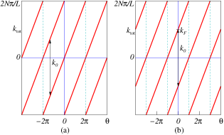
Figure 2: The distribution of the total momenta $\Delta k_{\text{tot}}$ and its dependence on the $U(1)$ symmetry twist, for a weakly interacting 1d fermion liquid.

Again, we consider low energy states $|\Psi_{N}\rangle$ of $N$ fermions. Let $k_{\text{tot}}$ be the total momenta of $|\Psi_{N}\rangle$. Since there are many different low energy states $|\Psi_{N}\rangle$’s, we have a distribution of $k_{\text{tot}}$’s. Such a distribution is plotted in Fig. 2a for $N_{=}$ odd case, and in Fig. 2b for $N=$ even case. We see that $N=$ odd case and $N=$ even case have different distributions for $k_{\text{tot}}$’s.

The shift of the distribution of $k_{\text{tot}}$ by the $U(1)$ symmetry twist (see Fig. 2) can be interpreted as $U(1)$ symmetry twist producing or pumping momentum. This directly measures the mixed $U(1)\times\mathbb{R}$ anomaly.

We also see that a local operator that create a fermion (i.e. change $N$ by 1) must also change $m$ by $\frac{1}{2}$. Those operators have a form $\hskip 1.0pt\mathrm{e}^{\hskip 1.0pt\mathrm{i}\hskip 1.0pt(\phi\pm\frac{1}{2}\varphi)}$, where $\partial_{x}\varphi=2\pi\delta\rho$. Since the allowed operators are generated by $\hskip 1.0pt\mathrm{e}^{\hskip 1.0pt\mathrm{i}\hskip 1.0pt(\phi\pm\frac{1}{2}\varphi)}$, the following fields

$$\phi_{1}=\phi+\frac{1}{2}\varphi,\ \ \ \ \ \phi_{2}=\phi-\frac{1}{2}\varphi$$ (23)

are angular fields: $\phi_{i}\sim\phi_{i}+2\pi$. Using

$$\phi=\frac{1}{2}(\phi_{1}+\phi_{2}),\ \ \ \ \ \varphi=\phi_{1}-\phi_{2},$$ (24)

we find the low energy effective theory to be

$$L =\int\hskip 1.0pt\mathrm{d}x\;\big{(}\frac{\bar{\rho}}{2}\partial_{t}(\phi_{1}+\phi_{2})$$

$$\ \ \ \ \ \ \ \ +\frac{1}{4\pi}\partial_{x}(\phi_{1}-\phi_{2})\partial_{t}(\phi_{1}+\phi_{2})-\frac{V_{IJ}}{2}\partial_{x}\phi_{I}\partial_{x}\phi_{J}\big{)}$$

$$=\int\hskip 1.0pt\mathrm{d}x\;\big{(}\frac{\bar{\rho}}{2}\partial_{t}(\phi_{1}+\phi_{2})+\frac{1}{4\pi}(\partial_{x}\phi_{1}\partial_{t}\phi_{2}-\partial_{x}\phi_{2}\partial_{t}\phi_{1})$$

$$\ \ \ \ \ \ \ \ +\frac{K_{IJ}}{4\pi}\partial_{x}\phi_{I}\partial_{t}\phi_{J}-\frac{V_{IJ}}{2}\partial_{x}\phi_{I}\partial_{x}\phi_{J}\big{)},$$

$$K =\begin{pmatrix}1&0\\ 0&-1\\ \end{pmatrix},\ \ \ \ V=\text{positive definite}.$$ (25)

Here, we have been careful to keep the total derivative terms $\frac{\bar{\rho}}{2}\partial_{t}(\phi_{1}+\phi_{2})+\frac{1}{4\pi}(\partial_{x}\phi_{1}\partial_{t}\phi_{2}-\partial_{x}\phi_{2}\partial_{t}\phi_{1})$. Those are topological terms that do not affect the classical equation of motion, but have effects in quantum theory.

Effective theory similar to the above form has been obtained before for edge state of fractional quantum Hall states.Wen (1992, 1995) But here we have to be more careful in keeping the topological term $\bar{\rho}\partial_{t}\phi_{1}$, which describes the mixed anomaly of $U(1)\times\mathbb{R}$ symmetry for the fermionic system.

We like to mention that the patch symmetry transformations are determined from the low energy effective theories (III.1) or (III.1), and are still given by eqn. (17) and eqn. (18). So the mixed anomaly can still be detected via commutation relation of the patch symmetry transformations (II.3).

In fact, eqn. (III.1) is the low energy effective theory for a fermion system with Fermi momentum $k_{F}=\pi\bar{\rho}$. $\frac{1}{2\pi}\partial_{x}\phi_{1}$ describes the density of right-moving fermions and $\frac{1}{2\pi}\partial_{x}\phi_{2}$ describes the density of left-moving fermions. For example, the low energy effective theory for right-moving fermions is given by

$$L=\int\hskip 1.0pt\mathrm{d}x\;\big{(}\frac{k_{F}}{2\pi}\partial_{t}\phi_{1}+\frac{1}{4\pi}\partial_{x}\phi_{1}\partial_{t}\phi_{1}-\frac{V_{11}}{2}\partial_{x}\phi_{1}\partial_{x}\phi_{1}\big{)},$$

$$=\int\hskip 1.0pt\mathrm{d}x\;\big{(}\bar{\rho}_{1}\partial_{t}\phi_{1}+\frac{1}{4\pi}\partial_{x}\phi_{1}\partial_{t}\phi_{1}-\frac{V_{11}}{2}\partial_{x}\phi_{1}\partial_{x}\phi_{1}\big{)}.$$ (26)

In the above expression, we stress the direction connection between the topological term and the Fermi momentum $k_{F}$, as well as the direction connection between the topological term and the density of the right-moving fermions: $\bar{\rho}_{1}=\frac{k_{F}}{2\pi}=\frac{1}{2}\bar{\rho}$.

We see that the mixed anomaly of $U(1)\times\mathbb{R}$ symmetry is nothing but a non-zero Fermi momentum $k_{F}$. When $k_{F}=0$, i.e. when mixed anomaly vanishes, the fermion system can have a gapped ground state that does not break the $U(1)\times\mathbb{R}$ symmetry. But when $k_{F}\neq 0$, i.e. in the presence of mixed anomaly, the fermion system cannot have a gapped ground state that does not break the $U(1)\times\mathbb{R}$ symmetry. This is a well known result, but restated in terms of mixed anomaly of $U(1)\times\mathbb{R}$ symmetry.

IV Low energy effective theory of $d$-dimensional Fermi liquid and the mixed $U(1)\times\mathbb{R}^{d}$ anomaly

IV.1 Effective theory for the Fermi surface dynamics

In the last section, we discussed the low energy effective theory of 1d Fermi liquid, which contain a proper topological term that reflects the mixed $U(1)\times\mathbb{R}$ anomaly. In this section, we are going to generalize this result to higher dimensions. The generalization is possible since the higher dimensional Fermi liquid can be viewed as a collection of 1d Fermi liquids.

Let us use $\boldsymbol{k}_{F}$ to parametrize the Fermi surface. We introduce $u(\boldsymbol{x},\boldsymbol{k}_{F})$ to describe the shift of the Fermi surface. Thus the total fermion number is given by

$$N=\bar{N}+\int\hskip 1.0pt\mathrm{d}^{d}\boldsymbol{x}\frac{\hskip 1.0pt\mathrm{d}^{d-1}\boldsymbol{k}_{F}}{(2\pi)^{d}}\,u(\boldsymbol{x},\boldsymbol{k}_{F}).$$ (27)

The total energy is

$$E=\bar{E}+\int\hskip 1.0pt\mathrm{d}^{d}\boldsymbol{x}\frac{\hskip 1.0pt\mathrm{d}^{d-1}\boldsymbol{k}_{F}}{(2\pi)^{d}}\,\frac{|\boldsymbol{v}_{F}(\boldsymbol{k}_{F})|}{2}u^{2}(\boldsymbol{x},\boldsymbol{k}_{F}),$$ (28)

where

$$\boldsymbol{v}_{F}=:\partial_{\boldsymbol{k}}H(\boldsymbol{k}),$$ (29)

is the Fermi velocity and $H(\boldsymbol{k})$ is the single fermion energy.

The equation of motion for the field $u(\boldsymbol{x},\boldsymbol{k}_{F})$ is given by

$$(\partial_{t}+\boldsymbol{v}_{F}\cdot\partial_{\boldsymbol{x}})u(\boldsymbol{x},\boldsymbol{k}_{F})=0$$ (30)

Let us introduce a field $\phi(\boldsymbol{x},\boldsymbol{k}_{F})$ via

$$-\boldsymbol{n}_{F}\cdot\partial_{\boldsymbol{x}}\phi(\boldsymbol{x},\boldsymbol{k}_{F})=u(\boldsymbol{x},\boldsymbol{k}_{F}),$$ (31)

where

$$\boldsymbol{n}_{F}=:\frac{\boldsymbol{v}_{F}}{|\boldsymbol{v}_{F}|}.$$ (32)

The equation of motion for $\phi$ becomes

$$(\partial_{t}+\boldsymbol{v}_{F}\cdot\partial_{\boldsymbol{x}})\big{(}\boldsymbol{n}_{F}\cdot\partial_{\boldsymbol{x}}\phi(\boldsymbol{x},\boldsymbol{k}_{F})\big{)}=0$$ (33)

and the total energy becomes

$$E=\bar{E}+\int\hskip 1.0pt\mathrm{d}^{d}\boldsymbol{x}\frac{\hskip 1.0pt\mathrm{d}^{d-1}\boldsymbol{k}_{F}}{(2\pi)^{d}}\,\frac{|\boldsymbol{v}_{F}(\boldsymbol{k}_{F})|}{2}\boldsymbol{n}_{F}\cdot\partial_{\boldsymbol{x}}\phi(\boldsymbol{x},\boldsymbol{k}_{F})]^{2}.$$ (34)

The phase-space Lagrangian that produces the above equation of motion and total energy is given by

$$L_{\text{ph}}=\int\hskip 1.0pt\mathrm{d}^{d}\boldsymbol{x} \frac{\hskip 1.0pt\mathrm{d}^{d-1}\boldsymbol{k}_{F}}{(2\pi)^{d}}\,\Big{(}-\frac{1}{2}\partial_{t}\phi(\boldsymbol{x},\boldsymbol{k}_{F})\boldsymbol{n}_{F}\cdot\partial_{\boldsymbol{x}}\phi(\boldsymbol{x},\boldsymbol{k}_{F})$$

$$-\frac{|\boldsymbol{v}_{F}(\boldsymbol{k}_{F})|}{2}[\boldsymbol{n}_{F}\cdot\partial_{\boldsymbol{x}}\phi(\boldsymbol{x},\boldsymbol{k}_{F})]^{2}\Big{)}$$ (35)

Repeating a calculation similar to 1d chiral Luttinger liquid,Wen (1992, 1995) we find that after quantization, the operator $\phi(\boldsymbol{x},\boldsymbol{k}_{F})$ has the following commutation relation

$$\ \ \ \ [\phi(\boldsymbol{x}^{\prime},\boldsymbol{k}_{F}^{\prime}),\boldsymbol{n}_{F}\cdot\partial_{\boldsymbol{x}}\phi(\boldsymbol{x},\boldsymbol{k}_{F})]$$

$$=-[\phi(\boldsymbol{x}^{\prime},\boldsymbol{k}_{F}^{\prime}),u(\boldsymbol{x},\boldsymbol{k}_{F})]$$

$$=-\hskip 1.0pt\mathrm{i}\hskip 1.0pt(2\pi)^{d}\delta^{d}(\boldsymbol{x}-\boldsymbol{x}^{\prime})\delta^{d-1}(\boldsymbol{k}_{F}-\boldsymbol{k}_{F}^{\prime})$$ (36)

which reproduce the equation of motion

$$\partial_{t}\phi(\boldsymbol{x},\boldsymbol{k}_{F},t)=\hskip 1.0pt\mathrm{i}\hskip 1.0pt[H,\phi(\boldsymbol{x},\boldsymbol{k}_{F},t)]=-\boldsymbol{v}_{F}\cdot\partial_{\boldsymbol{x}}\phi(\boldsymbol{x},\boldsymbol{k}_{F},t),$$

$$H=\int\hskip 1.0pt\mathrm{d}^{d}\boldsymbol{x}\frac{\hskip 1.0pt\mathrm{d}^{d-1}\boldsymbol{k}_{F}}{(2\pi)^{d}}\,\frac{|\boldsymbol{v}_{F}(\boldsymbol{k}_{F})|}{2}[\boldsymbol{n}_{F}\cdot\partial_{\boldsymbol{x}}\phi(\boldsymbol{x},\boldsymbol{k}_{F})]^{2}$$ (37)

We also see that

$$[N,\phi(\boldsymbol{x},\boldsymbol{k}_{F})]=-\hskip 1.0pt\mathrm{i}\hskip 1.0pt,\ \ \ [N,\hskip 1.0pt\mathrm{e}^{\hskip 1.0pt\mathrm{i}\hskip 1.0pt\phi(\boldsymbol{x},\boldsymbol{k}_{F})}]=\hskip 1.0pt\mathrm{e}^{\hskip 1.0pt\mathrm{i}\hskip 1.0pt\phi(\boldsymbol{x},\boldsymbol{k}_{F})}.$$ (38)

Thus $\hskip 1.0pt\mathrm{e}^{\hskip 1.0pt\mathrm{i}\hskip 1.0pt\phi(\boldsymbol{x},\boldsymbol{k}_{F},t)}$ is the operator that increases $N$ by 1, and the $U(1)$ symmetry transformation is given by

$$\hskip 1.0pt\mathrm{e}^{\hskip 1.0pt\mathrm{i}\hskip 1.0pt\theta N}\phi(\boldsymbol{x},\boldsymbol{k}_{F})\hskip 1.0pt\mathrm{e}^{-\hskip 1.0pt\mathrm{i}\hskip 1.0pt\theta N}=\phi(\boldsymbol{x},\boldsymbol{k}_{F})+\theta.$$ (39)

We see that $\phi(\boldsymbol{x},\boldsymbol{k}_{F})$ is an angular field $\phi(\boldsymbol{x},\boldsymbol{k}_{F})\sim\phi(\boldsymbol{x},\boldsymbol{k}_{F})+2\pi$.

However, in eqn. (IV.1) we only have terms that $\phi(\boldsymbol{x},\boldsymbol{k}_{F})$ couples to $\delta N$. In a compete Lagrangian, $\phi(\boldsymbol{x},\boldsymbol{k}_{F})$ must also couple to $\bar{\rho}$ – the density of the $U(1)$ charge in the ground state. The complete phase-space Lagrangian is given by

$$L_{\text{ph}}=\int\hskip 1.0pt\mathrm{d}^{d}\boldsymbol{x} \frac{\hskip 1.0pt\mathrm{d}^{d-1}\boldsymbol{k}_{F}}{(2\pi)^{d}}\,\Big{(}\frac{\bar{\rho}}{A_{F}}\dot{\phi}(\boldsymbol{x},\boldsymbol{k}_{F})$$

$$-\frac{1}{2}\dot{\phi}(\boldsymbol{x},-\boldsymbol{k}_{F})\boldsymbol{n}_{F}\cdot\partial_{\boldsymbol{x}}\phi(\boldsymbol{x},\boldsymbol{k}_{F})$$

$$-\frac{1}{2}\dot{\phi}(\boldsymbol{x},\boldsymbol{k}_{F})\boldsymbol{n}_{F}\cdot\partial_{\boldsymbol{x}}\phi(\boldsymbol{x},\boldsymbol{k}_{F})$$

$$-\frac{|\boldsymbol{v}_{F}(\boldsymbol{k}_{F})|}{2}[\boldsymbol{n}_{F}\cdot\partial_{\boldsymbol{x}}\phi(\boldsymbol{x},\boldsymbol{k}_{F})]^{2}\Big{)}$$ (40)

where

$$A_{F}=:\int\frac{\hskip 1.0pt\mathrm{d}^{d-1}\boldsymbol{k}_{F}}{(2\pi)^{d}}.$$ (41)

and we have assumed a central reflection symmetry $\boldsymbol{k}_{F}\to-\boldsymbol{k}_{F}$, i.e. $\boldsymbol{v}_{F}(\boldsymbol{k}_{F})=-\boldsymbol{v}_{F}(-\boldsymbol{k}_{F})$ and $\boldsymbol{n}_{F}(\boldsymbol{k}_{F})=-\boldsymbol{n}_{F}(-\boldsymbol{k}_{F})$. The two terms, $\frac{\bar{\rho}}{A_{F}}\dot{\phi}(\boldsymbol{x},\boldsymbol{k}_{F})$ and

$$\int\frac{\hskip 1.0pt\mathrm{d}^{d-1}\boldsymbol{k}_{F}}{(2\pi)^{d}}\,\frac{1}{2}\dot{\phi}(\boldsymbol{x},-\boldsymbol{k}_{F})\boldsymbol{n}_{F}(\boldsymbol{k}_{F})\cdot\partial_{\boldsymbol{x}}\phi(\boldsymbol{x},\boldsymbol{k}_{F}),$$ (42)

are total derivative topological terms.

We know that the volume enclosed by the Fermi surface is directly related to the fermion density $\bar{\rho}$.Luttinger and Ward (1960); Oshikawa (2000) Naively, in our effective theory (IV.1), the parameter $\bar{\rho}$ and Fermi surface $\boldsymbol{k}_{F}$ are not related. In the following, we like to show that in fact $\bar{\rho}$ and the Fermi surface $\boldsymbol{k}_{F}$ are related, from within the effective field theory (IV.1).

Consider a field configuration

$$\phi(\boldsymbol{x},\boldsymbol{k}_{F}) =\boldsymbol{a}\cdot\boldsymbol{x}$$

$$\text{or }\ \ \boldsymbol{n}_{F}\cdot\partial_{\boldsymbol{x}}\phi(\boldsymbol{x},\boldsymbol{k}_{F}) =\boldsymbol{a}\cdot\boldsymbol{n}_{F}=u(\boldsymbol{x},\boldsymbol{k}_{F}).$$ (43)

There are two ways to compute the momentum for such a field configuration.

In the first way, the total momentum is computed via the deformation $u(\boldsymbol{x},\boldsymbol{k}_{F})$ of the Fermi surface (assuming the total momentum of the ground state to be zero)

$$\boldsymbol{k}_{\text{tot}} =\int\hskip 1.0pt\mathrm{d}^{d}\boldsymbol{x}\frac{\hskip 1.0pt\mathrm{d}^{d-1}\boldsymbol{k}_{F}}{(2\pi)^{d}}\,\boldsymbol{k}_{F}u(\boldsymbol{x},\boldsymbol{k}_{F})$$

$$=\int\hskip 1.0pt\mathrm{d}^{d}\boldsymbol{x}\frac{\hskip 1.0pt\mathrm{d}^{d-1}\boldsymbol{k}_{F}}{(2\pi)^{d}}\,\boldsymbol{k}_{F}(\boldsymbol{a}\cdot\boldsymbol{n}_{F}).$$ (44)

Note that $\boldsymbol{n}_{F}$ is the normal direction of the Fermi surface. Therefore

$$\boldsymbol{k}_{\text{tot}}=\int\hskip 1.0pt\mathrm{d}^{d}\boldsymbol{x}\frac{\hskip 1.0pt\mathrm{d}^{d-1}\boldsymbol{k}_{F}}{(2\pi)^{d}}\,\boldsymbol{k}_{F}(\boldsymbol{a}\cdot\boldsymbol{n}_{F})$$ (45)

$$=\int\hskip 1.0pt\mathrm{d}^{d}\boldsymbol{x}\int_{\boldsymbol{k}\in\boldsymbol{k}_{F}+\boldsymbol{a}}\frac{\hskip 1.0pt\mathrm{d}^{d}\boldsymbol{k}_{F}}{(2\pi)^{d}}\,\boldsymbol{k}-\int\hskip 1.0pt\mathrm{d}^{d}\boldsymbol{x}\int_{\boldsymbol{k}\in\boldsymbol{k}_{F}}\frac{\hskip 1.0pt\mathrm{d}^{d}\boldsymbol{k}_{F}}{(2\pi)^{d}}\,\boldsymbol{k},$$

where $\int_{\boldsymbol{k}\in\boldsymbol{k}_{F}}\hskip 1.0pt\mathrm{d}^{d}\boldsymbol{k}_{F}$ means integration over $\boldsymbol{k}$ inside the Fermi surface, and $\int_{\boldsymbol{k}\in\boldsymbol{k}_{F}+\boldsymbol{a}}\hskip 1.0pt\mathrm{d}^{d}\boldsymbol{k}_{F}$ means integration over $\boldsymbol{k}$ inside the shifted Fermi surface (shifted by $\boldsymbol{a}$). Let

$$V_{\boldsymbol{k}_{F}}=:\int_{\boldsymbol{k}\in\boldsymbol{k}_{F}}\hskip 1.0pt\mathrm{d}^{d}\boldsymbol{k}_{F}$$ (46)

be the volume enclosed by the Fermi surface, we see that

$$\boldsymbol{k}_{\text{tot}}=V\frac{V_{\boldsymbol{k}_{F}}}{(2\pi)^{d}}\boldsymbol{a}$$ (47)

where $V$ is the volume of the system.

There is a second way to compute the total momentum $\boldsymbol{k}_{\text{tot}}$. We consider a time dependent translation of the above configuration

$$\phi(\boldsymbol{x},\boldsymbol{k}_{F}) =\boldsymbol{a}\cdot(\boldsymbol{x}+\boldsymbol{x}_{0}(t)).$$ (48)

The effective phase-space Lagrangian for $\boldsymbol{x}_{0}(t)$ is given by

$$L_{\text{ph}}=V\bar{\rho}\boldsymbol{a}\cdot\dot{\boldsymbol{x}}_{0}(t).$$ (49)

We see that $V\bar{\rho}\boldsymbol{a}$ is the canonical momentum of the translation $\boldsymbol{x}_{0}$. Thus, the total momentum of the configuration is

$$\boldsymbol{k}_{tot}=V\bar{\rho}\boldsymbol{a}.$$ (50)

Compare eqn. (47) and eqn. (50), we see that the volume included by the Fermi surface and the fermion density is related

$$\frac{V_{\boldsymbol{k}_{F}}}{(2\pi)^{d}}=\bar{\rho}.$$ (51)

This is the Luttinger theorem.

IV.2 The mixed anomaly in $U(1)\times\mathbb{R}^{d}$ symmetry

As we have pointed out that the topological term $\int\hskip 1.0pt\mathrm{d}^{d}\boldsymbol{x}\frac{\hskip 1.0pt\mathrm{d}^{d-1}\boldsymbol{k}_{F}}{(2\pi)^{d}}\,\big{(}\frac{\bar{\rho}}{A_{F}}\partial_{t}\phi(\boldsymbol{x},\boldsymbol{k}_{F})$ represents a mixed anomaly of $U(1)\times\mathbb{R}^{d}$ symmetry. To see this point, we note that $\boldsymbol{a}$ in eqn. (IV.1) can be viewed as the $U(1)$ symmetry twist. The fact that the $U(1)$ symmetry twist can induce the $\mathbb{R}^{d}$ quantum number (i.e. the momentum) reflects the presence of the mixed anomaly of $U(1)\times\mathbb{R}^{d}$ symmetry. Eqn. (51) indicates that the mixed anomaly can constraint the low energy dynamics, in this case determines the volume enclosed by the Fermi surface.

Figure 3: The total momentum distributions for low energy many-body states for a 2d Fermi liquid, with 1-particle excitations (left, red channal), 2-particle 1-hole excitations (left, green channal), 1-particle 1-hole excitations (right, red channal), and 2-particle 2-hole excitations (right, green channal). The horizental axis is $k_{x}$ and the vertical axis is $k_{y}$.

In the above, we discussed how the $U(1)$ symmetry twist shifts the total momentum of a particular low energy many-body state. However, in practice, we cannot pick a particular low energy many-body state, and see how its momentum is shifted by the $U(1)$ symmetry twist. What can be done is to examine all the low energy many-body low energy states, and their total momentum distribution. The shift of the total momentum distribution by the $U(1)$ symmetry twist measure the mixed $U(1)\times\mathbb{R}^{d}$ anomaly. In Fig. 3, we plot the total momentum distributions for low energy many-body states, with 1-particle excitations, 2-particle 1-hole excitations, 1-particle 1-hole excitations, and 2-particle 2-hole excitations.

The mixed anomaly not only appears in Fermi liquid phases of fermions, it also appears in any other phases of fermions. Thus the mixed anomaly constrain the low energy dynamics in any of those phases. In next section, we consider a phase of fermion, where fermions pair-up to form a boson liquid in $d$-dimensional space.

IV.3 Effective theory of a Fermi liquid in most general setting

In section IV.1, we considered Fermi liquid in free space. In this section, we like to include electromagnetic field in real space, as well as “magnetic field” in $\boldsymbol{k}$ space. We like to find the low energy effective theory of Fermi liquid for this more general situation.

First we consider the dynamics of a single particle in a very general setting. The classical state of the particle is described by a point in phase-space parametrized by $\xi^{I}$. The single particle dynamics is described by a single-particle phase-space Lagrangian:

$$L(\dot{\xi}^{I},\xi^{I})=\int\hskip 1.0pt\mathrm{d}t\ \big{[}a_{I}(\xi^{I})\dot{\xi}^{I}-H(\xi^{I})\big{]},$$ (52)

which gives rise to the following single-particle equation of motion

$$b_{IJ}\dot{\xi}^{J} =\frac{\partial H}{\partial\xi^{I}},\ \ \ \ \ \ b_{IJ}=\partial_{\xi^{I}}a_{J}-\partial_{\xi^{J}}a_{I}.$$ (53)

Here $H(\xi^{I})$ is the single-particle energy for the state $\xi^{I}$, and $a_{I}(\xi^{I})$ is a phase-space vector potential that describes the phase “magnetic” field $b_{IJ}(\xi^{I})$. The phase space “magnetic” field includes both the real space magnetic field and $\boldsymbol{k}$-space “magnetic” field.Thouless et al. (1982); Sundaram and Niu (1999); Xiao et al. (2010)

For a particle in a $d$-dimensional free space described by coordinate-momentum pair $(\boldsymbol{x},\boldsymbol{k})=(x^{i},k_{i})$, $i=1,\cdots,d$, the phase-space magnetic field $b_{IJ}(\xi^{I})$ is a constant (i.e. independent of $\xi^{I}$), since $a_{I}(\xi^{I})\dot{\xi}^{I}=\boldsymbol{k}\cdot\dot{\boldsymbol{x}}$ (i.e. $a_{x^{i}}=k_{i},\ a_{k_{i}}=0$). On the other hand, if there is a non-uniform real space and/or $\boldsymbol{k}$-space magnetic fields, phase-space “magnetic” field $b_{IJ}(\xi^{I})$ will not be uniform.

As a example, let us consider a particle in 3-dimensional space. The phase space is 6-dimensional and is parametrized by $(\xi^{I})=(\boldsymbol{x},\boldsymbol{k})$. The phase-space Lagrangian is given by

$$L =[\boldsymbol{k}\cdot\dot{\boldsymbol{x}}+\boldsymbol{A}(\boldsymbol{x})\cdot\dot{\boldsymbol{x}}+\boldsymbol{\widetilde{A}}(\boldsymbol{k})\cdot\dot{\boldsymbol{k}}]-H(\boldsymbol{k})-V(\boldsymbol{x}).$$ (54)

Here $\boldsymbol{A}(\boldsymbol{x})$ is the real space vector potential for electromagnetic field that only depends on $\boldsymbol{x}$. $\boldsymbol{\widetilde{A}}(\boldsymbol{k})$ is the $\boldsymbol{k}$-space vector potential that is assumed to depend only on $\boldsymbol{k}$. Such a $\boldsymbol{k}$-space vector potential can appear for an electron in a crystal with spin orbital couplings. The corresponding equation of motion is given by

$$\dot{k}_{i} =-\frac{\partial V}{\partial x^{i}}+B_{ij}\dot{x}^{j}, \dot{x}^{i} =\frac{\partial H}{\partial k_{i}}-\widetilde{B}^{ij}\dot{k}_{j},$$

$$\text{or }\ \ \dot{\boldsymbol{k}} =-\frac{\partial V}{\partial\boldsymbol{x}}+\dot{\boldsymbol{x}}\times\boldsymbol{B}, \dot{\boldsymbol{x}} =\frac{\partial H}{\partial\boldsymbol{k}}-\dot{\boldsymbol{k}}\times\widetilde{\boldsymbol{B}}.$$ (55)

where

$$B_{ij} =\partial_{x^{i}}A_{j}-\partial_{x^{j}}A_{i}, \widetilde{B}^{ij} =\partial_{k_{i}}\widetilde{A}^{j}-\partial_{k_{j}}\widetilde{A}^{i},$$

$$\text{or }\ \ \boldsymbol{B} =\partial_{\boldsymbol{x}}\times\boldsymbol{A}, \widetilde{\boldsymbol{B}} =\partial_{\boldsymbol{k}}\times\widetilde{\boldsymbol{A}}.$$ (56)

Now consider a many-fermion system which is described by a particle-number distribution $g(\xi^{I})$. The meaning of the distribution $g(\xi^{I})$ is given by

$$\hskip 1.0pt\mathrm{d}N=g(\xi^{I})\text{Pf}[b(\xi^{I})]\frac{\hskip 1.0pt\mathrm{d}^{2d}\xi^{I}}{(2\pi)^{d}},$$ (57)

where $\hskip 1.0pt\mathrm{d}N$ is the number of fermions in the phase-space volume $\hskip 1.0pt\mathrm{d}^{2d}\xi^{I}$, and $\text{Pf}[b(\xi^{I})]$ is the Pfaffian of the $2d\times 2d$ anti-symmetric matrix

$$[b(\xi^{I})]_{IJ}=b_{IJ}(\xi^{I}).$$ (58)

In fact $g(\xi^{I})$ have a meaning as the occupation number per orbital, since the number of orbitals (i.e. the single particle quantum states) in the phase-space volume $\hskip 1.0pt\mathrm{d}^{2d}\xi^{I}$ is given by $\text{Pf}[b(\xi^{I})]\frac{\hskip 1.0pt\mathrm{d}^{2d}\xi^{I}}{(2\pi)^{d}}$.

The above interpretation is correct since under the time evolution (53), the scaled phase-space volume $\text{Pf}[b(\xi^{I})]\frac{\hskip 1.0pt\mathrm{d}^{2d}\xi^{I}}{(2\pi)^{d}}$ is time independent, which corresponds to the unitary time evolution in quantum theory. To show such a result, we first choose a phase space coordinate such that $b_{IJ}$ is uniform in the phase space. In this case, the time evolution $\dot{\xi}^{I}$ is described by a divergent-less vector field, $\frac{\partial H}{\partial\xi^{I}}$, in the phase space, and the phase-space volume $\hskip 1.0pt\mathrm{d}^{2d}\xi^{I}$ is time independent. We note that the phase-space volume given by the combination $\text{Pf}[b(\xi^{I})]\frac{\hskip 1.0pt\mathrm{d}^{2d}\xi^{I}}{(2\pi)^{b}}$ invariant under the coordinate transformation. Such an invariant combination is invariant under the time evolution (53) for a general coordinate, since the equation of motion is covariant under the coordinate transformation. We see that the phase space has a simpletic geometry.

For our example (54), the 6-by-6 matrix $b_{IJ}$ is given by

$$(b_{IJ})=\begin{pmatrix}B_{ij}&\delta_{ij}\\ -\delta_{ij}&\widetilde{B}^{ij}\\ \end{pmatrix}$$ (59)

We find that

$$\text{Pf}(b) =\text{Pf}\begin{pmatrix}B_{ij}&\delta_{ij}\\ -\delta_{ij}&\widetilde{B}^{ij}\\ \end{pmatrix}$$

$$=\text{Pf}(B,\widetilde{B})=1+B_{ij}\widetilde{B}^{ji}+O(B_{ik}\widetilde{B}^{kj})^{2}.$$ (60)

The effective theory for the Fermi liquid in such a general setting is simply a hydrodynamical theory for an incompressible fluild in the phase space. In the following, we will write down such a theory for small fluctuations near the ground state. First, the ground state of the Fermi liquid is described by the following distribution (or phase-space density)

$$\bar{g}(\xi^{I})=\begin{cases}1,&\text{ for }H(\xi^{I})<0,\\ 0,&\text{ for }H(\xi^{I})>0.\\ \end{cases}$$ (61)

The generalized Fermi surface is the $(2d-1)$-dimensional sub-manifold in the phase space where $\bar{g}(\xi^{I})$ has a jump. A many-body collective excitation is described by another incompressible distribution $g(\xi^{I})=0,1$. For low energy collective excitations near the ground state, we may describe such an incompressible distribution via the displacement of the generalized Fermi surface

$$u(\xi^{I}_{F})=\sqrt{\sum_{I}(\Delta\xi^{I})^{2}},$$ (62)

where $\xi^{I}_{F}$ parametrize the $2d-1$-dimensional generalized Fermi surface, and $\Delta\xi^{I}$ describe the shift of the generalized Fermi surface in the normal direction.

Let us introduce an integration over the generalized Fermi surface

$$\int\text{Pf}[b(\xi^{I})]\frac{\hskip 1.0pt\mathrm{d}^{2d-1}\xi_{F}}{(2\pi)^{d}}=:\int\text{Pf}[b(\xi^{I})]\frac{\hskip 1.0pt\mathrm{d}^{2d}\xi}{(2\pi)^{d}}\,|\partial_{\xi^{I}}\bar{g}|$$ (63)

The number of fermions in the collective excited state described by $u(\xi^{I})$ is given by

$$N =\int\text{Pf}(b)\frac{\hskip 1.0pt\mathrm{d}^{2d}\xi}{(2\pi)^{d}}\,g(\xi^{I})$$

$$=\bar{N}+\int\text{Pf}(b)\frac{\hskip 1.0pt\mathrm{d}^{2d-1}\xi_{F}}{(2\pi)^{d}}\,u(\xi^{I}_{F})$$ (64)

The energy of the collective excited state is given by

$$E =\bar{E}+\int\text{Pf}(b)\frac{\hskip 1.0pt\mathrm{d}^{2d-1}\xi_{F}}{(2\pi)^{d}}\,\frac{1}{2}|h_{.}|u^{2}(\xi^{I}_{F})$$ (65)

where

$$h_{I}=:\partial_{\xi^{I}}H,\ \ \ \ \ |h_{.}|=:\sqrt{\sum_{I}h_{I}^{2}}.$$ (66)

The equation of the motion of $u(\xi^{I}_{F},t)$ can be obtained in two ways. First, we note that $|h_{I}|u$ is the single particle energy, which is invariant under the single particle time evolution $\xi^{I}_{F}(t)$ that satisfies the single-particle equation of motion (53). Thus

$$\frac{\hskip 1.0pt\mathrm{d}}{\hskip 1.0pt\mathrm{d}t}|h_{.}|u(\xi^{I}_{F}(t),t)=0,$$ (67)

This allows us to obtain the equation of motion for $u(\xi^{I}_{F},t)$ field using the single-particle equation of motion (53)

$$\Big{(}\partial_{t}+h^{I}(\xi^{I}_{F})\partial_{\xi^{I}}\Big{)}|h_{.}|(\xi^{I}_{F})u(\xi^{I}_{F},t)=0,$$ (68)

where

$$h^{I}=b^{IJ}h_{J}$$ (69)

and the repeated index $J$ is summed. Here $b^{IJ}$ is the matrix inversion of of $b_{IJ}$:

$$b_{IJ}b^{JK}=\delta_{IK}.$$ (70)

Second, we note that $\text{Pf}(b)u$ is the density of fermions on the generalized Fermi surface (see eqn. (IV.3)). The corresponding current density is given by $h^{I}\text{Pf}(b)u$, since $\dot{\xi}^{I}=h^{I}$ (see eqn. (53)). The fermion conservation gives us another equation of motion for $u(\xi^{I}_{F},t)$:

$$\partial_{t}\text{Pf}\big{(}b(\xi^{I}_{F})\big{)}u(\xi^{I}_{F},t)+\partial_{\xi^{I}}\Big{(}h^{I}(\xi^{I}_{F})\text{Pf}\big{(}b(\xi^{I}_{F})\big{)}u(\xi^{I}_{F},t)\Big{)}=0.$$ (71)

Since the single-particle dynamics leads to the two equations, so they they must be consistent. This requires that

$$|h.|(\partial_{t}+\partial_{\xi^{I}}h^{I})\text{Pf}(b)u=\text{Pf}(b)(\partial_{t}+h^{I}\partial_{\xi^{I}})|h.|u.$$ (72)

In other words, $h^{I}$, $|h.|$, and $\text{Pf}(b)$ are related, and they satisfy

$$\frac{|h.|}{\text{Pf}(b)}(\partial_{t}+\partial_{\xi^{I}}h^{I})\frac{\text{Pf}(b)}{|h_{.}|}=\partial_{t}+h^{I}\partial_{\xi^{I}}.$$ (73)

Let us introduce a scalar field $\phi(\xi^{I}_{F},t)$ via

$$-|h_{.}|^{-1}h^{I}\partial_{\xi^{I}_{F}}\phi(\xi^{I}_{F},t)=u(\xi^{I}_{F},t),$$ (74)

The equation of motion for $\phi$ is given by

$$(\partial_{t}+h^{I}\partial_{\xi^{I}})h^{J}\partial_{\xi^{I}_{F}}\phi=0,$$ (75)

which can be simplified further as

$$(\partial_{t}+h^{I}\partial_{\xi^{I}})\phi=0.$$ (76)

since $h^{I}(\xi^{I}_{F})$ does not depend on time.

The above equation of motion and the expression of total energy (65) allow us to determine the phase-space Lagrangian

$$L_{\text{ph}}=-\int\frac{\hskip 1.0pt\mathrm{d}^{2d-1}\xi_{F}}{(2\pi)^{d}}\,\frac{\text{Pf}(b)}{2|h_{.}|}\Big{(}\dot{\phi}h^{I}\partial_{\xi^{I}_{F}}\phi+[h^{I}\partial_{\xi^{I}_{F}}\phi]^{2}\Big{)},$$ (77)

up to total derivative topological terms.

To include topological terms, we assume a symmetry described by a map in phase space

$$\xi^{I}\to\bar{\xi}^{I},\ \ \ \ h^{I}(\xi^{I})=-h^{I}(\bar{\xi}^{I}),$$ (78)

which generalize the $\boldsymbol{k}_{F}\to-\boldsymbol{k}_{F}$ symmetry used before. The phase-space Lagrangian can now be written as

$$L_{\text{ph}} =\int\frac{\hskip 1.0pt\mathrm{d}^{2d-1}\xi_{F}}{(2\pi)^{d}}\,\Big{[}\frac{\bar{N}}{VA_{F}}\dot{\phi}(\xi^{I},t)$$

$$\ \ \ \ \ \ \ -\frac{\text{Pf}\big{(}b(\xi^{I})\big{)}}{2|h_{.}(\xi^{I})|}\Big{(}\dot{\phi}(\bar{\xi}^{I},t)h^{I}(\xi^{I})\partial_{\xi^{I}_{F}}\phi(\xi^{I},t)$$ (79)

$$+ \dot{\phi}(\xi^{I},t)h^{I}(\xi^{I})\partial_{\xi^{I}_{F}}\phi(\xi^{I},t)+\big{[}h^{I}(\xi^{I})\partial_{\xi^{I}_{F}}\phi(\xi^{I},t)\big{]}^{2}\Big{)}\Big{]},$$

where $\bar{N}$ is the number of fermnions in the ground state, and

$$VA_{F}=\int\frac{\hskip 1.0pt\mathrm{d}^{2d-1}\xi_{F}}{(2\pi)^{d}}\,1$$ (80)

is the total volume of generalized Fermi surface.

Fro the first three terms in eqn. (IV.3), we see that $\dot{\phi}(\xi^{I},t)$ directly couples to the total density of fermions

$$N=\int\frac{\hskip 1.0pt\mathrm{d}^{2d-1}\xi_{F}}{(2\pi)^{d}}\,\Big{[}\frac{\bar{N}}{VA_{F}} -\frac{\text{Pf}\big{(}b(\xi^{I})\big{)}}{2|h_{.}(\xi^{I})|}\Big{(}h^{I}(\xi^{I})\partial_{\xi^{I}_{F}}\phi(\xi^{I},t)$$

$$-h^{I}(\xi^{I})\partial_{\bar{\xi}^{I}_{F}}\phi(\bar{\xi}^{I},t)\Big{)}\Big{]}.$$ (81)

In particular, the uniform part of $\dot{\phi}(\xi^{I},t)$ couple to total number of fermions

$$L_{\text{ph}}=N\dot{\phi}_{\text{uniform}}(t)+\cdots.$$ (82)

This indicates that $\phi\sim\phi+2\pi$ is an angular field, and the $U(1)$ transformation is given by

$$\phi(\xi^{I},t)\to\phi(\xi^{I},t)+\theta.$$ (83)

IV.4 Effective theory for a Fermi liquid with real space and $\boldsymbol{k}$-space magnetic fields

Now, let us apply the above formalism to develop the low energy effective theory of Fermi liquid, for 3-dimensional fermions with real space magnetic field $\boldsymbol{A}(\boldsymbol{x})$ and $\boldsymbol{k}$-space “magnetic” field $\widetilde{\boldsymbol{A}}(\boldsymbol{k})$. The dynamics of a single fermion is described by eqn. (54) (with $V=0$). We have

$$(h_{I}) =(0,{\boldsymbol{v}}_{F}),\ \ \ \ \ |h_{.}|=|\boldsymbol{v}_{F}|,\ \ {\boldsymbol{v}}_{F}=:\partial_{\boldsymbol{k}}H,$$

$$(h^{I}) =(\widetilde{\boldsymbol{v}}_{F},\boldsymbol{f}),\ \ \ \ \ \text{Pf}(b)=1-2\boldsymbol{B}\cdot\widetilde{\boldsymbol{B}}+\cdots,$$ (84)

$$\widetilde{\boldsymbol{v}}_{F} ={\boldsymbol{v}}_{F}-({\boldsymbol{v}}_{F}\times\boldsymbol{B})\times\widetilde{\boldsymbol{B}}+\cdots,\ \ \boldsymbol{f}=:{\boldsymbol{v}}_{F}\times\boldsymbol{B}+\cdots.$$

Here $\boldsymbol{f}=\dot{\boldsymbol{k}}$ has a physical meaning as the force acting on each fermion. $\widetilde{\boldsymbol{v}}_{F}=\dot{\boldsymbol{x}}$ has a physical meaning as the velocity of each fermion. When $\widetilde{\boldsymbol{A}}\neq 0$, the velocity of a fermion at the Fermi surface is not given by $\boldsymbol{v}_{F}=\partial_{\boldsymbol{k}}H$. $\widetilde{\boldsymbol{v}}_{F}$ is also called the anomalous velocity.Sundaram and Niu (1999)

Substitute the above into eqn. (IV.3), we obtain

$$L_{\text{ph}}=\int\hskip 1.0pt\mathrm{d}^{d}\boldsymbol{x} \frac{\hskip 1.0pt\mathrm{d}^{d-1}\boldsymbol{k}_{F}}{(2\pi)^{d}}\,\Big{(}\frac{\bar{\rho}}{A_{F}}\dot{\phi}(\boldsymbol{x},\boldsymbol{k}_{F})-\frac{\text{Pf}(b)\dot{\phi}(\boldsymbol{x},-\boldsymbol{k}_{F})}{2|\boldsymbol{v}_{F}|}(\widetilde{\boldsymbol{v}}_{F}\cdot\partial_{\boldsymbol{x}}+\boldsymbol{f}\cdot\partial_{\boldsymbol{k}_{F}})\phi(\boldsymbol{x},\boldsymbol{k}_{F},t)$$ (85)

$$-\frac{\text{Pf}(b)\dot{\phi}(\boldsymbol{x},\boldsymbol{k}_{F})}{2|\boldsymbol{v}_{F}|}(\widetilde{\boldsymbol{v}}_{F}\cdot\partial_{\boldsymbol{x}}+\boldsymbol{f}\cdot\partial_{\boldsymbol{k}_{F}})\phi(\boldsymbol{x},\boldsymbol{k}_{F},t)-\frac{\text{Pf}(b)}{2|\boldsymbol{v}_{F}|}\big{[}(\widetilde{\boldsymbol{v}}_{F}\cdot\partial_{\boldsymbol{x}}+\boldsymbol{f}\cdot\partial_{\boldsymbol{k}_{F}})\phi(\boldsymbol{x},\boldsymbol{k}_{F},t)\big{]}^{2}\Big{)}$$

$$\hskip-43.36243pt-\int\hskip 1.0pt\mathrm{d}^{d}\boldsymbol{x}\frac{\hskip 1.0pt\mathrm{d}^{d-1}\boldsymbol{k}_{F}}{(2\pi)^{d}}\frac{\hskip 1.0pt\mathrm{d}^{d-1}\boldsymbol{k}_{F}^{\prime}}{(2\pi)^{d}}\,\,\frac{\text{Pf}(b)\text{Pf}(b^{\prime})V(\boldsymbol{k}_{F},\boldsymbol{k}_{F}^{\prime})}{2|\boldsymbol{v}_{F}||\boldsymbol{v}_{F}^{\prime}|}\Big{(}(\widetilde{\boldsymbol{v}}_{F}\cdot\partial_{\boldsymbol{x}}+\boldsymbol{f}\cdot\partial_{\boldsymbol{k}_{F}})\phi(\boldsymbol{x},\boldsymbol{k}_{F},t)\Big{)}\Big{(}(\widetilde{\boldsymbol{v}}_{F}^{\prime}\cdot\partial_{\boldsymbol{x}}+\boldsymbol{f}^{\prime}\cdot\partial_{\boldsymbol{k}_{F}})\phi(\boldsymbol{x},\boldsymbol{k}_{F}^{\prime},t)\Big{)}.$$

Up to first order in $\boldsymbol{B}$ and $\widetilde{\boldsymbol{B}}$, the above can be simplified

$$L_{\text{ph}}=\int\hskip 1.0pt\mathrm{d}^{d}\boldsymbol{x} \frac{\hskip 1.0pt\mathrm{d}^{d-1}\boldsymbol{k}_{F}}{(2\pi)^{d}}\,\Big{(}\frac{\bar{\rho}}{A_{F}}\dot{\phi}(\boldsymbol{x},\boldsymbol{k}_{F})-\frac{\dot{\phi}(\boldsymbol{x},-\boldsymbol{k}_{F})}{2|\boldsymbol{v}_{F}|}(\boldsymbol{v}_{F}\cdot\partial_{\boldsymbol{x}}+\boldsymbol{f}\cdot\partial_{\boldsymbol{k}_{F}})\phi(\boldsymbol{x},\boldsymbol{k}_{F},t)$$ (86)

$$-\frac{\dot{\phi}(\boldsymbol{x},\boldsymbol{k}_{F})}{2|\boldsymbol{v}_{F}|}(\boldsymbol{v}_{F}\cdot\partial_{\boldsymbol{x}}+\boldsymbol{f}\cdot\partial_{\boldsymbol{k}_{F}})\phi(\boldsymbol{x},\boldsymbol{k}_{F},t)-\frac{1}{2|\boldsymbol{v}_{F}|}\big{[}(\boldsymbol{v}_{F}\cdot\partial_{\boldsymbol{x}}+\boldsymbol{f}\cdot\partial_{\boldsymbol{k}_{F}})\phi(\boldsymbol{x},\boldsymbol{k}_{F},t)\big{]}^{2}\Big{)}$$

$$\hskip-43.36243pt-\int\hskip 1.0pt\mathrm{d}^{d}\boldsymbol{x}\frac{\hskip 1.0pt\mathrm{d}^{d-1}\boldsymbol{k}_{F}}{(2\pi)^{d}}\frac{\hskip 1.0pt\mathrm{d}^{d-1}\boldsymbol{k}_{F}^{\prime}}{(2\pi)^{d}}\,\,\frac{V(\boldsymbol{k}_{F},\boldsymbol{k}_{F}^{\prime})}{2|\boldsymbol{v}_{F}||\boldsymbol{v}_{F}^{\prime}|}\Big{(}(\boldsymbol{v}_{F}\cdot\partial_{\boldsymbol{x}}+\boldsymbol{f}\cdot\partial_{\boldsymbol{k}_{F}})\phi(\boldsymbol{x},\boldsymbol{k}_{F},t)\Big{)}\Big{(}(\boldsymbol{v}_{F}^{\prime}\cdot\partial_{\boldsymbol{x}}+\boldsymbol{f}^{\prime}\cdot\partial_{\boldsymbol{k}_{F}})\phi(\boldsymbol{x},\boldsymbol{k}_{F}^{\prime},t)\Big{)}.$$

Here, we have assumed a central reflection symmetry $\boldsymbol{k}\to-\boldsymbol{k}$, and the mapping $\xi^{I}\to\bar{\xi}^{I}$ is given by $(\boldsymbol{x},\boldsymbol{k})\to(\boldsymbol{x},-\boldsymbol{k})$. We also included the interaction term for the Fermi surface fluctuations, the $V(\boldsymbol{k}_{F},\boldsymbol{k}_{F}^{\prime})$ term, where $\boldsymbol{v}_{F},\boldsymbol{v}_{F}^{\prime}$ are the Fermi velocities at $\boldsymbol{k}_{F},\boldsymbol{k}_{F}^{\prime}$.

Note that the fermion density at the Fermi surface $\boldsymbol{k}_{F}$ is given by (see eqn. (74))

$$u(\boldsymbol{x},\boldsymbol{k}_{F})=-\frac{\boldsymbol{v}_{F}}{|\boldsymbol{v}_{F}|}\cdot\partial_{\boldsymbol{x}}\phi(\boldsymbol{x},\boldsymbol{k}_{F},t)-\frac{\boldsymbol{f}}{|\boldsymbol{v}_{F}|}\cdot\partial_{\boldsymbol{k}_{F}}\phi(\boldsymbol{x},\boldsymbol{k}_{F},t),$$ (87)

and thus the total fermion number density is given by

$$\rho=\bar{\rho}-\int\frac{\hskip 1.0pt\mathrm{d}^{d-1}\boldsymbol{k}_{F}}{(2\pi)^{d}}\,\Big{(}\frac{\boldsymbol{v}_{F}}{|\boldsymbol{v}_{F}|}\cdot\partial_{\boldsymbol{x}}\phi+\frac{\boldsymbol{f}}{|\boldsymbol{v}_{F}|}\cdot\partial_{\boldsymbol{k}_{F}}\phi\Big{)}.$$ (88)

This expression helps us to understand why the interaction term for the Fermi surface fluctuations has a form given in eqn. (86).

The above expression also allows us to see that $\dot{\phi}(\boldsymbol{x},\boldsymbol{k}_{F})$ couples to the total fermion density (see the first three terms in eqn. (86)). Thus $\phi(\boldsymbol{x},\boldsymbol{k}_{F})\sim\phi(\boldsymbol{x},\boldsymbol{k}_{F})+2\pi$ is an angular field and the $U(1)$ symmetry transformation is given by

$$\phi(\boldsymbol{x},\boldsymbol{k}_{F})\to\phi(\boldsymbol{x},\boldsymbol{k}_{F})+\theta.$$ (89)

Eqn. (73) now becomes (to the first order in $\boldsymbol{B}$ and $\widetilde{\boldsymbol{B}}$)

$$\partial_{\boldsymbol{x}}\cdot\boldsymbol{v}_{F}+\partial_{\boldsymbol{k}_{F}}\cdot\boldsymbol{f}=|\boldsymbol{v}_{F}|^{-1}\big{(}\boldsymbol{v}_{F}\cdot\partial_{\boldsymbol{x}}+\boldsymbol{f}\cdot\partial_{\boldsymbol{k}_{F}}\big{)}|\boldsymbol{v}_{F}|$$ (90)

This will help us to compute the equation of motion for the $\phi$ field. The resulting equation of motion is given by (written in terms of $u(\boldsymbol{x},\boldsymbol{k}_{F},t)$)

$$\big{(}\partial_{t}+\boldsymbol{v}_{F}\cdot\partial_{\boldsymbol{x}}+\boldsymbol{f}\cdot\partial_{\boldsymbol{k}_{F}}\big{)}|\boldsymbol{v}_{F}|u(\boldsymbol{x},\boldsymbol{k}_{F},t)+\big{(}\boldsymbol{v}_{F}\cdot\partial_{\boldsymbol{x}}+\boldsymbol{f}\cdot\partial_{\boldsymbol{k}_{F}}\big{)}\int\frac{\hskip 1.0pt\mathrm{d}^{d-1}\boldsymbol{k}_{F}^{\prime}}{(2\pi)^{d}}\,V(\boldsymbol{k}_{F},\boldsymbol{k}_{F}^{\prime})u(\boldsymbol{x},\boldsymbol{k}_{F}^{\prime},t)=0.$$ (91)

The above is the Boltzmann equation which can be use to compute the transport properties after adding the collision terms. In terms of $\phi(\boldsymbol{x},\boldsymbol{k}_{F},t)$, we have

$$\big{(}\partial_{t}+\boldsymbol{v}_{F}\cdot\partial_{\boldsymbol{x}}+\boldsymbol{f}\cdot\partial_{\boldsymbol{k}_{F}}\big{)}\phi(\boldsymbol{x},\boldsymbol{k}_{F},t)+\int\frac{\hskip 1.0pt\mathrm{d}^{d-1}\boldsymbol{k}_{F}^{\prime}}{(2\pi)^{d}}\,\frac{V(\boldsymbol{k}_{F},\boldsymbol{k}_{F}^{\prime})}{|\boldsymbol{v}_{F}^{\prime}|}\big{(}\boldsymbol{v}_{F}^{\prime}\cdot\partial_{\boldsymbol{x}}\phi(\boldsymbol{x},\boldsymbol{k}_{F}^{\prime},t)+\boldsymbol{f}^{\prime}\cdot\partial_{\boldsymbol{k}_{F}}\phi(\boldsymbol{x},\boldsymbol{k}_{F}^{\prime},t)\big{)}=0.$$ (92)

The above equations of motion are valid only to the first order in $\boldsymbol{B}$ and $\widetilde{\boldsymbol{B}}$. The exact equations of motion, in several different forms, are given by

$$\big{(}\partial_{t}+\partial_{\boldsymbol{x}}\cdot\widetilde{\boldsymbol{v}}_{F}+\partial_{\boldsymbol{k}_{F}}\cdot\boldsymbol{f}\big{)}\text{Pf}(b)u(\boldsymbol{x},\boldsymbol{k}_{F},t)+\text{Pf}(b)\big{(}\frac{\widetilde{\boldsymbol{v}}_{F}}{|\boldsymbol{v}_{F}|}\cdot\partial_{\boldsymbol{x}}+\frac{\boldsymbol{f}}{|\boldsymbol{v}_{F}|}\cdot\partial_{\boldsymbol{k}_{F}}\big{)}\int\frac{\hskip 1.0pt\mathrm{d}^{d-1}\boldsymbol{k}_{F}^{\prime}}{(2\pi)^{d}}\,\text{Pf}(b^{\prime})V(\boldsymbol{k}_{F},\boldsymbol{k}_{F}^{\prime})u(\boldsymbol{x},\boldsymbol{k}_{F}^{\prime},t)=0,$$

$$\big{(}\partial_{t}+\widetilde{\boldsymbol{v}}_{F}\cdot\partial_{\boldsymbol{x}}+\boldsymbol{f}\cdot\partial_{\boldsymbol{k}_{F}}\big{)}|\boldsymbol{v}_{F}|u(\boldsymbol{x},\boldsymbol{k}_{F},t)+\big{(}\widetilde{\boldsymbol{v}}_{F}\cdot\partial_{\boldsymbol{x}}+\boldsymbol{f}\cdot\partial_{\boldsymbol{k}_{F}}\big{)}\int\frac{\hskip 1.0pt\mathrm{d}^{d-1}\boldsymbol{k}_{F}^{\prime}}{(2\pi)^{d}}\,\text{Pf}(b^{\prime})V(\boldsymbol{k}_{F},\boldsymbol{k}_{F}^{\prime})u(\boldsymbol{x},\boldsymbol{k}_{F}^{\prime},t)=0,$$ (93)

$$\big{(}\partial_{t}+\widetilde{\boldsymbol{v}}_{F}\cdot\partial_{\boldsymbol{x}}+\boldsymbol{f}\cdot\partial_{\boldsymbol{k}_{F}}\big{)}\phi(\boldsymbol{x},\boldsymbol{k}_{F},t)+\int\frac{\hskip 1.0pt\mathrm{d}^{d-1}\boldsymbol{k}_{F}^{\prime}}{(2\pi)^{d}}\,\frac{\text{Pf}(b^{\prime})}{|\boldsymbol{v}_{F}^{\prime}|}V(\boldsymbol{k}_{F},\boldsymbol{k}_{F}^{\prime})\big{(}\boldsymbol{v}_{F}^{\prime}\cdot\partial_{\boldsymbol{x}}\phi(\boldsymbol{x},\boldsymbol{k}_{F}^{\prime},t)+\boldsymbol{f}^{\prime}\cdot\partial_{\boldsymbol{k}_{F}}\phi(\boldsymbol{x},\boldsymbol{k}_{F}^{\prime},t)\big{)}=0.$$

IV.5 Emergent $U^{\infty}(1)$ symmetry

From the effective theory (85), we see when there is no real space magnetic field $\boldsymbol{B}=0$, we have $\boldsymbol{f}=0$ and the effective theory has a $U^{\infty}(1)$ symmetry generated by

$$\phi(\boldsymbol{x},\boldsymbol{k}_{F})\to\phi(\boldsymbol{x},\boldsymbol{k}_{F})+\theta(\boldsymbol{k}_{F}),$$ (94)

where $\theta(\boldsymbol{k}_{F})$ can be any function of $\boldsymbol{k}_{F}$. This is the so called emergent $U^{\infty}(1)$ symmetry, which a key character of Fermi liquid.Luther (1979); Haldane (1992); Houghton and Marston (1993); Castro Neto and Fradkin (1994); Else et al. (2020) We also see that the above transformation is no longer a symmetry in the presence of real space magnetic field $\boldsymbol{B}\neq 0$. This may be related to the anomaly in the emergent $U^{\infty}(1)$ symmetry discussed in Ref. Else et al., 2020

V Fermion-pair liquid and the mixed $U(1)\times\mathbb{R}^{d}$ anomaly

In this section, we are going to consider a fermion system in $d$-dimensional continuous space, with $U(1)$ particle-number-conservation symmetry and $\mathbb{R}^{d}$ translation symmetry. We assume the space to have a size $L_{1}\times L_{2}\times\cdots\times L_{d}$, and has a periodic boundary condition. We will compute distribution of the total momentum for many-body low energy excitations $\boldsymbol{k}_{\text{tot}}$, and how such a distribution depends on the $U(1)$ symmetry twist described by a constant vector potential $\boldsymbol{a}$.

Using the results from the Appendix A, we find that the low energy effective theory is described by the following phase-space Lagrangian (see eqn. (A.2))

$$L=\int\hskip 1.0pt\mathrm{d}^{d}\boldsymbol{x}\; \big{(}\bar{\rho}_{p}\dot{\phi}_{p}(\boldsymbol{x},t)+\delta\rho_{p}(\boldsymbol{x},t)\dot{\phi}_{p}(\boldsymbol{x},t)$$

$$\ -\frac{\bar{\rho}}{2M_{p}}|\boldsymbol{\partial}\phi_{p}|^{2}-\frac{g}{2}\delta\rho_{p}^{2}+\ \cdots\big{)},$$ (95)

where $\bar{\rho}_{p}=\frac{1}{2}\bar{\rho}$ is the fermion-pair density in the ground state, and $\phi_{p}\sim\phi_{p}+2\pi$ is the angular field for the fermion-pair. The total energy and total crystal momentum of those excitations are given by

$$E =\frac{\bar{N}_{p}}{2M_{p}}\sum_{\mu}(\frac{m_{\mu}}{L_{\mu}}+2a_{\mu})^{2}+\sum_{\boldsymbol{k}\neq 0}(n_{\boldsymbol{k}}+\frac{1}{2})v|\boldsymbol{k}|,$$

$$\boldsymbol{k}_{\text{tot}} =N_{p}\sum_{\mu}(\frac{m_{\mu}}{L_{\mu}}+2a_{\mu})\hat{\boldsymbol{x}}_{\mu}+\sum_{\boldsymbol{k}\neq 0}n_{\boldsymbol{k}}\boldsymbol{k},$$ (96)

We see that the $U(1)$ symmetry twist $\boldsymbol{a}$ induces a change in the total momentum

$$\boldsymbol{k}_{\text{tot}}=2N_{p}\boldsymbol{a}=2\bar{\rho}_{p}\boldsymbol{a}V=\bar{\rho}\boldsymbol{a}V.$$ (97)

Such momentum dependence of the $U(1)$ symmetry twist $\boldsymbol{a}$ reflects the mixed $U(1)\times\mathbb{R}^{d}$ anomaly. Eqn. (97) and eqn. (50) are identical, implies the identical mixed anomaly, which is captured by the topological term $\int\hskip 1.0pt\mathrm{d}^{d}\boldsymbol{x}\,\big{(}\bar{\rho}_{p}\dot{\phi}_{p}(\boldsymbol{x},t)$.

The mixed anomaly can also be measured by the periodicy $k_{0\mu}$ in the distribution of $\boldsymbol{k}_{\text{tot}}$, and the periodicy $\Delta N=2$ in the distribution of $N$, for the low energy excitations. The period in $\mu$-direction times $\Delta N$ is

$$\Delta Nk_{0\mu}=2\frac{N_{p}}{L_{\mu}}=\frac{N}{L_{\mu}}.$$ (98)

The periodices $k_{0\mu}$ and $\Delta N$ are universal low energy properties of the fermion-pair gapless phase. Their product $\Delta Nk_{0\mu}$ is even more robust, since it is invariant even across any phase transitions, and thus correspond to an anomaly.

For the gapless state formed by four-fermion bound states, the periodicies will be

$$k_{0\mu}=\frac{1}{4}\frac{N}{L_{\mu}},\ \ \ \ \ \ \ \ \Delta N=4.$$ (99)

Their product is still $\Delta Nk_{0\mu}=\frac{N}{L_{\mu}}$.

I would like to thank Maissam Barkeshli, Dominic Else, and Senthil Todadri for discussions and comments. This research is partially supported by NSF DMR-2022428 and by the Simons Collaboration on Ultra-Quantum Matter, which is a grant from the Simons Foundation (651440).

Appendix A Dynamical variational approach and low energy effective theory

A.1 Coherent state approach

A quantum state is described by a complex vector

$$|\psi\rangle=\begin{pmatrix}\psi_{1}\\ \psi_{2}\\ \vdots\\ \end{pmatrix}$$

in a Hilbert state, with inner product

$$\langle\phi|\psi\rangle=\sum_{n}\phi^{*}_{n}\psi_{n}.$$ (100)

The motion of a quantum state is described by time dependent vector: $|\psi(t)\rangle$, which satisfy an equation of motion (called Shrödinger equation) with only first order time derivative:

$$\hskip 1.0pt\mathrm{i}\hskip 1.0pt\frac{\hskip 1.0pt\mathrm{d}}{\hskip 1.0pt\mathrm{d}t}|\psi(t)\rangle=\hat{H}|\psi(t)\rangle,$$ (101)

where the hermitian operator $\hat{H}$ is the Hamiltonian.

The Shrödinger equation (101) also has a phase-space Lagrangian description. If we choose the Lagrangian $L$ to be

$$L(\frac{\hskip 1.0pt\mathrm{d}}{\hskip 1.0pt\mathrm{d}t}|\psi\rangle,|\psi\rangle) =\langle\psi(t)|\hskip 1.0pt\mathrm{i}\hskip 1.0pt\frac{\hskip 1.0pt\mathrm{d}}{\hskip 1.0pt\mathrm{d}t}-\hat{H}|\psi(t)\rangle$$

$$=\hskip 1.0pt\mathrm{i}\hskip 1.0pt\psi_{n}^{*}(t)\dot{\psi}_{n}(t)-\psi_{m}^{*}(t)H_{mn}\psi_{n}(t),$$ (102)

then the action $S=\int\hskip 1.0pt\mathrm{d}t\,L(\frac{\hskip 1.0pt\mathrm{d}}{\hskip 1.0pt\mathrm{d}t}|\psi\rangle,|\psi\rangle)$ will be a functional for the paths $|\psi(t)\rangle$ in the Hilbert space. The stationary paths $|\psi_{\text{sta}}(t)\rangle$ of the action will correspond to the solutions of the Shrödinger equation. Since the Shrödinger equation can be derived from the Lagrangian, we can say that the Lagrangian $L(\frac{\hskip 1.0pt\mathrm{d}}{\hskip 1.0pt\mathrm{d}t}|\psi\rangle,|\psi\rangle)$ provides a complete description of a quantum system.

In the variational approach to the ground state, we consider a variational state $|\psi_{\xi^{i}}\rangle$ that depends on variational parameters $\xi^{i}$. We then found an approximation of the ground state $|\psi_{\bar{\xi}^{i}}\rangle$ by choosing $\bar{\xi}^{i}$ that minimize the average energy

$$\bar{H}(\xi^{i})=\langle\psi_{\xi^{i}}|\hat{H}|\psi_{\xi^{i}}\rangle.$$ (103)

If we choose the variational parameters $\xi^{i}$ properly, the low energy excitations are also described by the fluctuations of variational parameters. In other words, the dynamics of the variational parameters $\xi^{i}$ described the low energy excitations. This leads to a dynamical variational approach (or coherent state approach) that gives us a description of both ground state and low energy excitations.

The dynamics of the full quantum system is described by phase-space Lagrangian $L=\langle\psi|\hskip 1.0pt\mathrm{i}\hskip 1.0pt\frac{\hskip 1.0pt\mathrm{d}}{\hskip 1.0pt\mathrm{d}t}-\hat{H}|\psi\rangle$. The dynamics of the variational parameters is described by the evolution of the quantum states in a submanifold of the total Hilbert space, given by the variational states $|\psi_{\xi^{i}}\rangle$. Here we want to obtain the dynamics of the quantum states, restricted to the submanifold parametrized by $\xi^{i}$. Such a dynamics is described by the same phase-space Lagrangian restricted in the submanifold:

$$L(\dot{\xi}^{i},\xi^{i})=\langle\psi_{\xi^{i}(t)}|\hskip 1.0pt\mathrm{i}\hskip 1.0pt\frac{\hskip 1.0pt\mathrm{d}}{\hskip 1.0pt\mathrm{d}t}-\hat{H}|\psi_{\xi^{i}(t)}\rangle=a_{i}(\xi^{i})\dot{\xi}^{i}-\bar{H}(\xi^{i})$$ (104)

where

$$a_{i}=\hskip 1.0pt\mathrm{i}\hskip 1.0pt\langle\psi_{\xi^{i}}|\frac{\partial}{\partial\xi^{i}}|\psi_{\xi^{i}}\rangle,\ \ \ \ \ \ \bar{H}(\xi^{i})=\langle\psi_{\xi^{i}}|\hat{H}|\psi_{\xi^{i}}\rangle$$ (105)

The resulting equation of motion is given by

$$b_{ij}\dot{\xi}^{j}=\frac{\partial\bar{H}}{\partial\xi^{i}},\ \ \ \ \ \ \ b_{ij}=\partial_{i}a_{j}-\partial_{j}a_{i}$$ (106)

which describes the classical motion of $\xi^{i}$.

The above phase-space Lagrangian actually only described the classical dynamics of the variables $\xi^{i}$. The obtain the low energy effective theory for the quantum dynamics of the variables $\xi^{i}$, we need quantize the phase-space Lagrangian (104) to obtain the low energy effective Hilbart space ${\cal H}_{\text{eff}}$ and the low energy effective Hamiltonian $H_{\text{eff}}$ acting with ${\cal H}_{\text{eff}}$. Roughly, the low energy effective Hilbart space ${\cal H}_{\text{eff}}$ is an representation of the operators algebra

$$\hskip 1.0pt\mathrm{i}\hskip 1.0pt[\hat{\xi}^{i},\hat{\xi}^{j}]=b^{ij}(\hat{\xi}^{i}),$$ (107)

where $b^{ij}$ is the inverse of $b_{ij}$: $b_{ij}b^{jk}=\delta_{ik}$. The low energy effective Hamiltonian is given by

$$H_{\text{eff}}=\bar{H}(\hat{\xi}^{i}).$$ (108)

Let us use the above approach to describe hardcore boson on a single site. The total Hilbert space is 2-dimensional, spanned by $|0\rangle$ (no boson) and $|1\rangle$ (one boson). The coherent state is described by a unit vector $\boldsymbol{n}=(n_{x},n_{y},n_{z})\in S^{2}$. We may also use $\theta,\phi$ to describe $\boldsymbol{n}$:

$$n_{x}(\theta,\phi) =\cos\phi\sin\theta,$$

$$n_{x}(\theta,\phi) =\sin\phi\sin\theta,$$

$$n_{z}(\theta,\phi) =\cos\theta.$$ (109)

We can choose the coherent state to be

$$|\boldsymbol{n}(\theta,\phi)\rangle=\begin{pmatrix}\cos\frac{\theta}{2}\\ \hskip 1.0pt\mathrm{e}^{-\hskip 1.0pt\mathrm{i}\hskip 1.0pt\phi}\sin\frac{\theta}{2}\\ \end{pmatrix}$$ (110)

The phase-space Lagrangian to describe the classical dynamics of $\theta,\phi$ is given by

$$L =\sin^{2}\frac{\theta}{2}\dot{\phi}-\bar{H}(\theta,\phi)$$

$$=\rho\dot{\phi}-\bar{H}(\rho,\phi),\ \ \ \ \ \rho\equiv\frac{1-n_{z}}{2}=\sin^{2}\frac{\theta}{2}$$ (111)

We will use $(\rho,\phi)$ to parametrize the phase space, where $\rho\in[0,1]$ has a physical meaning being the average number of bosons on the site. Here we stress that $(\rho,\phi)$ parametrize $S^{2}$. Quantizing the above classical phase-space Lagrangian, we suppose to obtain a quantum system with Hilbert space ${\cal H}=\text{span}(|0\rangle,|1\rangle)$.

A.2 Low energy effective theory of bosonic superfluid phase

Using the above result, we obtain the following low energy effective theory for interacting bosons in a $d$-dimensional cubic lattice with periodic boundary condition, whose sites are labeled by $\boldsymbol{i}$:

$$L=\sum_{\boldsymbol{i}}\rho_{\boldsymbol{i}}\dot{\phi}_{\boldsymbol{i}}-\bar{H}(\rho_{\boldsymbol{i}},\phi_{\boldsymbol{i}}),$$ (112)

where $\phi_{\boldsymbol{i}}\sim\phi_{\boldsymbol{i}}+2\pi$ is an angular variable. If we assume $\rho_{\boldsymbol{i}},\phi_{\boldsymbol{i}}$ to have a smooth dependence on the space coordinate $\boldsymbol{x}\sim\boldsymbol{i}$, the above can be rewritten as a field theory

$$L=\int\hskip 1.0pt\mathrm{d}^{d}\boldsymbol{x}\; \big{(}\bar{\rho}\dot{\phi}(\boldsymbol{x},t)+\delta\rho(\boldsymbol{x},t)\dot{\phi}(\boldsymbol{x},t)$$

$$\ -\frac{\bar{\rho}}{2m}|\boldsymbol{\partial}\phi|^{2}-\frac{g}{2}\delta\rho^{2}+\ \cdots\big{)},$$ (113)

where we have assumed that $\bar{H}(\rho,\phi)$ is minimized as $\rho=\bar{\rho}$ which correspond to average number of bosons per site.

To quantize the above low-energy-effective theory, we expand

$$\delta\rho =\rho_{0}+\sum_{\boldsymbol{k}\neq 0}\rho_{\boldsymbol{k}}\frac{\hskip 1.0pt\mathrm{e}^{\hskip 1.0pt\mathrm{i}\hskip 1.0pt\boldsymbol{k}\cdot\boldsymbol{x}}}{L^{d/2}}$$

$$\phi =\phi_{0}+2\pi\frac{\boldsymbol{m}\cdot\boldsymbol{x}}{L}+\sum_{\boldsymbol{k}\neq 0}\phi_{\boldsymbol{k}}\frac{\hskip 1.0pt\mathrm{e}^{\hskip 1.0pt\mathrm{i}\hskip 1.0pt\boldsymbol{k}\cdot\boldsymbol{x}}}{L^{d/2}},$$ (114)

where $L$ is the size of the cubic lattice. The $\boldsymbol{k}\neq 0$ modes give rise to a collection of quantum oscillators after quantization. $\rho_{0},\phi_{0},\boldsymbol{m}$ describe the $\boldsymbol{k}=0$ mode, where the integer vector $\boldsymbol{m}=(m_{1},\cdots,m_{d})$ describes the winding numbers of the phase $\phi$. The effective Lagrangian for the $\boldsymbol{k}=0$ modes is given by

$$L_{0}=\big{(}L^{d}\bar{\rho}\dot{\phi}_{0}+L^{d}\rho_{0}\dot{\phi}_{0}-\frac{\bar{\rho}L^{d-2}}{2m}(2\pi)^{2}\boldsymbol{m}^{2}-L^{d}\frac{g}{2}\rho_{0}^{2}\big{)}.$$ (115)

After quantization, the $\boldsymbol{k}=0$ mode describes a particle on a ring with $L^{d}\bar{\rho}$ flux through the ring. Let $\hat{L}_{z}\sim L^{d}(\bar{\rho}+\rho_{0})$ be the angular operator of the quantized particle. After quantization, the Hamiltonian is given by

$$\hat{H}_{0}=\frac{\bar{\rho}L^{d-2}}{2m}(2\pi)^{2}\boldsymbol{m}^{2}+\frac{g}{2L^{d}}(\hat{L}_{z}-L^{d}\bar{\rho})^{2}$$ (116)

The many-body low energy excitations are labeled by $(\boldsymbol{m},N,n_{\boldsymbol{k}\neq 0})$, where integer $N$ is the eigenvalues of $\hat{L}_{z}$ (the total number of bosons) and integer $n_{\boldsymbol{k}\neq 0})$ is the number of excited phonons for $\boldsymbol{k}$ mode. The total energy and the total crystal momentum are given by

$$E=\bar{N}\frac{(2\pi)^{2}\boldsymbol{m}^{2}/L^{2}}{2m}+\frac{g}{2}\frac{(N-\bar{N})^{2}}{L^{d}}+\sum_{\boldsymbol{k}\neq 0}(n_{\boldsymbol{k}}+\frac{1}{2})v|\boldsymbol{k}|^{2},$$

$$\boldsymbol{k}_{\text{tot}}=\int\hskip 1.0pt\mathrm{d}^{d}\boldsymbol{x}\;(\bar{\rho}+\delta\rho)\boldsymbol{\partial}\phi=N\frac{2\pi\boldsymbol{m}}{L}+\sum_{\boldsymbol{k}\neq 0}n_{\boldsymbol{k}}\boldsymbol{k}$$ (117)

where the phonon velocity $v=\sqrt{\frac{g\bar{\rho}}{m}}$, and $\bar{N}\equiv L^{d}\bar{\rho}_{0}$.

The above results are very standard, except that we carefully keep the topological term $\bar{\rho}(\boldsymbol{x},t)\dot{\phi}(\boldsymbol{x},t)$ in the Lagrangian. Our quantum system has $U(1)$ particle number conservation symmetry and $\mathbb{Z}^{d}$ lattice translation symmetry. In the continuum field theory (A.2), we take the limit of zero lattice spacing. In this case, both the $U(1)$ and $\mathbb{Z}^{d}$ symmetries are internal symmetries of the field theory. It turns out that the $U(1)\times\mathbb{Z}^{d}$ symmetry has a mixed ’t Hooft anomaly when $\bar{\rho}$ is not an integer, which constrains the low energy dynamics of the interacting bosons.

References

- Kim et al. (1995) Y. B. Kim, P. A. Lee, and X.-G. Wen, Phys. Rev. B 52, 17275 (1995), arXiv:cond-mat/9504063 .
- Luther (1979) A. Luther, Phys. Rev. B 19, 320 (1979).
- Haldane (1992) F. D. M. Haldane, Helv. Phys. Acta. 65, 152 (1992), arXiv:cond-mat/0505529 .
- Houghton and Marston (1993) A. Houghton and J. B. Marston, Phys. Rev. B 48, 7790 (1993).
- Castro Neto and Fradkin (1994) A. H. Castro Neto and E. Fradkin, Phys. Rev. Lett. 72, 1393 (1994).
- Luttinger and Ward (1960) J. M. Luttinger and J. C. Ward, Phys. Rev. 118, 1417 (1960).
- Oshikawa (2000) M. Oshikawa, Phys. Rev. Lett. 84, 3370 (2000), arXiv:cond-mat/0002392 .
- Lieb et al. (1961) E. H. Lieb, T. D. Schultz, and D. C. Mattis, Ann. Phys. (N.Y) 16, 407 (1961).
- Hastings (2004) M. B. Hastings, Phys. Rev. B 69, 104431 (2004), arXiv:cond-mat/0305505 .
- Furuya and Oshikawa (2017) S. C. Furuya and M. Oshikawa, Phys. Rev. Lett. 118, 021601 (2017), arXiv:1503.07292 .
- Cheng et al. (2016) M. Cheng, M. Zaletel, M. Barkeshli, A. Vishwanath, and P. Bonderson, Physical Review X 6, 041068 (2016), arXiv:1511.02263 .
- Po et al. (2017) H. C. Po, H. Watanabe, C.-M. Jian, and M. P. Zaletel, Phys. Rev. Lett. 119, 127202 (2017), arXiv:1703.06882 .
- Lu et al. (2020) Y.-M. Lu, Y. Ran, and M. Oshikawa, Annals of Physics 413, 168060 (2020), arXiv:1705.09298 .
- Lu (2017) Y.-M. Lu, (2017), arXiv:1705.04691 .
- Cheng (2019) M. Cheng, Phys. Rev. B 99, 075143 (2019), arXiv:1804.10122 .
- Jiang et al. (2019) S. Jiang, M. Cheng, Y. Qi, and Y.-M. Lu, (2019), arXiv:1907.08596 .
- Chen et al. (2011) X. Chen, Z.-C. Gu, and X.-G. Wen, Phys. Rev. B 83, 035107 (2011), arXiv:1008.3745 .
- Else et al. (2020) D. V. Else, R. Thorngren, and T. Senthil, , arXiv:2007.07896 (2020), arXiv:2007.07896 .
- Thouless et al. (1982) D. J. Thouless, M. Kohmoto, M. P. Nightingale, and M. den Nijs, Phys. Rev. Lett. 49, 405 (1982).
- Sundaram and Niu (1999) G. Sundaram and Q. Niu, Phys. Rev. 59, 14915 (1999), arXiv:cond-mat/9908003 .
- Xiao et al. (2010) D. Xiao, M.-C. Chang, and Q. Niu, Rev. Mod. Phys. 82, 1959 (2010), arXiv:0907.2021 .
- ’t Hooft (1980) G. ’t Hooft, in Recent Developments in Gauge Theories. NATO Advanced Study Institutes Series (Series B. Physics), Vol. 59, edited by G. ’t Hooft et al. (Springer, Boston, MA., 1980) pp. 135–157.
- Wen (2013) X.-G. Wen, Phys. Rev. D 88, 045013 (2013), arXiv:1303.1803 .
- Kong and Wen (2014) L. Kong and X.-G. Wen, (2014), arXiv:1405.5858 .
- Ji and Wen (2020) W. Ji and X.-G. Wen, Phys. Rev. Research 2, 033417 (2020), arXiv:1912.13492 .
- Wen (1992) X.-G. Wen, Int. J. Mod. Phys. B 6, 1711 (1992).
- Wen (1995) X.-G. Wen, Adv. Phys. 44, 405 (1995), arXiv:cond-mat/9506066 .