Soft Genetic Programming Binary Classifiers

Abstract

The study of the classifier’s design and it’s usage is one of the most important machine learning areas. With the development of automatic machine learning methods, various approaches are used to build a robust classifier model. Due to some difficult implementation and customization complexity, genetic programming (GP) methods are not often used to construct classifiers. GP classifiers have several limitations and disadvantages. However, the concept of "soft" genetic programming (SGP) has been developed, which allows the logical operator tree to be more flexible and find dependencies in datasets, which gives promising results in most cases. This article discusses a method for constructing binary classifiers using the SGP technique. The test results are presented. Source code - https://github.com/survexman/sgp_classifier

1 Introduction

Genetic Programming (GP) is a promising machine learning technique based on the principles of Darwinian evolution to automatically evolve computer programs to solve problems. GP is especially suitable for building a classifier of tree representation. GP is a soft computing search technique, which is used to evolve a tree-structured program toward minimizing the fitness value of it. The distinctive features of GP make it very convenient for classification, and the benefit of it is the flexibility, which allows the algorithm to be adapted to the needs of each particular problem.

A special case of GP studies the logical tree’s development as a solution to a classification problem [1]. Logical trees are composed of boolean, comparison, and arithmetic operators, and they output a boolean value ( true or false). A solution presented as a logical tree is a very convenient way to analyze a dataset and interpret a solution. Figure 1 shows an example of logical tree.

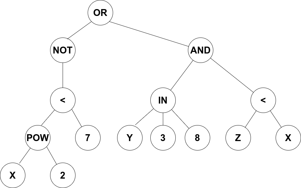
Figure 1: Logical tree example

This logical tree can be rewritten as the following system of inequalities:

$$x^{2}\geq 7\;\lor\;\systeme{y\geq 3,y\leq 8,z<x}$$

Evolving logical trees using GP has the benefit of being able to handle both numerical and categorical data fairly simply. Significant advantage of evolving logical trees is the fact that the trees are highly interpretable to a researcher [4]. Logical trees are portable and can be easily implemented by various tools and programming languages. Another significant advantage is an ability of feature extraction [6].

However, one of the most critical problems in logical trees is a crucial logic change when a tree operator changes [9][11]. Such operator changes occur as a result of crossover and mutation operations [2].

Figure 2: Operator change in Logical Tree

Figure 2 shows a simple change of addition operator to power operator in logical tree:

$$[x>3\;\oplus\;sin(x(y+15)))>0.5]\;\;\mathrel{\vbox{\offinterlineskip\halign{\hfil#\hfil\cr\scalebox{1.2}{.}\cr$\longrightarrow$\cr} }}\;\;[x>3\;\oplus\;sin(xy^{15})))>0.5]$$

And below at Figure 3 we can see the effect of such modification:

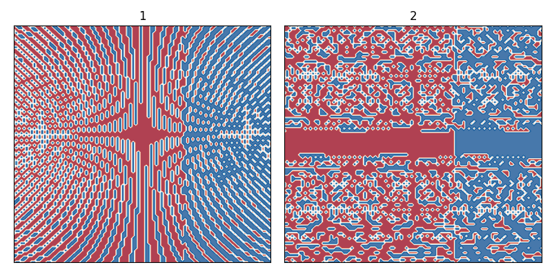
Figure 3: Operator change effect

We see that switching the operator +(y,15) to pow(y,15) changes the logic of the classifier drastically. The more complex the logical tree is, the more this feature is noticeable. This sensitivity of logical trees to tiny changes makes it very difficult to find the appropriate logical tree in a smooth way.

2 Study Roadmap

SGP classifier design is based on classical GP classifier design. First, we will define the architecture of GP classifier. Next, we will introduce the Soft Genetic Programming approach, its design, and evolution operations. Soft Genetic Programming’s main goal is to smoothen evolution improvement and increase the probability of reaching local maxima. After, we will compare the behavior of classical GP Classifier and SGP Classifier. And finally, we will present empirical evidence of the applicability of SGP approach.

3 Genetic Programming Classifier Design

Genetic programming (GP) is a flexible and powerful evolutionary technique with some special features that are suitable for building a classifier of tree representation. [2].

3.1 Operators

We will use the following operators for genetic programming trees [3]:

Boolean:

$$\textrm{OR}:\ \{{0,1}\}^{2}\rightarrow\{{0,1}\}$$

$$\textrm{AND}:\ \{{0,1}\}^{2}\rightarrow\{{0,1}\}$$

$$\textrm{NOT}:\ \{{0,1}\}\rightarrow\{{0,1}\}$$

Comparison:

$$\textrm{>}:\ \mathbb{R}^{2}\rightarrow\{{0,1}\}$$

$$\textrm{<}:\ \mathbb{R}^{2}\rightarrow\{{0,1}\}$$

Mathematical:

$$\textrm{+}:\ \mathbb{R}^{2}\rightarrow\mathbb{R}$$

$$\times:\ \mathbb{R}^{2}\rightarrow\mathbb{R}$$

$$-:\ \mathbb{R}\rightarrow\mathbb{R}$$

Terms:

$$Symbolic:\ \rightarrow X_{i}\;\;\;i\in 1,n,\;where\;n\;-\;number\;of\;features$$

$$Constant:\ \rightarrow\mathbb{R}$$

3.2 Random Tree Generation

Random tree generation is limited by maximum and minimum operator type subchain [8]:

	min	max
Boolean	1	3
Comparison	1	1
Mathematical	1	4
Terms	1	1

3.3 Fitness Function

For fitness function we use Balanced Accuracy:

$$Balanced\;Accuracy=\frac{1}{2}(\frac{TP}{TP+FN}+\frac{TN}{TN+FP})$$

3.4 Crossover

The crossover operator creates two new offspring which are formed by taking parts (genetic material) from two parents. The operator selects two parents from the population based on a selection method. A crossover point is then randomly selected in both trees, say point $p_{1}$ and $p_{2}$ , from tree $t_{1}$ and $t_{2}$ respectively. The crossover then happens as follows: the subtree rooted at $p_{1}$ is removed from $t_{1}$ and inserted into the position $p_{2}$ in $t_{2}$. The same logic applies to the point $p_{2}$ ; the subtree root at the point is removed from $t_{2}$ and inserted into the place of $p_{1}$ in $t_{1}$ [4]. Figure 4 illustrates the crossover operation.

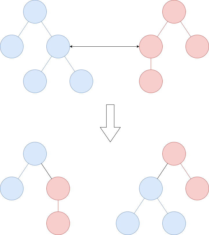
Figure 4: Crossover

3.5 Operator Mutation

An Operator Mutation works the following way: an operator is randomly selected and replaced with a random tree. A new randomly generated subtree is inserted instead of selected operator [2]. Figure 5 illustrates the operator mutation operation.

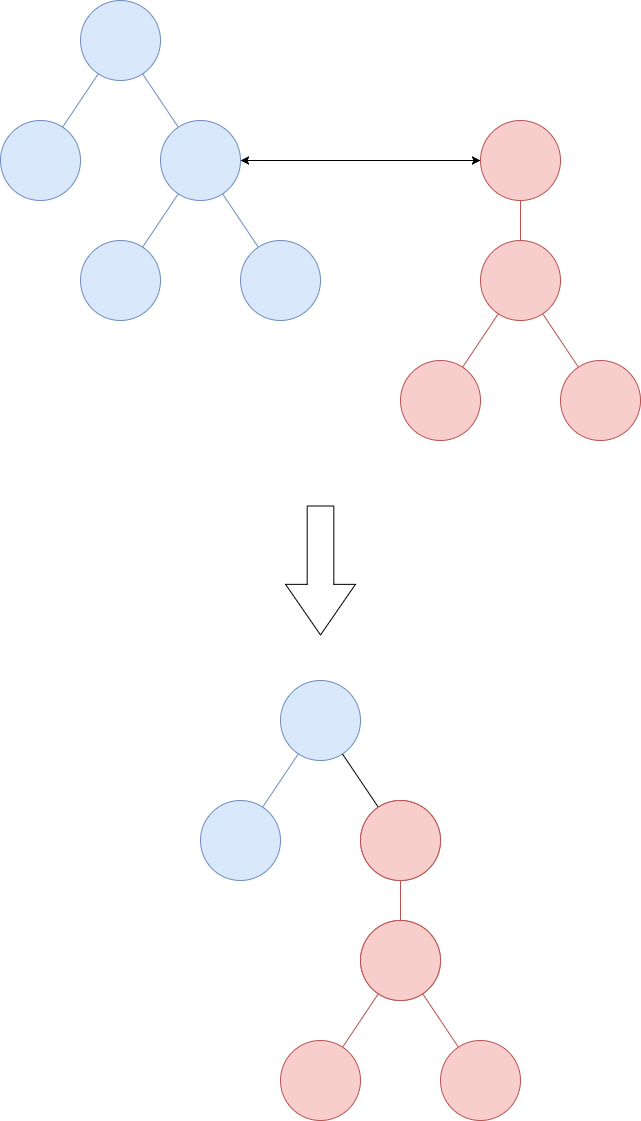
Figure 5: Mutation

3.6 Term Mutation

Term mutation never replaces a term by a random tree. The term mutation is defined as follows:

$$if\;X\;is\;Symbolic,\;then\;X\;is\;replaced\;by\;random\;X_{i}\;i\in[1,n],\;where\;n\;is\;number\;of\;features\;in\;dataset$$

$$if\;X\;is\;Constant,\;then\;X\;is\;replaced\;by\;X+r\;where\;r\;is\;normal\;random\;variable\;(0;\;1)$$

3.7 Mutation Probabilities

During mutation each operator type is being randomly chosen with following probability table:

Operator Type	Probability
Boolean	0.1
Comparison	0.2
Mathematical	0.3
Terms	0.5

3.8 Selection

Rank selection with elite size 1 used as the selection operation [2].

3.9 Evolution Algorithm

Evolution is implemented via canonical genetic algorithm method [5]:

Result: Best individual

1 max_generation = 100;

2 population_size = 100;

3 cx_prob = 0.5;

4 mut_prob = 0.5;

5 population = random_population(population_size);

6 best_ind = select_best(population);

7 generation = 0;

8 while best_ind.fitness < 1 or generation < max_generation do

9       selected_population = selection(population) ;

10       crossed_population = crossover(selected_population, cx_prob) ;

11       mutated_population = mutation(crossed_population, mut_prob) ;

12       population = mutated_population best_ind = select_best(population);

13       generation++;

14      

15 end while

return best_ind

Algorithm 1 GP Classifier Evolution Algorithm

4 Soft Genetic Programming Classifier Design

The main idea of SGP is the usage of weighted continuous functions instead of discontinuous boolean and comparison functions. Weight setting will allow calibrating each operator’s effect in a pseudo logical tree, leading to a more adaptive classifier design.

4.1 Soft Operators

We change boolean and comparison operators to weighted continuous analogs [10] (we will call those function sets pseudo boolean and pseudo comparison operators):

Pseudo Boolean:

Also we will add additional operators:

Pseudo Comparison:

Mathematical:

Also we will add additional nonlinear operators:

Terms:

$$Symbolic:\ \rightarrow X_{i}\;\;\;i\in 1,n,\;where\;n\;-\;number\;of\;features$$

$$Constant:\ \rightarrow\mathbb{R}$$

Weights:

$$Weight:\ \rightarrow w\;,\;where\;w\;is\;random\;variable\;uniformly\;distributed\;on\;[0,1]$$

4.2 Soft Tree Representation

SGP tree is a tree where each pseudo boolean and comparison operator has its weight parameter, as is shown on Figure 6:

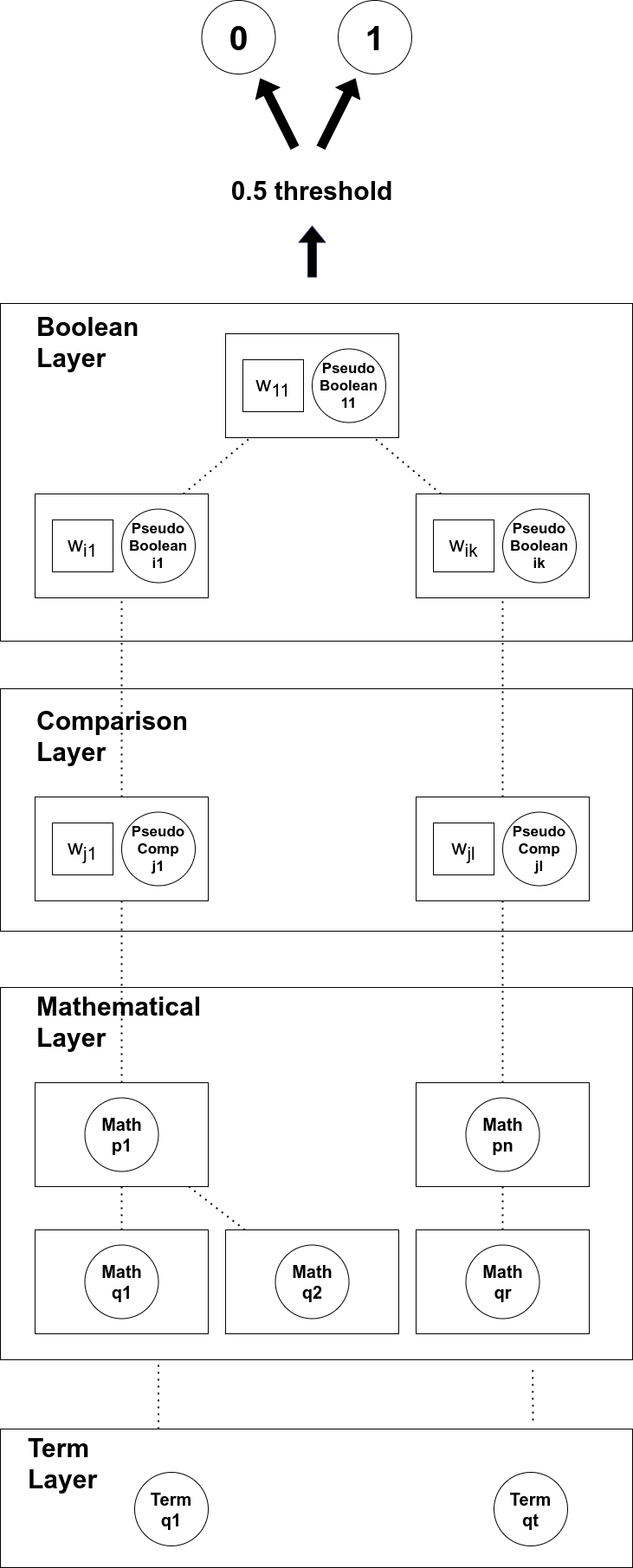
Figure 6: SGP Tree

4.3 Random Tree Generation

See 3.2

4.4 Fitness Function

See 3.3

4.5 Weight Adjustment

In SGP we introduce weight adustment operation:

1procedure weight_adjustment($individual,max\_tries$);

2 for i in max_tries do

3       candidate = copy(individual);

4       coordinate, w = individual.get_random_weight();

5       new_w = w + random_shift();

6       candidate.set_weight(coordinate, new_w);

7       if candidate.fitness > individual.fitness then

8             return candidate

9       end if

10      

11 end for

return individual

Algorithm 2 Weight Adjustment

The main point of weight adjustment operation is to find any positive improvement using weight calibration.

4.6 Fitness Driven Genetic Operations

The main problem of classifier trees is that they have very fragile structures, and the probability of degradation after canonical crossover and mutation operations is to high. In the SGP evolution algorithm, we will use only positive improvement evolution operations.

Positive Crossover doesn’t accept an offsrping which is worse then its parents:

1procedure positive_crossover($ind1,ind2$);

2 child1, child2 = crossover(ind1, ind2);

3 candidate1, candidate2 = max([ind1,ind2,child1,child2], by=fitness, 2);

return [candidate1, candidate2]

Algorithm 3 Positive Crossover

Positive Mutation accepts only those mutations which improves individual’s genome:

1procedure positive_mutation($ind1,max\_tries$);

2 for i in max_tries do

3       mutant = mutate(ind);

4       if mutant.fitness > ind.fitness then

5             return mutant

6       end if

7      

8 end for

return ind

Algorithm 4 Positive Mutation

4.7 Extension Mutation

There is a handy technique for avoiding stucking an improvement of the population in some specific random subspace. A good way of an individual improvement is adding OR operator as tree root with random subtree, as it is shown on the Figure 7.

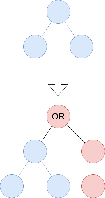
Figure 7: Extension Mutation

The Extension Mutation operation increases the probability of positive genome improvement.

4.8 Multiple Population

The usage of fitness driven crossover and mutation operation provokes the problem of lacking gene variation. This problem is solved using the multiple population technique. On each Nth generation the best individual of each population is "thrown" to the sequent population [13].

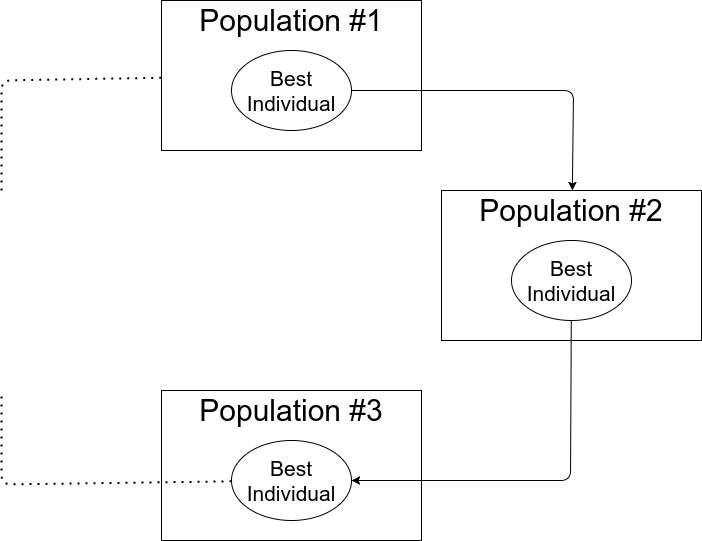
Figure 8: Multiple Population

4.9 Evolution Algorithm

SGP evolution algorithm:

Result: Best individual

1 max_generation = 100;

2 population_size = 100;

3 population_num = 4;

4 cx_prob = 0.5;

5 mut_prob = 0.5;

6

7populations = [] ;

8 for i in population_num do

9       populations[i] = random_population(population_size);

10      

11 end for

12

13best_inds = [] ;

14 for i in population_num do

15       best_inds[i] = select_best(populations[i]);

16      

17 end for

18

19best_ind_ever = max(best_inds, key = ’fitness’)

20generation = 0;

21 while best_ind_ever.fitness < 1 or generation < max_generation do

22       for i in population_num do

23             selected_population = selection(populations[i]) ;

24             crossed_population = crossover(selected_population, cx_prob) ;

25             mutated_population = mutation(crossed_population, mut_prob) ;

26             weighted_population = weight_adjustment(mutated_population) ;

27             extended_population = weight_adjustment(weighted_population) ;

28             populations[i] = extended_population ;

29             best_inds[i] = select_best(populations[i]);

30            

31       end for

32      if generation mod 5 == 0 then

33             for i in population_num do

34                   populations[i+1].append(best_inds[i]);

35                  

36             end for

37            

38       end if

39      best_ind_ever = max(best_inds, key = ’fitness’);

40       generation++;

41      

42 end while

return best_ind_ever

Algorithm 5 SGP Classifier Evolution Algorithm

5 Visualization

Let’s compare the behavior of GP and SGP Classifier on generated 2D datasets [7].

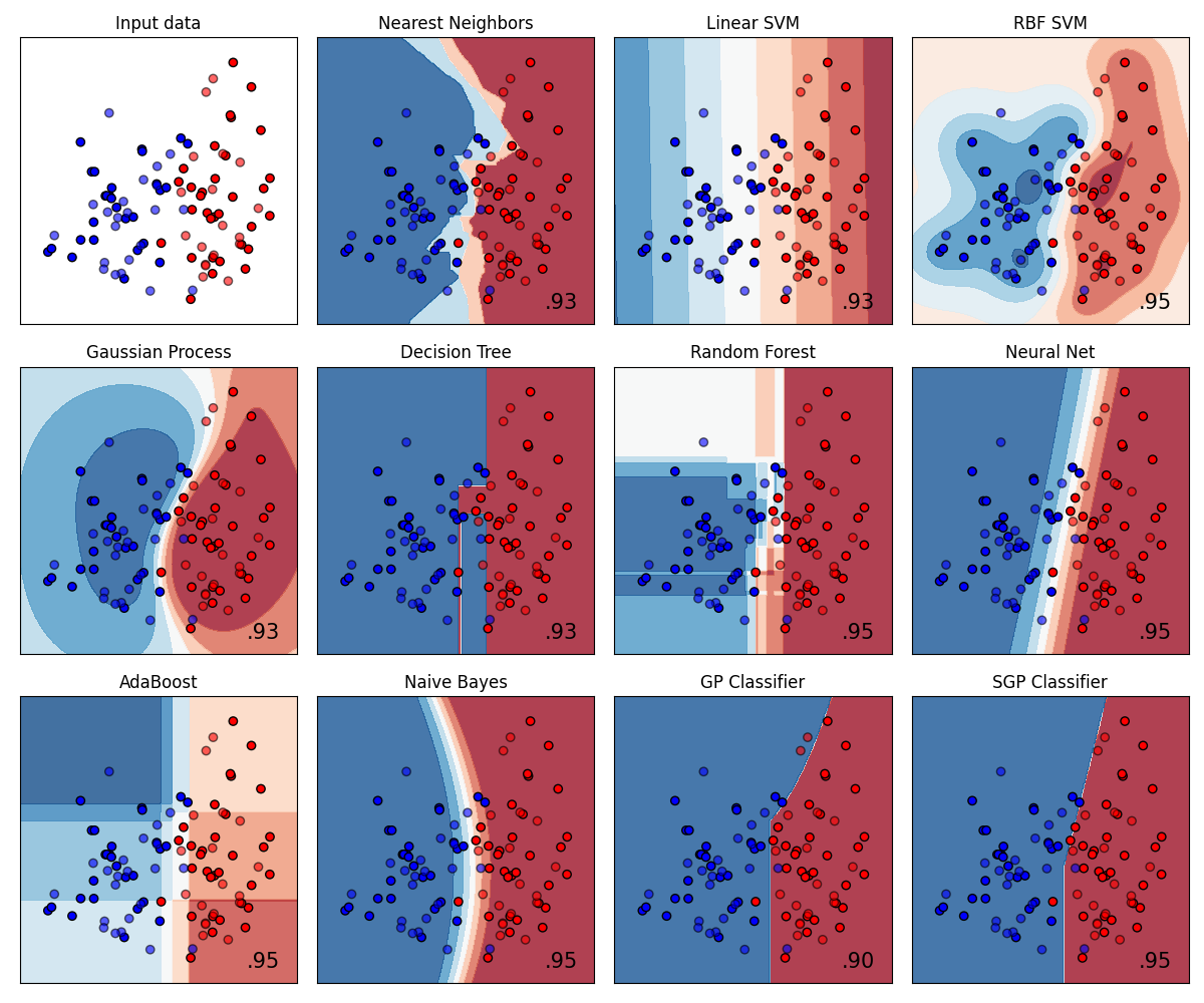
Figure 9: Linearly separable dataset

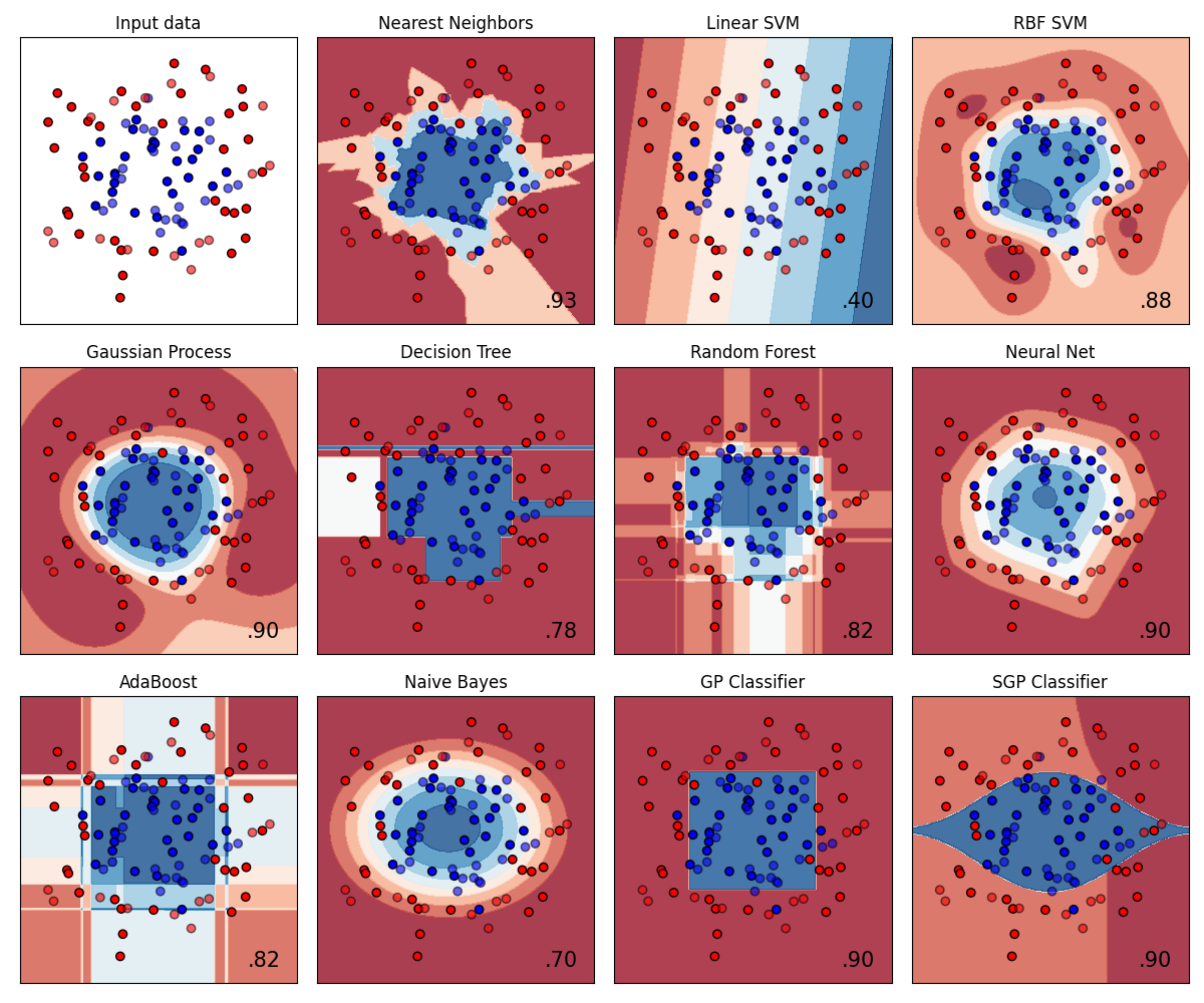
Figure 10: Large circle containing a smaller circle dataset

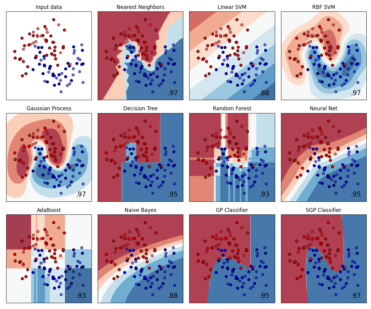
Figure 11: Two interleaving half circles dataset

We can see that both GP and SGP classifiers show confident behavior. As it could be expected, the SGP Classifier tends to use nonlinear dependencies. SGP classifier highly likely have strict borders(i.e. $\mu(\{SGP(x,y)\in]0,1[\ \})\sim 0$), as it is common behavior for Decision Trees.

6 Experimental Results

We have tested SGP and GP classifiers using Large Benchmark Suite [12] for binary classification problem. As a classification quality score we used balanced accuracy.

Test results were gathered by following testing algorithm:

1 for dataset in datasets do

2       for i in [1,20] do

3             shuffledDataset = shuffle(dataset) ;

4             train, test = split(shuffledDataset, .7) ;

5             for cls in classifiers do

6                   cls.fit(train) score = balancedAccuracy(cls, test)

7             end for

8            

9       end for

10      

11 end for

Algorithm 6 Testing algorithm

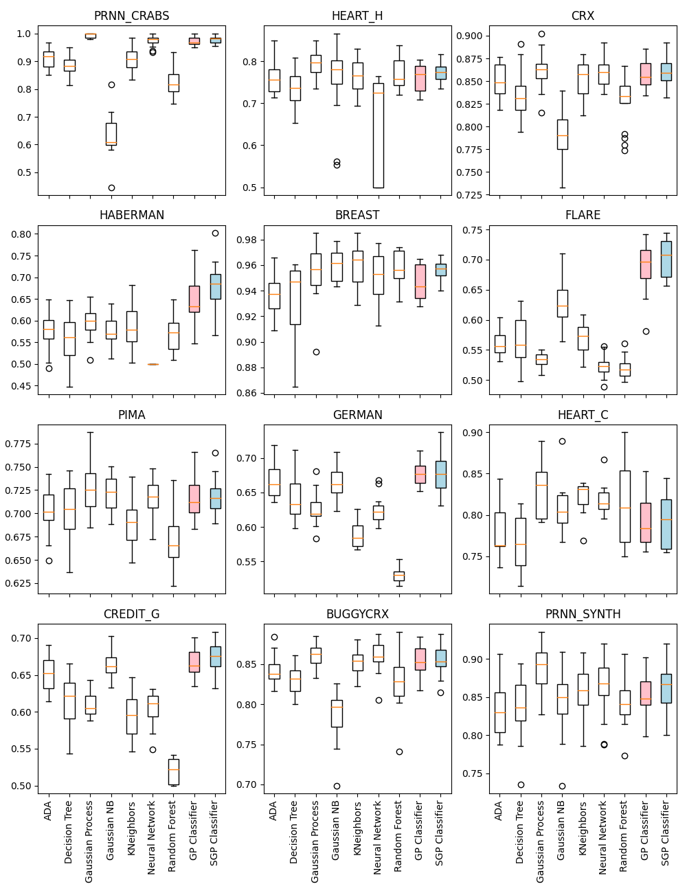
Figure 12: Test Results. GP Classifier - pink, SGP Classifer - blue

Below we provide a heatmap table view with mean balanced accuracy results:

	prnn crabs	heart h	crx	haberman	breast	flare
SGP Classifier	0.978	0.7752	0.7752	0.6792	0.9559	0.7023
GP Classifier	0.9724	0.7597	0.7597	0.6522	0.9464	0.6856
ADA	0.9095	0.7594	0.7594	0.5752	0.9358	0.5613
Decision Tree	0.8815	0.7312	0.7312	0.5585	0.9328	0.5654
Gausian Process	0.994	0.7925	0.7925	0.5981	0.953	0.534
Gausian NB	0.632	0.748	0.745	0.5748	0.9605	0.6305
KNeighbors	0.9079	0.7654	0.7654	0.5857	0.96	0.5727
Neural Network	0.9734	0.6429	0.6429	0.5	0.9517	0.5229
Random Forest	0.8249	0.769	0.769	0.5702	0.958	0.5196

	pima	german	heart c	credit g	buddyCrx	prnn synth
SGP Classifier	0.7181	0.6791	0.7929	0.674	0.8559	0.8642
GP Classifier	0.7176	0.6778	0.7938	0.6668	0.8537	0.8543
ADA	0.703	0.6667	0.782	0.6536	0.8427	0.8342
Decision Tree	0.7009	0.6394	0.7661	0.6151	0.8309	0.8368
Gausian Process	0.7288	0.6255	0.8304	0.6101	0.8614	0.8886
Gausian NB	0.7218	0.6633	0.8127	0.6637	0.7866	0.844
KNeighbors	0.6886	0.588	0.8191	0.5941	0.8517	0.8551
Neural Network	0.7168	0.6255	0.8206	0.6041	0.8598	0.8629
Random Forest	0.6714	0.5297	0.8146	0.5197	0.828	0.846

SGP provides very positive average results, and especially nice at haberman and flare datasets. All results can be regathered running script https://github.com/survexman/sgp_classifier/blob/main/soft/gp_classification.py

7 Conclusion

This survey introduces the concept of Soft Genetic Programming. The robustness of the SGP Classifier is presented. This research aimed to deliver a new genetic programming design with pseudo boolean and pseudo comparison operators and show its quality.

Never the less SGP has several drawbacks:

• Performance issue. SGP training stage takes much more time than classical classifers do.

• An incapability to use SGP as a feature selection tool. Due to the weighted operator design, each branch and operator can have a very low weight. Thus the term that belongs to the weighted operator has low significance and cannot be used as a significant feature. In classical GP Classifier, each symbolic variable highly likely has a high significance degree and can thus be selected as meaningful feature.

Anyway, the improvement of the SGP technique for a particular task can provide excellent practical results.

References

- [1] Chan-Sheng Kuo and T. Hong and Chuen-Lung Chen Applying genetic programming technique in classification trees, 2007 Soft Computing, vol. 11, pages 1165-1172
- [2] Koza, John R. Genetic Programming: On the Programming of Computers by Means of Natural Selection 1992 0-262-11170-5 MIT Press Cambridge, MA, USA
- [3] Bhowan Urvesh, Zhang Mengjie and Johnston Mark Genetic Programming for Classification with Unbalanced Data 2010 Springer Berlin Heidelberg pages 1-13 ISBN: 978-3-642-12148-7
- [4] Emmanuel. Dufourq Data classification using genetic programming, 2015
- [5] D. E. Goldberg Genetic Algorithms in Search, Optimization and Machine Learning Boston, MA, USA: Addison-Wesley Longman Publishing Co., Inc., 1st ed., 1989.
- [6] Suarez Ranyart, Valencia-Ramírez, José and Graff Mario. Genetic programming as a feature selection algorithm. 2014 IEEE International Autumn Meeting on Power, Electronics and Computing, ROPEC 2014. 1-5. 10.1109/ROPEC.2014.7036345. (2014)
- [7] scikit-learn.org Classifier comparison https://scikit-learn.org/stable/auto_examples/classification/plot_classifier_comparison.html
- [8] Silva, Sara and Almeida, Jonas, Dynamic Maximum Tree Depth, Genetic and Evolutionary Computation — GECCO 2003, 1776–1787 Springer Berlin Heidelberg ISSN 978-3-540-45110-5
- [9] Hamed Hatami. Decision trees and influences of variables over product probability spaces, 2006; arXiv:math/0612405.
- [10] O’Donnell Ryan Analysis of Boolean Functions, 2014 Cambridge University Press DOI: 10.1017/CBO9781139814782
- [11] Moulinath Banerjee and Ian W. McKeague. Confidence sets for split points in decision trees, 2007, Annals of Statistics 2007, Vol. 35, No. 2, 543-574; arXiv:0708.1820. DOI: 10.1214/009053606000001415.
- [12] Randal S. Olson, William La Cava, Patryk Orzechowski, Ryan J. Urbanowicz and Jason H. Moore. PMLB: A Large Benchmark Suite for Machine Learning Evaluation and Comparison, 2017; arXiv:1703.00512.
- [13] Søren B. Vilsen, Torben Tvedebrink and Poul Svante Eriksen. DNA mixture deconvolution using an evolutionary algorithm with multiple populations, hill-climbing, and guided mutation, 2020; arXiv:2012.00513.