Regular spiking in high conductance states: the essential role of inhibition

Abstract

Strong inhibitory input to neurons, which occurs in balanced states of neural networks, increases synaptic current fluctuations. This has led to the assumption that inhibition contributes to the high spike-firing irregularity observed in vivo. We used single compartment neuronal models with time-correlated (due to synaptic filtering) and state-dependent (due to reversal potentials) input to demonstrate that inhibitory input acts to decrease membrane potential fluctuations, a result that cannot be achieved with simplified neural input models. To clarify the effects on spike-firing regularity, we used models with different spike-firing adaptation mechanisms and observed that the addition of inhibition increased firing regularity in models with dynamic firing thresholds and decreased firing regularity if spike-firing adaptation was implemented through ionic currents or not at all. This novel fluctuation-stabilization mechanism provides a new perspective on the importance of strong inhibitory inputs observed in balanced states of neural networks and highlights the key roles of biologically plausible inputs and specific adaptation mechanisms in neuronal modeling.

Introduction

In awake animals, neocortical neurons receive a stream of random synaptic inputs arising from background network activity [1, 2, 3]. This “synaptic noise” is responsible for the fluctuations in membrane potential and stochastic nature of spike-firing times [4, 5, 6, 7, 8, 9, 10]. Since spike-firing times encode the information transmitted by neurons, investigating the properties of neuronal responses to stochastic input, representing pre-synaptic spike arrivals, is of significant interest.

Typically, the total conductance of inhibitory synapses is several-fold higher than that of excitatory synapses [11]. This state, commonly referred to as the “high conductance state” has been demonstrated to significantly affect the integrative properties of neurons [12, 13, 14, 15, 2]. Concurrently, the high inhibition-to-excitation ratio introduces additional synaptic noise, which should intuitively result in noisier firing. However, studies have demonstrated that the high ratio of inhibition may lead to more efficient information transmission [16, 17, 18]. In vivo studies have also demonstrated that the onset of stimuli can stabilize the membrane potential without a significant change in its mean value [19, 20]. Monier et al. [19] observed that the decrease in fluctuations was associated with higher evoked inhibition, which may have a shunting effect [21]. Nevertheless, a theoretical framework explaining why and under which conditions this shunting effect overpowers the increased synaptic noise is lacking.

Synaptic input can be modelled as temporary opening of excitatory and inhibitory ion channels, which act to either depolarize or hyperpolarize the neural membrane, respectively. Statistical measures of membrane potential can be calculated exactly with the resulting expressions being non-analytic [22] or they can be approximated in the steady-state with the effective time-constant approximation [23, 24]. For better analytical tractability, the synaptic drive is often simplified with one (or both) of the following assumptions:

1. The magnitude of the synaptic current elicited by each presynaptic spike is independent of the voltage [25, 26, 27, 28, 29, 30], or

2. Time profiles of individual synapses (synaptic filtering) are neglected [8, 23, 31, 32, 33, 30, 34].

In order to observe the shunting effect of inhibition [19], reversal potentials have to be considered, which excludes assumption A1. Richardson [23] demonstrated that an increase in inhibition could decrease the membrane potential for strongly hyperpolarized membranes in a model of synaptic input with omitted synaptic filtering (assumption A2). However, we demonstrate that if neither of the simplifying assumptions are used, the membrane potential stabilization effect can be observed across the complete range of membrane potentials, despite increased synaptic current fluctuations (Fig 1A,B).

This naturally poses the question if the decreased membrane potential fluctuations lead to more regular firing activity [20]. To this end, we analyze the effect of membrane potential stabilization on different neuronal models. In particular, we focus on how the effects of inhibition change for different spike-firing adaptation (SFA) mechanisms. SFA is responsible for the decrease of a neuron’s firing rate in response to a sustained stimulus and plays a crucial role in all stages of sensory processing (e.g., [35, 36, 37, 38, 39, 40]). We compare two distinct SFA mechanisms: adaptation through ionic currents (muscarinic currents, AHP currents) and adaptation through dynamic threshold. We demonstrate that despite their formal similarities [41, 42] the effect of inhibition qualitatively differs for these SFA mechanisms (Fig 1C,D). We illustrate the differences on the analytically more tractable generalized leaky integrate-and-fire models (GLIF) followed by the biophysically more plausible Hodgkin-Huxley (HH)-type models.

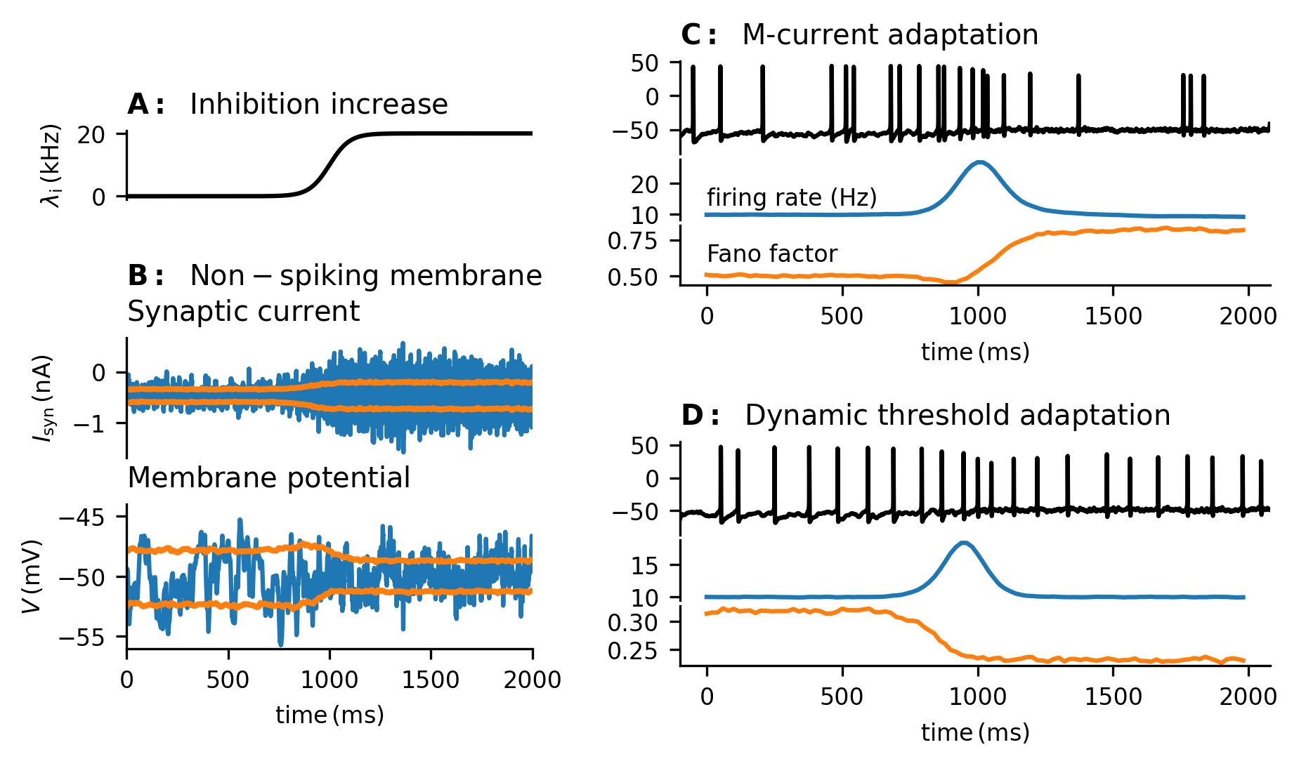
Figure 1: A: During a $2\text{\,}\mathrm{s}$ long simulation, the intensity of inhibitory input increases from $0\text{\,}\mathrm{kHz}$ to $20\text{\,}\mathrm{kHz}$. The pre-synaptic spike trains are modeled as Poisson point processes. B: The intensity of excitatory input is increased simultaneously with the inhibition in order to maintain the mean membrane potential constant. This increases fluctuations of the synaptic current but decreases fluctuations of the membrane potential. The orange lines signify the mean value $\pm$ standard deviation. C and D: The effect of membrane potential stabilization on firing regularity. The intensity of the inhibitory input follows the time course shown in A, and the intensity of the excitatory activity is increased in order to maintain the steady state post-synaptic firing rate at approximately $10\text{\,}\mathrm{Hz}$ (blue trace). The firing regularity (measured here by the Fano factor, orange trace) decreases with the addition of inhibition to the input in the model with spike-firing adaptation by M currents (C). However, the model with dynamic threshold (D) exhibits a clear increase in regularity with the added inhibitory input. The mean firing rate and Fano factor were calculated by a sliding window of length $100\text{\,}\mathrm{ms}$ from approximately $10^{5}$ trials.

Methods

Subthreshold membrane potential

In order to analyze the behavior of neurons in the absence of any spike-firing mechanism, we consider a point neuronal model with membrane potential $V$ described by

$$C\frac{\mathrm{d}V(t)}{\mathrm{d}t}=-g_{\mathrm{L}}(V(t)-E_{\mathrm{L}})+\frac{1}{a}(I_{\mathrm{e}}(t)+I_{\mathrm{i}}(t)),$$ (1)

where $C$ is the specific capacitance of the membrane, $g_{\mathrm{L}}$ is the specific leak conductance, $E_{\mathrm{L}}$ is the leakage potential, $I_{\mathrm{e},\mathrm{i}}$ are the synaptic currents due to stimulation by afferent neurons through excitatory and inhibitory synapses, respectively, and $a$ is the membrane area [43, 44]. For brevity, we will further use $V\equiv V(t)$. The synaptic currents are described by

$$I_{\mathrm{e},\mathrm{i}}(t)=g_{\mathrm{e},\mathrm{i}}(t)(V-E_{\mathrm{e},\mathrm{i}}),$$ (2)

where $g_{\mathrm{e}}(t)$, $g_{\mathrm{i}}(t)$ are the total excitatory and inhibitory conductances, and $E_{\mathrm{e}}$, $E_{\mathrm{i}}$ are the respective synaptic reversal potentials.

The total conductances in the Eq (2) are given by

$$g_{\mathrm{e},\mathrm{i}}(t)=\sum_{t_{k}\in\mathcal{T}_{\mathrm{e},\mathrm{i}}}h_{\mathrm{e},\mathrm{i}}(t-t_{k}),$$ (3)

where $\mathcal{T}_{\mathrm{e},\mathrm{i}}$ are sets of presynaptic spike times modeled as realizations of stochastic point processes and $h_{\mathrm{e},\mathrm{i}}$ are filtering functions (i.e., time profiles of individual excitatory and inhibitory conductances).

Unless stated otherwise, we used the following parameters: $C=$1\text{\,}\mathrm{\SIUnitSymbolMicro}\mathrm{F}\mathrm{/}\mathrm{c}\mathrm{m}^{2}$$, $g_{\mathrm{L}}=$0.045\text{\,}\mathrm{m}\mathrm{S}\mathrm{/}\mathrm{c}\mathrm{m}^{2}$$, $E_{\mathrm{L}}=$-80\text{\,}\mathrm{mV}$$, $E_{\mathrm{e}}=$0\text{\,}\mathrm{mV}$$, $E_{\mathrm{i}}=$-75\text{\,}\mathrm{mV}$$, $a=$3.4636\text{\times}{10}^{-4}\text{\,}\mathrm{c}\mathrm{m}^{2}$$ [45].

Spike firing models

GLIF models

We consider three versions of the GLIF model:

1. The classical Leaky Integrate-and-Fire model (LIF),

2. LIF with SFA through ionic (after-hyperpolarization) currents (AHP-LIF),

3. LIF with SFA through dynamic threshold (DT-LIF).

The membrane potential of the LIF model obeys the Eq (1). Whenever $V>\theta$, where $\theta$ is a fixed threshold value, a spike is fired, and the membrane potential $V$ is reset to a value $V_{r}$. For our simulations, we used $\theta=$-55\text{\,}\mathrm{mV}$$ and $V_{r}=E_{\mathrm{L}}$.

In the model with AHP current SFA (AHP-LIF), an additional hyperpolarizing conductance $g_{\mathrm{AHP}}$ is included in the model, and the membrane potential then obeys the equation [46, 47, 48]:

$$C\frac{\mathrm{d}V}{\mathrm{d}t}=-g_{\mathrm{L}}(V-E_{\mathrm{L}})-g_{\mathrm{AHP}}(t)(V-E_{\mathrm{K}})+I_{\mathrm{e}}(t)+I_{\mathrm{i}}(t),$$ (4)

or equivalently

$$\tau_{\mathrm{ef}}^{\mathrm{AHP}}\frac{\mathrm{d}V}{\mathrm{d}t} =-(V-V_{\mathrm{ef}}^{\mathrm{AHP}}),$$ (5)

$$\tau_{\mathrm{ef}}^{\mathrm{AHP}}(t) =\frac{aC}{g_{\mathrm{e}}(t)+g_{\mathrm{i}}(t)+g_{\mathrm{AHP}}(t)+ag_{\mathrm{L}}},$$ (6)

$$V_{\mathrm{ef}}^{\mathrm{AHP}}(t) =\frac{ag_{\mathrm{L}}E_{\mathrm{L}}+g_{\mathrm{e}}(t)E_{\mathrm{e}}+g_{\mathrm{i}}(t)E_{\mathrm{i}}+g_{\mathrm{AHP}}(t)E_{\mathrm{K}}}{g_{\mathrm{e}}(t)+g_{\mathrm{i}}(t)+g_{\mathrm{AHP}}(t)+ag_{\mathrm{L}}}.$$ (7)

where $E_{\mathrm{K}}$ is the potassium reversal potential, and $g_{\mathrm{AHP}}$ is the corresponding conductance which increases by $\Delta g_{\mathrm{AHP}}$ when a spike is fired and otherwise decays exponentially to zero with a time constant $\tau_{\mathrm{AHP}}$. $V_{\mathrm{ef}}^{\mathrm{AHP}}$ then represents the effective reversal potential. Note that for simplicity, we omitted the voltage dependence of $g_{\mathrm{AHP}}$.

In the dynamic threshold model (DT-LIF), the threshold increases by $\Delta\theta$ after each spike and then decreases exponentially to $\theta_{0}$ with time constant $\tau_{\theta}$.

The parameters for the GLIF models are specified in the Tab. 1.

Table 1: GLIF models parameters

	LIF	AHP-LIF	DT-LIF
$\theta$, $\theta_{0}$ ($\mathrm{mV}$)	-50	-50	-50
$\tau_{\mathrm{AHP}}$ ($\mathrm{ms}$)	-	100	-
$\Delta g_{\mathrm{AHP}}$ ($\mathrm{nS}$)	0	5	0
$E_{\mathrm{K}}$ ($\mathrm{mV}$)	-	-100	-
$\tau_{\theta}$ ($\mathrm{ms}$)	-	-	100
$\Delta_{\theta}$ ($\mathrm{mV}$)	0	0	4

Hodgkin-Huxley models

We adopted HH-type models developed by Destexhe et al. [49]. The membrane potential obeys the equation:

$$\begin{split}C\frac{\mathrm{d}V}{\mathrm{d}t}=&-g_{\mathrm{L}}(V-E_{\mathrm{L}})-g_{\mathrm{Na}}m^{3}h(V-E_{\mathrm{Na}})-\\ &-g_{\mathrm{K}}n^{4}(V-E_{\mathrm{K}})-g_{\mathrm{M}}p(V-E_{\mathrm{K}})-\frac{1}{a}I_{\mathrm{syn}},\end{split}$$ (8)

where $E_{\mathrm{Na}}$ and $E_{\mathrm{K}}$ are the sodium and potassium reversal potentials, respectively; $g_{\mathrm{Na}}$, $g_{\mathrm{K}}$, and $g_{\mathrm{M}}$ are peak conductances; and $m$, $h$, $n$, and $p$ are gating variables obeying the equation:

$$\frac{\mathrm{d}x}{\mathrm{d}t}=\alpha_{x}(V)(1-x)-\beta_{x}(V)x,$$ (9)

or equivalently:

$$\tau_{x}(V)\frac{\mathrm{d}x}{\mathrm{d}t}=-(x-x_{\infty}(V)),$$ (10)

where $x$ is the respective gating variable, $\alpha_{x}$ and $\beta_{x}$ are the activation and inactivation functions, respectively, and

$$\tau_{x}(V) =\frac{1}{\alpha_{x}(V)+\beta_{x}(V)},$$ (11)

$$x_{\infty}(V) =\frac{\alpha_{x}(V)}{\alpha_{x}(V)+\beta_{x}(V)}.$$ (12)

The activation and inactivation functions are defined as follows:

$$\alpha_{m} =-0.32\frac{V-V_{T}-13}{\exp(-(V-V_{T}-13)/4)-1},$$ (13)

$$\beta_{m} =0.28\frac{V-V_{T}-40}{\exp((V-V_{T}-40)/5)-1},$$ (14)

$$\alpha_{h} =A_{h}\exp(-(V-V_{T}-V_{S}-17)/18),$$ (15)

$$\beta_{h} =\frac{4}{1+\exp(-(V-V_{T}-V_{S}-40)/5)},$$ (16)

$$\alpha_{n} =-0.032\frac{V-V_{T}-15}{\exp(-(V-V_{T}-15)/5)-1},$$ (17)

$$\beta_{n} =0.5\exp(-(V-V_{T}-10)/40),$$ (18)

$$\alpha_{p} =0.0001\frac{V+30}{1-\exp(-(V+30)/9)},$$ (19)

$$\beta_{p} =-0.0001\frac{V+30}{1-\exp((V+30)/9)}.$$ (20)

Table 2: Parameters of the HH models

	HH-0	HH-M	HH-DT
$g_{\mathrm{Na}}$ ($\mathrm{m}\mathrm{S}\mathrm{/}\mathrm{c}\mathrm{m}^{2}$)	50	50	50
$g_{\mathrm{K}}$ ($\mathrm{m}\mathrm{S}\mathrm{/}\mathrm{c}\mathrm{m}^{2}$)	5	5	5
$g_{\mathrm{M}}$ ($\mathrm{m}\mathrm{S}\mathrm{/}\mathrm{c}\mathrm{m}^{2}$)	0	0.5	0
$E_{\mathrm{Na}}$ ($\mathrm{mV}$)	50	50	50
$E_{\mathrm{K}}$ ($\mathrm{mV}$)	-90	-90	-90
$V_{T}$ ($\mathrm{mV}$)	-58	-58	-58
$V_{S}$ ($\mathrm{mV}$)	-10	-10	14
$A_{h}$ ($\mathrm{m}\mathrm{s}^{-1}$)	0.128	0.128	0.00128

We set $g_{M}=0$ in both the HH-0 and HH-DT models, and $g_{M}>0$ in the HH-M model. In order to achieve dynamic threshold behavior, we modified the activation and deactivation functions of the gating variable $h$, which is responsible for deactivating voltage-gated sodium channels after firing a spike, by changing the parameters $A_{h}$ and $V_{S}$. For more details see the Supplementary Figure 1.

The parameters for the three HH-type models (without SFA (HH-0) / M-current SFA (HH-M) / dynamic threshold SFA (HH-DT)) are specified in the Tab 2.

Simulation details

For synapses, we used the exponential filtering function:

$$h_{\mathrm{e},\mathrm{i}}(t)=\begin{cases}A_{\mathrm{e},\mathrm{i}}\exp(-t/\tau_{\mathrm{e},\mathrm{i}})\ \ \ t\geq 0\\ 0\ \ \ t<0\end{cases}$$ (21)

with $A_{\mathrm{e}}=A_{\mathrm{i}}=$0.0015\text{\,}\mathrm{\SIUnitSymbolMicro S}$$, $\tau_{\mathrm{e}}=$3\text{\,}\mathrm{ms}$$, $\tau_{\mathrm{e}}=$10\text{\,}\mathrm{ms}$$. Such input parameters with intensities $\lambda_{\mathrm{e}}=$2.67\text{\,}\mathrm{Hz}$$ and $\lambda_{\mathrm{i}}=$3.73\text{\,}\mathrm{kHz}$$ provide an input with $g_{\mathrm{e}}^{0}=$12\text{\,}\mathrm{nS}$$, $\sigma_{\mathrm{e}}=$3\text{\,}\mathrm{nS}$$, $g_{\mathrm{i}}^{0}=$57\text{\,}\mathrm{nS}$$, and $\sigma_{\mathrm{i}}=$6.6\text{\,}\mathrm{nS}$$, as reported by Destexhe et al. [45].

To ensure stability of the computation, we used the following update rule for the simulations:

$$V_{n+1} =\left(V_{\mathrm{ef}}\right)_{n+1}+\left(V_{n}-\left(V_{\mathrm{ef}}\right)_{n+1}\right)\exp\left(\frac{\Delta t}{\tau_{n+1}}\right),$$ (22)

$$V_{\mathrm{ef}} =\frac{\sum_{x\in X}g_{x}E_{x}}{\sum_{x\in X}g_{x}}$$ (23)

$$\tau_{\mathrm{ef}} =\frac{C}{\sum_{x\in X}g_{x}}$$ (24)

where $X$ contains all the channel types (synaptic, leak, voltage-gated, and adaptive). The update rule for the synaptic conductances $g_{\mathrm{e},\mathrm{i}}$ was

$$\left(g_{\mathrm{e},\mathrm{i}}\right)_{n+1}=\left(g_{\mathrm{e},\mathrm{i}}\right)_{n}\exp\left(\frac{\Delta t}{\tau_{\mathrm{e},\mathrm{i}}}\right)+N_{\mathrm{e},\mathrm{i}}A_{\mathrm{e},\mathrm{i}},$$ (25)

where $\left(N_{\mathrm{e},\mathrm{i}}\right)$ is a Poisson random variable with mean $\lambda_{\mathrm{e},\mathrm{i}}\Delta t$.

We used the step size $\Delta t=$0.025\text{\,}\mathrm{ms}$$.

Evaluating firing rate regularity

A classical measure of the firing regularity of steady spike trains is the coefficient of variation ($\mathrm{C}_{\mathrm{V}}$), defined as follows (e.g., [50]):

$$\mathrm{C}_{\mathrm{V}}{}=\frac{\sigma_{\mathrm{ISI}}}{\mu_{\mathrm{ISI}}},$$ (26)

where $\mu_{\mathrm{ISI}}$ and $\sigma_{\mathrm{ISI}}$ are the mean and standard deviation of the interspike intervals (ISIs), respectively. Lower $\mathrm{C}_{\mathrm{V}}$ indicates higher firing regularity.

To achieve an accurate estimate of the $\mathrm{C}_{\mathrm{V}}$, we estimated the statistics from approximately 160,000 ISIs for each data point. For a Poisson process ($\mathrm{C}_{\mathrm{V}}{}=1$) with this number of ISIs, the estimate of $\mathrm{C}_{\mathrm{V}}{}$ falls within $[0.995,1.005]$ in over 95% of cases. Note that the estimation was more accurate for lower values of $\mathrm{C}_{\mathrm{V}}{}$.

Results

Membrane potential is stabilized with increased input fluctuations

Since the inputs to a neuron consist of pooled spike trains from a large number of presynaptic neurons, according to the Palm-Khintchine theorem [51], it is sufficient to approximate the excitatory and inhibitory inputs by Poisson processes with intensities $\lambda_{\mathrm{e}}$ and $\lambda_{\mathrm{i}}$, respectively [43]. It has been demonstrated that this condition is not necessarily satisfied for neurons in vivo [52]. However, as we discuss below, this should not affect the conclusions of our analysis. According to Campbell’s theorem [53], it then holds for the mean $g_{\mathrm{e},\mathrm{i}}^{0}$ and variance $\sigma^{2}_{\mathrm{e},\mathrm{i}}$ of the input

$$g_{\mathrm{e},\mathrm{i}}^{0} =\lambda_{\mathrm{e},\mathrm{i}}\int_{0}^{\infty}h_{\mathrm{e},\mathrm{i}}(t)\,\mathrm{d}t,$$ (27)

$$\sigma_{\mathrm{e},\mathrm{i}}^{2} =\lambda_{\mathrm{e},\mathrm{i}}\int_{0}^{\infty}h_{\mathrm{e},\mathrm{i}}^{2}(t)\,\mathrm{d}t.$$ (28)

Therefore $\frac{\sigma_{\mathrm{e},\mathrm{i}}}{g_{\mathrm{e},\mathrm{i}}^{0}}=O\left(\frac{1}{\sqrt{\lambda_{\mathrm{e},\mathrm{i}}}}\right)$ (a well-known property of the Poisson shot noise [43])lne:wellknown.

For the purposes of our analysis, we consider the voltage equations of a membrane without any spike-generating mechanism as:

$$\tau_{\mathrm{ef}}(g_{\mathrm{e}}(t),g_{\mathrm{i}}(t))\frac{\mathrm{d}V}{\mathrm{d}t} =-V-V_{\mathrm{ef}}(g_{\mathrm{e}}(t),g_{\mathrm{i}}(t)),$$ (29)

$$\tau_{\mathrm{ef}}(g_{\mathrm{e}},g_{\mathrm{i}}) =\frac{aC}{ag_{\mathrm{L}}+g_{\mathrm{e}}+g_{\mathrm{i}}},$$ (30)

$$V_{\mathrm{ef}}(g_{\mathrm{e}},g_{\mathrm{i}}) =\frac{ag_{\mathrm{L}}E_{\mathrm{L}}+g_{\mathrm{e}}E_{\mathrm{e}}+g_{\mathrm{i}}E_{\mathrm{i}}}{g_{\mathrm{L}}+g_{\mathrm{e}}+g_{\mathrm{i}}}.$$ (31)

For large inputs $\frac{\sigma_{\mathrm{e},\mathrm{i}}}{g_{\mathrm{e},\mathrm{i}}^{0}}\ll 1$, we can linearize the Eq (31):

$$V_{\mathrm{ef}}(g_{\mathrm{e}},g_{\mathrm{i}})\doteq E_{0}\left(1-\frac{g_{\mathrm{e}}^{\mathrm{F}}+g_{\mathrm{i}}^{\mathrm{F}}}{ag_{\mathrm{L}}+g_{\mathrm{e}}^{0}+g_{\mathrm{i}}^{0}}\right)+\frac{g_{\mathrm{e}}^{\mathrm{F}}E_{\mathrm{e}}+g_{\mathrm{i}}^{\mathrm{F}}E_{\mathrm{i}}}{ag_{\mathrm{L}}+g_{\mathrm{e}}^{0}+g_{\mathrm{i}}^{0}},$$ (32)

where $E_{0}=V_{\mathrm{ef}}(g_{\mathrm{e}}^{0},g_{\mathrm{i}}^{0})$ and $g_{\mathrm{e},\mathrm{i}}^{\mathrm{F}}=g_{\mathrm{e},\mathrm{i}}-g_{\mathrm{e},\mathrm{i}}^{0}$. Since the fluctuating terms in Eq (32) disappear with growing input, evaluating the limits with a fixed inhibition-to-excitation ratio $c=\frac{g_{\mathrm{i}}^{0}}{g_{\mathrm{e}}^{0}}$ leads to:

$$\lim_{\lambda_{\mathrm{e}},\lambda_{\mathrm{i}}\rightarrow\infty}\mathrm{E\left[V_{\mathrm{ef}}\right]}=V_{\infty}(c)\equiv\frac{E_{\mathrm{e}}+cE_{\mathrm{i}}}{1+c},$$ (33)

$$\lim_{\lambda_{\mathrm{e}},\lambda_{\mathrm{i}}\rightarrow\infty}\mathrm{Var\left[V_{\mathrm{ef}}\right]}=0.$$ (34)

lne:upperbound_start$\mathrm{Var\left[V_{\mathrm{ef}}\right]}$ is an upper bound on the variance of $V$ (it follows from the Eq (29) that the membrane potential $V$ is essentially a “low-pass filtered” effective reversal potential $V_{\mathrm{ef}}$). Therefore, it also holds that $\lim\limits_{\lambda_{\mathrm{e}},\lambda_{\mathrm{i}}\rightarrow\infty}\mathrm{\langle V\rangle}=V_{\infty}(c)\equiv\frac{E_{\mathrm{e}}+cE_{\mathrm{i}}}{1+c}$ and $\lim\limits_{\lambda_{\mathrm{e}},\lambda_{\mathrm{i}}\rightarrow\infty}\mathrm{\sigma_{V}}=0$lne:upperbound_end. This can also be observed from the perturbative approach suggested in [54] and further developed in [23, 24]. Therefore, any membrane potential between the reversal potentials $E_{\mathrm{i}}$, $E_{\mathrm{e}}$ can be asymptotically reached with zero variance, despite the variance of the total synaptic current $I_{\mathrm{syn}}=I_{\mathrm{e}}+I_{\mathrm{i}}$ increasing. Note that the Poisson condition can be relaxed, since it is sufficient for this result that $\frac{\sigma_{\mathrm{e},\mathrm{i}}}{g_{\mathrm{e},\mathrm{i}}^{0}}\rightarrow 0$ lne:poisson.

lne:star_explainLet $\sigma_{V}(\langle V\rangle;c)$ be the function specifying the standard deviation of the membrane potential with mean $\langle V\rangle$, parametrized by $c$. It is a continuous function, with $\sigma_{V}(E_{\mathrm{L}};c)=\sigma_{V}(V_{\infty}(c);c)=0$, otherwise $\sigma_{V}(\langle V\rangle;c)>0$. Note that lower $c$ leads to higher $V_{\infty}(c)$. Therefore, given $c_{1}>c_{2}$, there has to be an interval close to $V_{\infty}(c_{1})$ where $c_{2}$ results in lower membrane fluctuations. Moreover, simulations indicate that this holds, even in non-limit regimes (Fig 2A, top panel). lne:highchighinh_startThis result is rather counter-intuitive, since with an increase in $c$, it is necessary to increase both $\lambda_{\mathrm{e}}$ and $\lambda_{\mathrm{i}}$ (if $\langle V\rangle>E_{\mathrm{i}}$), and thus simultaneously increase synaptic current fluctuations (Fig 2A, bottom panel) in order to keep the membrane potential constantlne:highchighinh_end. With our choice of parameters, lower $c$ may also result in a slight decrease in membrane potential fluctuations. This is mainly due to the membrane time constant $\tau=\frac{C}{g_{\mathrm{L}}}\doteq$22\text{\,}\mathrm{ms}$$. The shorter the time constant, the closer $V$ follows $V_{\mathrm{ef}}$, and the smaller the region in which decreasing $c$ leads to lower membrane potential variability (see the Supplementary Figure 2)lne:stop_explain.

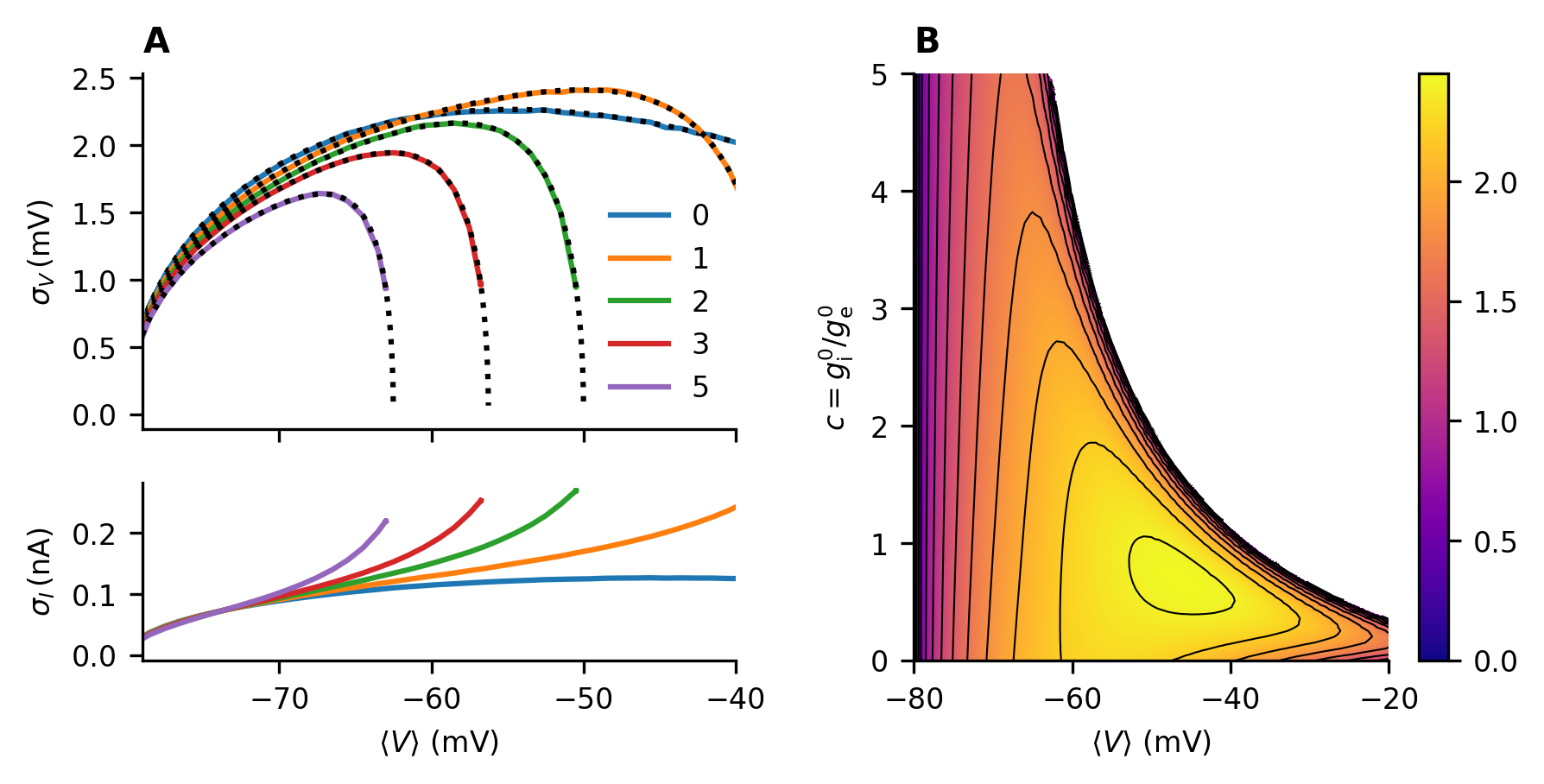
Figure 2: Stabilization of the membrane potential. A, top panel: Membrane potential fluctuations as a function of the mean membrane potential for different values of $c$. The full lines represent data obtained from simulations with different excitatory input intensities $\lambda_{\mathrm{e}}$. The dotted lines represent the effective time-constant approximation (ETA, Appendix A). Bottom panel: The standard deviation $\sigma_{I}$ of the total synaptic current $I_{\mathrm{syn}}=I_{\mathrm{e}}+I_{\mathrm{i}}$. Note that $\sigma_{V}$ decreases with growing $c$ even though $\sigma_{I}$ increases. B: Overview of $\sigma_{V}$ (color) for all achievable $\langle V\rangle$ ($x$-axis) at given $c$ ($y$-axis). $C=$1\text{\,}\mathrm{\SIUnitSymbolMicro}\mathrm{F}\mathrm{/}\mathrm{c}\mathrm{m}^{2}$$ and $g_{\mathrm{L}}=$0.045\text{\,}\mathrm{m}\mathrm{S}\mathrm{/}\mathrm{c}\mathrm{m}^{2}$$, approximation of $\sigma_{V}$ computed from the ETA. Heatmaps for different values of $g_{\mathrm{L}}$ are provided in the Supplementary Figure 2 and for different values of $A_{\mathrm{i}}$ (Eq. (21)) in the Supplementary Figure 3.

Effects on firing regularity

The regularity of spike-firing is important for information transmission between neurons [55, 56, 57, 58]. In the previous section, we demonstrated that if appropriate synaptic drive is used, higher inhibitory input rates (or equivalently higher inhibition-to-excitation ratio $c$) lead to lower membrane potential fluctuations. In this section, we focus on the effects of inhibition on post-synaptic firing regularity, particularly on the regularity of a post-synaptic spike train with a fixed frequency evoked by different stimuli with different levels of inhibition.

Generalized Leaky Integrate-and-Fire models

For our analysis, it is essential to distinguish two different input regimes: 1. Sub-threshold regime: $E_{0}\leq\theta$ and 2. Supra-threshold regime: $E_{0}>\theta$, where $\theta$ is the firing threshold.

In the sub-threshold regime, firing activity is driven by fluctuations in the membrane potential. Therefore, increasing the input rates $\lambda_{\mathrm{e}}$, $\lambda_{\mathrm{i}}$ and simultaneously keeping $E_{0}$ constant leads to a decrease in firing rate due to suppressed membrane potential fluctuations (note that an analogous effect was described in the Hodgkin-Huxley model [59]). In order to maintain the post-synaptic firing rate (PSFR) constant while increasing the input rates, it is necessary to compensate for the decrease in fluctuations by increasing $E_{0}$. Therefore, it is not intuitively clear whether the decrease in membrane potential fluctuations will lead to an increase in firing regularity.

In the supra-threshold regime, the firing activity is given by the driving force on the membrane potential $(V-V_{\mathrm{ef}})/\tau_{\mathrm{ef}}$. Fluctuations in the interspike intervals are then given mostly by the fluctuations of $V_{\mathrm{ef}}$. However, lower fluctuations of $V_{\mathrm{ef}}$ are associated with lower $\tau_{\mathrm{ef}}$ and it is necessary to decrease $E_{0}$, if one wishes to decrease the fluctuations of $V_{\mathrm{ef}}$ and keep the firing rate constant at the same time. Intuitively, the fluctuations of $V_{\mathrm{ef}}$ will impact the firing regularity more, if the difference $(V-V_{\mathrm{ef}})$ is lower. Therefore it is again unclear how the increased synaptic fluctuations affect the firing regularity.

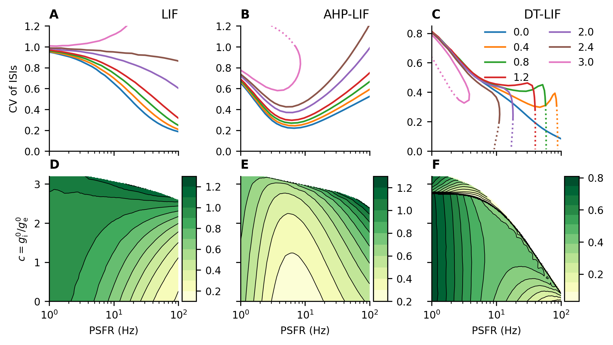
Figure 3: The effect of membrane potential stabilization on spiking regularity in the GLIF models. A-C: Dependence of the $\mathrm{C}_{\mathrm{V}}$ of ISIs on the post-synaptic firing rate for different values of $c$ (color-coded). The dotted parts of the curves represent the sections where $\lambda_{\mathrm{e}}>$100\text{\,}\mathrm{kHz}$$. In the LIF and AHP-LIF model, higher $c$ universally leads to higher $\mathrm{C}_{\mathrm{V}}$. In contrast, in the DT-LIF model, higher $c$ can lead to more regular spike trains, especially if the input intensities are high. If $V_{\infty}(c)\leq\theta$ (or $\theta_{0}$ for the DT-LIF model, i.e., $c\geq 2.75$), the firing rate will eventually drop to 0. D-E: Contour plots with color-coded $\mathrm{C}_{\mathrm{V}}$, $c$ on the $y$-axis. If more than one input can produce the same PSFR with the same $c$, the lowest possible value of $\mathrm{C}_{\mathrm{V}}$ is color-coded, resulting in the discontinuity in F. The data points were obtained from simulations with different input intensities $\lambda_{\mathrm{e}}$, $\lambda_{\mathrm{i}}$.

In general, we observe that in the suprathreshold regime, the $\mathrm{C}_{\mathrm{V}}$ of ISIs decreases with growing PSFR (Fig 3A,D). Moreover, as we show in the Appendix B:

$$\lim_{\lambda_{\mathrm{e}},\lambda_{\mathrm{i}}\rightarrow\infty}\mathrm{C}_{\mathrm{V}}{}=0$$ (35)

However, if the firing rate is held constant, the $\mathrm{C}_{\mathrm{V}}$ increases with growing $c$. Therefore, an increase in the inhibition-to-excitation ratio decreases firing regularity, despite the stabilizing effect on membrane potential.

With high values of $c$, the $\mathrm{C}_{\mathrm{V}}$ grows locally with increasing firing rate. This is due to the fact that as $E_{0}$ is very close to the threshold and the membrane time constant (Eq (30)) is very low, the neuron fires very rapidly (bursts) when $V_{\mathrm{ef}}$ (Eq (29)) exceeds the threshold but is otherwise silent.

For the AHP-LIF model, no improvements are observed in the firing regularity with increasing $c$ (Fig 3B,E). At low firing frequencies, the $\mathrm{C}_{\mathrm{V}}$ of the AHP-LIF model is generally lower than that in the classical LIF model. This is to be expected given the introduction of negative correlations in subsequent ISIs [60, 61, 62]. However, at higher firing rates, higher $c$ actually leads to a higher $\mathrm{C}_{\mathrm{V}}$ than that observed in the LIF model. This is due to the fact that in regimes where $V_{\mathrm{ef}}$ is always above the threshold in the LIF model, the hyperpolarizing M-current drives the time-dependent effective reversal potential $V_{\mathrm{ef}}^{\mathrm{AHP}}$ (Eq (7)) closer to the threshold. This leads to bursting, similar to that observed in the LIF model with $E_{0}$ near threshold. This is illustrated in more detail in the Appendix B, where we also demonstrate that if $V_{\infty}(c)>V_{\mathrm{thr}}$, then $\mathrm{C}_{\mathrm{V}}{}\rightarrow 0$, similar to the LIF model.

In the DT-LIF model, with the limit of infinite conductances, the membrane potential will reach $V_{\infty}(c)$ immediately after a spike is fired. If $V_{\infty}(c)\geq\theta_{0}$, the neuron will fire with exact ISIs

$$T=\tau_{\theta}\log\left(1+\frac{\Delta\theta}{V_{\infty}(c)-\theta_{0}}\right).$$ (36)

Therefore, any firing rate lower than $\left(\tau_{\theta}\log\left(1+\frac{\Delta\theta}{V_{\infty}(c)-\theta_{0}}\right)\right)^{-1}$ can be asymptotically reached with $\mathrm{C}_{\mathrm{V}}{}=0$. Thus, firing regularity can always be improved by increasing $c$, similar to the case of membrane potential variability. However, very high input intensities are necessary to observe such regularization. Further, with biologically realistic input intensities (excitatory input intensity up to $100\text{\,}\mathrm{kHz}$), increased regularity with higher $c$ is observed only for post-synaptic firing rates below approximately $20\text{\,}\mathrm{Hz}$ (Fig 3C,F).

Note that the structure of the contour plot in Fig 3F is very similar to that in Fig 2B, i.e., approximately for $c>1$, an increase in $c$ stabilizes the membrane potential and increases the spike-firing regularity. The opposite is observed for $c<1$. Moreover, the structure of the heatmap changes accordingly if the membrane time constant is decreased by increasing $g_{\mathrm{L}}$ (Supplementary Figure 2) or if the inhibitory synaptic connections are strengthened (Supplementary Figure 3).

Hodgkin-Huxley models

Generally, the behavior of the HH models is very similar to that of their GLIF counterparts (Fig 4). Similar “subthreshold” behavior is apparent - for high values of $c$, the firing rate starts dropping to zero with increasing input intensity.

Similarly to the GLIF models, no improvements are observed with growing $c$ for the HH-0 (Fig 4A,D) and HH-M (Fig 4B,E) models. For the HH-DT model, lower $\mathrm{C}_{\mathrm{V}}$ of ISIs can always be achieved in the subthreshold regime, when the rate starts dropping back to zero due to the strong input (Fig 4C,F).

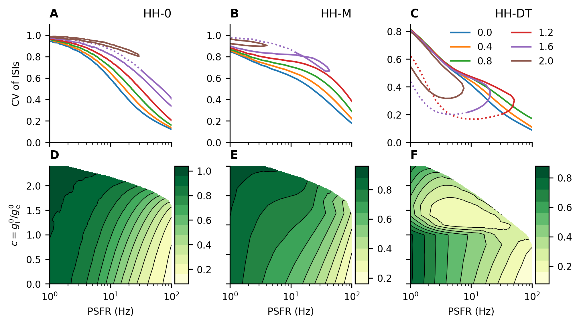
Figure 4: The effect of membrane potential stabilization on spiking regularity in the Hodgkin-Huxley models. A-C: Dependence of the $\mathrm{C}_{\mathrm{V}}$ of ISIs on the firing rate for different values of $c$ (color-coded). The dotted parts of the curves represent the sections where $\lambda_{\mathrm{e}}>$100\text{\,}\mathrm{kHz}$$. In the subthreshold regimes, the output rate reaches its maximum and then starts dropping to zero. For the HH-DT model (C), the $\mathrm{C}_{\mathrm{V}}$ decreases at this point, whereas for the HH-0 (A) and HH-M (B) models, no clear improvement is observed. D-F: Contour plots with color-coded $\mathrm{C}_{\mathrm{V}}$, $c$ on the $y$-axis. If more than one input can produce the same PSFR with the same $c$, the lowest possible value of $\mathrm{C}_{\mathrm{V}}$ is color-coded. Note that there is no discontinuity in F, unlike in Fig. 3F. The transition to the more regular states with growing $c$ is continuous, as is illustrated in Supplementary Figure 4. The data points were obtained from simulations with different input intensities $\lambda_{\mathrm{e}}$, $\lambda_{\mathrm{i}}$.

Increasing $c$ in the HH-DT subthreshold regime decreases the $\mathrm{C}_{\mathrm{V}}$. However, it is important to note that increased $c$ does not imply stronger inhibitory input in this case. In fact, increasing the inhibitory input rate $\lambda_{\mathrm{i}}$ is almost always beneficial for the spike-firing regularity in the HH-DT model, and this is also the case in the DT-LIF model (Fig 5). From this, we conclude that if a neuron exhibits a dynamic threshold, a stimulus will produce a more regular spike train if it elicits an increase in inhibitory input simultaneously with excitatory input.

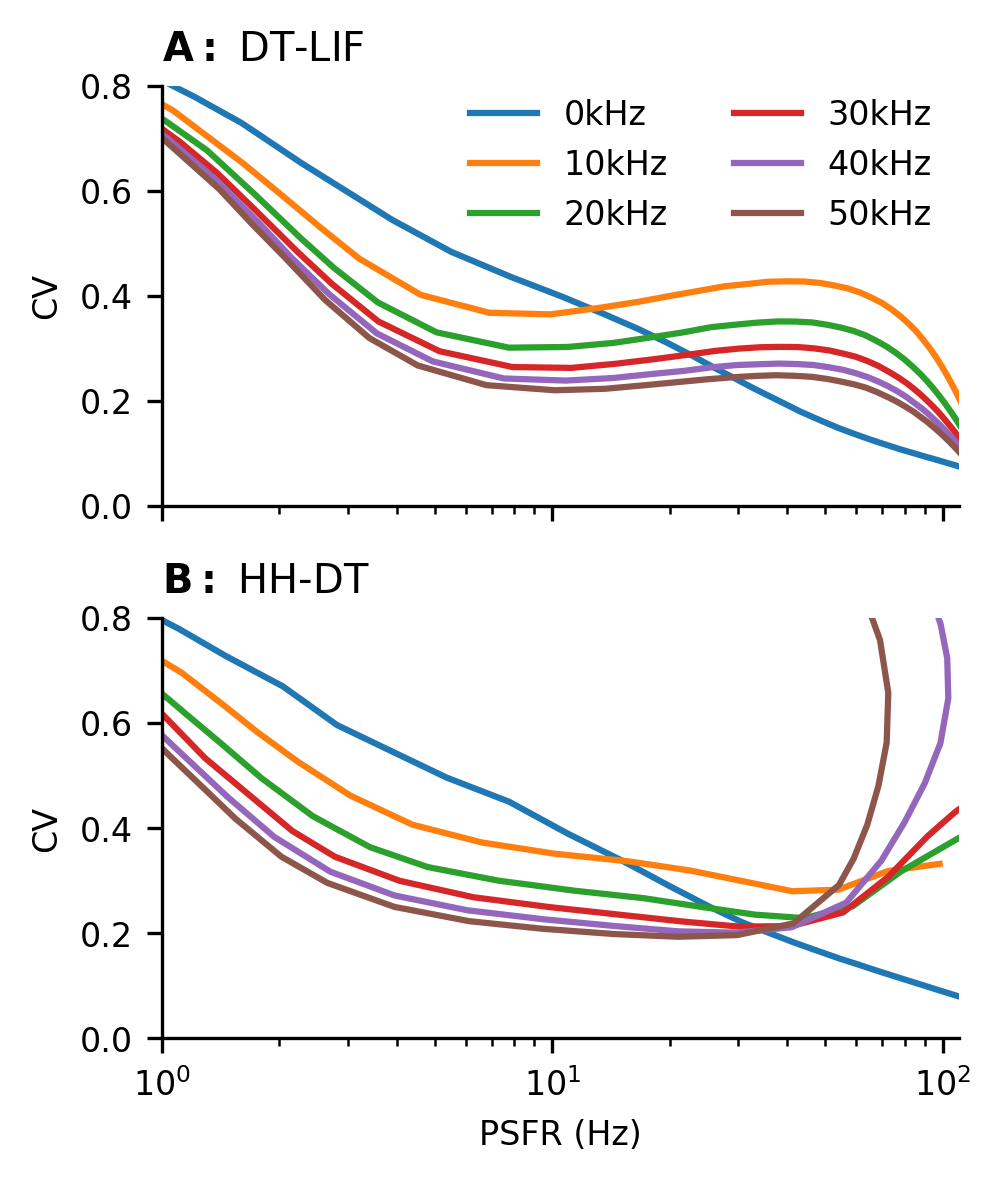
Figure 5: Constant inhibition trajectories for the dynamic threshold models. In both the DT-LIF (A) and HH-DT (B) models, increasing the pre-synaptic inhibitory firing rate (color) is beneficial for the firing regularity (measured by $\mathrm{C}_{\mathrm{V}}$, $y$-axis) for a wide range of PSFRs ($x$-axis).

Discussion

Simplified input models

Absence of reversal potentials

If the reversal potentials are not taken into account, the synaptic currents are given by

$$I_{\mathrm{e},\mathrm{i}}(t)=\sum_{t_{k}\in\mathcal{T}_{\mathrm{e},\mathrm{i}}}H_{\mathrm{e},\mathrm{i}}(t-t_{k}),$$ (37)

where $H$ is again a filtering function. If the two currents are uncorrelated, they will add up to an input current with mean value $I_{0}$ and standard deviation $\sigma_{I}$. If the diffusion approximation is employed (the current is modeled as an Ornstein-Uhlenbeck process with a time constant $\tau_{I}$), the mean and standard deviation of the membrane potential are [63]:

$$\langle V\rangle_{I} =E_{\mathrm{L}}+\frac{I_{0}}{g_{\mathrm{L}}},$$ (38)

$$\sigma_{V,I}^{2} =\sigma_{I}^{2}\frac{\tau_{I}}{a^{2}g_{\mathrm{L}}(C+g_{\mathrm{L}}\tau_{I})}.$$ (39)

In the absence of synaptic reversal potentials, the variance diverges with growing input, and increasing the synaptic current fluctuations by increasing $\lambda_{\mathrm{e}}$ and $\lambda_{\mathrm{i}}$ clearly increases the membrane potential fluctuations, in contrast to the model with synaptic reversal potential.

Absence of synaptic filtering

If synaptic filtering is neglected, $h_{\mathrm{e},\mathrm{i}}$ become $\delta$-functions:

$$h_{\mathrm{e},\mathrm{i}}(t)=Ca_{\mathrm{e},\mathrm{i}}\delta(t),$$ (40)

where $C$ is the membrane capacitance, and $a_{\mathrm{e},\mathrm{i}}$ governs the jump in the membrane potential $\Delta V$ triggered by a single pulse:

$$\Delta V=(E_{\mathrm{e},\mathrm{i}}-V)(1-e^{-a_{\mathrm{e},\mathrm{i}}}).$$ (41)

This model was studied extensively, e.g., in [32, 23, 31]. In [23, 31], the formulas for the mean membrane potential and its standard deviation are calculated in the diffusion approximation:

$$\langle V\rangle_{W} =\tau(E_{\mathrm{L}}\tau_{L}^{-1}+E_{\mathrm{e}}\lambda_{\mathrm{e}}b_{\mathrm{e}}+E_{\mathrm{i}}\lambda_{\mathrm{i}}b_{\mathrm{i}})$$ (42)

$$\sigma_{V,W}^{2} =\frac{\tau_{L}}{2}\frac{\lambda_{\mathrm{e}}b_{\mathrm{e}}^{2}(\langle V\rangle-E_{\mathrm{e}})^{2}+\lambda_{\mathrm{i}}b_{\mathrm{i}}^{2}(\langle V\rangle-E_{\mathrm{i}})^{2}}{1+\tau_{L}\lambda_{\mathrm{e}}b_{\mathrm{e}}(1-b_{\mathrm{e}}/2)+\tau_{L}\lambda_{\mathrm{i}}b_{\mathrm{i}}(1-b_{\mathrm{i}}/2)},$$ (43)

where

$$\tau^{-1} =\tau_{L}^{-1}+\lambda_{\mathrm{e}}b_{\mathrm{e}}+\lambda_{\mathrm{i}}b_{\mathrm{i}}$$ (44)

$$b_{\mathrm{e},\mathrm{i}} =1-e^{-a_{\mathrm{e},\mathrm{i}}}.$$ (45)

Richardson [23] reported that a higher inhibition-to-excitation ratio may lead to a decrease in the membrane potential fluctuations for strongly hyperpolarized membranes. However, the effect of inhibition reverses as the membrane potential depolarizes (Fig 6). Furthermore, the membrane potential does not stabilize within the limit of infinite firing rates. Therefore, the time correlation of synaptic input introduced by synaptic filtering is necessary to observe the shunting effect of inhibitory synapses.

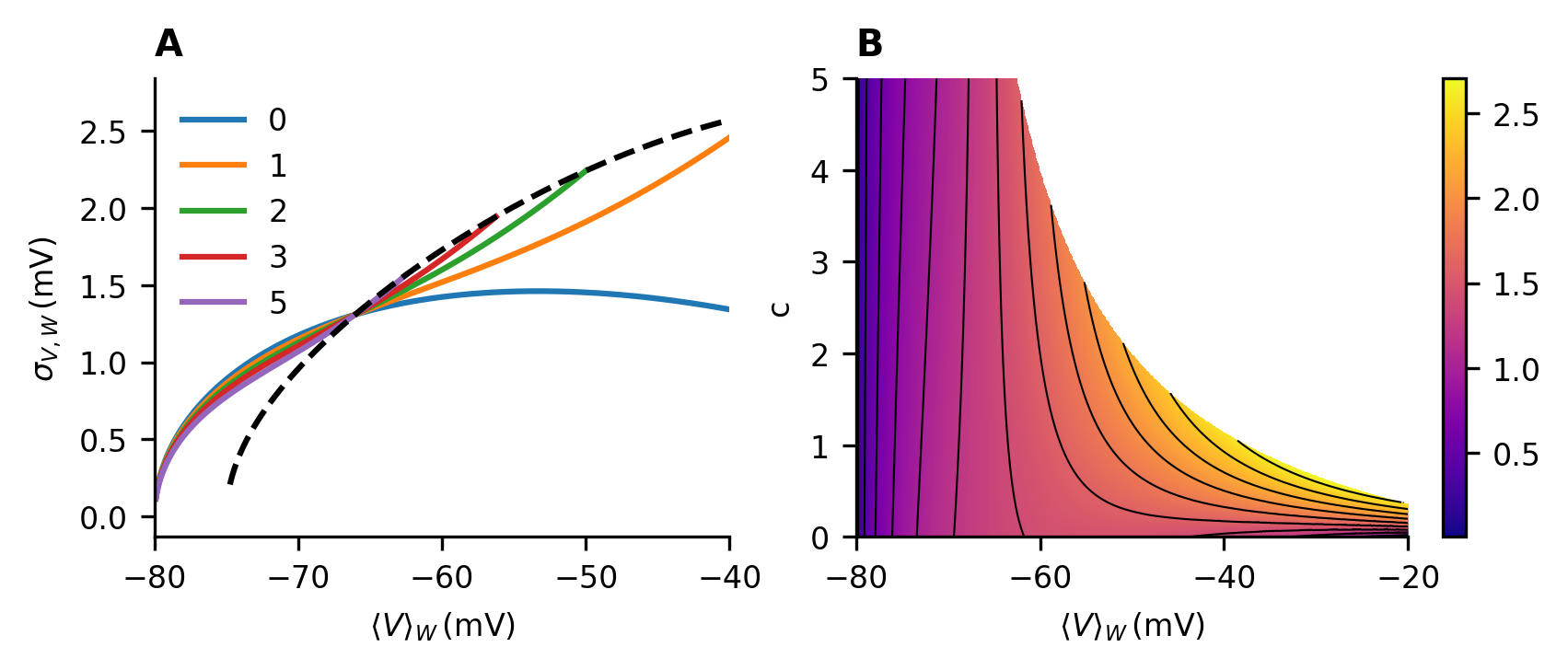
Figure 6: Membrane potential with conductance input without synaptic filtering. A: Membrane potential fluctuations as a function of the mean membrane potential for different values of $c=\frac{\lambda_{\mathrm{i}}b_{\mathrm{i}}}{\lambda_{\mathrm{e}}b_{\mathrm{e}}}$ (color-coded), as calculated from the Eqs (42,43). The dashed line represents the limit $\lim\limits_{\lambda_{\mathrm{e}},\lambda_{\mathrm{i}}\rightarrow\infty}\sigma_{V,W}(\langle V\rangle_{W})$. The membrane potential is not stabilized at infinite inputs. Above certain depolarizations, inhibition increases membrane potential fluctuations, contrary to the case of conductance input with synaptic filtering. B: Heatmap with color-coded standard deviation of the membrane potential. Parameters used were $b_{\mathrm{e}}=0.0045$, $b_{\mathrm{i}}=0.0150$.

Regular firing in multicompartmental models

The models analyzed in this work are all single-compartmental models, i.e., models in which the charge is distributed infinitely fast across the cell, and the membrane potential is therefore the same everywhere. In reality, neurons receive input predominantly at dendrites, and the spikes are initiated in the soma. To account for this fact, multicompartmental models are typically employed. The soma and dendritic parts can be modeled as two separate compartments (for simplicity, as two identical cylinders) connected through a coupling conductance $g_{c}$ :

$$C\frac{\mathrm{d}V_{S}}{\mathrm{d}t} =-g_{\mathrm{L}}(V_{S}-E_{\mathrm{L}})-g_{c}(V_{S}-V_{D})$$ (46)

$$\begin{split}C\frac{\mathrm{d}V_{D}}{\mathrm{d}t}&=-g_{\mathrm{L}}(V_{D}-E_{\mathrm{L}})-g_{c}(V_{D}-V_{S})-\\ &-\frac{1}{a_{D}}(g_{\mathrm{e}}(V_{D}-E_{\mathrm{e}})+g_{\mathrm{i}}(V_{D}-E_{\mathrm{i}}))\end{split}$$ (47)

where $V_{S}$ and $V_{D}$ are the membrane potentials of the somatic and dendritic compartments, respectively; $a_{D}$ is the dendritic area; and $V_{S}$ is reset to $V_{r}$ when the threshold $\theta$ is reached.

In the hypothetical case of infinite input rates, $V_{D}=V_{\infty}(c)$ and $V_{S}$ periodically decay to $V_{S}^{0}=\frac{g_{\mathrm{L}}E_{\mathrm{L}}+g_{c}V_{D}}{g_{\mathrm{L}}+g_{c}}$ with a time constant $\tau_{2}=\frac{g_{\mathrm{L}}+g_{c}}{a_{S}C}$, resulting in regular ISIs

$$T=-\tau_{2}\log\left(1+\frac{V_{r}-\theta}{V_{S}^{0}-V_{r}}\right).$$ (48)

Therefore, it is possible to reach a wide range of firing rates with $\mathrm{C}_{\mathrm{V}}{}=0$ and decrease $\mathrm{C}_{\mathrm{V}}$ while maintaining a constant mean firing rate by increasing $c$, similar to the case of LIF with a dynamic threshold.

The coupling conductance can be calculated as $g_{c}=\frac{d}{4R_{a}l^{2}}$ [64], where $d$ is the diameter of the cylinder, $l$ is the length, and $R_{a}=$150\text{\,}\mathrm{\SIUnitSymbolOhm}\text{\,}\mathrm{cm}$$ is the longitudinal resistance. If we consider that the original area of the neuron approximately $3.5\text{\times}{10}^{-4}\text{\,}\mathrm{c}\mathrm{m}^{2}$ is split between the two cylinders and we set $d=l$, we obtain $\tau_{2}\approx$4.5\text{\,}\mathrm{\SIUnitSymbolMicro s}$$. It is therefore unlikely that firing rate regularization with biologically relevant post-synaptic firing rates would be observed with biologically plausible inputs.

Conclusion

We demonstrate that a higher inhibition-to-excitation ratio and subsequently higher synaptic current fluctuations lead to a more stable membrane potential if the stimulation is modeled as time-filtered activation of synaptic conductances with reversal potentials. Our analysis thus provides a theoretical context for the experimental observations of [19]. Moreover, our results highlight the importance of incorporating synaptic filtering and reversal potentials into neuronal simulations. The qualitative differences between neurons stimulated with white noise and colored noise current have been reported in the literature [26, 27, 28]. However, we demonstrate that realistic synaptic filtering with reversal potentials is responsible for a novel fluctuation-stabilization mechanism which cannot be observed in simplified models.

We analyzed the impact of membrane potential stabilization on spike-firing regularity in GLIF models and HH-type models. We compared the effects of an increased inhibition-to-excitation ratio on two different mechanisms of spike-firing adaptation: adaptation by a hyperpolarizing ionic current (AHP and M-current adaptation) and adaptation implemented as a dynamic firing threshold. Both SFA mechanisms are biologically relevant and are useful in neuronal modeling [47, 48, 65, 66, 42, 39, 67, 68]. We demonstrated that while an increase in inhibition leads to less regular spike trains in the ionic current adaptation models and models without any spike-firing adaptation, it may enhance the firing regularity in the dynamic threshold models. We observed this effect in both the GLIF models and HH-type models.

High presynaptic inhibitory activity is typical of cortical neurons. In the so called high-conductance state, total inhibitory conductance can be several-fold larger than total excitatory conductance [11]. Our findings therefore provide a novel view of the importance of the high-conductance state and inhibitory synapses in biological neural networks.

Appendix A Effective time constant approximation

The Eqs (1,2) can be rewritten as:

$$Ca\frac{\mathrm{d}V}{\mathrm{d}t}=-g_{0}(V-E_{0})-g_{\mathrm{e}}^{F}(V-E_{\mathrm{e}})-g_{\mathrm{i}}^{F}(V-E_{\mathrm{i}}),$$ (49)

where $g_{0}=ag_{\mathrm{L}}+g_{\mathrm{e}}^{0}+g_{\mathrm{i}}^{0}$, $g_{\mathrm{e},\mathrm{i}}^{0}$, and $g_{\mathrm{e},\mathrm{i}}^{F}$ are the mean and fluctuating parts of the conductance input. The input can then be separated into its additive and multiplicative parts:

$$g_{\mathrm{e}}^{F}(V-E_{\mathrm{e}})=g_{\mathrm{e}}^{F}(E_{0}-E_{\mathrm{e}})+g_{\mathrm{e}}^{F}(V-E_{0}).$$ (50)

By neglecting the multiplicative part $g_{\mathrm{e}}^{F}(V-E_{0})$, we obtain the effective time constant approximation (ETA). In the diffusion approximation, the mean and standard deviation of the membrane potential are [23, 24]:

$$\langle V\rangle_{\mathrm{ETA}} =E_{0},$$ (51)

$$\begin{split}\sigma_{V,\mathrm{ETA}}^{2}&=\left(\frac{\sigma_{\mathrm{e}}}{g_{0}}\right)^{2}(E_{\mathrm{e}}-E_{0})\frac{\tau_{\mathrm{e}}}{\tau_{\mathrm{e}}+\tau_{0}}+\\ &+\left(\frac{\sigma_{\mathrm{i}}}{g_{0}}\right)^{2}(E_{\mathrm{i}}-E_{0})\frac{\tau_{\mathrm{i}}}{\tau_{\mathrm{i}}+\tau_{0}},\end{split}$$ (52)

where $\tau_{0}=\frac{aC}{g_{0}}$ is the effective time constant, and $\sigma_{\mathrm{e},\mathrm{i}}$ are the standard deviations of the excitatory and inhibitory inputs.

Appendix B Limit cases of LIF and AHP-LIF models

High conductance limit of the LIF model

If $V_{\infty}(c)>\theta$, in the case of high input intensities, $V_{\mathrm{ef}}$ is permanently above the threshold, and the effective membrane time constant $\tau(g_{\mathrm{e}},g_{\mathrm{i}})$ approaches zero. Therefore, in the absence of a refractory period, the firing rate $f=\frac{1}{\mu_{\mathrm{ISI}}}$ diverges ($\mu_{\mathrm{ISI}}$ is the average ISI). If the average postsynaptic ISI is much shorter than synaptic timescales, we can assume that the input remains effectively constant during the entire ISI (corresponding to the adiabatic approximation [28, 69, 70, 71, 72]). The length of the ISI is then determined solely by the immediate values of the excitatory and inhibitory conductances

$$T(g_{\mathrm{e}},g_{\mathrm{i}})=-\frac{aC}{ag_{\mathrm{L}}+g_{\mathrm{e}}+g_{\mathrm{i}}}\log\left(\frac{\theta-V_{\mathrm{ef}}(g_{\mathrm{e}},g_{\mathrm{i}})}{V_{r}-V_{\mathrm{ef}}(g_{\mathrm{e}},g_{\mathrm{i}})}\right).$$ (53)

Assuming independence of the inputs, the mean ISI and its standard deviation can then be approximated as

$$\mu_{\mathrm{ISI}}=-\frac{aC}{g_{\mathrm{tot}}}\log\left(\frac{\theta-E_{0}}{V_{r}-E_{0}}\right),$$ (54)

$$\sigma_{\mathrm{ISI}}^{2}=\left(\frac{\partial T}{\partial g_{\mathrm{e}}}\right)^{2}\Bigr{|}_{\begin{subarray}{c}g_{\mathrm{e}}=g_{\mathrm{e}}^{0}\end{subarray}}\sigma_{\mathrm{e}}^{2}+\left(\frac{\partial T}{\partial g_{\mathrm{i}}}\right)^{2}\Bigr{|}_{\begin{subarray}{c}g_{\mathrm{i}}=g_{\mathrm{i}}^{0}\end{subarray}}\sigma_{\mathrm{i}}^{2}=$$ (55)

$$=(aC)^{2}g_{\mathrm{e}}^{0}\left[\frac{A_{\mathrm{e}}\left((E_{\mathrm{e}}-E_{0})(\theta-V_{r})+\alpha\right)}{g_{\mathrm{tot}}^{4}(\theta-E_{0})^{2}(E_{0}-V_{r})^{2}}\right.+$$

$$+\left.\frac{cA_{\mathrm{i}}\left((E_{\mathrm{i}}-E_{0})(\theta-V_{r})+\alpha\right)}{g_{\mathrm{tot}}^{4}(\theta-E_{0})^{2}(E_{0}-V_{r})^{2}}\right],$$

$$\alpha=(\theta-E_{0})(E_{0}-V_{r})\log\frac{E_{0}-\theta}{E_{0}-V_{r}},$$

where $g_{\mathrm{tot}}=ag_{\mathrm{L}}+g_{\mathrm{e}}^{0}+g_{\mathrm{i}}^{0}$ (for validity of the approximation see Fig. 7). Therefore, $\sigma_{\mathrm{ISI}}/\mu_{\mathrm{ISI}}=O\left(\left(g_{\mathrm{e}}^{0}\right)^{-1/2}\right)$. We conclude that with growing input intensity, the firing rate diverges and $\mathrm{C}_{\mathrm{V}}{}\rightarrow 0$.

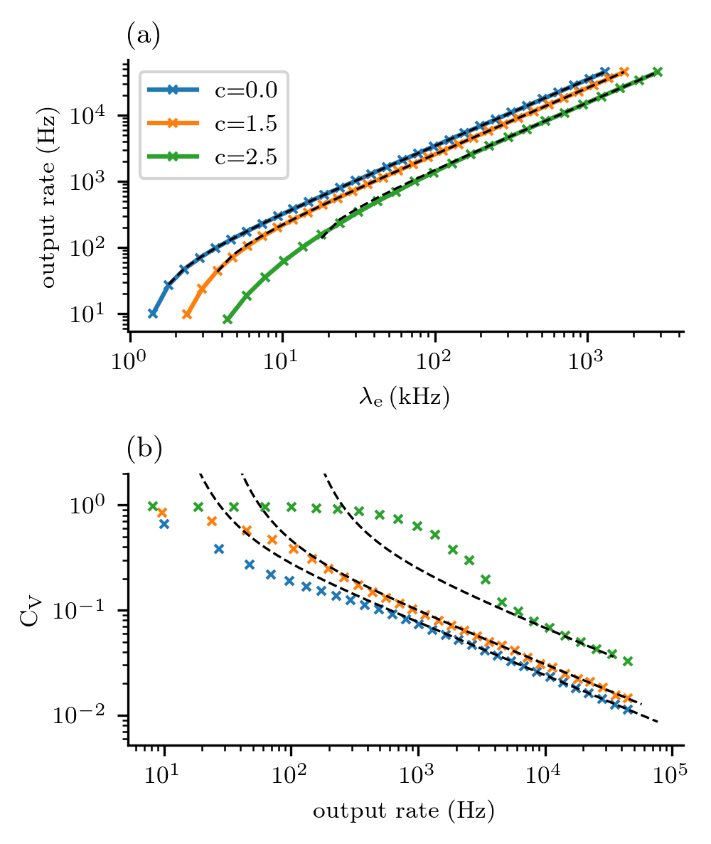
Figure 7: Approximation of the PSFR and $\mathrm{C}_{\mathrm{V}}$ of LIF. Simulation results are color-coded. The dashed lines represent the approximations from the Eqs (54,55). The firing rate is approximated very well (A). $\mathrm{C}_{\mathrm{V}}$ is approximated well for very high PSFRs ($>$1\text{\,}\mathrm{kHz}$$) (B). This is due to the short input time constants ($3\text{\,}\mathrm{ms}$ for excitatory, $10\text{\,}\mathrm{ms}$ for inhibitory). For the simulation, we used the timestep $\Delta t=$0.1\text{\,}\mathrm{ms}$$ if the expected PSFR was $<$100\text{\,}\mathrm{Hz}$$ and $\Delta t\frac{\mu_{\mathrm{ISI}}}{$10\text{\,}\mathrm{ms}$}$ otherwise.

High conductance limit of the AHP-LIF model

Effective reversal potential

We follow the assumption that the fluctuations in $V_{\mathrm{ef}}(g_{\mathrm{e}},g_{\mathrm{i}})$ are very small and therefore $V_{\mathrm{ef}}^{\mathrm{AHP}}$ (Eq. (7)) is permanently above the threshold $\theta$. With the ISI $\mu_{\mathrm{ISI}}^{\mathrm{AHP}}\ll\tau_{\mathrm{AHP}}$, $g_{\mathrm{AHP}}(t)\approx\langle g_{\mathrm{AHP}}(t)\rangle=\frac{\Delta g\tau_{\mathrm{AHP}}}{\mu_{\mathrm{ISI}}^{\mathrm{AHP}}}$. Analogously to the Eq. (54)), we can use the following implicit equation to approximate the mean ISI:

$$\mu_{\mathrm{ISI}}^{\mathrm{AHP}}=-\frac{aC}{g_{\mathrm{tot}}^{\mathrm{AHP}}}\log\frac{\theta-E_{0}^{\mathrm{AHP}}}{V_{r}-E_{0}^{\mathrm{AHP}}},,$$ (56)

where

$$g_{\mathrm{tot}}^{\mathrm{AHP}} =ag_{\mathrm{L}}+g_{\mathrm{e}}^{0}+g_{\mathrm{i}}^{0}+\frac{\Delta g\tau_{\mathrm{AHP}}}{\mu_{\mathrm{ISI}}^{\mathrm{AHP}}},$$ (57)

$$E_{0}^{\mathrm{AHP}} =\frac{ag_{\mathrm{L}}E_{\mathrm{L}}+g_{\mathrm{e}}^{0}E_{\mathrm{e}}+g_{\mathrm{i}}^{0}E_{\mathrm{i}}+\frac{\Delta g\tau_{\mathrm{AHP}}}{\mu_{\mathrm{ISI}}^{\mathrm{AHP}}}E_{\mathrm{K}}}{g_{\mathrm{tot}}^{\mathrm{AHP}}}.$$ (58)

We continue to evaluate the high-conductance limit of $E_{0}^{\mathrm{AHP}}$:

$$\begin{gathered}\lim\limits_{g_{\mathrm{e}}^{0}\rightarrow+\infty}E_{0}^{\mathrm{AHP}}=V_{\infty}^{\mathrm{AHP}}(c)\equiv\\ \equiv\lim\limits_{g_{\mathrm{e}}^{0}\rightarrow+\infty}\frac{\frac{ag_{\mathrm{L}}}{g_{\mathrm{e}}^{0}}E_{\mathrm{L}}+E_{\mathrm{e}}+cE_{\mathrm{i}}+\frac{\tau_{\mathrm{AHP}}}{g_{\mathrm{e}}^{0}\mu_{\mathrm{ISI}}^{\mathrm{AHP}}}\Delta gE_{\mathrm{K}}}{\frac{ag_{\mathrm{L}}}{g_{\mathrm{e}}^{0}}+1+c+\frac{\tau_{\mathrm{AHP}}}{g_{\mathrm{e}}^{0}\mu_{\mathrm{ISI}}^{\mathrm{AHP}}}\Delta g}.\end{gathered}$$ (59)

Clearly, $\frac{ag_{\mathrm{L}}}{g_{\mathrm{e}}^{0}}\rightarrow 0$. Therefore, it is important to evaluate the limit $A=\lim\limits_{g_{\mathrm{e}}^{0}\rightarrow+\infty}g_{\mathrm{e}}^{0}\mu_{\mathrm{ISI}}^{\mathrm{AHP}}$. Then:

$$V_{\infty}^{\mathrm{AHP}}(c)=\frac{E_{\mathrm{e}}+cE_{\mathrm{i}}+\frac{\tau_{\mathrm{AHP}}}{A}\Delta gE_{\mathrm{K}}}{1+c+\frac{\tau_{\mathrm{AHP}}}{A}\Delta g}.$$ (60)

By multiplying both sides of Eq. ((56)) with $g_{\mathrm{tot}}^{\mathrm{AHP}}$ and then taking the limit of both sides of the equation, we obtain:

$$ag_{\mathrm{L}}\mu_{\mathrm{ISI}}+g_{\mathrm{e}}^{0}(1+c)\mu_{\mathrm{ISI}}+\tau_{\mathrm{AHP}}\Delta g=-aC\log\frac{\theta-V_{\infty}^{\mathrm{AHP}}}{V_{r}-V_{\infty}^{\mathrm{AHP}}},$$ (61)

$$A(1+c)+\tau_{\mathrm{AHP}}\Delta g=-aC\log\frac{\theta-V_{\infty}^{\mathrm{AHP}}}{V_{r}-V_{\infty}^{\mathrm{AHP}}}.$$ (62)

Numerical solution of Eq. ((62)) allows us to compare $V_{\infty}^{\mathrm{AHP}}(c)$ with $V_{\infty}(c)$ and thus provides a comparison between the LIF model with and without the M-current adaptation (Fig. 8). For approximately $c>5$ (with the used parameters), $V_{\infty}(c)^{\mathrm{AHP}}\approx\theta$. Therefore, the neuron requires a very high input intensity for the fluctuations to be so small that $V_{\mathrm{ef}}^{\mathrm{AHP}}$ permanently exceeds the threshold, and in the range of biologically feasible inputs, the fluctuations in $V_{\mathrm{ef}}^{\mathrm{AHP}}$ lead to bursting when $V_{\mathrm{ef}}^{\mathrm{AHP}}>\theta$ and are silent when $V_{\mathrm{ef}}^{\mathrm{AHP}}\leq\theta$ (Fig. 8).

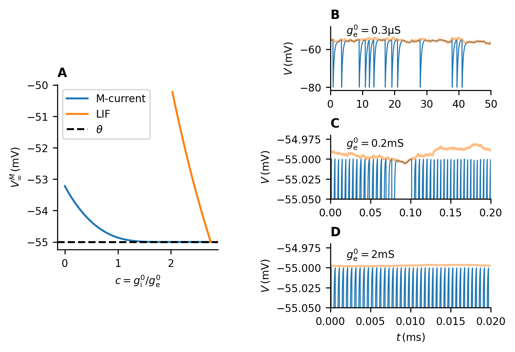
Figure 8: High conductance limit of the AHP-LIF model A: Equilibrium potential (in mV) in the infinite conductance limit (Eq. (60)) for different values of $c$ (shown in blue). For high $c$, the value $V_{\infty}^{\mathrm{AHP}}(c)$ is very close to the threshold (dashed black line). The value of $V_{\infty}(c)$ (33), corresponding to the LIF model, is shown in orange for comparison. The M-current adaptation clearly pushes the equilibrium potential closer to the threshold, leading to bursting behavior. B-D: Time-course of the membrane potential of LIF with M-current adaptation with $c=1.7$ for different values of input intensities. The membrane potential (shown in blue) follows closely $V_{\mathrm{ef}}^{\mathrm{AHP}}$ (shown in orange). When $V_{\mathrm{ef}}^{\mathrm{AHP}}>\theta$, the neuron is bursting; otherwise, the neuron is silent. With higher input intensities, the probability of $V_{\mathrm{ef}}^{\mathrm{AHP}}\leq\theta$ drops, and the firing rate becomes increasingly more regular.

The limit of $\mathrm{C}_{\mathrm{V}}$

Neglecting the variance of $g_{\mathrm{AHP}}(t)$, the variance of ISIs can then be approximated analogously to Eq. ((55)) as:

$$\sigma_{\mathrm{ISI}}^{2}=\left(\frac{\partial\mu_{\mathrm{ISI}}}{\partial g_{\mathrm{e}}}\right)^{2}\sigma_{\mathrm{e}}^{2}+\left(\frac{\partial\mu_{\mathrm{ISI}}}{\partial g_{\mathrm{i}}}\right)^{2}\sigma_{\mathrm{i}}^{2},$$ (63)

Our goal is to demonstrate that the coefficient of variation ($\mathrm{C}_{\mathrm{V}}$) approaches zero. Using the definition of $\mathrm{C}_{\mathrm{V}}$ (Eq. (26)) and Eq. (56), we have

$$\lim\limits_{g_{\mathrm{e}}^{0}\rightarrow+\infty}\mathrm{C}_{\mathrm{V}}{}=\lim\limits_{g_{\mathrm{e}}^{0}\rightarrow+\infty}\frac{\sigma_{\mathrm{ISI}}}{\mu_{\mathrm{ISI}}}$$ (64)

$$=-\lim\limits_{g_{\mathrm{e}}^{0}\rightarrow+\infty}\frac{g_{\mathrm{tot}}^{\mathrm{AHP}}}{aC}\frac{\sigma_{\mathrm{ISI}}}{\log\frac{\theta-E_{0}^{\mathrm{AHP}}}{V_{r}-E_{0}^{\mathrm{AHP}}}}$$ (65)

$$=-\lim\limits_{g_{\mathrm{e}}^{0}\rightarrow+\infty}g_{\mathrm{tot}}^{\mathrm{AHP}}\sigma_{\mathrm{ISI}}\lim\limits_{g_{\mathrm{e}}^{0}\rightarrow+\infty}\left(\log\frac{\theta-E_{0}^{\mathrm{AHP}}}{V_{r}-E_{0}^{\mathrm{AHP}}}\right)^{-1}.$$ (66)

Since $-\infty<\lim\limits_{g_{\mathrm{e}}^{0}\rightarrow+\infty}\left(\log\frac{\theta-E_{0}^{\mathrm{AHP}}}{V_{r}-E_{0}^{\mathrm{AHP}}}\right)^{-1}<0$, it remains to be shown that $\lim\limits_{g_{\mathrm{e}}^{0}\rightarrow+\infty}g_{\mathrm{tot}}^{\mathrm{AHP}}\sigma_{\mathrm{ISI}}=0$, which can be shown by using the implicit differentiation formula.

See pages 1 of supplementary_figures.pdf See pages 0 of supplementary_figures.pdf

References

- Matsumura et al. [1988] M. Matsumura, T. Cope, and E. Fetz, Sustained excitatory synaptic input to motor cortex neurons in awake animals revealed by intracellular recording of membrane potentials, Exp. Brain Res. 70, 463–469 (1988).
- Rudolph et al. [2007] M. Rudolph, M. Pospischil, I. Timofeev, and A. Destexhe, Inhibition Determines Membrane Potential Dynamics and Controls Action Potential Generation in Awake and Sleeping Cat Cortex, J. Neurosci. 27, 5280 (2007).
- Steriade et al. [2001] M. Steriade, I. Timofeev, and F. Grenier, Natural Waking and Sleep States: A View From Inside Neocortical Neurons, J. Neurophysiol. 85, 1969 (2001).
- Shadlen and Newsome [1994] M. N. Shadlen and W. T. Newsome, Noise, neural codes and cortical organization, Curr. Opin. Neurobiol. 4, 569 (1994).
- Vreeswijk and Sompolinsky [1996] C. v. Vreeswijk and H. Sompolinsky, Chaos in Neuronal Networks with Balanced Excitatory and Inhibitory Activity, Science 274, 1724 (1996).
- Shadlen and Newsome [1998] M. N. Shadlen and W. T. Newsome, The Variable Discharge of Cortical Neurons: Implications for Connectivity, Computation, and Information Coding, J. Neurosci. 18, 3870 (1998).
- Amit and Brunel [1997] D. Amit and N. Brunel, Model of global spontaneous activity and local structured activity during delay periods in the cerebral cortex, Cereb. Cortex 7, 237 (1997).
- Brunel [2000] N. Brunel, Dynamics of Sparsely Connected Networks of Excitatory and Inhibitory Spiking Neurons, J. Comput. Neurosci. 8, 183 (2000).
- Destexhe [2010] Destexhe, Inhibitory “noise”, Front Cell Neurosci Front. Cell. Neurosci. 4, (2010).
- Denève and Machens [2016] S. Denève and C. K. Machens, Efficient codes and balanced networks, Nat. Neurosci 19, 375 (2016).
- Destexhe et al. [2003] A. Destexhe, M. Rudolph, and D. Paré, The high-conductance state of neocortical neurons in vivo, Nat. Rev. Neurosci. 4, 739 (2003).
- Bernander et al. [1991] O. Bernander, R. J. Douglas, K. A. Martin, and C. Koch, Synaptic background activity influences spatiotemporal integration in single pyramidal cells., Proc. Natl. Acad. Sci. U.S.A. 88, 11569 (1991).
- Paré et al. [1998] D. Paré, E. Shink, H. Gaudreau, A. Destexhe, and E. J. Lang, Impact of Spontaneous Synaptic Activity on the Resting Properties of Cat Neocortical Pyramidal Neurons In Vivo, J. Neurophysiol. 79, 1450 (1998).
- Mittmann et al. [2005] W. Mittmann, U. Koch, and M. Häusser, Feed-forward inhibition shapes the spike output of cerebellar Purkinje cells, J. Physiol. 563, 369 (2005).
- Wolfart et al. [2005] J. Wolfart, D. Debay, G. L. Masson, A. Destexhe, and T. Bal, Synaptic background activity controls spike transfer from thalamus to cortex, Nat. Neurosci. 8, 1760 (2005).
- Sengupta et al. [2013] B. Sengupta, S. B. Laughlin, and J. E. Niven, Balanced Excitatory and Inhibitory Synaptic Currents Promote Efficient Coding and Metabolic Efficiency, PLoS Comput. Biol. 9, e1003263 (2013).
- D’Onofrio et al. [2019] G. D’Onofrio, P. Lansky, and M. Tamborrino, Inhibition enhances the coherence in the Jacobi neuronal model, Chaos Solitons Fractals 128, 108 (2019).
- Barta and Kostal [2019] T. Barta and L. Kostal, The effect of inhibition on rate code efficiency indicators, PLoS Comput Biol. 15, e1007545 (2019).
- Monier et al. [2003] C. Monier, F. Chavane, P. Baudot, L. J. Graham, and Y. Frégnac, Orientation and Direction Selectivity of Synaptic Inputs in Visual Cortical Neurons, Neuron 37, 663 (2003).
- Churchland et al. [2010] M. M. Churchland, B. M. Yu, J. P. Cunningham, L. P. Sugrue, M. R. Cohen, G. S. Corrado, W. T. Newsome, A. M. Clark, P. Hosseini, B. B. Scott, D. C. Bradley, M. A. Smith, A. Kohn, J. A. Movshon, K. M. Armstrong, T. Moore, S. W. Chang, L. H. Snyder, S. G. Lisberger, N. J. Priebe, I. M. Finn, D. Ferster, S. I. Ryu, G. Santhanam, M. Sahani, and K. V. Shenoy, Stimulus onset quenches neural variability: a widespread cortical phenomenon., Nat. Neurosci 13, 369 (2010).
- Fatt and Katz [1953] P. Fatt and B. Katz, The effect of inhibitory nerve impulses on a crustacean muscle fibre, J. Physiol. 121, 374 (1953).
- Wolff and Lindner [2010] L. Wolff and B. Lindner, Mean, Variance, and Autocorrelation of Subthreshold Potential Fluctuations Driven by Filtered Conductance Shot Noise, Neural Comput. 22, 94 (2010).
- Richardson [2004] M. J. E. Richardson, Effects of synaptic conductance on the voltage distribution and firing rate of spiking neurons, Phys Rev E 69, 051918 (2004).
- Richardson and Gerstner [2005] M. J. E. Richardson and W. Gerstner, Synaptic Shot Noise and Conductance Fluctuations Affect the Membrane Voltage with Equal Significance, Neural Comput. 17, 923 (2005).
- Lindner and Schimansky-Geier [2001] B. Lindner and L. Schimansky-Geier, Transmission of Noise Coded versus Additive Signals through a Neuronal Ensemble, Phys. Rev. Lett. 86, 2934 (2001).
- Brunel et al. [2001] N. Brunel, F. S. Chance, N. Fourcaud, and L. F. Abbott, Effects of Synaptic Noise and Filtering on the Frequency Response of Spiking Neurons, Phys. Rev. Lett. 86, 2186 (2001).
- Fourcaud and Brunel [2002] N. Fourcaud and N. Brunel, Dynamics of the Firing Probability of Noisy Integrate-and-Fire Neurons, Neural Comput. 14, 2057 (2002).
- Moreno-Bote and Parga [2004] R. Moreno-Bote and N. Parga, Role of Synaptic Filtering on the Firing Response of Simple Model Neurons, Phys. Rev. Lett. 92, 028102 (2004).
- Schwalger and Schimansky-Geier [2008] T. Schwalger and L. Schimansky-Geier, Interspike interval statistics of a leaky integrate-and-fire neuron driven by Gaussian noise with large correlation times, Phys Rev E 77, 031914 (2008).
- Droste and Lindner [2017] F. Droste and B. Lindner, Exact analytical results for integrate-and-fire neurons driven by excitatory shot noise, J. Comput. Neurosci 43, 81 (2017).
- Richardson and Gerstner [2006] M. J. E. Richardson and W. Gerstner, Statistics of subthreshold neuronal voltage fluctuations due to conductance-based synaptic shot noise, Chaos 16, 26106 (2006).
- Lánská et al. [1994] V. Lánská, P. Lánský, and C. E. Smith, Synaptic Transmission in a Diffusion Model for Neural Activity, J. Theor. Biol. 166, 393 (1994).
- Deger et al. [2012] M. Deger, M. Helias, C. Boucsein, and S. Rotter, Statistical properties of superimposed stationary spike trains, J. Comput. Neurosci 32, 443 (2012).
- Sanzeni et al. [2020] A. Sanzeni, M. H. Histed, and N. Brunel, Response nonlinearities in networks of spiking neurons, PLoS Comput. Biol. 16, e1008165 (2020).
- Martinez [2005] D. Martinez, Oscillatory Synchronization Requires Precise and Balanced Feedback Inhibition in a Model of the Insect Antennal Lobe, Neural Comput. 17, 2548 (2005).
- Peron and Gabbiani [2009] S. P. Peron and F. Gabbiani, Role of spike-frequency adaptation in shaping neuronal response to dynamic stimuli, Biol. Cybern. 100, 505 (2009).
- Augustin et al. [2013] M. Augustin, J. Ladenbauer, and K. Obermayer, How adaptation shapes spike rate oscillations in recurrent neuronal networks, Front. Comput. Neurosci. 7, (2013).
- Ha and Cheong [2017] G. E. Ha and E. Cheong, Spike Frequency Adaptation in Neurons of the Central Nervous System, Exp. Neurobiol 26, 179 (2017).
- Levakova et al. [2019] M. Levakova, L. Kostal, C. Monsempès, P. Lucas, and R. Kobayashi, Adaptive integrate-and-fire model reproduces the dynamics of olfactory receptor neuron responses in a moth, J R Soc Interface 16, 20190246 (2019).
- Betkiewicz et al. [2020] R. Betkiewicz, B. Lindner, and M. P. Nawrot, Circuit and Cellular Mechanisms Facilitate the Transformation from Dense to Sparse Coding in the Insect Olfactory System, eNeuro 7, 0305 (2020).
- Benda and Herz [2003] J. Benda and A. V. M. Herz, A Universal Model for Spike-Frequency Adaptation, Neural Comput. 15, 2523 (2003).
- Kobayashi and Kitano [2016] R. Kobayashi and K. Kitano, Impact of slow K+ currents on spike generation can be described by an adaptive threshold model, J. Comput. Neurosci. 40, 347 (2016).
- Tuckwell [1988] H. C. Tuckwell, Introduction to Theoretical Neurobiology (Cambridge University Press, 1988).
- Dayan and Abbott [2005] P. Dayan and L. F. Abbott, Theoretical Neuroscience: Computational and Mathematical Modeling of Neural Systems (The MIT Press, 2005).
- Destexhe et al. [2001] A. Destexhe, M. Rudolph, J. M. Fellous, and T. J. Sejnowski, Fluctuating synaptic conductances recreate in vivo-like activity in neocortical neurons., Neuroscience 107, 13 (2001).
- Gerstner et al. [2019] W. Gerstner, W. M. Kistler, and R. Naud, Neuronal Dynamics (Cambridge University Press, 2019).
- Teeter et al. [2018] C. Teeter, R. Iyer, V. Menon, N. Gouwens, D. Feng, J. Berg, A. Szafer, N. Cain, H. Zeng, M. Hawrylycz, C. Koch, and S. Mihalas, Generalized leaky integrate-and-fire models classify multiple neuron types, Nat. Commun 9, 709 (2018).
- Benda et al. [2010] J. Benda, L. Maler, and A. Longtin, Linear Versus Nonlinear Signal Transmission in Neuron Models With Adaptation Currents or Dynamic Thresholds, J. Neurophysiol 104, 2806 (2010).
- Destexhe and Paré [1999] A. Destexhe and D. Paré, Impact of Network Activity on the Integrative Properties of Neocortical Pyramidal Neurons In Vivo, J. Neurophysiol 81, 1531 (1999).
- Softky and Koch [1993] W. R. Softky and C. Koch, The highly irregular firing of cortical cells is inconsistent with temporal integration of random EPSPs, J. Neurosci 13, 334 (1993).
- Heyman and Sobel [2004] D. P. Heyman and M. J. Sobel, Stochastic Models in Operations Research: Stochastic Processes and Operating Characteristics, Dover Books on Computer Science Series (Dover Publications, 2004).
- Lindner [2006] B. Lindner, Superposition of many independent spike trains is generally not a Poisson process, Phys Rev E 73, 022901 (2006).
- Kingman [1993] J. F. C. Kingman, Poisson Processes (Oxford Studies in Probability) (Clarendon Press, 1993).
- Amit and Tsodyks [1992] D. J. Amit and M. V. Tsodyks, Effective neurons and attractor neural networks in cortical environment, Network 3, 121 (1992).
- Toyoizumi et al. [2006] T. Toyoizumi, K. Aihara, and S.-i. Amari, Fisher Information for Spike-Based Population Decoding, Phys. Rev. Lett. 97, 098102 (2006).
- Kostal et al. [2007] L. Kostal, P. Lansky, and J.-P. Rospars, Neuronal coding and spiking randomness, Eur. J. Neurosci 26, 2693 (2007).
- de Ruyter van Steveninck [1997] R. R. de Ruyter van Steveninck, Reproducibility and Variability in Neural Spike Trains, Science 275, 1805 (1997).
- Strong et al. [1998] S. P. Strong, R. Koberle, R. R. de Ruyter van Steveninck, and W. Bialek, Entropy and Information in Neural Spike Trains, Phys. Rev. Lett. 80, 197 (1998).
- Tiesinga et al. [2000] P. H. E. Tiesinga, J. V. José, and T. J. Sejnowski, Comparison of current-driven and conductance-driven neocortical model neurons with Hodgkin-Huxley voltage-gated channels, Phys Rev E 62, 8413 (2000).
- Chacron et al. [2004] M. J. Chacron, B. Lindner, and A. Longtin, Noise Shaping by Interval Correlations Increases Information Transfer, Phys. Rev. Lett. 92, 080601 (2004).
- Lindner et al. [2005] B. Lindner, M. J. Chacron, and A. Longtin, Integrate-and-fire neurons with threshold noise: A tractable model of how interspike interval correlations affect neuronal signal transmission, Phys Rev E 72, 021911 (2005).
- Farkhooi et al. [2011] F. Farkhooi, E. Muller, and M. P. Nawrot, Adaptation reduces variability of the neuronal population code, Phys Rev E 83, 050905 (2011).
- Lindner and Longtin [2006] B. Lindner and A. Longtin, Comment on “Characterization of Subthreshold Voltage Fluctuations in Neuronal Membranes,” by M. Rudolph and A. Destexhe, Neural Comput. 18, 1896 (2006).
- Sterratt et al. [2011] D. Sterratt, B. Graham, A. Gillies, and D. Willshaw, Principles of Computational Modelling in Neuroscience (Cambridge University Press, 2011).
- Chacron et al. [2000] M. J. Chacron, A. Longtin, M. St-Hilaire, and L. Maler, Suprathreshold Stochastic Firing Dynamics with Memory in P-Type Electroreceptors, Phys. Rev. Lett. 85, 1576 (2000).
- Kobayashi et al. [2009] R. Kobayashi, Y. Tsubo, and S. Shinomoto, Made-to-order spiking neuron model equipped with a multi-timescale adaptive threshold, Front. Comput. Neurosci. 3, 9 (2009).
- Gerstner and Naud [2009] W. Gerstner and R. Naud, How Good Are Neuron Models?, Science 326, 379 (2009).
- Kobayashi et al. [2019] R. Kobayashi, S. Kurita, A. Kurth, K. Kitano, K. Mizuseki, M. Diesmann, B. J. Richmond, and S. Shinomoto, Reconstructing neuronal circuitry from parallel spike trains, Nat. Commun. 10, 4468 (2019).
- Moreno-Bote and Parga [2005] R. Moreno-Bote and N. Parga, Membrane Potential and Response Properties of Populations of Cortical Neurons in the High Conductance State, Phys. Rev. Lett. 94, 088103 (2005).
- Moreno-Bote and Parga [2006] R. Moreno-Bote and N. Parga, Auto- and Crosscorrelograms for the Spike Response of Leaky Integrate-and-Fire Neurons with Slow Synapses, Phys. Rev. Lett. 96, 028101 (2006).
- Moreno-Bote et al. [2008] R. Moreno-Bote, A. Renart, and N. Parga, Theory of Input Spike Auto- and Cross-Correlations and Their Effect on the Response of Spiking Neurons, Neural Comput. 20, 1651 (2008).
- Moreno-Bote and Parga [2010] R. Moreno-Bote and N. Parga, Response of Integrate-and-Fire Neurons to Noisy Inputs Filtered by Synapses with Arbitrary Timescales: Firing Rate and Correlations, Neural Comput. 22, 1528 (2010).