SISSA 05/2021/FISI

FTUV-21-0119.3119

IFIC/21-02

Modular Invariant Dynamics
and Fermion Mass Hierarchies around $\tau=i$
Ferruccio Feruglio¹ , Valerio Gherardi² , Andrea Romanino^2,3  and Arsenii Titov^1,4 

¹Dipartimento di Fisica e Astronomia ‘G. Galilei’, Università di Padova
INFN, Sezione di Padova, Via Marzolo 8, I-35131 Padua, Italy
²SISSA, International School for Advanced Studies,
INFN, Sezione di Trieste, Via Bonomea 265, I-34136 Trieste, Italy
³ICTP, Strada Costiera 11, I-34151 Trieste, Italy
⁴Departament de Física Teòrica, Universitat de València
IFIC, Universitat de València-CSIC, Dr. Moliner 50, E-46100 Burjassot, Spain

We discuss fermion mass hierarchies within modular invariant flavour models. We analyse the neighbourhood of the self-dual point $\tau=i$, where modular invariant theories possess a residual $Z_{4}$ invariance. In this region the breaking of $Z_{4}$ can be fully described by the spurion $\epsilon\approx\tau-i$, that flips its sign under $Z_{4}$. Degeneracies or vanishing eigenvalues of fermion mass matrices, forced by the $Z_{4}$ symmetry at $\tau=i$, are removed by slightly deviating from the self-dual point. Relevant mass ratios are controlled by powers of $|\epsilon|$. We present examples where this mechanism is a key ingredient to successfully implement an hierarchical spectrum in the lepton sector, even in the presence of a non-minimal Kähler potential.

1 Introduction

Revealing the origin(s) of fermion masses and explaining the structure of quark and lepton mixing are among the deepest long-standing questions in particle physics. Looking for an organising principle behind the observed patterns of fermion masses and mixing, flavour symmetries have been proposed and extensively studied in the last several decades (see ref. [1] for a recent review). In spite of a significant theoretical effort resulting in many models able to describe certain pieces of the flavour puzzle, there is arguably no fundamental theory of flavour. Still, the concept of symmetry is admittedly among the best tools we have to search for such a theory.

While in the pure bottom-up approach flavour symmetries are introduced as a new ingredient, in the top-down perspective they may arise from a UV completion of the Standard Model (SM), perhaps string theory. Today a theory of flavour fully derived from string theory represents a formidable unsolved problem, due to the huge number of possible solutions, and we might be led to consider a more modest approach where the large freedom related to a bottom-up procedure is mitigated by some guiding principle. In particular, in ref. [2], modular invariance arising in many string compactifications has been proposed as a candidate for flavour symmetry in the lepton sector.

In the simplest case, modular invariance arises from the compactification of a higher dimensional theory on a torus or an orbifold. Size and shape of the compact space are parametrised by a modulus $\tau$ living in the upper-half complex plane, up to modular transformations. These can be interpreted as discrete gauge transformations, related to the redundancy of the description. The low-energy effective theory, relevant to the known particle species, has to obey modular invariance and Yukawa couplings become functions of $\tau$. The framework has a big conceptual advantage. In a generic bottom-up approach, realistic flavour symmetries require an ad-hoc symmetry breaking sector, with Vacuum Expectation Values (VEVs) of scalar multiplets — the flavons — carefully tailored in size and orientation. In minimal schemes based on modular invariance, flavons are not needed and the scalar sector can be completely replaced by the moduli space. Moreover the action of modular invariance in generation space occurs through a well-defined set of finite groups. Continuous groups and many discrete groups are not allowed, thus reducing the arbitrariness of the construction.

The proposal has been accompanied by several significant developments and activity in model building (for a review, see [1] and references therein). Recently, the proposed framework of modular invariant supersymmetric theories of flavour has been extended to incorporate (in a non-trivial way) several moduli [3]. The latter might be needed to describe different sectors of a theory, i.e. quarks, charged leptons and neutrinos. Moreover, the role of modular invariance as flavour symmetry has been intensively investigated in the last two years from a top-down perspective [4, 5, 6, 7], resulting, in particular, in the concept of eclectic flavour symmetries [8, 9, 10, 11, 12]. A top-down construction incorporating several moduli has been very recently formulated in refs. [13, 14].

Despite the appealing aspects, realistic realisations of the framework have still to face several difficulties. In the vast majority of phenomenologically viable modular invariant models constructed so far, the observed hierarchies, in particular those between the charged lepton masses, are achieved by tuning free parameters entering the superpotential. Moreover, even if the requirement of modular invariance represents a severe constraint at the level of the Yukawa couplings of the (supersymmetric) theory, it allows in general a much larger freedom at the level of kinetic terms [2, 15]. Non-minimal kinetic terms are allowed, with corresponding free parameters that affect the prediction of fermion masses and mixing angles. Finally, so far the modulus is mainly treated as a free parameter, varied to optimise the agreement with the data. In concrete models, the preferred value of $\tau$ often occurs in the vicinity of the self-dual point $\tau=i$ (see, e.g. refs. [2, 16, 17, 18, 19, 20, 21, 22, 23, 24, 25, 26]), where one of the generators of the modular group remains unbroken. In CP invariant realisations, it has been realised that CP violation can be explained by a small departure of the modulus from this special point, where CP is unbroken [2, 19]. It remains to be understood how the dynamics drives the modulus in the vicinity of, but not exactly on, the self-dual point.

In this article, we aim to address the question of whether the lepton mass hierarchies can originate from modular invariance alone, with the Lagrangian parameters being $\mathcal{O}(1)$ quantities. Some attempts to explain mass hierarchies avoiding fine tuning have been made in refs. [27, 28]. In the former study, new fields singlet under both the SM gauge group and finite modular group, but carrying non-trivial modular weights, have been introduced, whereas in the latter work expansions of modular forms around fixed points $\tau=i$, $\tau=\omega\equiv e^{2\pi i/3}$ and $\tau=i\infty$ have been employed, and a semi-analytic study of the fermion mass matrices has been performed . We go beyond previous works discussing in detail the structure of the modular invariant theory near $\tau=i$, which is motivated by phenomenological models.

At this point, the theory has a residual $Z_{4}$ symmetry (cf. ref. [24]). We show that the action of this symmetry can be realised linearly, even when $\tau\neq i$. In particular, $\epsilon\approx\tau-i$ behaves as a (small) spurion with $Z_{4}$ charge $+2$. Thus, in a vicinity of $\tau=i$, we have a $Z_{4}$ symmetric theory broken by $\epsilon$. Similar considerations apply to other fixed points as well. We show that the residual $Z_{4}$ symmetry can be exploited to reduce the rank of the charged lepton mass matrix at $\tau=i$, with small non-vanishing masses arising from a small departure from the self-dual point.

As we will see in explicit models, when a minimal Kähler potential is adopted, the constraints coming from modular invariance realised near $\tau=i$ can be too restrictive to allow full agreement with the experimental data. We are thus led to discuss non-minimal candidates of Kähler potential, their pattern around $\tau=i$ and their impact on the predictions for masses, mixing angles and CP-violating (CPV) phases. The presence of extra inputs related to a more general Kähler potential is expected to reduce the predictability of our setup. Nevertheless, our analysis suggests that the arbitrariness coming from the Kähler potential can be partially tamed precisely by mass matrices of reduced rank. Moreover, in the models discussed in this paper, a non-minimal Kähler potential allows to obtain full agreement with the data, without being the dominant source of the observed hierarchies. Further constraints on the Kähler potential and consequent improvement in predictability could come by extending the modular group to an eclectic flavour symmetry, where modular invariance is enhanced by a traditional finite flavour symmetry [9].

The article is organised as follows. In Section 2, we review the formalism of supersymmetric modular invariant flavour theories. Next, in Section 3, we zoom in on their structure near $\tau=i$ and discuss linear realisation of the associated residual $Z_{4}$ symmetry. Further, in Section 4, we present examples of modular invariant models at level 3 where flavour hierarchies are generated by a small departure from $\tau=i$. Finally, we draw our conclusions in Section 5. Appendix A discusses the most general form of the Kähler potential quadratic in the modular forms of level 3 and weight 2.

2 Modular invariant models

In this section we shortly review the formalism of supersymmetric modular invariant theories [34, 35] applied to flavour physics [2]. The theory depends on a set of chiral supermultiplets $\varphi$ comprising the dimensionless modulus $\tau\equiv\varphi_{0}/\Lambda$ (${\tt Im}~{}\tau>0$) and other superfields $\varphi_{i}$ $(i\geq 1)$. Here $\Lambda$ represents the cut-off of our effective theory, and can be interpreted as the relevant mass scale of an underlying fundamental theory. In the case of rigid supersymmetry, the Lagrangian $\mathscr{L}$  is fully specified by the Kähler potential $K(\varphi,\bar{\varphi})$, a real gauge-invariant function of the chiral multiplets and their conjugates, by the superpotential $W(\varphi)$, a holomorphic gauge-invariant function of the chiral multiplets, and by the gauge kinetic function $f(\varphi)$, a dimensionless holomorphic gauge-invariant function of the chiral superfields. Neglecting gauge interactions, we have:

$$\mathscr{L}=\int d^{2}\theta d^{2}\bar{\theta}~{}K(\varphi,\bar{\varphi})+\int d^{2}\theta~{}W(\varphi)+\int d^{2}\bar{\theta}~{}{\overline{W}}(\bar{\varphi})~{}~{}~{}.$$ (1)

The Lagrangian is invariant under transformations $\gamma$ of the homogeneous modular group $\Gamma=SL(2,Z)$:

$$\tau\to\gamma\tau=\frac{a\tau+b}{c\tau+d}~{}~{}~{},~{}~{}~{}~{}~{}\varphi_{i}\to(c\tau+d)^{-k_{i}}\rho(\tilde{\gamma})_{ij}\varphi_{j}~{}~{}~{}~{}(i,j\geq 1)~{}~{}~{},$$ (2)

where $a$, $b$, $c$, $d$ are integers obeying $ad-bc=1$. Such transformations are generated by the two elements of $\Gamma$:

$$S=\begin{pmatrix}0&1\\ -1&0\end{pmatrix}\qquad\text{and}\qquad T=\begin{pmatrix}1&1\\ 0&1\end{pmatrix}~{}~{}.$$ (3)

The matrix $\rho(\tilde{\gamma})$ is a unitary representation of the group $\Gamma_{N}=\Gamma/\Gamma(N)$, obtained as a quotient between the group $\Gamma$ and a principal congruence subgroup $\Gamma(N)$, the positive integer $N$ being the level of the representation. The level $N$ is kept fixed in the construction, and $\tilde{\gamma}$ represents the equivalence class of $\gamma$ in $\Gamma_{N}$. In general $\rho(\tilde{\gamma})$ is a reducible representation and all superfields belonging to the same irreducible component should have the same weight $k_{i}$, here assumed to be integer  . In the following, we denote by $(\varphi_{i},\psi_{i})$ the spin-$(0,1/2)$ components of the chiral superfields $\varphi_{i}$ $(i\geq 1)$ . The terms bilinear in the fermion fields read [37]:

$$\mathscr{L}_{F}=\mathscr{L}_{F,K}+\mathscr{L}_{F,2}\,,$$ (4)

with :

$$\mathscr{L}_{F,K}=i\,K^{j}_{i}\,\overline{\psi}_{j}\bar{\sigma}^{\mu}D_{\mu}\psi^{i}~{},~{}~{}~{}~{}~{}\mathscr{L}_{F,2}=-\frac{1}{2}\left[W_{ij}-W_{l}(K^{-1})^{l}_{m}K^{m}_{ij}\right]\psi^{i}\psi^{j}+\text{h.c.}~{},$$ (5)

where lower (upper) indices in $K$ and $W$ stand for derivatives with respect to holomorphic (anti-holomorphic) fields. When the scalar fields in eq. (5) take their VEVs, we can move to the basis where matter fields are canonically normalised, through a transformation:

$$\psi^{i}\to(z^{-1/2})_{ij}\psi^{j}~{}~{}~{},$$ (6)

where the matrix $(z^{1/2})_{ij}$ satisfies: $K^{j}_{i}=[(z^{1/2})^{\dagger}]^{jl}(z^{1/2})_{li}$ . We can identify the fermion mass matrix as:

$$m_{kn}=\left[W_{ij}-W_{l}(K^{-1})^{l}_{m}K^{m}_{ij}\right](z^{-1/2})_{ik}(z^{-1/2})_{jn}~{}~{}~{},$$ (7)

where VEVs are understood. In the previous equation, the second term in the square bracket vanishes when supersymmetry is unbroken and the VEV of $W_{l}$ is zero. When we turn on supersymmetry breaking effects, the first term is expected to dominate over the second one, provided there is a sufficient gap between the sfermion masses $m_{\mathrm{SUSY}}$ and the messenger/cutoff scale $M$. This holds both for vector-like and for chiral fermions. Indeed, up to loop factors or other accidental factors, the VEVs of $W_{l}$, $W_{ij}$ and $K^{m}_{ij}$ are of the order of $m_{\mathrm{SUSY}}M$, $M$ and $1/M$, respectively, when fermions are vector-like. When chiral fermions are considered, $W_{ij}$ and $K^{m}_{ij}$ are both depleted by $v/M$ with respect to the vector-like case, $v$ denoting the gauge symmetry breaking scale. Thus we have a relative suppression between the two contributions of order $m_{\mathrm{SUSY}}/M$, which can be made tiny (cf. ref. [17]). If we work under this assumption, the mass matrix is well approximated by:

$$m_{kn}=W_{ij}~{}(z^{-1/2})_{ik}(z^{-1/2})_{jn}~{}~{}~{}.$$ (8)

The supersymmetry breaking terms neglected here can be useful to give masses to light fermions, which otherwise would remain massless in the exact supersymmetry limit. We will come back to this point when discussing concrete models, in Section 4. Due to the conservation of the electric charge, the equality of eq. (8) holds separately in any charge sector. By focusing on the lepton sector $(E^{c},L)$ and by assuming that the neutrino masses arise from the Weinberg operator, we have:

$$W=-E^{c}_{i}\,\mathcal{Y}^{e}_{ij}(\tau)L_{j}H_{d}-\frac{1}{2\Lambda_{L}}L_{i}\,\mathcal{C}^{\nu}_{ij}(\tau)L_{j}H_{u}H_{u}~{}~{}~{},$$ (9)

where $H_{u,d}$ are the Higgs chiral multiplets and $\Lambda_{L}$ is the scale where lepton number is broken. The general relation (8) specialises into:

$$m_{e}=(z^{-1/2}_{E^{c}})^{T}{\mathcal{Y}}^{e}(\tau)(z^{-1/2}_{L})~{}v_{d}~{}~{}~{},~{}~{}~{}~{}~{}~{}m_{\nu}=(z^{-1/2}_{L})^{T}{\mathcal{C}}^{\nu}(\tau)(z^{-1/2}_{L})~{}v_{u}^{2}/\Lambda_{L}~{}~{}~{},$$ (10)

where we have absorbed the renormalisation factors for $H_{u,d}$ in the definition of their VEVs. In Section 4, we will also comment on the special limit where $z^{-1/2}_{E^{c},L}$ are universal, i.e. proportional to the unit matrix. The mass matrices obtained in this case will be referred to as “bare” matrices and denoted by $m_{e,\nu}^{(0)}$. An important consequence of modular invariance is the special functional dependence of ${\mathcal{Y}}^{e}(\tau)$ and ${\mathcal{C}}^{\nu}(\tau)$ on the modulus $\tau$. Under a transformation of $\Gamma$, the chiral multiplets $(E^{c}_{i},L_{i},H_{u,d})$ transform as in eq. (2), with weights $(k_{E^{c}_{i}},k_{L_{i}},k_{H_{u,d}})$ and representations $(\rho_{E^{c}}(\tilde{\gamma}),\rho_{L}(\tilde{\gamma}),\mathbb{1})$. For the superpotential $W$ to be modular invariant, ${\mathcal{Y}}^{e}(\tau)$ and ${\mathcal{C}}^{\nu}(\tau)$ should obey:

$${\mathcal{Y}}^{e}(\gamma\tau)=(c\tau+d)^{{k_{e}}}~{}\rho_{E^{c}}^{*}(\tilde{\gamma})~{}{\mathcal{Y}}^{e}(\tau)\rho_{L}^{\dagger}(\tilde{\gamma})~{},~{}~{}~{}~{}~{}{\mathcal{C}}^{\nu}(\gamma\tau)=(c\tau+d)^{{k_{\nu}}}~{}\rho_{L}^{*}(\tilde{\gamma})~{}{\mathcal{C}}^{\nu}(\tau)\rho_{L}^{\dagger}(\tilde{\gamma})~{},$$ (11)

where the weights $k_{e,\nu}$ are matrices satisfying: $(k_{e})_{ij}=k_{E^{c}_{i}}+k_{L_{j}}+k_{H_{d}}$ and $(k_{\nu})_{ij}={k_{L}}_{i}+{k_{L}}_{j}+2k_{H_{u}}$. Thus ${\mathcal{Y}}^{e}(\tau)$ and ${\mathcal{C}}^{\nu}(\tau)$ are modular forms of given level and weight. Since the linear space of such modular forms is finite dimensional, the choices for ${\mathcal{Y}}^{e}(\tau)$ and ${\mathcal{C}}^{\nu}(\tau)$ are limited. If neutrino masses originate from a type I seesaw mechanism, eqs. (9) and (10) hold with the identification:

$$\frac{{\mathcal{C}}^{\nu}(\tau)}{\Lambda_{L}}=-({\mathcal{Y}}^{\nu}(\tau))^{T}~{}{\mathcal{M}}(\tau)^{-1}~{}{\mathcal{Y}}^{\nu}(\tau)~{}~{}~{},$$ (12)

where ${\mathcal{Y}}^{\nu}(\tau)$ and ${\mathcal{M}}(\tau)$ denote the matrix of neutrino Yukawa couplings and the mass matrix of the heavy electroweak singlets $N^{c}$, respectively. Notice that there is no dependence on the renormalisation factor $(z^{-1/2}_{N^{c}})$ of the heavy modes. In some cases ${\mathcal{Y}}^{e}(\tau)$ and/or ${\mathcal{C}}^{\nu}(\tau)$ are completely determined as a function of $\tau$ up to an overall constant, thus providing a strong potential constraint on the mass spectrum, eq. (10).

Unfortunately, such property does not extend to the Kähler potential $K$ and to the renormalisation factors $(z^{-1/2}_{E^{c},L})$. Minimal choices of $K$, appropriate for a perturbative regime, can receive large non-perturbative corrections in the region of the moduli space we will consider. Without a control over the non-perturbative dynamics, in a generic point of the moduli space the factors $(z^{-1/2}_{E^{c},L})$ remain unknown. If we allowed for completely arbitrary $(z^{-1/2}_{E^{c},L})$, under mild conditions any mass matrix could be predicted. From eq. (10) we see that, given ${\mathcal{Y}}^{e}(\tau)$ and $(z^{-1/2}_{L})$, we could reproduce any desired matrix $m_{e}$, by selecting a particular $(z^{-1/2}_{E^{c}})^{T}$:

$$(z^{-1/2}_{E^{c}})^{T}=m_{e}~{}({\mathcal{Y}}^{e}(\tau)v_{d}(z^{-1/2}_{L}))^{-1}~{}~{}~{}.$$ (13)

An arbitrary matrix $m_{e}$ would result in a completely unconstrained lepton mixing matrix. Similar considerations would apply to the neutrino mass matrix $m_{\nu}$.

The loss of predictability associated to the Kähler corrections may however be less severe than eq. (13) might suggest, for two reasons. First, note that the above solution requires a non-singular ${\mathcal{Y}}^{e}(\tau)$. A singular ${\mathcal{Y}}^{e}(\tau)$ can only give rise to a singular $m_{e}$. Correspondingly, a hierarchical ${\mathcal{Y}}^{e}(\tau)$ can only correspond to a hierarchical $m_{e}$, unless the eigenvalues of the matrix $(z^{-1/2}_{E^{c}})^{T}$ in eq. (13) come in very large ratios. Although we cannot exclude the latter possibility, here we focus on the class of models where the corrections associated to the Kähler potential do not alter the “bare” limit by more than about one order of magnitude. Hence a singular or nearly singular ${\mathcal{Y}}^{e}(\tau)$ will tame the loss of predictability associated with the Kähler potential. Needless to say, a hierarchical ${\mathcal{Y}}^{e}(\tau)$ is needed to reproduce the mass spectrum in the charged lepton sector. Different considerations apply to the neutrino sector, where a singular ${\mathcal{C}}^{\nu}(\tau)$ might not be a good first order approximation of the data.

A second constraint on the effect of the Kähler corrections arises in the vicinity of the fixed points of $\Gamma$, $\tau=i$, $\tau=-1/2+i\sqrt{3}/2$ and $\tau=i\infty$, invariant under the action of the elements $S$, $ST$ and $T$, respectively. In the following, we will assume the modulus to be in the vicinity of the point $\tau=i$, as suggested by several models to correctly reproduce the data. The invariance under $S$ provides a constraint on the possible form of the Kähler potential at $\tau=i$ and in its vicinity.

3 Residual symmetry near $\tau=i$

The residual symmetry of the theory at $\tau=i$ is the cyclic group $Z_{4}$ generated by the element $S$, whose action on the chiral multiplets $\varphi_{i}$ in $\tau=i$ can be read from eq. (2):

$$\varphi_{i}\to\sigma_{ij}\varphi_{j}~{}~{}~{},~{}~{}~{}~{}~{}~{}~{}~{}~{}~{}~{}~{}~{}~{}\sigma_{ij}=i^{k_{i}}\rho(\tilde{S})_{ij}~{}~{}~{}~{}(i,j>0)~{}~{}~{},$$ (14)

where $\sigma$ is unitary, $\sigma^{2}$ is a parity operator and $\sigma^{4}=\mathbb{1}$. To analyse the neighbourhood of $\tau=i$, we expand both the Kähler potential and the superpotential in powers of the matter fields $\varphi_{i}$ $(i>0)$ :

$$\begin{aligned} W&=\sum_{i_{1},...,i_{n}}Y_{i_{1},...,i_{n}}(\tau)~{}\varphi_{i_{1}}...\varphi_{i_{n}}+...\\ K&=\overline{\varphi}_{i}\,z^{i}_{~{}j}(\tau,\bar{\tau})\,\varphi_{j}+...\end{aligned}~{}~{}~{}.$$ (15)

In the vicinity of $\tau=i$, it is possible to cast the theory as an ordinary $Z_{4}$ invariant theory, where the symmetry acts linearly on the fields, slightly broken by the spurion $(\tau-i)$. When we depart from $\tau=i$, the $S$ elements acts on the fields as:

$$\tau\to-\frac{1}{\tau}~{}~{}~{},~{}~{}~{}~{}~{}~{}\varphi_{i}\to(-\tau)^{-k_{i}}\rho(\tilde{S})_{ij}\varphi_{j}~{}~{}~{}~{}(i,j>0)~{}~{}~{}.$$ (16)

We perform the field redefinition:

$$\begin{cases}\displaystyle\tau=i\,\frac{i+\epsilon/2}{i-\epsilon/2}\\[8.5359pt] \displaystyle\tilde{\varphi}_{j}=\left(1-i\,\frac{\epsilon}{2}\right)^{-k_{j}}\varphi_{j}\end{cases}$$ (17)

mapping the upper-half complex plane into the disk $|\epsilon|<2$. In the linear approximation:

$$\epsilon=(\tau-i)+O\left((\tau-i)^{2}\right)~{}~{}~{}.$$ (18)

Under the $S$ transformation in (16), the new fields transform as:

$$\left\{\begin{aligned} &\epsilon\to-\epsilon\\[2.84526pt] &\tilde{\varphi}_{i}\to\sigma_{ij}~{}\tilde{\varphi}_{j}\end{aligned}\right.\;.$$ (19)

We see that the action of the $Z_{4}$ symmetry is linear in the new field basis, even when $\tau\neq i$. In particular $\epsilon$ behaves as a spurion with $Z_{4}$ charge $+2$. In the new field basis, the coefficients of the field expansion (15) read:

$$\begin{aligned} \tilde{Y}_{i_{1},\dots,i_{n}}&=\left(1-i\frac{\epsilon}{2}\right)^{k_{i_{1}}+\ldots+k_{i_{n}}}Y_{i_{1},\dots,i_{n}}\\ \tilde{z}^{i}_{~{}j}&=\left(1+i\frac{\bar{\epsilon}}{2}\right)^{k_{i}}z^{i}_{~{}j}\left(1-i\frac{\epsilon}{2}\right)^{k_{j}}\end{aligned}~{}~{}~{}.$$ (20)

The invariance of the theory under $Z_{4}$ requires $\tilde{Y}_{i_{1},...,i_{n}}(\epsilon)$ and $\tilde{z}^{i}_{~{}j}(\epsilon,\bar{\epsilon})$ to satisfy:

$$\begin{aligned} \tilde{Y}_{i_{1},...,i_{n}}(\epsilon)&=\sigma_{j_{1}i_{1}}~{}...~{}\sigma_{j_{n}i_{n}}\tilde{Y}_{j_{1},...,j_{n}}(-\epsilon)\\[5.69046pt] \tilde{z}^{i}_{~{}j}(\epsilon,\bar{\epsilon})&=\sigma^{\dagger ik}~{}\tilde{z}^{k}_{~{}l}(-\epsilon,-\bar{\epsilon})~{}\sigma_{lj}\end{aligned}~{}~{}~{}.$$ (21)

In particular, setting $\epsilon=0$, the above equations express the necessary conditions for the invariance of the theory at the symmetric point $\tau=i$. By expanding $\tilde{z}^{i}_{~{}j}(\epsilon,\bar{\epsilon})$ in powers of $\epsilon$ we see that the terms of first order vanish, up to possible non-diagonal terms relating fields with opposite value of $\sigma$. We conclude that in a neighbourhood of the fixed point $\tau=i$, and in the absence of any information about the Kähler potential, the theory reduces to a linearly realised $Z_{4}$ flavour symmetric theory, in the presence of a (small) spurion with charge $+2$.

4 Models

In this section, we present two models making use of the results of the previous section to account for the observed hierarchies in the lepton spectrum, namely the smallness of the charged lepton mass ratios, $m_{e}/m_{\tau}$ and $m_{\mu}/m_{\tau}$ and of the neutrino mass ratio $r\equiv\delta m^{2}/|\Delta m^{2}|$, where $\delta m^{2}\equiv m_{2}^{2}-m_{1}^{2}$ and $\Delta m^{2}\equiv m_{3}^{2}-(m_{1}^{2}+m_{2}^{2})/2$ (with the standard neutrino labelling). The hierarchies will be naturally accounted for by the small breaking of $Z_{4}$, $|\epsilon|\ll 1$, i.e. by the closeness of the modulus $\tau$ to the $Z_{4}$ symmetric point $\tau=i$, while the parameters in the superpotential will be $\mathcal{O}\left(1\right)$, and the corrections to the minimal Kähler will not be larger than $\mathcal{O}\left(1\right)$. In Table 1, we collect the best-fit values of the leptonic parameters with the corresponding $1\sigma$ uncertainties.

Observable	Best-fit value with $1\sigma$ error
$m_{e}/m_{\mu}$	$0.0048^{+0.0002}_{-0.0002}$
$m_{\mu}/m_{\tau}$	$0.0565^{+0.0045}_{-0.0045}$
	NO	IO
$\delta m^{2}\left[10^{-5}~{}\text{eV}^{2}\right]$	$7.42^{+0.21}_{-0.20}$
$\Delta m^{2}\left[10^{-3}~{}\text{eV}^{2}\right]$	$2.480^{+0.026}_{-0.028}$	$-2.461^{+0.028}_{-0.028}$
$r\equiv\delta m^{2}/|\Delta m^{2}|$	$0.0299^{+0.0009}_{-0.0009}$	$0.0301^{+0.0009}_{-0.0009}$
$\sin^{2}\theta_{12}$	$0.304^{+0.012}_{-0.012}$	$0.304^{+0.013}_{-0.012}$
$\sin^{2}\theta_{13}$	$0.02219^{+0.00062}_{-0.00063}$	$0.02238^{+0.00063}_{-0.00062}$
$\sin^{2}\theta_{23}$	$0.573^{+0.016}_{-0.020}$	$0.575^{+0.016}_{-0.019}$
$\delta/\pi$	$1.09^{+0.15}_{-0.13}$	$1.57^{+0.14}_{-0.17}$

Table 1: Best-fit values of the charged lepton mass ratios and the neutrino oscillation parameters with the corresponding 1$\sigma$ errors. For the charged lepton mass ratios we have used the values given in ref. [38], averaged over $\tan\beta$ as described in the text, whereas for the neutrino parameters we have used the results obtained in refs. [39, 40] (with Super-Kamiokande atmospheric data)

.

For the charged lepton mass ratios we use the results of ref. [38], where for $m_{\mu}/m_{\tau}$ we take an average between the values obtained for $\tan\beta=10$ and $\tan\beta=38$. For the neutrino oscillation parameters we employ the results of the global analysis performed in refs. [39, 40]. In what follows, when fitting models to the data, we use five dimensionless observables that have been measured with a good precision, i.e. two mass ratios , $m_{\mu}/m_{\tau}$ and $r$, and three leptonic mixing angles, $\sin^{2}\theta_{12}$, $\sin^{2}\theta_{13}$, $\sin^{2}\theta_{23}$. Regarding the Dirac CPV phase, $\delta$, values between $\pi$ and $2\pi$ (approximately) are currently allowed at $3\sigma$ for both neutrino mass spectrum with normal ordering (NO) and that with inverted ordering (IO). Moreover, in ref. [18], it has been shown that under the transformation $\tau\to-\tau^{\ast}$ and complex conjugation of couplings present in the superpotential, CPV phases change their signs, whereas masses and mixing angles remain the same. In fact, this reflects CP properties of modular invariant models [19] (see also [41]). As a consequence, the Dirac phase $\delta$ is not particularly constraining for our fits, and we do not include it in the list of input observables, regarding the obtained values as predictions.

4.1 Model 1: Weinberg operator and inverted ordering

We work at level 3, and the relevant finite modular group is $\Gamma_{3}$. In this subsection, we assume that neutrino masses are generated by the Weinberg operator. The field content of the model along with the assignment of $\Gamma_{3}$ representations and modular weights $k$ is shown in Table 2. The corresponding charges under $Z_{4}$, obtained using eq. (14), are shown in Table 3. We work in a real basis for the elements of $\Gamma_{3}$ where $\rho(\tilde{S})=\operatorname{\texttt{diag}}\,(+1,-1,-1)$ for the irreducible three-dimensional representation.

	$L$	$E_{1}^{c}$	$E_{2}^{c}$	$E_{3}^{c}$	$H_{u}$	$H_{d}$
$SU(2)_{L}\times U(1)_{Y}$	$(\mathbf{2},-1/2)$	$(\mathbf{1},+1)$	$(\mathbf{1},+1)$	$(\mathbf{1},+1)$	$(\mathbf{2},+1/2)$	$(\mathbf{2},-1/2)$
$\Gamma_{3}$	$\mathbf{3}$	$\mathbf{1}$	$\mathbf{1}$	$\mathbf{1^{\prime}}$	$\mathbf{1}$	$\mathbf{1}$
$k$	$1$	$3$	$3$	$3$	$0$	$0$

Table 2: Assignment of representations and modular weights in Model 1.

	$\tilde{L}_{1}$	$\tilde{L}_{2}$	$\tilde{L}_{3}$	$\tilde{E}_{1}^{c}$	$\tilde{E}_{2}^{c}$	$\tilde{E}_{3}^{c}$	$\tilde{H}_{u}$	$\tilde{H}_{d}$	$\epsilon$
$Z_{4}$	$1$	$-1$	$-1$	$-1$	$-1$	$-1$	$0$	$0$	2

Table 3: $Z_{4}$ charges (mod 4) in Model 1.

The quantum number assignments have immediate consequences for the charged lepton mass spectrum:

1. At $\tau=i$, the charged lepton mass matrix $m_{e}$ has rank one. This follows from the $Z_{4}$ charges in Table 3, forcing

   $$m_{e}=\begin{pmatrix}\alpha&0&0\\ \beta&0&0\\ \gamma&0&0\end{pmatrix}.$$ (22)

2. For a generic $\tau\neq i$, $m_{e}$ has rank two. While $Z_{4}$ alone would allow $m_{e}$ to have rank three, the underlying modular invariance forces the coefficients of the first and second rows of $m_{e}$ to be proportional, thus reducing the rank. In fact, modular invariance requires the coupling of $E_{1}^{c}$ and $E_{2}^{c}$ to $L$ to be proportional to the same modular form multiplet, namely, the triplet of weight four. The Kähler corrections cannot modify the rank condition. Thus, in the considered model, the electron has zero mass.

For $\tau\approx i+\epsilon$, with $\left|\epsilon\right|\ll 1$, we obtain the prediction

$$m_{e}\,\colon\,m_{\mu}\,\colon\,m_{\tau}=0\,\colon\,\mathcal{O}(\epsilon)\,\colon\,1\,.$$ (23)

Concerning the neutrino mass spectrum, from the charges of the lepton doublets $L_{i}$ in Table 3, we deduce that $m_{\nu}$ in $\tau=i$ takes the following general form:

$$m_{\nu}=\begin{pmatrix}0&a&b\\ a&0&0\\ b&0&0\end{pmatrix}.$$ (24)

This matrix has rank two and two degenerate non-zero eigenvalues. Notice that, while a generic $Z_{4}$ model would not account for the values of the parameters $a$ and $b$, here the underlying modular invariance fixes the relative values, before Kähler corrections. With the $Z_{4}$ assignment of Table 3, we are implicitly using the basis where $S$ is diagonal for the irreducible triplet of $\Gamma_{3}$ and we find $a/b=Y_{3}(i)/Y_{2}(i)$, where $Y^{(2)}(\tau)\equiv(Y_{1}(\tau),Y_{2}(\tau),Y_{3}(\tau))^{T}$ denotes the weight-two triplet of modular forms. On the other hand, generic Kähler corrections could mix $L_{2}$ and $L_{3}$, as they have the same $Z_{4}$ charge (see eq. (21)), leading to arbitrary $a/b$, as in generic $Z_{4}$ models. For $\tau\approx i+\epsilon$, the rank of $m_{\nu}$ becomes three, and we obtain the neutrino mass spectrum with inverted ordering of the form

$$m_{1}\,\colon\,m_{2}\,\colon\,m_{3}=1\,\colon\left(1+\mathcal{O}(\epsilon)\right)\colon\,\mathcal{O}(\epsilon)\,,$$ (25)

and, in particular,

$$r=\mathcal{O}(\epsilon)\,.$$ (26)

Clearly, both qualitative relations (23) and (26) are phenomenologically intriguing. They are consequences of modular invariance alone, and are thus independent from the parameters in the superpotential or the Kähler potential (provided these are non-hierarchical by themselves). In subsection 4.3, we discuss two possible mechanisms to generate a naturally small electron mass.

While this model successfully accounts for the observed mass hierarchies (with a non-vanishing electron mass still to be generated), it is not satisfactory when it comes to the mixing angles. The point is that in order for eq. (24) to lead to a reasonable leading order approximation, the tau lepton should correspond to a linear combination of $L_{2}$ and $L_{3}$, while eq. (22) forces the tau lepton to be mainly $L_{1}$. Indeed, the prediction for the mixing angles at $\tau=i$ is

$$\sin^{2}\theta_{13}=\cos^{2}\theta^{e}_{12}\,,\qquad\sin^{2}\theta_{12}=\frac{1}{2}\,,\qquad\sin^{2}\theta_{23}=1\,,$$ (27)

where $\theta^{e}_{12}$ is an arbitrary angle related to the presence of two vanishing eigenvalues in $m_{e}$, to be fixed by the $Z_{4}$ breaking. These predictions imply that in order to generate the correct mixing angles $\sin^{2}\theta_{23}\approx 0.6$ and $\sin^{2}\theta_{12}\approx 0.3$, large hierarchical deviations from the minimal Kähler metrics are required , as $|\epsilon|\ll 1$ cannot give rise to such large corrections. This is clearly an unpleasant feature, since it introduces a source of hierarchy in the Lagrangian parameters. We carried out a full numerical study of the model, after adding a non-minimal Kähler potential depending on four new real parameters. The outcome confirms the above qualitative considerations. More precisely, we gauge the degree of hierarchy related to a non-canonical Kähler potential $K$ by means of the condition number

$$\kappa(K)=\lambda_{\text{max}}(z)/\lambda_{\text{min}}(z)~{}~{}~{},$$ (28)

the ratio between the maximum and minimum eigenvalues of $z^{i}_{~{}j}$ at the best-fit point. We find that all Kähler metrics providing a good fit near $\tau=i$ turn out to have $\kappa(K_{L,\,E^{c}})$ very large, typically in the range $10^{3}\div 10^{4}$. We discuss in the next subsection a seesaw variant of the present model which allows to mitigate the need of hierarchical Kähler metrics.

4.2 Model 2: seesaw mechanism and normal ordering

The main phenomenological obstructions in the model discussed above are the leading order predictions for the mixing angles. In this subsection, we show how to evade them by introducing electroweak singlet neutrinos $N^{c}$ and generating the Weinberg operator through the type I seesaw mechanism. This widens the class of possible neutrino mass matrices that can be obtained, if the singlet neutrino mass matrix becomes singular in the limit $\tau\to i$. In this case, for the standard analysis of the seesaw mechanism to be valid, singlet neutrino masses are required to be large compared to the electroweak scale. In the example discussed below, this is easily achieved outside of a neighbourhood of $\tau=i$, provided the overall singlet neutrino mass scale is large enough.

To be concrete, we augment the field content of Table 2 with electroweak singlets $N^{c}\sim\mathbf{3}$ under $\Gamma_{3}$, with weight $k_{N^{c}}=1$. As before, we denote by $Y^{(2)}$ the weight $2$ modular form triplet, and by $Y^{(4)}\equiv(Y^{(2)}Y^{(2)})_{\mathbf{3}_{S}}$ the weight 4 triplet of modular forms. We denote by $\mathbf{3}_{S}$ and $\mathbf{3}_{A}$ the symmetric and antisymmetric triplet contractions of two $\Gamma_{3}$ triplets, respectively. The superpotential $W=W_{e}+W_{\nu}$ of the lepton sector reads:

$$W_{e} =-\left[\alpha E_{1}^{c}\left(LY^{(4)}\right)_{\mathbf{1}}+\beta E_{2}^{c}\left(LY^{(4)}\right)_{\mathbf{1}}+\gamma E_{3}^{c}\left(LY^{(4)}\right)_{\mathbf{1^{\prime\prime}}}\right]H_{d}\,,$$ (29)

$$W_{\nu} =-\kappa\,\left(\left[\left(N^{c}L\right)_{\mathbf{3}_{S}}+g\left(N^{c}L\right)_{\mathbf{3}_{A}}\right]Y^{(2)}\right)_{\mathbf{1}}H_{u}-\Lambda\left(N^{c}N^{c}Y^{(2)}\right)_{\mathbf{1}}\,.$$ (30)

The parameters $\kappa$ and $\Lambda$ can be made real without loss of generality, whereas $g$ is complex in general. In the real basis for $\mathbf{3}$ of $\Gamma_{3}$, this superpotential leads to the following matrices ${\mathcal{Y}}^{e}(\tau)$, $\mathcal{Y}^{\nu}(\tau)$ and $\mathcal{M}(\tau)$:

$${\mathcal{Y}}^{e}(\tau) =2\begin{pmatrix}\alpha Y_{2}Y_{3}&\alpha Y_{1}Y_{3}&\alpha Y_{1}Y_{2}\\ \beta Y_{2}Y_{3}&\beta Y_{1}Y_{3}&\beta Y_{1}Y_{2}\\ \gamma Y_{2}Y_{3}&\gamma\omega Y_{1}Y_{3}&\gamma\omega^{2}Y_{1}Y_{2}\end{pmatrix},$$ (31)

$$\mathcal{Y}^{\nu}(\tau) =\kappa\left[\begin{pmatrix}0&Y_{3}&Y_{2}\\ Y_{3}&0&Y_{1}\\ Y_{2}&Y_{1}&0\end{pmatrix}+g\begin{pmatrix}0&Y_{3}&-Y_{2}\\ -Y_{3}&0&Y_{1}\\ Y_{2}&-Y_{1}&0\end{pmatrix}\right],$$ (32)

$$\mathcal{M}(\tau) =2\Lambda\begin{pmatrix}0&Y_{3}&Y_{2}\\ Y_{3}&0&Y_{1}\\ Y_{2}&Y_{1}&0\end{pmatrix}.$$ (33)

The matrix $\mathcal{C}^{\nu}(\tau)$ of eq. (9) is now given by the seesaw formula of eq. (12).

Some analytical considerations easily follow from the previous equations for the “bare” quantities, i.e. those corresponding to the minimal Kähler potential. We make use of the following $\epsilon$-expansion of $Y^{(2)}~{}$:

$$Y_{1}=-ix\epsilon\,,\qquad Y_{2}=y\left(1+i\epsilon\right)\,,\qquad Y_{3}=y^{\ast}\left(1+i\epsilon\right),$$ (34)

where, up to an overall constant, $x\approx 1.49087$ and $y=\sqrt{3}/2+i(3/2-\sqrt{3})$. To first order in $\epsilon$ we obtain:

$$\frac{\mathcal{Y}_{\nu}(\tau)}{\kappa}=\begin{pmatrix}0&\left(1+g\right)y^{\ast}&\left(1-g\right)y\\ \left(1-g\right)y^{\ast}&0&0\\ \left(1+g\right)y&0&0\end{pmatrix}+i\,\epsilon\begin{pmatrix}0&\left(1+g\right)y^{\ast}&\left(1-g\right)y\\ \left(1-g\right)y^{\ast}&0&-\left(1+g\right)x\\ \left(1+g\right)y&-\left(1-g\right)x&0\end{pmatrix},$$ (35)

$$\frac{\mathcal{M}(\tau)}{2\Lambda}=\begin{pmatrix}0&y^{\ast}&y\\ y^{\ast}&0&0\\ y&0&0\end{pmatrix}+i\,\epsilon\begin{pmatrix}0&y^{\ast}&y\\ y^{\ast}&0&-x\\ y&-x&0\end{pmatrix}.$$ (36)

Notice that the bare Majorana mass matrix has one eigenvalue proportional to $\epsilon$, thus vanishing in the limit $\tau\to i$. This corresponds to the case of single right-handed neutrino dominance, in which one of the electroweak singlet neutrinos is massless in the symmetric limit . Inverting the matrix in eq. (36) and using the seesaw relation for the bare light neutrino mass matrix $m_{\nu}^{(0)}$ we find to $\mathcal{O}(\epsilon)$:

$$m_{\nu}^{(0)}=\begin{pmatrix}\frac{2ig^{2}|y|^{2}}{x}\frac{1}{\epsilon}-\frac{4g^{2}|y|^{2}}{x}&-\left(1+g^{2}\right)y^{\ast}&-\left(1+g^{2}\right)y\\ -\left(1+g^{2}\right)y^{\ast}&0&0\\ -\left(1+g^{2}\right)y&0&0\end{pmatrix}+\mathcal{O}(\epsilon)\,.$$ (37)

The leading order form of the charged lepton mass matrix is as in eq. (22).

The leading order predictions for neutrino masses and mixing angles strongly depend upon the parameter $g$.

• A neutrino mass spectrum with IO can be realised when $|g|^{2}\ll|\epsilon|$. Then, $m_{\nu}^{(0)}$ has approximately the same form as in the model with the Weinberg operator considered in subsection 4.1. We get the neutrino mass spectrum with IO:

  $$m_{1}\,\colon\,m_{2}\,\colon\,m_{3}=1\,\colon\approx 1\colon\,\mathcal{O}(\epsilon)$$ (38)

  and the predictions for the mixing angles reported in eq. (27), in particular, $\sin^{2}\theta_{23}=1$.

• A neutrino mass spectrum with NO can be realised when $|\epsilon|\ll|g|^{2}$. In this case,

  $$m_{\nu}^{(0)}=\begin{pmatrix}c(g^{2}/\epsilon)&a&b\\ a&0&0\\ b&0&0\end{pmatrix}+\mathcal{O}(\epsilon)\,,$$ (39)

  with $|a|$, $|b|$, $|c|$ being $\mathcal{O}(1)$ numbers. Therefore, we have the neutrino mass spectrum with NO:

  $$m_{1}\,\colon\,m_{2}\,\colon\,m_{3}=\mathcal{O}\left(\epsilon^{2}/g^{2}\right)\,\colon\,\mathcal{O}\left(\epsilon^{2}/g^{4}\right)\,\colon\,\mathcal{O}(1)$$ (40)

  implying $r=O(\epsilon^{4}/g^{4})$. The mixing angles are:

  $$\sin^{2}\theta_{12}=\mathcal{O}\left(1\right)\,,\qquad\sin^{2}\theta_{23}\approx\sin^{2}\theta_{13}\approx r^{1/2}\,.$$ (41)

  Again, the leading order prediction for $\sin^{2}\theta_{23}$ is far away from its measured value and requires significant corrections from the Kähler potential.

To verify the viability of the model we have performed a full numerical study, also allowing for a non-minimal form of the Kähler potential for the matter fields. In general, modular invariance allows many terms in the Kähler potential [2, 15]. In the considered bottom-up approach, there seems to be no way of reducing the number of these terms. However, this may change if modular symmetry is augmented by a traditional finite flavour symmetry [9] or, perhaps, if some other top-down principle is in action. In what follows, to be concrete, we adopt three simplifying assumptions:

• The new terms in $K$ are quadratic in $Y^{(2)}$. This is sufficient to illustrate our results.

• The minimal form (up to overall normalisation) is restored at $\operatorname{\texttt{Im}}\tau\to\infty$. This assumption is inspired by the minimal form of the Kähler potential arising in certain string theory compactifications in the large volume limit, corresponding to $\operatorname{\texttt{Im}}\tau\to\infty$ (see, e.g. [15, 42] and references therein).

• The diagonal entries, already controlled by the minimal Kähler potential, are not affected by the new terms.

Under these assumptions and with the assignment of representations and weights given in Table 2, we find :

$$K=L^{\dagger}K_{L}L+E^{c\dagger}K_{E^{c}}E^{c}\,,$$ (42)

where

$$K_{L}=\frac{1}{2\operatorname{\texttt{Im}}\tau}\begin{pmatrix}1&0&0\\ 0&1&0\\ 0&0&1\end{pmatrix}+2\operatorname{\texttt{Im}}\tau\begin{pmatrix}0&\left(\alpha_{5}+i\alpha_{6}\right)X_{12}&\left(\alpha_{5}-i\alpha_{6}\right)X_{13}\\ \left(\alpha_{5}-i\alpha_{6}\right)X_{12}^{\ast}&0&\left(\alpha_{5}+i\alpha_{6}\right)X_{23}\\ \left(\alpha_{5}+i\alpha_{6}\right)X_{13}^{\ast}&\left(\alpha_{5}-i\alpha_{6}\right)X_{23}^{\ast}&0\end{pmatrix}.$$ (43)

Here $\alpha_{5}$ and $\alpha_{6}$ are real coefficients and

$$X_{12}=Y_{1}^{\ast}Y_{2}-Y_{1}Y_{2}^{\ast}\,,\qquad X_{13}=Y_{1}^{\ast}Y_{3}-Y_{1}Y_{3}^{\ast}\,,\qquad X_{23}=Y_{2}^{\ast}Y_{3}-Y_{2}Y_{3}^{\ast}\,.$$ (44)

In the $E^{c}$ sector, we obtain:

$$K_{E^{c}}=\frac{1}{8\left(\operatorname{\texttt{Im}}\tau\right)^{3}}\begin{pmatrix}1&0&0\\ 0&1&0\\ 0&0&1\end{pmatrix}+\frac{1}{2\operatorname{\texttt{Im}}\tau}\begin{pmatrix}0&0&c_{13}X\\ 0&0&c_{23}X\\ c_{13}^{\ast}X^{\ast}&c_{23}^{\ast}X^{\ast}&0\end{pmatrix},$$ (45)

where $c_{13}$ and $c_{23}$ are complex coefficients and

$$X=Y_{1}^{\ast}Y_{1}+\omega Y_{2}^{\ast}Y_{2}+\omega^{2}Y_{3}^{\ast}Y_{3}\sim\mathbf{1^{\prime\prime}}\,.$$ (46)

Noteworthy, the seesaw formula (12) does not depend on the renormalisation factor $z_{N^{c}}^{-1/2}$ of the heavy fields $N^{c}$, so that we will not need to specify the Kähler metric of $N^{c}$ in what follows.

Input parameters
$\operatorname{\texttt{Re}}\tau$	$\pm 0.0235$
$\operatorname{\texttt{Im}}\tau$	$1.080$
$\beta/\alpha$	$0.1459$
$\gamma/\alpha$	$5.955$
$\operatorname{\texttt{Re}}g$	$-0.1494$
$\operatorname{\texttt{Im}}g$	$\mp 0.3169$
$\alpha_{5}$	$-0.2071$
$\alpha_{6}$	$-0.1437$
$c_{13}$	$-0.2656$
$c_{23}$	$0.0145$
$v_{u}^{2}\kappa^{2}/\Lambda$ [eV]	$0.0189$
$|\epsilon|\approx|\tau-i|$	$0.0830$

Observables
$m_{e}/m_{\mu}$	$0$
$m_{\mu}/m_{\tau}$	$0.0565$
$r$	$0.0299$
$\sin^{2}\theta_{12}$	$0.304$
$\sin^{2}\theta_{13}$	$0.02219$
$\sin^{2}\theta_{23}$	$0.573$
$\delta m^{2}~{}[10^{-5}~{}\text{eV}^{2}]$	$7.42$
$\Delta m^{2}~{}[10^{-3}~{}\text{eV}^{2}]$	$2.480$

Predictions
$m_{1}$ [eV]	$0.0062$
$m_{2}$ [eV]	$0.0106$
$m_{3}$ [eV]	$0.0506$
$\delta/\pi$	$\pm 0.92$
$\alpha_{21}/\pi$	$\pm 0.97$
$\alpha_{31}/\pi$	$\pm 0.93$
$|m_{ee}|$ [eV]	0
$\sum_{i}m_{i}$ [eV]	0.0673
Ordering	NO
$M_{1}/\Lambda$	0.225
$M_{2}/\Lambda$	2.298
$M_{3}/\Lambda$	2.524

Table 4: First pair of best-fit points in a vicinity of $\tau=i$ found considering the Kähler potential in eqs. (43)–(46).

Input parameters
$\operatorname{\texttt{Re}}\tau$	$\pm 0.0328$
$\operatorname{\texttt{Im}}\tau$	$1.137$
$\beta/\alpha$	$0.2388$
$\gamma/\alpha$	$7.854$
$\operatorname{\texttt{Re}}g$	$-0.2234$
$\operatorname{\texttt{Im}}g$	$\pm 0.4469$
$\alpha_{5}$	$-0.1865$
$\alpha_{6}$	$-0.1116$
$c_{13}$	$-0.2405$
$c_{23}$	$-0.0959$
$v_{u}^{2}\kappa^{2}/\Lambda$ [eV]	$0.0191$
$|\epsilon|\approx|\tau-i|$	$0.1408$

Observables
$m_{e}/m_{\mu}$	$0$
$m_{\mu}/m_{\tau}$	$0.0565$
$r$	$0.0299$
$\sin^{2}\theta_{12}$	$0.304$
$\sin^{2}\theta_{13}$	$0.02219$
$\sin^{2}\theta_{23}$	$0.573$
$\delta m^{2}~{}[10^{-5}~{}\text{eV}^{2}]$	$7.42$
$\Delta m^{2}~{}[10^{-3}~{}\text{eV}^{2}]$	$2.480$

Predictions
$m_{1}$ [eV]	$0.0063$
$m_{2}$ [eV]	$0.0107$
$m_{3}$ [eV]	$0.0506$
$\delta/\pi$	$\pm 0.91$
$\alpha_{21}/\pi$	$\pm 0.98$
$\alpha_{31}/\pi$	$\pm 0.88$
$|m_{ee}|$ [eV]	0
$\sum_{i}m_{i}$ [eV]	0.0675
Ordering	NO
$M_{1}/\Lambda$	0.353
$M_{2}/\Lambda$	2.130
$M_{3}/\Lambda$	2.483

Table 5: Second pair of best-fit points in a vicinity of $\tau=i$ found considering the Kähler potential in eqs. (43)–(46).

The inclusion of a non-minimal Kähler potential, even within the above restrictive assumptions, brings in several additional free parameters: $\alpha_{5,6}$, ${\tt Re}(c_{13,23})$ and ${\tt Im}(c_{13,23})$ . Adding them to $\beta/\alpha$, $\gamma/\alpha$, ${\tt Re}(g)$, ${\tt Im}(g)$, ${\tt Re}(\tau)$ and ${\tt Im}(\tau)$, we have a total of 12 dimensionless input parameters, more than the number of observables. Thus the focus of our analysis cannot be on predictability. Rather, we are interested in accounting for the mass hierarchies in terms of the $Z_{4}$ parameter $\epsilon$, in the context of a model reproducing all lepton masses and mixings. While the mass hierarchies alone can be easily accommodated without the need of hierarchical Lagrangian parameters, some degree of hierarchy turns out to be required by the need to fix the mixing parameters. Useful parameters to estimate such hierarchies in the Kähler potential are the condition numbers of eq. (28). To establish the possibility to reproduce all the relevant observables, and the role of $Z_{4}$ breaking in setting the mass hierarchies, we have selected several benchmark points with slightly different features. We show the results of two (pairs) of the benchmark points in Tables 4 and 5. In all such benchmark points, all five dimensionless observables take exactly their experimental best-fit values (for the time being we set $m_{e}=0$). In addition, the model predicts a normal ordered neutrino mass spectrum and the values of the CPV phases. Interestingly, for both pairs of the benchmark points, the predicted value of $\delta$ (the one with minus sign) matches its experimental best-fit value. Notice also the interesting result $|m_{ee}|=0$ which at the leading order can be seen as a simple consequence of the matrix patterns (37) and (22) . Finally, we report in the last column the masses $M_{i}$, $i=1,2,3$, of the heavy neutrinos in the units of $\Lambda$. Although the value of $\Lambda$ cannot be uniquely fixed, it can be estimated as (see the first column of the tables) $\Lambda\approx v_{u}^{2}\kappa^{2}/(0.02~{}\text{eV})\approx 10^{15}\sin^{2}\beta$ GeV, where we have used $v_{u}=v\sin\beta$, with $v=174$ GeV, and $\kappa\sim\mathcal{O}(1)$. This implies that for $\tan\beta\gtrsim 1$, the scale $\Lambda\gtrsim 5\times 10^{14}$ GeV. Let us stress once again that in the considered model, $M_{1}\sim\lvert\epsilon\rvert\Lambda$, and thus, it is generated by a small departure of $\tau$ from $i$.

Our analysis shows that the mass hierarchies are indeed governed by $Z_{4}$ breaking, whereas, in general, Kähler corrections reflect on the lepton mass spectrum through $\mathcal{O}(1)$ changes. For example, in the first pair of benchmark points (see Table 4), we verified numerically that Kähler corrections only affect the mass ratios by about a factor of 2 ; on the other hand, at these points, the Kähler metrics are by themselves somewhat hierarchical, as shown by the condition numbers $\kappa(K_{L})\approx 12$ and $\kappa(K_{E^{c}})\approx 16$. In the second pair of benchmark points shown in Table 5, the hierarchies in the Kähler metrics are both reduced (the condition numbers are $\kappa(K_{L})\approx 6$ and $\kappa(K_{E^{c}})\approx 12$), and points with even milder hierarchies may potentially be found. These observations lead us to conclude that the deviations from the canonical Kähler metric present in the best-fit points, have little to do with the mass spectrum hierarchies; rather, they are necessary in order to reproduce the correct PMNS mixing angles.

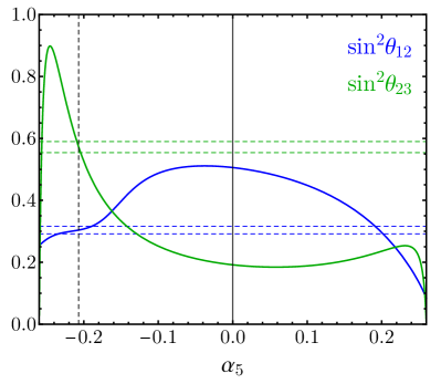
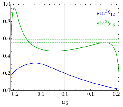
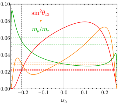
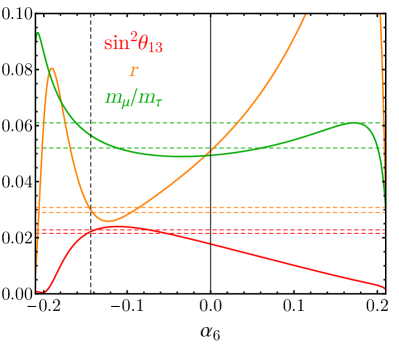
Figure 1: Dependence of the mixing angles and two mass ratios on $\alpha_{5}$ (left) and $\alpha_{6}$ (right), fixing all other input parameters to their best-fit values from Table 4. The horizontal dashed lines indicate the boundaries of the respective $1\sigma$ ranges from Table 1. The vertical dashed line in the left (right) panels stands for the best-fit value of $\alpha_{5}$ ($\alpha_{6}$) from Table 4.

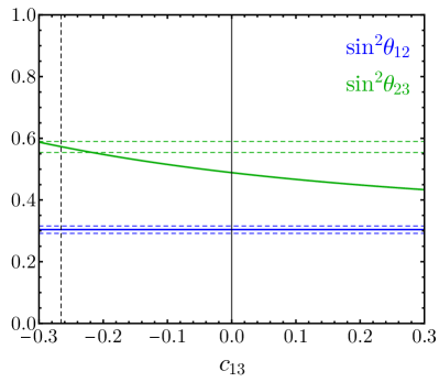
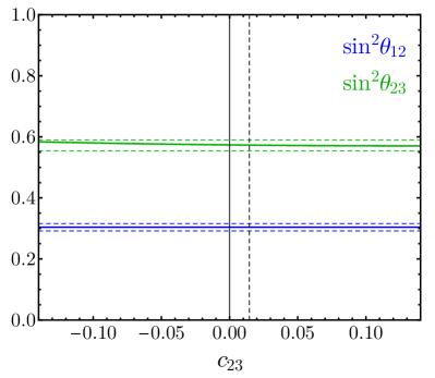
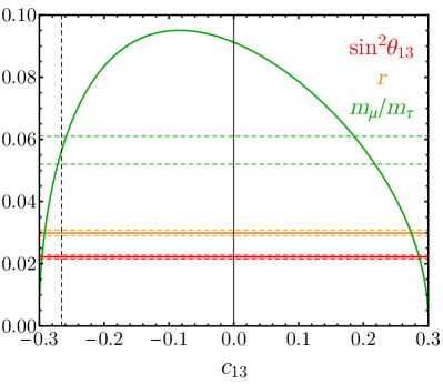
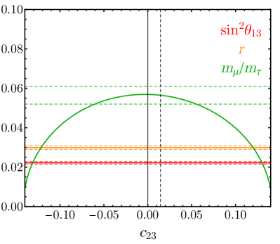
Figure 2: Dependence of the mixing angles and two mass ratios on $c_{13}$ (left) and $c_{23}$ (right), fixing all other input parameters to their best-fit values from Table 4. The horizontal dashed lines indicate the boundaries of the respective $1\sigma$ ranges from Table 1. The vertical dashed line in the left (right) panels stands for the best-fit value of $c_{13}$ ($c_{23}$) from Table 4.

We have analysed more in detail the dependence of the fitted observables on the parameters of the Kähler potential. In Figs. 1 and 2, we plot the values of the five dimensionless observables versus $\alpha_{5,6}$ and $c_{13,23}$, respectively . All other input parameters are fixed to their best-fit values as in Table 4. We see that the parameters $\alpha_{5}$ and $\alpha_{6}$ strongly impact the predictions for the mixing angles and the two mass ratios, $r$ and $m_{\mu}/m_{\tau}$, whereas $c_{13}$ and $c_{23}$ in $K_{E^{c}}$ mainly affect the predictions for $\sin^{2}\theta_{23}$ and $m_{\mu}/m_{\tau}$.

In conclusion, we see that a mass matrix of reduced rank at the self-dual point $\tau=i$ can explain the observed mass hierarchies in terms of $\mathcal{O}\left(1\right)$ Lagrangian parameters. At the same time, at least in the model considered here, moderately hierarchical Kähler and superpotential parameters are needed to fix the mixing angle predictions. Whether or not this is a general feature of this class of models is a question which definitely requires further investigation, but is beyond the scope of the present work. On the other hand, in order to get a fully realistic description of lepton masses we should still generate a non-vanishing electron mass, without perturbing too much the results achieved so far. We discuss this point in the next subsection.

4.3 Generating $m_{e}\neq 0$

Both the models discussed above yield, by construction, $m_{e}=0$. One can easily concoct mechanisms to generate the small electron mass without spoiling the other predictions. We give below two examples, where $m_{e}$ is generated by supersymmetry breaking and by dimension six operators, respectively.

If supersymmetry is broken by some $F$-term, fermion masses get corrected by the second term of eq. (7), which, as discussed below the same equation, scales as $m_{\mathrm{SUSY}}\,v/M$ for SM fermion masses (where $M$ is the SUSY breaking messenger scale). For instance, a Kähler interaction of the form:

$$K\supset\frac{1}{\Lambda^{2}}\chi^{\dagger}E_{i}^{c}\left[a_{i}(\tau)H_{d}+b_{i}(\tau)\widetilde{H}_{u}\right]L+\text{h.c.}\,,$$ (47)

where the superfield $\chi$ gets a supersymmetry breaking expectation value $\langle\chi\rangle=F\theta^{2}$, gives a contribution to the charged lepton Yukawa matrix proportional to $F/\Lambda^{2}$, which in turn generically induces an electron Yukawa coupling of the same order.

As a second possibility, one may generate $m_{e}\neq 0$ through the dimension six operator:

$$(E_{i}^{c}LH_{d})(H_{u}H_{d}),$$ (48)

whose Wilson coefficient should be a modular form of the appropriate weight. In order for this mechanism to work, we need to generalise the weight assignments in Table 2. We make the following requirements:

$$k_{L} =1-k_{u}\,,$$ (49)

$$k_{E^{c}} =3+k_{u}-k_{d}\,,$$ (50)

$$k_{u}+k_{d} \neq 0\,.$$ (51)

The first two conditions ensure that the superpotentials discussed in the previous subsections have weight zero; the last condition implies that the operator (48) has different weight from the corresponding renormalisable Yukawa term , so that it couples to a functionally independent modular form multiplet (making the resulting charged lepton mass matrix of rank three). Such a mechanism thus generates $m_{e}\sim v_{u}v_{d}^{2}/\Lambda^{2}$, where $\Lambda$ is the scale at which the operator in eq. (48) is generated.

While in some flavour models, the ratios $m_{e}/m_{\tau}$ and $m_{\mu}/m_{\tau}$ are associated to different powers of the same expansion parameter, we note that here the two ratios are associated to independent parameters.

5 Conclusion

Supersymmetric modular invariant theories offer an attractive framework to address the flavour puzzle. The role of flavour symmetry is played by modular invariance, regarded as a discrete gauge symmetry, thus circumventing the obstruction concerning fundamental global symmetries. The arbitrary symmetry breaking sector of the conventional models based on flavour symmetries is replaced by the moduli space. Yukawa couplings become modular forms, severely restricted by the matter transformation properties. So far this framework has delivered interesting preliminary results especially in the lepton sector, where neutrino masses and lepton mixing parameters can be efficiently described in terms of a limited number of input parameters.

Weak points in most of the existing constructions are the need of independent hierarchical parameters to describe charged lepton masses, the reduced predictability caused by a general form of the Kähler potential, and the absence of a reliable dynamical mechanism to determine the value of $\tau$ in the vacuum. As a matter of fact, in several models reproducing lepton masses and mixing parameters, the required value of $\tau$ is close to $i$, the self-dual point where the generator $S$ of the modular group and CP (if the Lagrangian is CP invariant) are unbroken. A small departure of $\tau$ from $i$ suffices to generate sizeable CP-violating effects in the lepton sector.

For these reasons, we were led to analyse more in detail the vicinity of $\tau=i$. Our goal was to show that a small deviation from the self-dual point can be responsible for the observed mass hierarchy $m_{e}\ll m_{\mu}\ll m_{\tau}$ and $\delta m^{2}\ll\Delta m^{2}$. At $\tau=i$, the theory has an exact $Z_{4}$ symmetry, generated by the element $S$ of the modular group. In the neighbourhood of $\tau=i$, the breaking of $Z_{4}$ can be fully described by the (small) spurion $\epsilon\approx\tau-i$, that flips its sign under $Z_{4}$. We explained how to exploit this residual $Z_{4}$ symmetry in order to obtain lepton mass matrices having reduced rank at $\tau=i$. This can be easily done with a suitable assignment of modular weights and representations for matter fields. There is a twofold advantage in this strategy. First, mass ratios that are forced to vanish at $\tau=i$ by the $Z_{4}$ symmetry are expected to acquire small values $\propto|\epsilon|^{n}$ $(n>0)$ near the self-dual point. Second, the reduced rank of the mass matrices can tame the contribution from a non-minimal Kähler potential, provided the metrics of the matter fields do not display large hierarchies.

To see whether this strategy can be successfully realised or not, we built a concrete model at level 3, where neutrinos get masses through the type I seesaw mechanism. The model predicts a normal mass ordering. The number of parameters exceeds the number of fitted observables and we cannot claim predictability. However, with $\tau$ being near $i$, mass ratios and mixing angles are reproduced with input parameters nearly of the same order of magnitude and matter kinetic terms display only a moderate hierarchy. We saw that the main contribution to the mass hierarchy can be induced by the singular mass matrix at the $Z_{4}$ symmetric point. In the model we considered, the Kähler potential and the other Lagrangian parameters are crucial in order to correctly reproduce the values of the mixing angles. While the $Z_{4}$ symmetry plays a fundamental role in all our discussion, we notice that our model could not have been realised in the context of a $Z_{4}$ flavour symmetry alone. In particular, the electron mass vanishes in the models we have considered due to the correlations among generic $Z_{4}$-invariant operators provided by the underlying modular invariance. Also the leading order values of the mixing angles are dictated by $Z_{4}$. We have discussed possible sources of a non-vanishing electron mass. While the models we formulated have clearly room for improvement, we consider them as a good starting point to naturally accommodate the observed fermion mass hierarchies within a modular invariant framework.

Note Added. Few weeks after completion of this work, ref. [43] appeared on the arXiv, in which the authors performed a systematic study of all fixed points, $\tau_{S}=i$, $\tau_{ST}=e^{2\pi i/3}$, and $\tau_{T}=i\infty$, assuming a minimal form of the Kähler potential. The points $\tau_{ST}$ and $\tau_{T}$ enjoy residual $Z_{3}\times Z_{2}$ and $Z_{N}\times Z_{2}$ symmetries, respectively (where $N$ is the level of modular forms used in the construction, $N=3$ in our work). It is found, in particular, that fermion mass hierarchies crucially depend on the decomposition of field representations under the residual symmetry group.

Appendix A Kähler potential quadratic in $Y^{(2)}$

In the real basis for the $\Gamma_{3}$ generators $S$ and $T$ in the 3-dimensional representation we employ in this work, $L^{\ast}$ and $Y^{(2)\ast}$ transform as triplets, i.e. $L^{\ast}\to\rho_{\mathbf{3}}(\tilde{\gamma})L^{\ast}$ and $Y^{(2)\ast}\to\rho_{\mathbf{3}}(\tilde{\gamma})Y^{(2)\ast}$. Thus, we can contract first $L^{\ast}$ with $L$ and $Y^{(2)\ast}$ with $Y^{(2)}$, and after that perform contractions of the obtained multiplets. Proceeding in this way, we obtain:

$$\left(L^{\ast}L\right)_{\mathbf{1}} =L^{\dagger}L\,,\qquad\left(L^{\ast}L\right)_{\mathbf{1^{\prime}}}=L^{\dagger}M_{\mathbf{1^{\prime}}}L\,,\qquad\left(L^{\ast}L\right)_{\mathbf{1^{\prime\prime}}}=L^{\dagger}M_{\mathbf{1^{\prime\prime}}}L\,,$$ (52)

$$\left(L^{\ast}L\right)_{\mathbf{3}_{S}} =\begin{pmatrix}L^{\dagger}M_{\mathbf{3}_{S}}^{(1)}L\\ L^{\dagger}M_{\mathbf{3}_{S}}^{(2)}L\\ L^{\dagger}M_{\mathbf{3}_{S}}^{(3)}L\end{pmatrix},\qquad\left(L^{\ast}L\right)_{\mathbf{3}_{A}}=\begin{pmatrix}L^{\dagger}M_{\mathbf{3}_{A}}^{(1)}L\\ L^{\dagger}M_{\mathbf{3}_{A}}^{(2)}L\\ L^{\dagger}M_{\mathbf{3}_{A}}^{(3)}L\end{pmatrix},$$ (53)

with the matrices $M_{\mathbf{r}}$ being

$$M_{\mathbf{1^{\prime}}} =\begin{pmatrix}1&0&0\\ 0&\omega^{2}&0\\ 0&0&\omega\end{pmatrix},\qquad M_{\mathbf{1^{\prime\prime}}}=\begin{pmatrix}1&0&0\\ 0&\omega&0\\ 0&0&\omega^{2}\end{pmatrix},$$ (54)

$$M_{\mathbf{3}_{S}}^{(1)} =\begin{pmatrix}0&0&0\\ 0&0&1\\ 0&1&0\end{pmatrix},\qquad M_{\mathbf{3}_{S}}^{(2)}=\begin{pmatrix}0&0&1\\ 0&0&0\\ 1&0&0\end{pmatrix},\qquad M_{\mathbf{3}_{S}}^{(3)}=\begin{pmatrix}0&1&0\\ 1&0&0\\ 0&0&0\end{pmatrix},$$ (55)

$$M_{\mathbf{3}_{A}}^{(1)} =\begin{pmatrix}0&0&0\\ 0&0&1\\ 0&-1&0\end{pmatrix},\qquad M_{\mathbf{3}_{A}}^{(2)}=\begin{pmatrix}0&0&-1\\ 0&0&0\\ 1&0&0\end{pmatrix},\qquad M_{\mathbf{3}_{A}}^{(3)}=\begin{pmatrix}0&1&0\\ -1&0&0\\ 0&0&0\end{pmatrix},$$ (56)

and $\omega=e^{2\pi i/3}$. The same equations hold for $\left(Y^{(2)\ast}Y^{(2)}\right)_{\mathbf{r}}$. Taking further invariant contractions of the obtained multiplets, we find

$$K_{L}=(2\operatorname{\texttt{Im}}\tau)^{-k_{L}}\mathbb{1}\phantom{{}=}$$

$${}+{}(2\operatorname{\texttt{Im}}\tau)^{k_{Y}-k_{L}}\bigg{\{} \alpha_{1}Y^{(2)\dagger}Y^{(2)}\mathbb{1}+\alpha_{2}\left[\left(Y^{(2)\dagger}M_{\mathbf{1^{\prime\prime}}}Y^{(2)}\right)M_{\mathbf{1^{\prime}}}+(Y^{(2)\dagger}M_{\mathbf{1^{\prime}}}Y^{(2)})M_{\mathbf{1^{\prime\prime}}}\right]$$

$$+\alpha_{3}\,i\left[\left(Y^{(2)\dagger}M_{\mathbf{1^{\prime\prime}}}Y^{(2)}\right)M_{\mathbf{1^{\prime}}}-\left(Y^{(2)\dagger}M_{\mathbf{1^{\prime}}}Y^{(2)}\right)M_{\mathbf{1^{\prime\prime}}}\right]$$

$$+\alpha_{4}\sum_{n=1}^{3}\left(Y^{(2)\dagger}M_{\mathbf{3}_{S}}^{(n)}Y^{(2)}\right)M_{\mathbf{3}_{S}}^{(n)}+\alpha_{5}\sum_{n=1}^{3}\left(Y^{(2)\dagger}M_{\mathbf{3}_{A}}^{(n)}Y^{(2)}\right)M_{\mathbf{3}_{A}}^{(n)}$$

$$+\alpha_{6}\sum_{n=1}^{3}i\left(Y^{(2)\dagger}M_{\mathbf{3}_{A}}^{(n)}Y^{(2)}\right)M_{\mathbf{3}_{S}}^{(n)}+\alpha_{7}\sum_{n=1}^{3}i\left(Y^{(2)\dagger}M_{\mathbf{3}_{S}}^{(n)}Y^{(2)}\right)M_{\mathbf{3}_{A}}^{(n)}\bigg{\}}\,,$$ (57)

where $\alpha_{j}$, $j=1\,,\dots\,,7$, are real coefficients, which accompany hermitian matrices. (We have used the fact that $M_{\mathbf{1^{\prime}}}^{\dagger}=M_{\mathbf{1^{\prime\prime}}}$, $M_{\mathbf{3}_{S}}^{(n)\dagger}=M_{\mathbf{3}_{S}}^{(n)}$, and $M_{\mathbf{3}_{A}}^{(n)\dagger}=-M_{\mathbf{3}_{A}}^{(n)}$.)

One of our assumptions is that the canonical form of $K_{L}$ is restored at $\operatorname{\texttt{Im}}\tau\to\infty$. The $q$-expansions of $Y_{i}$ in the real basis read:

$$Y_{1}(\tau) =\frac{1}{\sqrt{3}}\left(1-6q^{1/3}-18q^{2/3}+12q+\dots\right),$$ (58)

$$Y_{2}(\tau) =\frac{1}{\sqrt{3}}\left(1-6\omega q^{1/3}-18\omega^{2}q^{2/3}+12q+\dots\right),$$ (59)

$$Y_{3}(\tau) =\frac{1}{\sqrt{3}}\left(1-6\omega^{2}q^{1/3}-18\omega q^{2/3}+12q+\dots\right),$$ (60)

where $q=e^{2\pi i\tau}$. Thus, at $\operatorname{\texttt{Im}}\tau\to\infty$

$$Y_{1}=Y_{2}=Y_{3}\sim\frac{1}{\sqrt{3}}\,,$$ (61)

and $K_{L}$ has the following form:

$$K_{L}\sim\frac{1}{2\operatorname{\texttt{Im}}\tau}\mathbb{1}+\frac{2}{3}\operatorname{\texttt{Im}}\tau\begin{pmatrix}\frac{3}{2}\alpha_{1}&\alpha_{4}+i\alpha_{7}&\alpha_{4}-i\alpha_{7}\\ \alpha_{4}-i\alpha_{7}&\frac{3}{2}\alpha_{1}&\alpha_{4}+i\alpha_{7}\\ \alpha_{4}+i\alpha_{7}&\alpha_{4}-i\alpha_{7}&\frac{3}{2}\alpha_{1}\end{pmatrix},$$ (62)

where we have used $k_{L}=1$ and $k_{Y}=2$. To satisfy our assumption of the asymptotic behaviour of $K_{L}$, the coefficients $\alpha_{1}=\alpha_{4}=\alpha_{7}=0$. Thus, the number of free parameters in $K_{L}$ is reduced from seven to four. Then, the elements of $K_{L}$ from eq. (57) read:

$$\left(K_{L}\right)_{11} =\frac{1}{2\operatorname{\texttt{Im}}\tau}+2\operatorname{\texttt{Im}}\tau\left[2\alpha_{2}\lvert Y_{1}\rvert^{2}-\left(\alpha_{2}+\sqrt{3}\alpha_{3}\right)\lvert Y_{2}\rvert^{2}-\left(\alpha_{2}-\sqrt{3}\alpha_{3}\right)\lvert Y_{3}\rvert^{2}\right],$$ (63)

$$\left(K_{L}\right)_{22} =\frac{1}{2\operatorname{\texttt{Im}}\tau}+2\operatorname{\texttt{Im}}\tau\left[-\left(\alpha_{2}-\sqrt{3}\alpha_{3}\right)\lvert Y_{1}\rvert^{2}+2\alpha_{2}\lvert Y_{2}\rvert^{2}-\left(\alpha_{2}+\sqrt{3}\alpha_{3}\right)\lvert Y_{3}\rvert^{2}\right],$$ (64)

$$\left(K_{L}\right)_{33} =\frac{1}{2\operatorname{\texttt{Im}}\tau}+2\operatorname{\texttt{Im}}\tau\left[-\left(\alpha_{2}+\sqrt{3}\alpha_{3}\right)\lvert Y_{1}\rvert^{2}-\left(\alpha_{2}-\sqrt{3}\alpha_{3}\right)\lvert Y_{2}\rvert^{2}+2\alpha_{2}\lvert Y_{3}\rvert^{2}\right],$$ (65)

$$\left(K_{L}\right)_{12} =2\operatorname{\texttt{Im}}\tau\left(\alpha_{5}+i\alpha_{6}\right)\left[Y_{1}^{\ast}Y_{2}-Y_{1}Y_{2}^{\ast}\right],$$ (66)

$$\left(K_{L}\right)_{13} =2\operatorname{\texttt{Im}}\tau\left(\alpha_{5}-i\alpha_{6}\right)\left[Y_{1}^{\ast}Y_{3}-Y_{1}Y_{3}^{\ast}\right],$$ (67)

$$\left(K_{L}\right)_{23} =2\operatorname{\texttt{Im}}\tau\left(\alpha_{5}+i\alpha_{6}\right)\left[Y_{2}^{\ast}Y_{3}-Y_{2}Y_{3}^{\ast}\right].$$ (68)

For the sake of simplicity, we set further $\alpha_{2}=\alpha_{3}=0$. In this case, the diagonal entries of $K_{L}$ are not affected by the contributions containing modular forms, on the contrary to the off-diagonal elements. Thereby, we arrive at the form of $K_{L}$ in eqs. (43) and (44).

What concerns $K_{E^{c}}$, with the assignment of representations and weights given in Table 2, the most general Kähler potential quadratic in $Y^{(2)}$ reads

$$K_{E^{c}} =\frac{1}{8\left(\operatorname{\texttt{Im}}\tau\right)^{3}}\begin{pmatrix}c_{11}^{0}&c_{12}^{0}&0\\ c_{12}^{0\ast}&c_{22}^{0}&0\\ 0&0&c_{33}^{0}\end{pmatrix}$$

$$+\frac{1}{2\operatorname{\texttt{Im}}\tau}\begin{pmatrix}c_{11}Y^{(2)\dagger}Y^{(2)}&c_{12}Y^{(2)\dagger}Y^{(2)}&c_{13}Y^{(2)\dagger}M_{\mathbf{1^{\prime\prime}}}Y^{(2)}\\ c_{12}^{\ast}Y^{(2)\dagger}Y^{(2)}&c_{22}Y^{(2)\dagger}Y^{(2)}&c_{23}Y^{(2)\dagger}M_{\mathbf{1^{\prime\prime}}}Y^{(2)}\\ c_{13}^{\ast}Y^{(2)\dagger}M_{\mathbf{1^{\prime}}}Y^{(2)}&c_{23}^{\ast}Y^{(2)\dagger}M_{\mathbf{1^{\prime}}}Y^{(2)}&c_{33}Y^{(2)\dagger}Y^{(2)}\end{pmatrix}\,,$$ (69)

with $c_{ii}^{(0)}$ being real and $c_{ij}^{(0)}$, $i\neq j$, complex coefficients.

Taking into account that at $\operatorname{\texttt{Im}}\tau\to\infty$, the invariant combination $Y^{(2)\dagger}Y^{(2)}\sim 1$, whereas $X\equiv Y^{(2)\dagger}M_{\mathbf{1^{\prime\prime}}}Y^{(2)}$ and $X^{\ast}=Y^{(2)\dagger}M_{\mathbf{1^{\prime}}}Y^{(2)}$ decay exponentially, we find

$$K_{E^{c}}\sim\frac{1}{8\left(\operatorname{\texttt{Im}}\tau\right)^{3}}\begin{pmatrix}c_{11}^{0}&c_{12}^{0}&0\\ c_{12}^{0\ast}&c_{22}^{0}&0\\ 0&0&c_{33}^{0}\end{pmatrix}+\frac{1}{2\operatorname{\texttt{Im}}\tau}\begin{pmatrix}c_{11}&c_{12}&0\\ c_{12}^{\ast}&c_{22}&0\\ 0&0&c_{33}\end{pmatrix}.$$ (70)

In order to restore the canonical form of $K_{E^{c}}$ in the considered limit, $c_{12}^{0}=c_{12}=0$. Furthermore, we set $c_{ii}=0$ for simplicity. Finally, we can always make $c_{ii}^{0}=1$ by independent rescalings of $E_{i}^{c}$, $i=1,2,3$. Thus, we recover $K_{E^{c}}$ given by eqs. (45) and (46).

References

- [1] F. Feruglio and A. Romanino, “Lepton flavor symmetries,” Rev. Mod. Phys. 93 (Mar, 2021) 015007, arXiv:1912.06028 [hep-ph]. https://link.aps.org/doi/10.1103/RevModPhys.93.015007.
- [2] F. Feruglio, “Are neutrino masses modular forms?,” in From My Vast Repertoire …: Guido Altarelli’s Legacy, A. Levy, S. Forte, and G. Ridolfi, eds., pp. 227–266. 2019. arXiv:1706.08749 [hep-ph].
- [3] G.-J. Ding, F. Feruglio, and X.-G. Liu, “Automorphic Forms and Fermion Masses,” JHEP 01 (2021) 037, arXiv:2010.07952 [hep-th].
- [4] A. Baur, H. P. Nilles, A. Trautner, and P. K. Vaudrevange, “Unification of Flavor, CP, and Modular Symmetries,” Phys. Lett. B 795 (2019) 7–14, arXiv:1901.03251 [hep-th].
- [5] A. Baur, H. P. Nilles, A. Trautner, and P. K. Vaudrevange, “A String Theory of Flavor and ,” Nucl. Phys. B 947 (2019) 114737, arXiv:1908.00805 [hep-th].
- [6] T. Kobayashi and H. Otsuka, “Challenge for spontaneous violation in Type IIB orientifolds with fluxes,” Phys. Rev. D 102 no. 2, (2020) 026004, arXiv:2004.04518 [hep-th].
- [7] K. Ishiguro, T. Kobayashi, and H. Otsuka, “Landscape of Modular Symmetric Flavor Models,” arXiv:2011.09154 [hep-ph].
- [8] H. P. Nilles, S. Ramos-Sánchez, and P. K. Vaudrevange, “Eclectic Flavor Groups,” JHEP 02 (2020) 045, arXiv:2001.01736 [hep-ph].
- [9] H. P. Nilles, S. Ramos-Sanchez, and P. K. Vaudrevange, “Lessons from eclectic flavor symmetries,” Nucl. Phys. B 957 (2020) 115098, arXiv:2004.05200 [hep-ph].
- [10] H. P. Nilles, S. Ramos–Sánchez, and P. K. Vaudrevange, “Eclectic flavor scheme from ten-dimensional string theory – I. Basic results,” Phys. Lett. B 808 (2020) 135615, arXiv:2006.03059 [hep-th].
- [11] H. P. Nilles, S. Ramos-Sánchez, and P. K. Vaudrevange, “Eclectic flavor scheme from ten-dimensional string theory – II. Detailed technical analysis,” arXiv:2010.13798 [hep-th].
- [12] A. Baur, M. Kade, H. P. Nilles, S. Ramos-Sanchez, and P. K. Vaudrevange, “The eclectic flavor symmetry of the orbifold,” arXiv:2008.07534 [hep-th].
- [13] K. Ishiguro, T. Kobayashi, and H. Otsuka, “Spontaneous CP violation and symplectic modular symmetry in Calabi-Yau compactifications,” arXiv:2010.10782 [hep-th].
- [14] A. Baur, M. Kade, H. P. Nilles, S. Ramos-Sanchez, and P. K. Vaudrevange, “Siegel modular flavor group and CP from string theory,” arXiv:2012.09586 [hep-th].
- [15] M.-C. Chen, S. Ramos-Sánchez, and M. Ratz, “A note on the predictions of models with modular flavor symmetries,” Phys. Lett. B 801 (2020) 135153, arXiv:1909.06910 [hep-ph].
- [16] T. Kobayashi, N. Omoto, Y. Shimizu, K. Takagi, M. Tanimoto, and T. H. Tatsuishi, “Modular A4 invariance and neutrino mixing,” JHEP 11 (2018) 196, arXiv:1808.03012 [hep-ph].
- [17] J. C. Criado and F. Feruglio, “Modular Invariance Faces Precision Neutrino Data,” SciPost Phys. 5 no. 5, (2018) 042, arXiv:1807.01125 [hep-ph].
- [18] P. Novichkov, J. Penedo, S. Petcov, and A. Titov, “Modular S4 models of lepton masses and mixing,” JHEP 04 (2019) 005, arXiv:1811.04933 [hep-ph].
- [19] P. Novichkov, J. Penedo, S. Petcov, and A. Titov, “Generalised CP Symmetry in Modular-Invariant Models of Flavour,” JHEP 07 (2019) 165, arXiv:1905.11970 [hep-ph].
- [20] H. Okada and M. Tanimoto, “Towards unification of quark and lepton flavors in modular invariance,” arXiv:1905.13421 [hep-ph].
- [21] J. C. Criado, F. Feruglio, and S. J. King, “Modular Invariant Models of Lepton Masses at Levels 4 and 5,” JHEP 02 (2020) 001, arXiv:1908.11867 [hep-ph].
- [22] T. Kobayashi, T. Nomura, and T. Shimomura, “Type II seesaw models with modular symmetry,” Phys. Rev. D 102 no. 3, (2020) 035019, arXiv:1912.00637 [hep-ph].
- [23] H. Okada and M. Tanimoto, “Quark and lepton flavors with common modulus in modular symmetry,” arXiv:2005.00775 [hep-ph].
- [24] P. Novichkov, J. Penedo, and S. Petcov, “Double Cover of Modular for Flavour Model Building,” Nucl. Phys. B 963 (2021) 115301, arXiv:2006.03058 [hep-ph].
- [25] X. Wang, “Dirac neutrino mass models with a modular symmetry,” Nucl. Phys. B 962 (2021) 115247, arXiv:2007.05913 [hep-ph].
- [26] H. Okada and M. Tanimoto, “Spontaneous CP violation by modulus in model of lepton flavors,” arXiv:2012.01688 [hep-ph].
- [27] S. J. King and S. F. King, “Fermion mass hierarchies from modular symmetry,” JHEP 09 (2020) 043, arXiv:2002.00969 [hep-ph].
- [28] H. Okada and M. Tanimoto, “Modular invariant flavor model of and hierarchical structures at nearby fixed points,” Phys. Rev. D 103 no. 1, (2021) 015005, arXiv:2009.14242 [hep-ph].
- [29] P. Novichkov, J. Penedo, S. Petcov, and A. Titov, “Modular A5 symmetry for flavour model building,” JHEP 04 (2019) 174, arXiv:1812.02158 [hep-ph].
- [30] P. P. Novichkov, S. T. Petcov, and M. Tanimoto, “Trimaximal Neutrino Mixing from Modular A4 Invariance with Residual Symmetries,” Phys. Lett. B 793 (2019) 247–258, arXiv:1812.11289 [hep-ph].
- [31] S. F. King and Y.-L. Zhou, “Trimaximal TM1 mixing with two modular groups,” Phys. Rev. D 101 no. 1, (2020) 015001, arXiv:1908.02770 [hep-ph].
- [32] G.-J. Ding, S. F. King, X.-G. Liu, and J.-N. Lu, “Modular S4 and A4 symmetries and their fixed points: new predictive examples of lepton mixing,” JHEP 12 (2019) 030, arXiv:1910.03460 [hep-ph].
- [33] J. Gehrlein and M. Spinrath, “Leptonic Sum Rules from Flavour Models with Modular Symmetries,” arXiv:2012.04131 [hep-ph].
- [34] S. Ferrara, D. Lust, A. D. Shapere, and S. Theisen, “Modular Invariance in Supersymmetric Field Theories,” Phys. Lett. B 225 (1989) 363.
- [35] S. Ferrara, D. Lust, and S. Theisen, “Target Space Modular Invariance and Low-Energy Couplings in Orbifold Compactifications,” Phys. Lett. B 233 (1989) 147–152.
- [36] X.-G. Liu, C.-Y. Yao, B.-Y. Qu, and G.-J. Ding, “Half-integral weight modular forms and application to neutrino mass models,” Phys. Rev. D 102 no. 11, (2020) 115035, arXiv:2007.13706 [hep-ph].
- [37] A. Brignole, F. Feruglio, and F. Zwirner, “Aspects of spontaneously broken N=1 global supersymmetry in the presence of gauge interactions,” Nucl. Phys. B 501 (1997) 332–374, arXiv:hep-ph/9703286.
- [38] G. Ross and M. Serna, “Unification and fermion mass structure,” Phys. Lett. B 664 (2008) 97–102, arXiv:0704.1248 [hep-ph].
- [39] I. Esteban, M. C. Gonzalez-Garcia, M. Maltoni, T. Schwetz, and A. Zhou, “The fate of hints: updated global analysis of three-flavor neutrino oscillations,” JHEP 09 (2020) 178, arXiv:2007.14792 [hep-ph].
- [40] I. Esteban, M. C. Gonzalez-Garcia, M. Maltoni, T. Schwetz, and A. Zhou, “NuFIT 5.0: Three-neutrino fit based on data available in July 2020.” WWW.NU-FIT.ORG.
- [41] T. Kobayashi, Y. Shimizu, K. Takagi, M. Tanimoto, T. H. Tatsuishi, and H. Uchida, “ violation in modular invariant flavor models,” Phys. Rev. D 101 no. 5, (2020) 055046, arXiv:1910.11553 [hep-ph].
- [42] T. Asaka, Y. Heo, and T. Yoshida, “Lepton flavor model with modular symmetry in large volume limit,” Phys. Lett. B 811 (2020) 135956, arXiv:2009.12120 [hep-ph].
- [43] P. P. Novichkov, J. T. Penedo, and S. T. Petcov, “Fermion mass hierarchies, large lepton mixing and residual modular symmetries,” JHEP 04 (2021) 206, arXiv:2102.07488 [hep-ph].