Calculating the polarization in bi-partite lattice models: application to an extended Su-Schrieffer-Heeger model

Abstract

We address the question of different representation of Bloch states for lattices with a basis, with a focus on topological systems. The representations differ in the relative phase of the Wannier functions corresponding to the diffferent basis members. We show that the phase can be chosen in such a way that the Wannier functions for the different sites in the basis both become eigenstates of the position operator in a particular band. A key step in showing this is the extension of the Brillouin zone. When the distance between sites within a unit cell is a rational number, $p/q$, the Brillouin extends by a factor of $q$. For irrational numbers, the Brillouin zone extends to infinity. In the case of rational distance, $p/q$, the Berry phase “lives” on a cyclic curve in the parameter space of the Hamiltonian, on the Brillouin zone extended by a factor of $q$. For irrational distances the most stable way to calculate the polarization is to approximate the distance as a rational sequence, and use the formulas derived here for rational numbers. The use of different bases are related to unitary transformations of the Hamiltonian, as such, the phase diagrams of topological systems are not altered, but each phase can acquire different topological characteristics when the basis is changed. In the example we use, an extended Su-Schrieffer-Heeger model, the use of the diagonal basis leads to toroidal knots in the Hamiltonian space, whose winding numbers give the polarization.

I Introduction

Recently, several papers investigated Bena09 ; Watanabe18 the different representation of the wave function and physical observables when the underlying model is a lattice with a basis. This fundamental question is important per se, moreover, such models have been the subject of intense research in the last decades, exemplified by graphene, the kagome, or Lieb lattices, and others. The canonical models for topological insulators Bernevig13 ; Kane13 ; Asboth15 are all lattices with bases: the Haldane, Haldane88 Kane-Mele, Kane05a ; Kane05b Su-Schrieffer-Heeger Su79 models are some of the most fundamental ones.

Bena and Montambaux Bena09 have studied the two commonly used bases of the graphene lattice. The difference between the two is that in one (basis $I$), the different position of the sites within a unit cell are not explicit (they are taken to be the same, the position of the unit cell itself), whereas in the other (basis $II$), the positions of the different sites within a unit cell are explicit. What is meant by this is that in $I$, the Wannier functions corresponding to the different basis members have the same phase, while in $II$ their relative phase depends on the distance between them. Bena and Montambaux Bena09 show that in the case of the graphene lattice, although the Hamiltonian and operators take different forms in the two bases, important physical quantities, such as the density or the density of states, as well as the low-energy theory, are unchanged. However, care must be taken in using the correct construction of observables, once a representation of the wave functions is chosen.

Watanabe and Oshikawa Watanabe18 have taken up this question more recently, and they show that, while the precise form of the current operator does depend on the choice of basis, the quantized charge pumped during an adiabatic cycle Thouless82 is unchanged. Note that the current operator is intimately related to the phase of the wave function, in particular the relative phase wave functions centered on different sites may exhibit. Also note that the charge pumped is a topological invariant, which remains the same in different bases.

In this paper we reconsider the question of basis dependence in lattice models in the context of modern polarization theory with a focus on topological systems. We compare the two bases used in Ref. Bena09 , and show that one corresponds to a linear combination of Wannier functions which are eigenfunctions of the position operator. When the distance between the basis sites is a rational number $p/q$, the Brillouin zone has to be extended by a factor of $q$ to derive the above result. If the distance is irrational, then the Brillouin zone has to be extended to the whole real line.

We then turn to the question of topological phase transitions in the two bases. As an example system we consider an extended Su-Schrieffer-Heeger Su79 (SSH) model. When the $k$-space Hamiltonian is written considering distance dependence explicitly the three-dimensional curve $d_{x},d_{y},d_{z}$ (see Eq. 7) is not a closed curve. When the distance between basis sites is a rational number ($p/q$) extending the Brillouin zone by a factor of $q$ closes the curve, and an expression for the polarization Berry phase Berry84 ; Zak89 ; King-Smith93 ; Resta98 ; Resta00 can be derived. In the irrational case a closed $d_{x},d_{y},d_{z}$-curve results only if the Brillouin zone is extended to infinity. For this reason, calculation of the irrational case is not straightforward. We show that a stable calculation results if the irrational distance is approximated as a rational sequence.

Implementing the dependence of the Hamiltonian on the distance between basis sites proceeds through a unitary transformation. As such, the Hamiltonian can acquire auxiliary topological features. In the model we study, the $d_{x},d_{y},d_{z}$-curve traces out a toroidal knot, and the ratio of the winding numbers of the knot give the polarization. However, the phase diagram itself is not altered, since these topological characteristics are merely different representations of the phases of the original extended SSH model.

In the next section we discuss the two different bases used in lattices with a basis. In section III the extended SSH model is described. In section IV the change of basis is discussed in the context of the extended SSH model. In section V our results are presented, and in section VI we conclude our work.

II Polarization and choice of representation

It is well-known Blount62 ; Kivelson82 that Wannier functions in systems without a basis are eigenstates of the position operator within a given band. Here we show that in a lattice with a basis, one of the representations of the wave-function studied by Bena and Montambaux Bena09 leads to position eigenstates.

We consider a one-dimensional system whose potential obeys $V(x)=V(x+1)$ (in other words we take the length of a unit cell as unity). The unit cell consists of a two-site basis. We chose the distance between the two internal sites to be $p/q$, a rational number, and we extend the Brillouin zone by a factor of $q$. This step is justified below.

In this case, the two commonly used bases Bena09 can be written as

$$u_{k}^{I}(x)= \sum\limits_{m=-\infty}^{\infty}e^{ik(m-x)}\left[w_{a}(x-m)+w_{b}\left(x-m-\frac{p}{q}\right)\right]$$

$$u_{k}^{II}(x)= \sum\limits_{m=-\infty}^{\infty}\left[e^{ik(m-x)}w_{a}(x-m)+e^{ik(m+p/q-x)}\times\right.$$ (1)

$$\left.\times w_{b}\left(x-m-\frac{p}{q}\right)\right].$$

The functions $u_{k}^{I}(x)$ and $u_{k}^{II}(x)$ are periodic Bloch functions. $u_{k}^{I}(x)$ is the more standard approach, and it appears Ashcroft76 in textbooks. $w_{a}(x),w_{b}(x)$ are two different localized Wannier functions. In the extended SSH model we study below, they differ only in having their centers displaced with respect to each other.

Following Zak Zak89 we derive the geometric phase which arises upon integrating the connection across the Brillouin zone. We define a geometric phase of the Zak type, in the extended Brillouin zone as:

$$\gamma=\frac{i}{2\pi q}\int_{-q\pi}^{q\pi}dk\langle u_{k}|\partial_{k}|u_{k}\rangle.$$ (2)

Using $u_{k}^{I}$ the Zak phase becomes

$$\gamma_{I}=\int_{-\infty}^{\infty}dxx\left|w_{a}(x)+w_{b}\left(x-\frac{p}{q}\right)\right|^{2},$$ (3)

whereas with $u_{k}^{II}$

$$\gamma_{II}=\int_{-\infty}^{\infty}dxx\left(|w_{a}(x)|^{2}+|w_{b}(x)|^{2}\right).$$ (4)

In deriving $\gamma_{II}$, we made use of the fact that

$$\frac{1}{2\pi q}\int_{-\pi q}^{\pi q}dk\exp\left(ik(n-n^{\prime})/q\right)=\delta_{nn^{\prime}}.$$ (5)

Comparing $\gamma_{I}$ and $\gamma_{II}$ we see that the second Bloch basis function, $u_{k}^{II}$ is a diagonal basis for the position operator in a periodic system, since the result is a simple sum of Wyckoff positions for the two different Wannier functions. It is due to Eq. (5) that the cross terms in $\gamma_{II}$ disappear, but only of the Brillouin zone is extended by a factor of $q$.

It is instructive to consider the effect of inversion symmetry on either $\gamma$. In the original work of Zak Zak89 , where the sites are equivalent, two types of inversion symmetries were considered, site-inversion and bond-inversion. The former gives a Zak phase of zero, while the latter gives $\pi$, which corresponds to a polarization of $qa/2$ ($a$ is the length of the unit cell). In our case, there are also two types of inversion. If the sites of the model are a distance $p/q$ apart, one can consider inverting around the midpoint of the $p/q$ bond, or the $1-p/q$ bond. In the former case it holds that $w_{c}(-x+p/q)=\pm w_{c}(x)$ for both $c=a,b$, which leads to $\gamma=\frac{p}{2q}$ (for both $I$ and $II$). In deriving this one can follow the stame steps as ZakZak89 . Inverting around the other bond center leads to $w_{c}(-x-1+p/q)=\pm w_{c}(x)$, from which it follows that $\gamma=\frac{p-q}{2q}$ (again for both $I$ and $II$).

In the case of irrational distance, the Brillouin zone has to be extended to the range $(-\infty,\infty)$. When this is done, Eq. (5) eliminates the cross terms and leads to $\gamma_{II}$.

III Model

The full model we consider is an extension of the well-known Su-Schrieffer-Heeger model Su79 . It is a bi-partite lattice model ($A$ and $B$ sublattices), whose Hamiltonian has the form,

$$\hat{H}=-\sum_{i=1}^{L}[Jc_{i}^{\dagger}d_{i}+J^{\prime}d_{i}^{\dagger}c_{i+1}+iKc_{i}^{\dagger}c_{i+1}-iKd_{i}^{\dagger}d_{i+1}+\mbox{H.c.}],$$ (6)

where $L$ denotes the number of unit cells, $c_{i}$($c_{i}^{\dagger}$) denote the annihiliation(creation) operators on the $A$ site of the $i$th unit cell, and $d_{i}$($d_{i}^{\dagger}$) denote the same for the $B$ site of the $i$th unit cell. We take the length of a unit cell to be unity. An extended SSH model of a different kind, with real second nearest neighbor hoppings, was invesigated by Li et al. Li14 .

When $K=0$ the SSH model is recovered. The third and fourth terms in Eq. (6) correspond to second nearest neighbor hoppings (hoppings within one sublattice). A Peierls phase of $\pi/2$ and $-\pi/2$ is applied along these hoppings, the former for sublattice $A$, the latter for sublattice $B$. These second nearest neighbor hoppings play a similar role to those in the Haldane model Haldane88 . There and in Eq. (6) the Peierls phases of second nearest neighbor hoppings point in opposite directions on the two sublattices. The consequence of this term is that for gapped phases and finite $K$ there is persistent current in the system, but the currents on the different sublattices cancel, and insulation results. If $K$ changes sign, the direction of the persistent currents on the different sublattices also change sign. In this sense, the model can be viewed as an example of Kohn’s tenet Kohn64 . This tenet states that insulation in a quantum system is not a function of localization of individual charge carriers, but ultimately results from many-body localization, or the localization of the center of mass of all the charge carriers. Individually, charge carriers can be quite mobile, as long as the center of mass is localized.

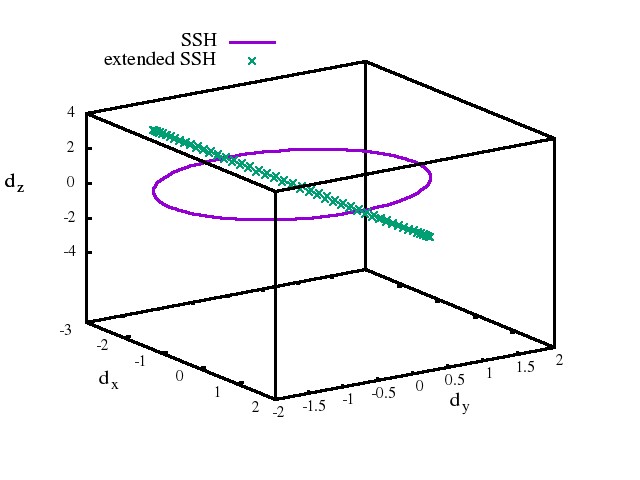
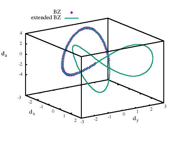
Figure 1: Curves traced out by the parameters of the Hamiltonian $d_{x},d_{y},d_{z}$ as $k$ traverses Brillouin zone for the usual SSH and the extended SSH model. Upper panel: SSH model and extended SSH model in the usual basis. Lower panel: extended SSH model in the distance dependent basis comparing the first Brilllouin zone to the extended Brillouin zone.

According to the symmetry classification Altland97 ; Schnyder08 of topological insulators, the SSH model, which exhibits time reversal, particle-hole, and chiral symmetries, falls into the BDI class, which in one dimension is a $\mathbb{Z}$-topological system. After the addition of the second nearest neighbor hopping term in Eq. (7) only the particle-hole symmetry remains, and the model falls in the D symmetry class, which is a $\mathbb{Z}_{2}$ system. The gap closure points of the SSH remain (they occur at $k=0,\pi$), and we show below that topological edge states still arise.

Fourier transforming Eq. (6) results in

$$\hat{H}=\sum_{k}H_{k}=\sum_{k}[d_{x}(k)\sigma_{x}+d_{y}(k)\sigma_{y}+d_{z}(k)\sigma_{z}],$$ (7)

where $\sigma_{x},\sigma_{y},\sigma_{z}$ denote the Pauli matrices, and

$$d_{x}(k) = -J-J^{\prime}\cos(k),$$ (8)

$$d_{y}(k) = -J^{\prime}\sin(k),$$

$$d_{z}(k) = 2K\sin(k).$$

Written this way, we see that gap closure occurs at $k=\pi$ if $J=J^{\prime}$. The upper panel Fig. 1 shows the curves traced out by $d_{x},d_{y},d_{z}$ as $k$ traverses the Brillouin zone for the usual SSH model ($J=1.25,J^{\prime}=1.75$) with $K=0$ and an example of the extended one, with $K=2$. The former forms a circle in the $xy$-plane, the latter is a circle with a tilted axis (axis along the $yz$-plane). Both circles cross the $x$-axis itself in two places at the same points. This means, that by varying the ratio of $J/J^{\prime}$ it is possible to close the gap in both models, and encounter topological phase transitions.

We can also develop a continuum approximation, the usual way Jackiw76 ,

$$H=it\partial_{x}\sigma_{x}+iK\partial_{x}\sigma_{y}+2\delta t\sigma_{z},$$ (9)

where we used the parametrization:

$$t = \frac{J+J^{\prime}}{2}$$ (10)

$$\delta t = \frac{J^{\prime}-J}{2}$$

We can solve for zero energy eigenstates of the form

$$\begin{pmatrix}\Psi_{A}(x)\\ \Psi_{B}(x)\end{pmatrix}.$$ (11)

The zero energy solution is

$$\Psi_{A/B}^{\prime\prime}(x)=\frac{4\delta t^{2}}{t^{2}+K^{2}}\Psi_{A/B}(x).$$ (12)

The solutions are exponentials. If the system is extended, these solutions diverge, hence they are unnormalizable. If the system has open boundary conditions, exponential solutions can be normalized, since they can start at one of the boundaries and decay towards the bulk. Therefore zero-energy states are possile. The sign of $\delta t$ determines the direction of decay, in other words, the side of the finite system on which the edge state is located. The signs of $t$ and $K$ are irrelevant.

It is interesting to compare the above results to those of Jackiw and Rebbi Jackiw76 . There a first order differential equation is solved for a function multiplying a $\sigma_{z}$ eigenstate, while in our case each component of the Pauli spinor satisfies the same second order differential equation. Our calculations below on the lattice model (see Fig. 3) bear out the predictions of our continuum theory.

IV Implementation of distance dependence

We take the shortest distance between the two sublattices to be $p/q$, where $p$ and $q$ are co-prime integers. The Hamiltonian in $k$-space can be shown to be:

$$d_{x}(k) = -J\cos\left[k\left(\frac{p}{q}\right)\right]-J^{\prime}\cos\left[k\left(1-\frac{p}{q}\right)\right]$$ (13)

$$d_{y}(k) = J\sin\left[k\left(\frac{p}{q}\right)\right]-J^{\prime}\sin\left[k\left(1-\frac{p}{q}\right)\right]$$

$$d_{z}(k) = 2K\sin(k).$$

This Hamiltonian can also be derived from the original one (Eq. (7)) by

$$H_{k}\rightarrow\exp\left(ik\frac{\sigma_{z}}{2}\frac{p}{q}\right)H_{k}\exp\left(-ik\frac{\sigma_{z}}{2}\frac{p}{q}\right),$$ (14)

a rotation by angle $kp/q$ around the $z$ axis. We also note that the vector function $[d_{x},d_{y},d_{z}]$ has a period of $2\pi q$, rather than the usual $2\pi$.

Due to the fact that the distance dependence coincides with a rotation, a qualitative difference between the case of rational and irrational distances arises. As is known Asboth15 ; Kane13 , the curve traced out by the SSH model on the $d_{x}-d_{y}$ plane is an ellipse whose center, in general, lies on the $d_{x}$ axis. Implementing the distance dependence will generate a different curve. A closed curve can be obtained if the distance between sublattice sites is taken to be a rational number ($p/q$ with $p$ and $q$ coprimes), and the Brillouin zone is extended to $2\pi q$. Observables related to the Berry (Zak) phase (polarization, topological invariants) depend on the curve being closed, since these physical quantities are integrals over a connection over a closed curve (usually the Brillouin zone).

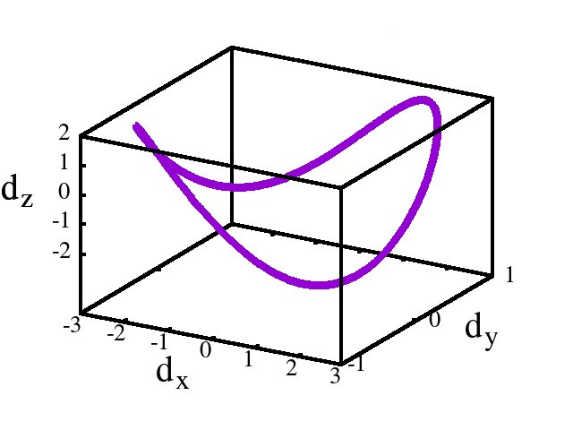
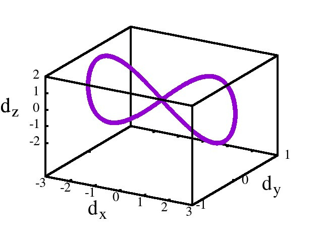
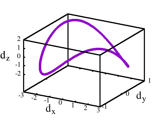
Figure 2: Curves traced out by the parameters of the Hamiltonian $d_{x},d_{y},d_{z}$ as $k$ traverses the extended Brillouin zone for the $\frac{p}{q}=\frac{1}{2}$ case. The Hamiltonian parameters are $K=1$ in all cases, and $J=1,J^{\prime}=2$ (upper panel), $J=1.5,J^{\prime}=1.5$ (middle panel), $J=2,J^{\prime}=1$ (lower panel). The curves of the upper and lower panels appear equivalent, but the orientation of the curves changes as the gap closure point (the figure-8 of the middle panel) is crossed.

Let us rewrite the $d$-curve of Eq. (13) with a scaled wave vector, $k=q\kappa$, as

$$d_{x}(\kappa) = -\cos(\kappa p)\left[J+J^{\prime}\cos(\kappa q)\right]$$

$$-\sin(\kappa p)J\sin(\kappa q),$$

$$d_{y}(\kappa) = +\sin(\kappa p)\left[J+J^{\prime}\cos(\kappa q)\right]$$

$$-\cos(\kappa p)J^{\prime}\sin(\kappa q),$$

$$d_{z}(\kappa) = +2K\sin(\kappa q).$$

This curve exists on the surface of a torus, albeit, not a torus of the usual parametrization, and the curve itself is a toroidal knot (see examples in Figs. 2, 4, 5).

The fundamental group Nakahara03 of the torus is $\pi_{1}(T^{2})=\pi_{1}(S^{1})\oplus\pi_{1}(S^{1})=\mathbb{Z}\oplus\mathbb{Z}$, meaning that homotopically equivalent classes of loops on the torus can be characterized by two integers. In Eq. (IV) the two integers are $p,q$, and in this parametrization they are toroidal winding numbers. A torus knot is obtained by a trajectory which loops around the hole of the torus an integer number of times ($w_{1}=p$), while it makes an integer number of rotations around the “body” of the torus itself ($w_{2}=q$). As argued in the previous section, the ratio of winding numbers is proportial to the polarization. A curve parametrized as Eq. (IV) traces out a toroidal knot for a given integer pair $p,q$, even if $p$ and $q$ are not co-primes. If they are co-primes then there is only one curve, if they are not, then the same curve is traced more than once, as many times as the common divisor of $p$ and $q$. In the original parametrization, Eq. (13), the rescaling leads to the same curves for a given $p,q$.

Alternatively, one can define $r=q-p$ in Eq. (13), and arrive at a different curve, similar in form to Eq. (IV). In this case the winding numbers will be $w_{1}=r$ and $w_{2}=q$. Thus, we can write the two different fractionally quantized polarization results of the previous section as:

$$\mathfrak{P}=-\frac{e}{2}\frac{w_{1}}{w_{2}}.$$ (16)

The lower panel of Fig. 1 shows two curves for this extended model, one using a normal Brillouin zone ($-\pi,\pi$), the other an extended one ($-q\pi,q\pi$) (model parameters are $J=1.25,J^{\prime}=1.75,K=2$ and $p/q=1/3$ in both cases). The former curve is open, the latter is a closed curve, a toroidal knot.

In our calculations below the Brillouin zone is stretched by a factor of $q$, and we take every $q$th point in $k$ space in this enlarged Brillouin zone. The starting point for the polarization expression is the scalar product

$$Z_{q}=\langle\Psi|\exp\left(i\frac{2\pi\hat{X}}{L}q\right)|\Psi\rangle.$$ (17)

Following the steps of Resta Resta98 , in a band insulator we have

$$Z_{q}=\prod_{s=0}^{L-1}\mbox{det}S(k_{qs},k_{q(s+1)}).$$ (18)

where

$$S_{m,m^{\prime}}(k_{qs},k_{q(s+1)})=\int_{0}^{L}dx\hskip 2.84544ptu^{*}_{k_{qs},m}(x)u_{k_{q(s+1)},m^{\prime}}(x),$$ (19)

where $u_{k_{qs},m}(x)$ denote the periodic Bloch functions of band $m$, and $k_{qs}=2\pi qs/L$. In our numerics we calculate the polarization via

$$\mathfrak{P}=-\frac{e}{2\pi}\mbox{Im}\ln\prod_{s=0}^{L-1}[\mbox{det}S(k_{qs},k_{q(s+1)})]^{\frac{1}{q}}.$$ (20)

This definition is important from the point of view of implementation, because the $\frac{1}{q}$ power keeps the terms in the Berry phase between $0$ and $2\pi$, and provides the correct fractional polarization.

Again the question remains, whether irrational distances can be handled. The difficulty in this case is that the Brillouin zone has to be extended to infinity. Two methods suggest themselves. One, use the irrational distance itself in place of $p/q$, and compare larger and larger Brillouin zones. In this case, the curve in the $d_{x},d_{y},d_{z}$ curve will be open. Another way would be to approximate the irrational distance as the limit of a sequence of rational numbers, and investigate the limit of Eq. (20) along that sequence. Below a comparison is presented for the case when the distance is the inverse of the golden ratio.

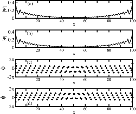
Figure 3: Calculation for a system with open boundary conditions with $L=100$ (meaning also that there are $100$ states). The parameters of the Hamiltonian are $J=1.25,J^{\prime}=1.75,K=2.0$. The minimum distance between sublattices is $p/q=1/3$. The figure show: (a) the zero energy state number $50$, (b) the zero energy state number $51$, (c) the phase of the wave function as a function of lattice site for state number $50$, and (d) the phase of the wave function as a function of lattice site for state number $51$.

V Results

The curves traced out by the parameters of the Hamiltonian ($d_{x},d_{y},d_{z}$) are shown in Fig. 2 for three cases: $J=1,J^{\prime}=2$; $J=1.5,J^{\prime}=1.5$; $J=2,J^{\prime}=1$ ($K=1$ in all three cases) for $p=1,q=2$. The topological transition occurs at $J=1.5,J^{\prime}=1.5$, where the curve traces out a figure$-8$, with a crossing point at the origin. The curves on the different sides of this phase diagram (the uppermost and lowermost panels) can be transformed into each other via a rotation by $\pi/2$. Since the orientation of the curves (the sense of rotation around the $d_{z}$-axis) does change when crossing the phase boundary the winding number goes from one to minus one. This corresponds to a polarization reversal from $\mathfrak{P}=e/4$ to $\mathfrak{P}=-e/4$, as expected.

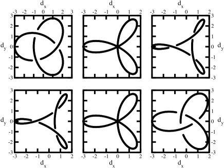
Figure 4: Curves traced out by the parameters of the Hamiltonian $d_{x},d_{y},d_{z}$ as $k$ traverses the extended Brillouin zone. The upper(lower) set of plots show the case $\frac{p}{q}=\frac{1}{3}$($\frac{p}{q}=\frac{2}{3}$), where the parameters of the Hamiltonian are, left: $J^{\prime}=1.75,J=1.25$, center:$J=1.5,J^{\prime}=1.5$, and right:$J^{\prime}=1.25,J=1.75$ ($K=1$ in all cases).

Fig. 3 presents a study of how edge states arise in a system with open boundary conditions. The parameters of the Hamiltonian are $J=1.25,J^{\prime}=1.75,K=2.0$ with $p=1$ and $q=3$. The upper two panels ((a) and (b)) show the two zero energy wave functions which are localized at the edges. The system is fairly small $L=100$, and the paramater $K$ is fairly large, giving rise to edge state wavefunctions with a sizable finite component even halfway through the lattice, however, as the size is increased and/or if $K$ is decreased the bulk compoment of the state decreases. These results are consistent with our previous derivation (Eq. (9)). For a system with $J^{\prime}<J$ edge-states are not found. The bottom panels ((c) and (d)) show the phase of the zero energy wave functions. The phases of both edge states oscillate when going towards the center from the edges. The left and right sides mirror each other, and a sudden change occurs at and within a few sites near the center of the system.

In Figs. 4 and 5 the $d_{x},d_{y},d_{z}$ curves are shown for various values of $p$ and $q$. The Hamiltonian parameters are as follows: left $J^{\prime}=1.75,J=1.25$, center $J^{\prime}=1.5,J=1.5$, and right $J^{\prime}=1.25,J=1.75$. $K=1.0$ for all cases. The plots are knot diagrams Adams01 , two dimensional knot representations, arrived at by projecting the curve onto the $d_{x}-d_{y}$ plane, but indicating which strand is below the other at crossings. Other than the plots in the center in both figures, neither of which are knots, the left and right plots show torus knots. For example, in the top left figure of Fig. 5, the curve winds around $w_{1}=4$ times while it makes $w_{2}=5$ revolutions around the body of the torus.

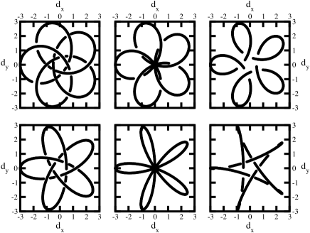
Figure 5: Curves traced out by the parameters of the Hamiltonian $d_{x},d_{y},d_{z}$ as $k$ traverses the extended Brillouin zone. The upper(lower) set of plots show the case $\frac{p}{q}=\frac{1}{5}$($\frac{p}{q}=\frac{2}{5}$). The parameters of the Hamiltonian are, left: $J^{\prime}=1.75,J=1.25$, center:$J=1.5,J^{\prime}=1.5$, and right:$J^{\prime}=1.25,J=1.75$ ($K=1$ in all cases).

The center plots in both Figs. 4 and 5 show curves for the topological phase transition. These curves do not form knots, they cross at the origin, which is the gap closure point. It is obvious that these center plots “connect” the two topologically distinct phases on either side of the phase transition. At the phase transition the torus surface on which the curves “live” is a horn torus. On either side of the horn torus, the curves reconnect, in a manner reminiscent of “partner switching” of edge states in the Kane-Mele model Kane05a ; Kane05b .

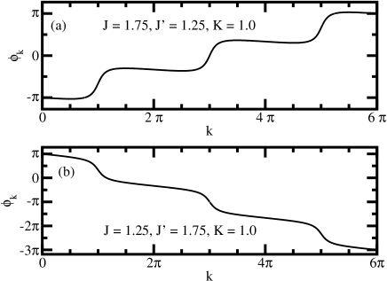
Figure 6: The trajectory of $\phi_{k}$ a parameter which defines the wave-function (Eq. (21)) across the extended Brillouin zone for a trivial (a) and a topological (b) case. As $k$ sweeps across the extended Brillouin zone $\phi_{k}$ increases by $2\pi$ in the trivial, and $-4\pi$ in the topological system.

The upper plots in Fig. 4 are for $p=1$, the lower ones are $p=2$. The upper left plot shows a trefoil knot with $w_{1}=2$, $w_{2}=-3$. The upper right plot shows an un-knot with $w_{1}=1$, $w_{2}=3$. Even though there are crossings on this curve, they can be eliminated by type I Reidemeister moves Adams01 , one of three modifications on two-dimensional representations of knots which leave knot invariants unaltered. The knot invariants (in this case the two winding numbers) are not altered by these modifications (if all three twists are eliminated).

The topological phase transition connects the two states. In the insulating phases Eq. (16) is recovered. In the lower set the $J^{\prime}>J$ curve exhibits the unknot ($w_{1}=1,w_{2}=-3$), and the $J>J^{\prime}$ the trefoil knot ($w_{1}=2,w_{2}=3$), again consistent with Eq. (16).

In Fig. 5 the $d_{x},d_{y},d_{z}$ curves are shown for various $q=5$ cases. The upper plots are $p=1$, the lower ones are $p=2$. The phase transition in the upper set is a topological one connecting a $w_{1}=4$ phase ($J^{\prime}>J$) with a $w_{1}=1$ phase ($J>J^{\prime}$), while the bottom set shows a transition between a $w_{1}=3$ phase ($J^{\prime}>J$) and a $w_{1}=2$ phase ($J>J^{\prime}$), both accompanied by sign changes in $w_{2}$ whose absolute value is five. The cases $p=3$ and $p=4$ (not shown) give winding numbers of $w_{1}=2$, $w_{1}=3$ and $w_{1}=1$, $w_{1}=4$, respectively, again with changes in sign in $w_{2}$ across the quantum phase transition. In all cases, our polarization formula, Eq. (16), is recovered.

To summarize the information of Figs. 4 and 5, it is useful to connect the results to what is known from the “usual” representation Su79 , in which the Wannier functions corresponding to different basis sites are taken to have the same phase (basis $I$). There, there are two distinct phases, one with winding number zero (trivial phase), one with winding number one (topological phase), separated by gap closure. Performing the unitary transformation in Eq. (14) leads to a different representation of the same topological phases, and it is these different representations which are shown in the figures. In a given system with fixed $p/q$, the insulating phases are knots on ring or spindle tori. A ring torus can be deformed into a spindle torus via a horn torus. The horn torus occurs if $J=J^{\prime}$, that is when the gap closes, and where the phase transition separating different topological phases occurs (center panels in Figs. 4 and 5). Note that in the $p/q=1/3$ case, the topological(trivial) phase corresponds to the spindle(ring) torus, whereas the reverse is true for $p/q=2/3$.

When $K=0$ (the usual SSH model), the above curves remain on the $d_{x},d_{y}$ plane, hence one cannot speak of a torus. In the “usual” representation Asboth15 ; Kane13 of this model the $J^{\prime}>J$ is is the topological state with winding number of one, while the $J^{\prime}<J$ is the trivial site with winding number zero, depending on whether the $d_{x},d_{y}$ curve encircles the origin. Implementing distance dependence, turns each of those phases into phases with distinct quantized polarizations. Gradually changing the sign of $K$ changes the sign of both winding numbers for a given toroidal knot (which goes into its chiral counterpart), leading to no change in the polarization (since the polarization is the ratio of winding numbers). This is consistent with the result derived in section III: the sign of $K$ does not determine the presence of edge states (nor whether the state is topological or trival), only the sign of the $J^{\prime}-J$ does.

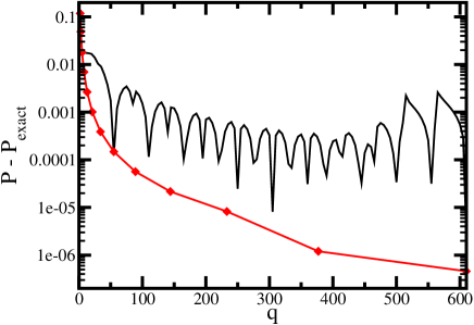
Figure 7: Semilogarithmic plot of the absolute value of the difference between the exact value of the polarization $P_{exact}$ and the polarization calculated via two different methods. The solid like shows the use of an irrational distance (inverse of the golden ratio), the diamonds show a calculation based on a rational approximation to the inverse golden ratio.

Another way of seeing how the fractional polarization arises is to look at the phase variable of the wave function. The wave functions that are the solution of the Hamiltonian in Eq. (7) with the $d$-components given by Eq. (13) can be written in the form

$$\begin{pmatrix}\sin\left(\frac{\theta_{k}}{2}\right)\\ \cos\left(\frac{\theta_{k}}{2}\right)\exp(i\phi_{k})\end{pmatrix},$$ (21)

where $\theta_{k}$ and $\phi_{k}$ depend on $d_{x},d_{y},d_{z}$ (Eq. (13)). The phase $\phi_{k}$ is shown in Fig. 6, for a system with $p=1$ and $q=3$. In the trivial phase, the phase $\phi_{k}$ changes by $2\pi$ as $k$ covers the extended Brillouin zone ($2\pi q=6\pi$). Accordingly, the polarization is $\mathfrak{P}=-\frac{e}{2}\frac{1}{3}$. Meanwhile, in the topological phase, the variable $\phi_{k}$ changes by $-4\pi$ along the Brillouin zone, and the polarization is $\mathfrak{P}=\frac{e}{2}\frac{2}{3}$.

In Fig. 7 we present calculations for an irrational distance, namely the inverse of the golden ratio. In one calculation, we used the irrational number itself to derive a Bloch Hamiltonian (in place of $p/q$ in Eq. (13)), and Brillouin zones of size $-\pi q,\pi q$ were used. In another calculation ratios of the Fibonacci sequence were used to approximate the golden ratio, and Eq. (20) was used. The results in Fig. 7 show that, while the polarization based on using an irrational distance is reasonably close to the exact result, using a rational approximation is a much more stable procedure, which uniformly approaches the exact result.

If an adiabatic charge pumping experiment Atala13 ; Nakajima16 undergoing a full cycle is considered the amount of charge pumped would be one unit of charge per cell. This coincides with the results of Watanabe and Oshikawa Watanabe18 who showed that the charge pumped is independent of how the Hamiltonian is written. Fig. 8a shows the Fourier transform of $Z_{q}$, defined as

$$P_{x}=\sum_{q}\exp(i2\pi xq/L)Z_{q};\hskip 5.69046ptx=1,...,L;$$ (22)

which corresponds to the underlying polarization distribution Souza00 ; Resta99 ; Yahyavi17 ; Hetenyi19 . The case $p/q=1/3$ is considered. Shown are two different parameter sets for each ordered state, as well as the phase transition, where $J=J^{\prime}$. The distributions of the ordered states show maxima corresponding to the values of the polarization calculated above. The tuning of the parameters of the Hamiltonian within one phase change the shape of the distribution (variance and other cumulants), but not the position of the maximum. At the transition the distribution becomes nearly flat, the system does not exhibit a well-defined polarization due to gap closure. For a finite system the curve representing $J=J^{\prime}$ is not entirely flat, because the $k-$space sampling does not precisely hit the points where the gaps occur. However, as the thermodynamic limit is taken, the curve progressively flattens out.

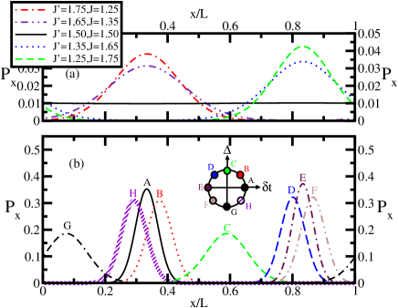
Figure 8: (a) Fourier transform of the polarization amplitude, or polarization distribution shown for different cases of the system with $p/q=1/3$; two sets in each ordered state and at the gap closure point. The curves are normalized to one over the lattice of $L=100$. Legend is valid only for the upper panel. (b) Reconstructed polarization distributions along an adiabatic charge pumping process. For further explanation see the text.

In the cases treated heretofore the polarization can be easily determined by the ratio of the winding numbers, hence the Berry phase formula is not necessary. If other terms are added to the Hamiltonian, for example, an on-site potential, then the Berry phase based formula in Eq. (20) is needed. In the lower panel of Fig. 8b an adiabatic charge pumping process Nakajima16 is shown. The Hamiltonian is reparametrized according to Eq. (10) and an alternating on-site potential of strength $\Delta$ is also added. In the calculations of Fig. 8b $t=K=1$. The plots shown are along total polarization distribution curves along the circle in the $\delta t-\Delta$ plane. The equation of the circle is $0.2\cos(\alpha),0.2\sin(\alpha)$, and the curves labeled $A,B,C,D,E,F,G,H$ correspond to values of $\alpha=0,\pi/4,\pi/2,3\pi/4,\pi,5\pi/4,3\pi/2,7\pi/4$ respectively. As $\alpha$ increases, the maximum of the polarization distribution function shifts towards the right within the unit cell. For the curves $G$ and $H$ the maxima of the curves is to the left of the $A$-curve. This can be interpreted as a charge which entered from a neighboring unit cell (to the left of the one shown), as is expected to occur for adiabatic charge pumping. Note that at points $A$ and $E$ the maxima correspond to the ones shown in Fig. 8a, and the maximum of the charge distribution appears to travel smoothly in between. The part of the adiabatic charge pump process between $\alpha=0$ and $\alpha=\pi$ occurs between systems which exhibit fractionally quantized polarization. If the $I$ basis was used, the maximu would be located at the edge of and halfway through the unit cell.

VI Conclusion

Lattices with a basis can be solved by various representations of the wave function. The representations differ in the relative phases of the Wannier functions associated with different sites within the unit cell. The different representations are related by unitary transformations. The transformation can be used to diagonalize the position operator, if t he Brillouin zone is extended. When the nearest distance between basis sites is a rational number $p/q$, the Brillouin zone has to be extended by a factor of $q$. When this distance is an irrational number, the Brillouin zone extends to the entire real line. This latter state of affairs raises the question of how to calculate the polarization, to which we suggested the use of a rational approximation to the distance between intra-unit cell sites.

Applying such a transformation to the Hamiltonian can give rise to auxiliary topological features. In our example calculations, based on an extension of the SSH model, the $d_{x},d_{y},d_{z}$-curve forms a toroidal knot, and the ratio of the two winding numbers of the torus is proportional to the polarization. Since the modification here is a mere unitary transformation of the Hamiltonian, or a change in the relative phase of the Wannier functions corresponding to the different sites within a unit cell, no new phases are found, the phase diagram is unaltered. If the extended SSH model is studied in the “usual” basis, where the phases of the Wannier functions are the same, then there is no torus, the $d_{x},d_{y},d_{z}$ curve is an ellipse, and its winding number around the $d_{z}$ axis defines the polarization (the distinct phases have winding numbers zero or one). When the Hamiltonian is transformed into the basis which diagonalizes the position, and the Brillouin zone is extended, the $d_{x},d_{y},d_{z}$ curve becomes a knot on a torus. Within each phase the torus on which the “curve” lives is of a different type, a ring or a spindle torus. The quantum phase transition occurs when the torus is a horn torus.

These conclusions fit into the recent findings of Bena and Montambaux Bena09 and those of Watanabe and Oshikawa Watanabe18 . The unitary transformation which relates different representation choices can change quantities which depend on the phase of the wave fuction. In Ref. Watanabe18 this is shown for the current, in our case it is shown for the polarization (Berry-Zak phase), and for the $d_{x},d_{y},d_{z}$ curves of the system. However, as argued in both Ref. Bena09 and Watanabe18 , phase independent quantities Watanabe18 will not change. The phase independent quantity we investigated was the charge pumped in an adiabatic process, and indeed it does not depend on the representation used. The path of the polarization maximum during the process, however, does depend on it.

As for experimental tests of our work, the model suggested here can be realized in a setting of cold atoms trapped in optical lattices Atala13 ; Nakajima16 . We anticipate that a partial change in the polarization, of the type between maxima in Fig. 8 can be measured in experiments in which the polarization is changed, as long as the process does not constitute a full adiabatic cycle, for example, a polarization switch. One possible way to realize the distance dependence explicitly is the following. For instance a $p=1$, $q=3$ system could be realized by constructing first a tri-partite periodic lattice, and approach our bi-partite system as a limit by decreasing the coupling of one of the sites in each unit cell to zero.

References

- (1) C. Bena and G. Montambaux, New J. Phys., 11 095003 (2009).
- (2) H. Watanabe and M. Oshikawa, Phys. Rev. X 8 021065 (2018).
- (3) B. A. Bernevig and T. L. Hughes, Topological Insulators and Superconductors, Princeton University Press (2013).
- (4) C. L. Kane, in Topological Insulators, vol. 6 Eds. M. Franz and L. Molenkamp, Chapter 1, Elsevier (2013).
- (5) J. K. Asbóth, L. Oroszlány, and A. Pályi, A Short Course on Topological Insulators: Band Structure Topology and Edge states in One and Two Dimensions, Lecture Notes in Physics, vol. 919, Springer (2018).
- (6) F. D. M. Haldane, Phys. Rev. Lett. 61 2015 (1988).
- (7) C. L. Kane and E. J. Mele, Phys. Rev. Lett. 95 226801 (2005).
- (8) C. L. Kane and E. J. Mele, Phys. Rev. Lett. 95 146802 (2005).
- (9) W. P. Su, J. R. Schrieffer and A. J. Heeger, Phys. Rev. Lett. 42 1698 (1979).
- (10) D. J. Thouless, M. Kohmoto, M. P. Nightingale and M. den Nijs Phys. Rev. Lett. 49 405 (1982).
- (11) M. V. Berry, Proc. Roy. Soc. London A392 45 (1984).
- (12) J. Zak, Phys. Rev. 62 2747 (1989).
- (13) R. D. King-Smith and D. Vanderbilt, Phys. Rev. B 47 R1651 (1993).
- (14) R. Resta, Phys. Rev. Lett. 80 1800 (1998).
- (15) R. Resta, J. Phys.: Cond. Mat. 12 R107 (2000).
- (16) E. I. Blount, Solid State Physics 13 305 (1962).
- (17) S. Kivelson, Phys. Rev. B 26 4269 (1982).
- (18) N. W. Ashcroft and M. D. Mermin, Solid State Physics (Harcourt, 1976).
- (19) L. Li, Z. Xu, and S. Chen, Phys. Rev. B 89 085111 (2014).
- (20) W. Kohn, Phys. Rev. 133 A171 (1964).
- (21) A. Altland and M. R. Zirnbauer, Phys. Rev. B 55 1142 (1997).
- (22) A. P. Schnyder, S. Ryu, A. Furusaki, A. W. W. Ludwig, Phys. Rev. B 78 195125 (2008).
- (23) R. Jackiw and C. Rebbi, Phys. Rev. D 13 3398 (1976).
- (24) M. Nakahara, Geometry, Topology, and Physics, Graduate Student Series in Physics, CRC Press, 2nd Edition (2003).
- (25) B. Hetényi and B. Dóra, Phys. Rev. B 99 085126 (2019).
- (26) C. C. Adams, The Knot Book, American Mathematical Society, Providence, Rhode Island (2001).
- (27) I. Souza, T. Wilkens, and R. M. Martin, Phys. Rev. B 62 1666 (2000).
- (28) R. Resta and S. Sorella, Phys. Rev. Lett. 82 370 (1999).
- (29) M. Yahyavi and B. Hetényi, Phys. Rev. A 95 062104 (2017).
- (30) M. Atala, M. Aidelsburger, J. T. Barreiro, D. Abanin, T. Kitagawa, E. Demler, I. Bloch, Nat. Phys. 9 795 (2013).
- (31) S. Nakajima, T. Tomita, S. Taie, T. Ichinose, H. Ozawa, L. Wang, M. Troyer, Y. Takahashi, Nat. Phys. 12 296 (2016).