Multi-robot energy autonomy with wind and constrained resources

Abstract

One aspect of the ever-growing need for long term autonomy of multi-robot systems, is ensuring energy sufficiency. In particular, in scenarios where charging facilities are limited, battery-powered robots need to coordinate to share access. In this work we extend previous results by considering robots that carry out a generic mission while sharing a single charging station, while being affected by air drag and wind fields. Our mission-agnostic framework based on control barrier functions (CBFs) ensures energy sufficiency (i.e., maintaining all robots above a certain voltage threshold) and proper coordination (i.e., ensuring mutually exclusive use of the available charging station). Moreover, we investigate the feasibility requirements of the system in relation to individual robots’ properties, as well as air drag and wind effects. We show simulation results that demonstrate the effectiveness of the proposed framework.

I Introduction

The continuous advances in multi-robot systems gave rise to many new applications like patrolling [1], coverage [2], exploration [3] and construction [4] to give a few examples. This has drawn many researchers’ attention in recent years to long term autonomy and resilience of multi-robot systems, with the aim of providing more practical and robust systems.

Energy autonomy, the ability of the robots in a multi-robot system to replenish their energy reserves, is particularly important to extend mission duration and general survivability.

Earlier interest in optimizing energy consumption in a multi-robot system can be traced back to energy aware path planning [5] and node scheduling in wireless sensor networks [6]. These ideas have been applied to multi-robot systems as in [7], where the mission tasks are divided among robots according to their energy content.

One option for tackling the issue of limited energy is through the introduction of stationary or mobile charging stations. Ding et al. [8] propose a method for planning routes of charging robots that deposit batteries along the trajectories of other robots carrying out a surveillance mission. Notomista et al. [9] use a control barrier function framework that allows each robot in a multi-robot system to recharge from a dedicated static charging station in a mission agnostic and minimally invasive manner.

In this work we extend [10], which is in turn inspired from [9], by considering a group of robots affected by air drag that perform a generic mission (e.g. coverage or patrolling) in a known wind field. These robots need to share a single charging station.

The contributions of this paper are: 1) We extend the results in [10] so that the CBF-based coordination framework proposed can account for the effect of air drag and winds, while ensuring mutually exclusive use of the charging station, and 2) we extend the sufficient feasibility conditions proposed in [10] to express the system’s capacity in case of wind and air drag effects and ensure the feasibility of coordination.

II Preliminaries

II-A Control Barrier Functions (CBF)

A control barrier function (CBF)  [11] is a tool that is mainly used to ensure set invariance of control affine systems, having the form

$$\dot{x}=f(x)+g(x)u.$$ (1)

This is often used for ensuring system’s safety by enforcing forward invariance of a desired safe set.

The safe set is defined to be the superlevel set of a continuously differentiable function $h(x)$ such that [11]:

$$\begin{split}\mathcal{C}&=\{x\in\mathbb{R}^{n}:h(x)\geq 0\}\\ \partial\mathcal{C}&=\{x\in\mathbb{R}^{n}:h(x)=0\}\\ Int(\mathcal{C})&=\{x\in\mathbb{R}^{n}:h(x)>0\}\\ \end{split}$$ (2)

where ensuring $h(x)>0,\forall t\geq 0$ implies the safe set $\mathcal{C}$ is positively invariant. For a control affine system, having a control action $u$ that achieves

$$\underbrace{L_{f}h(x)+L_{g}h(x)u}_{\dot{h}(x)}\geq-\alpha(h(x))$$ (3)

where $\alpha(h(x))$ is an extended type $\mathcal{K}$ function, ensures positive invariance of $\mathcal{C}$.

One popular type of CBFs that we use in this paper is the zeroing control barrier function (ZCBF) [12], as they have favourable robustness and asymptotic stability properties [13].

Definition 1

[12] For a region $\mathcal{D}\in\mathcal{C}$ a continuously differentiable function $h(x)$ is called a ZCBF if there exists an extended class $\mathcal{K}$ function $\alpha(h(x))$ such that

$$\sup_{u\in U}\left(L_{f}h(x)+L_{g}hu+\alpha(h(x))\geq 0\right)$$ (4)

The set $K_{zcbf}$[12] is defined as

$$K_{zcbf}=\{u\in U:L_{f}h(x)+L_{g}hu+\alpha(h(x))\geq 0\}$$

and it is the set that contains all the safe control inputs, thus choosing a Lipschitz continuous controller $u\in K_{zcbf}$ ensures forward invariance of $\mathcal{C}$ and system’s safety.

To mix the safety control input with an arbitrary mission’s control input $u_{nom}$, we use a quadratic program:  [9]

$$u^{*}=\underset{u}{\text{min}} ||u-u_{nom}||^{2}$$ (5)

         s.t. $$L_{f}h(x)+L_{g}h(x)u\geq-\alpha(h(x)).$$

II-B Higher order control barrier functions (HOCBF)

If $h(x)$ is of a higher relative degree (the control action $u$ doesn’t appear after differentiating once, i.e. $L_{g}h(x)=0$), using (3) to find an appropriate control action becomes invalid. HOCBFs [14] are an effective solution of this problem. To define a HOCBF, we first need to define the following set of functions for an $m^{th}$ order differentiable function $h(x)$

$$\begin{split}\psi_{0}(x)&=h(x)\\ \psi_{1}(x)&=\dot{\psi}_{0}(x)+\alpha_{1}(\psi_{0}(x))\\ \vdots\\ \psi_{m}(x)&=\dot{\psi}_{m-1}(x)+\alpha_{m}(\psi_{m-1}(x))\end{split}$$ (6)

where $\alpha_{1},\dots,\alpha_{m-1}$ are class $\mathcal{K}$ functions. Also we define the following series of sets

$$\begin{split}\mathcal{C}_{1}\vcentcolon&=\{x\in\mathbb{R}^{n}:\psi_{0}(x)\geq 0\}\\ \vdots\\ \mathcal{C}_{m}\vcentcolon&=\{x\in\mathbb{R}^{n}:\psi_{m}(x)\geq 0\}\end{split}$$ (7)

Definition 2

[14] Let $\mathcal{C}_{1},\mathcal{C}_{2},\dots,\mathcal{C}_{m}$ be defined by (7) and $\psi_{0}(x),\psi_{1}(x),\dots,\psi_{m}(x)$ be defined by (6). A function $h(x)$ is a HOCBF of relative degree $m$ for system (1) if there exists differentiable class $\mathcal{K}$ functions $\alpha_{1},\alpha_{2},\dots,\alpha_{m}$ such that

$$L_{f}^{m}h(x)+L_{g}L_{f}^{m-1}h(x)+O(h(x))+\alpha_{m}(\psi_{m-1}(x))\geq 0$$ (8)

for all $x\in\mathcal{C}_{1}\cap\mathcal{C}_{2}\dots\cap\mathcal{C}_{m}$. Here $O(h(x))$ denotes the remaining Lie derivatives along $f$ with degrees less than or equal $m-1$.

Xiao et al. show in [14, Theorem 5] that choosing a control action that satisfies (8) renders the set $\mathcal{C}_{1}\cap\mathcal{C}_{2}\dots\cap\mathcal{C}_{m}$ forward invariant for system (1).

III Problem formulation

We assume $n$ robots moving in a given wind field with the following dynamics:

$$\begin{split}\dot{\mathbf{x}}&=\mathbf{v}\\ \dot{\mathbf{v}}&=u-C_{d}(\mathbf{v}-\mathbf{v}_{w})\\ \dot{E}&=\begin{cases}-k_{e}-k_{v}||\mathbf{v}-\mathbf{v}_{w}||\quad,\text{if}||\mathbf{x}-\mathbf{x}_{c}||>\delta\\ k_{ch}\quad,\text{Otherwise}\end{cases}\end{split}$$ (9)

where $\mathbf{x}\in\mathbb{R}^{2}$ is the robot’s position, $\mathbf{v}\in\mathbb{R}^{2}$ is its velocity, $C_{d}>0,k_{ch}>0,k_{e}>0,k_{v}>0$ are coefficients of linear drag, recharge, static and dynamic discharge respectively. Also $E>0$ is the robot’s voltage, $u\in\mathbb{R}^{2}$ is the control input (no constraints on the control input), and $\mathbf{v}_{w}$ is a known wind vector. Moreover we suppose that all the robots operate in a certain known operational range $\mathbf{x}\in\mathcal{R}\subset\mathbb{R}^{2}$, where $\mathcal{R}$ is a closed set, and the size of this operational range is described by the operational radius $R_{0}$. The robots are carrying out a mission specified by $u_{nom}$ and they have one charging station at a known location $x_{c}$ (in the origin without loss of generality), and this station can only serve one robot at a time, and has an effective charging range of $\delta>0$.

We point out that in our model we use a linear drag term to account for the air drag effect, which is a reasonable approximation for bodies moving at low speeds. The main assumptions we are adopting in this work are: 1. all robots have the same properties 2. robots have a complete communication graph 3. robots start discharging from the maximum voltage 4. the charging rate is faster than the discharge rate 5. An upper bound of the average relative velocity w.r.t. wind velocity(we call it $\tilde{V}$) of all robots is known at the beginning of the mission. We propose a CBF framework that:

• Ensures no robot runs out of energy during the mission

• Coordinates the times of arrival to the charging station so they are mutually exclusive.

Additionally, we describe the system’s capacity as the relationship between number of robots and robot properties with feasible separation in arrival times at the charging station.

It is worth mentioning that for the rest of the paper we are omitting the proofs due to space constraints, and putting them all in the appendix.

IV Energy sufficiency

We provide a CBF that ensures that the voltage of all robots does not go below a certain desired minimum voltage $E_{min}$. We take inspiration from [9], but we extend it to accommodate the system dynamics in (9). The candidate CBF is

$$h_{e}=E-E_{min}-k_{c}\log\frac{D}{\delta}$$ (10)

where $D=||x-x_{c}||$. The first derivative of this function is

$$\dot{h}_{e}=-k_{e}-k_{v}||\mathbf{v}-\mathbf{v}_{w}||-\frac{k_{v}}{D^{2}}(\mathbf{x}-\mathbf{x}_{c})^{T}\mathbf{v}$$ (11)

so we need to differentiate twice for the control input $u$ to appear

$$\begin{split}&\ddot{h}_{e}=\overbrace{-\left[kv\frac{(\mathbf{v}-\mathbf{v}_{w})^{T}}{||\mathbf{v}-\mathbf{v}_{w}||}+k_{c}\frac{(\mathbf{x}-\mathbf{x}_{c})^{T}}{D^{2}}\right]}^{L_{g}L_{f}h_{e}(x)}u\\ &+k_{v}C_{d}||\mathbf{v}-\mathbf{v}_{w}||\\ &+\frac{k_{c}}{D^{2}}\left[\frac{2((\mathbf{x}-\mathbf{x}_{c})^{T}\mathbf{v})^{2}}{D^{2}}-\mathbf{v}^{T}\mathbf{v}+C_{d}\mathbf{x}-\mathbf{x}_{c})^{T}(\mathbf{v}-\mathbf{v}_{w})\right]\end{split}$$ (12)

with the second and third expressions being $L_{f}^{2}h_{e}(x)$. We can then create an inequality similar to (8) using $\alpha_{1}(h)=p_{1}h$ and $\alpha_{2}(h)=p_{2}h$

$$L_{f}^{2}h_{e}(x)+L_{g}L_{f}h_{e}(x)u+(p_{1}+p_{2})\dot{h}_{e}+p_{1}p_{2}h_{e}\geq 0$$ (13)

and $p_{1}>$ and $p_{2}>$ are chosen in such a way that lends the characteristic equation of the left side of (13) with distinct real roots.

Theorem 1

For a robot described by dynamics in (9), and provided that the robot is out of the charging region, and that $k_{c}>k_{v}R_{0}$, then $h_{e}$ is a HOCBF.

Lemma 1

For a robot with dynamics described by (9) applying a QP as in (5) with (13) as being the constraint, then the quantity $E-E_{min}$ at the time of arrival to the charging station is upper bounded with a quantity exponentially decaying with a rate of $\frac{1}{2}\left(-(p_{1}+p_{2})+|p_{1}-p_{2}|\right)$ and lower bounded by zero.

V Coordination

The second component in our framework ensures that the difference in arrival times of any two robots to the charging station is above a desired limit. The main idea is that if two robots have different values of $E_{min}$, they arrive to the charging station at different times. We propose a method for changing the values of $E_{min}$ to achieve the aforementioned coordination.

To get this expression, we integrate the voltage relation in (9) to get

$$\begin{split}\int_{E_{max}}^{E_{min}}\dot{E}dt&=-\int_{0}^{T_{L}}(k_{e}+k_{v}||\mathbf{v}-\mathbf{v}_{w}||)dt\\ E_{max}-E_{min}&=k_{e}T_{L}+k_{v}\int_{0}^{T_{L}}||\mathbf{v}-\mathbf{v}_{w}||dt.\end{split}$$ (14)

Supposing we have the average relative speed $\bar{z}=\frac{1}{T_{L}}\int_{0}^{T_{L}}||\mathbf{v}-\mathbf{v}_{w}||dt$, the last integral can be replaced and the arrival time becomes

$$T_{L}=\frac{E_{max}-E_{min}}{k_{e}+k_{v}\bar{z}}.$$ (15)

We then replace $E_{max}$ in the last expression by $E(t)$ to get an expression for $T_{L}(t)$ that changes with time

$$T_{L}(t)=\frac{E(t)-E_{min}}{k_{e}+k_{v}\bar{z}}.$$ (16)

In this work, we use a moving average $\bar{V}$ to estimate the average velocity relative to wind defined as

$$\bar{V}=\frac{1}{w}\int_{0}^{w}||\mathbf{v}-\mathbf{v}_{w}||dt$$ (17)

where $w>0$ is the width of the integration window. The larger the window, the closer the estimate is to the true average. The approximate value of the arrival time is

$$T_{L}(t)\approx\frac{E(t)-E_{min}}{k_{e}+k_{v}\bar{V}}.$$ (18)

To be able to change $E_{min}$ to achieve coordination, we propose a simple single integrator model for $E_{min}$ as follows

$$\dot{E}_{min}=\eta$$ (19)

where $\eta\in\Theta\subset\mathbb{R}$ is a control input to manipulate $E_{min}$,and $\Theta$ is being the set of all possible values of $\eta$. It is useful to point out that $\eta$ has a default value of $\eta_{nom}=0$ unless modified by the proposed coordination framework.

V-A Coordination CBF

We propose a CBF approach to change the values of $E_{min}$ to ensure mutually exclusive use of the charging station. We define a coordination CBF $h_{c_{ij}}$ between robots $i$ and $j$, as well as an associated pairwise safe set $\mathcal{C}_{ij}$

$$\mathcal{C}_{ij}=\{(E_{min_{i}},E_{min_{j}})\in\mathbb{R}^{2}:h_{c_{ij}}\geq 0\}.$$ (20)

We use the same coordination CBF as in [10]

$$h_{c_{ij}}=\log\frac{|T_{L_{i}}-T_{L_{j}}|}{\delta_{t}}$$ (21)

and to get a constraint similar to (3)

$$\frac{T_{L_{i}}-T_{L_{j}}}{|T_{L_{i}}-T_{L_{j}}|^{2}}(\theta_{i}\eta_{i}+\beta_{i}-\beta_{j})\geq\alpha(h_{c_{ij}})$$ (22)

where

$$\begin{split}&\theta_{i}=-\frac{1}{k_{e}+k_{v}\bar{V}}\\ &\beta_{i}=\frac{-k_{e}-k_{v}V}{k_{e}+k_{v}\bar{V}}-\frac{k_{v}}{w}\frac{(E-E_{min})(V(t)-V(t-w))}{k_{e}+k_{v}\bar{V}}\\ &\dot{T}_{L_{i}}=\theta_{i}\eta_{i}+\beta_{i}\end{split}$$

where $V=||\mathbf{v}-\mathbf{v}_{w}||$. For decentralized implementation, we dropped out the term $\theta_{j}$ so the constraint equation is independent of $\eta_{j}$, and provided both robots are adopting the constraint (22), each will try to stay in the safe set $\mathcal{C}_{ij}$. For the right hand side of (22) we use the following

$$\begin{split}&\alpha(h_{c_{ij}})=\gamma_{ij}.\text{sign}(h_{c_{ij}}).|h_{c_{ij}}|^{\rho}\quad,\rho\in\left[0,1\right)\\ &\gamma_{ij}=\begin{cases}\gamma_{h}\quad,\text{if}\hskip 5.69054ptD_{i}>\delta\text{ and }D_{j}>\delta\\ 0\quad,\text{otherwise}\end{cases}\end{split}$$ (23)

which is inspired from [15] and leads to the favourable quality of converging to the safe set in a finite time, in case the initial condition is out of the safe set.

Theorem 2

[10, Theorem 2] For a pair of robots $(i,j)$ that belongs to a multi-robot system and satisfying $D_{i}>\delta$ and $D_{j}>\delta$, and provided that $\eta\in\Theta=\mathbb{R}$ then $h_{c_{ij}}$ is a ZCBF. Moreover, if $(E_{min_{i}}(t_{0}),E_{min_{j}}(t_{0}))\notin\mathcal{C}_{ij}$, then the constraint (22) leads $(E_{min_{i}}(t),E_{min_{j}}(t))$ to converge to $\partial\mathcal{C}_{ij}$ in finite time.

V-B Lower bound on $E_{min}$

Since $E_{min}$ is supposed to be the voltage at which the robot arrives to the charging station, then it is necessary to enforce a lower bound on its value to avoid any potential damage to the batteries or the loss of a robot with excessively low voltage. For this reason, we propose another CBF:

$$h_{L}=k_{s}(E_{min}-E_{lb})$$ (24)

where $E_{lb}>0$ is the desired lower bound voltage and $k_{s}>0$ is a scaling gain. Differentiating $h_{L}$ and obtaining the QP constraint gives

$$k_{s}\eta\geq-\alpha(h_{L})$$ (25)

where $\alpha(h_{L})=p_{L}h_{L}$ for $p_{L}>0$. It can be easily shown that $h_{L}$ is a ZCBF, since $\eta\in\Theta=\mathbb{R}$ (no constraint on $\eta$) then there exists a control input $\eta$ that satisfies (25).

V-C System capacity description

To successfully apply the coordination CBF in a pairwise manner, the value of the desired $\delta_{t}$ should be reasonable with respect to individual robot’s properties and the number of robots in the system (e.g. we can’t ask for $\delta_{t}$ that is longer than the total discharge time of a battery). We consider the relation between the robots’ parameters, their number and the feasible limits on $\delta_{t}$ as being an expression of the system’s capacity.

We propose a sufficient condition on the upper and lower limits of $\delta_{t}$, in relation to properties like maximum and minimum battery voltages, discharge and recharge rates, and the number of robots in the system.

Figure 1: Schematic of a charging cycle with three robots. The red line represents the more needy robot, while the blue one is the least needy one, and it defines one recharging cycle.

For the sake of being conservative, we derive this capacity relation assuming that the system is pushed to its limits, meaning that all robots operate with the maximum average relative velocity w.r.t. wind $\tilde{V}$. Suppose we have a group of $n$ robots, each has its own $E_{min}$ value, and one of them is the “neediest” robot that recharges first and most often, while another is the least needy one (represented in Figure 1 as the red and blue lines respectively). We want $t_{2}-t_{1}\geq\delta_{t}$, which means

$$\begin{split}&t_{1}=\frac{E_{max}-E_{lb}}{k_{e}+k_{v}\tilde{V}}\\ &t_{2}=\frac{E_{max}-\bar{E}_{M}}{k_{e}+k_{v}\tilde{V}}+\frac{E_{max}-\bar{E}_{M}}{k_{ch}}+\frac{E_{max}-\bar{E}_{M}}{k_{e}+k_{v}\tilde{V}}.\end{split}$$ (26)

Calculating $t_{2}-t_{1}$ and considering that $\bar{E}_{M}=E_{M}+\varepsilon$, where $E_{M}$ being the actual value of $E_{min}$ of the neediest robot during the coordination, and $\varepsilon\geq 0$ being an additional increment of voltage to $E_{M}$ that is caused by the dependence of discharge rate on robot’s speed, we have:

$$E_{M}\leq\frac{(1+\tfrac{k_{e}+k_{v}\tilde{V}}{k_{ch}})E_{max}+E_{lb}-\delta_{t}(k_{e}+k_{v}\tilde{V})-\kappa\varepsilon}{\kappa}$$ (27)

where $\kappa=2+\tfrac{k_{e}+k_{v}\tilde{V}}{k_{ch}}$. We can then calculate $\Delta E_{M}=\tfrac{E_{M}-E_{lb}}{n-1}$ which is a uniform increment of $E_{min}$ between $E_{lb}$ and $E_{M}$ to create the desired separation of arrival times

$$\Delta E_{M}=\frac{(1+\tfrac{k_{e}+k_{v}\tilde{V}}{k_{ch}})(E_{max}-E_{lb})-\delta_{t}(k_{e}+k_{v}\tilde{V})-\kappa\varepsilon}{\kappa(n-1)}$$ (28)

What we want then is to have $t_{1}-t_{3}\geq\delta_{t}$, meaning that the arrival times of the last two robots (or any two consecutive robots) to be at least $\delta_{t}$

$$\frac{E_{max}-E_{lb}}{k_{e}+k_{v}\tilde{V}}-\frac{E_{max}-(E_{lb}+\Delta E_{M})}{k_{e}+k_{v}\tilde{V}}\geq\delta_{t}$$ (29)

and substituting 28 into the last equation we get

$$\begin{split}&\frac{(1+\tfrac{k_{e}+k_{v}\tilde{V}}{k_{ch}})(E_{max}-E_{lb})-\delta_{t}(k_{e}+k_{v}\tilde{V})-\kappa\varepsilon}{\kappa(n-1)}\\ &-\delta_{t}(k_{e}+k_{v}\tilde{V})\geq 0\end{split}$$ (30)

then we obtain a critical value of $\delta_{t}$ at which the inequality becomes an equality

$$\delta_{t_{cr}}=\frac{\left(1+\frac{k_{e}+k_{v}\tilde{V}}{k_{ch}}\right)(E_{max}-E_{lb})-\kappa\varepsilon}{(k_{e}+k_{v}\tilde{V})\left[1+\kappa(n-1)\right]}.$$ (31)

One final requirement on $\delta_{t_{cr}}$ is to be greater than half the time taken to recharge a battery from $E_{lb}$ to $E_{max}$

$$\delta_{t_{cr}}\geq\frac{E_{max}-E_{lb}}{2k_{ch}}$$ (32)

The value of $\delta_{t_{cr}}$ represents in this case an upper bound on the feasible $\delta_{t}$ that can be achieved by the system. To motivate the need for $\varepsilon$, we consider the critical case when $(E_{min_{i}},E_{min_{j}})\notin\mathcal{C}_{ij}$, in which case the QP produces $\eta_{i}$ that renders (22) an equality, thus $\dot{h}_{c_{ij}}=\alpha(h_{c_{ij}})$ that reaches steady state in finite time (i.e. coordination achieved) at which $\dot{h}_{c_{ij}}=0$. Considering the case where all robots have same $\bar{V}=\tilde{V}$ (which we already supposed when deriving $\delta_{t_{cr}}$) then from the LHS of (22) we have $\eta_{i}=k_{v}(V_{j}-V_{i})$. So if $V_{i}$ decreases (robot $i$ going to recharge for example), $\eta_{i}$ increases and so $\varepsilon=\Delta E_{min_{i}}$ resulting from the increase in $\eta$. The value of $\varepsilon$ can be estimated by approximating the integration of $\eta_{i}$ over the time it takes the robot to go back to the charging station. One approximation for $\varepsilon$ is

$$\varepsilon=\frac{k_{v}V_{n}\left(T_{end}-\tfrac{n(E_{max}-E_{lb})-k_{c}\log\tfrac{R_{0}}{\delta}(1+\kappa(n-1))}{(k_{e}+k_{v}\tilde{V})(1+\kappa(n-1))}\right)}{1+\tfrac{k_{v}V_{n}}{k_{e}+k_{v}\tilde{V}}\left(1-\tfrac{1}{1+\kappa(n-1)}\right)}$$ (33)

where $T_{end}=\frac{E_{max}-\tfrac{E_{max}+E_{lb}}{2}}{k_{e}+k_{v}\tilde{V}}$, and $V_{n}$ is the magnitude of the mission’s nominal velocity w.r.t. the wind velocity vector.

Lemma 2

For a group of $n$ robots that have distinct values of $E_{min}$ that satisfy (31), (32) and (28), and provided they all operate such that their average relative velocity (w.r.t. wind) is equal to its upper bound, i.e. $\bar{V}=\tilde{V}$, let $z_{i}$ be the number of recharges that one robot can have in one charging cycle, then the maximum number of recharges for any robot is $\bar{z}_{i}=2$. Moreover, $\bar{E}_{M}\leq\tfrac{E_{max}+E_{lb}}{2}$.

Lemma 3

For a group of $n$ robots, if $\delta_{t}$ satisfies

$$\frac{E_{max}-E_{lb}}{2k_{ch}}\leq\delta_{t}\leq\delta_{t_{cr}}$$ (34)

as well as equation (28), then there exists $\mathbf{E}_{m}=\{E_{min_{1}},\dots,E_{min_{n}}\}$ such that the difference in arrival times between any two robots is at least $\delta_{t}$ (i.e. the scheduling problem is feasible).

V-D Feasibility of QP

In the proposed coordination framework so far $E_{min}$, which is a 1-D value, is being manipulated to vary the arrival times of robots to the charging station. However, this can potentially cause a QP infeasibility problem. For example, a robot might need to use a negative $\eta$ to evade a neighbour’s arrival time, but at the same time it may need $\eta$ to be positive so as not to go below $E_{lb}$. Some methods have been proposed to deal with this issue as in  [16] and [17], and we adapt the core idea of the latter. To avoid the infeasibility problem, each agent carries out coordination only with its neighbour with the closest arrival time. Moreover, it gives higher priority for maintaining $E_{min}\geq E_{lb}$ over coordination. This way $\eta$ has to change to adapt one thing at a time and avoid potential infeasibility (see Algorithm 1).

Input: $T_{L_{k}}\quad,\forall k\in\mathcal{N}_{i}$

Result: $A_{c}$ and $B_{c}$ for QP constraints

$h_{c_{min}}=h_{0}$

$h_{L_{i}}=E_{min_{i}}-E_{lb}$

while j in $\mathcal{N}_{i}$ do

       $h_{c_{ij}}=\log\tfrac{T_{L_{i}}-T_{L_{j}}}{\delta}$

      if $h_{c_{ij}}<h_{c_{min}}$ and $D_{j}>\delta$ then

             $h_{c_{min}}=h_{c_{ij}}$

       end if

      

end while

if $h_{c_{min}}<h_{L_{i}}$ then

       $A_{c}=L_{g}h_{c_{min}}$

      $B_{c}=-L_{f}h_{c_{min}}-\alpha(h_{c_{min}})$ …(eqn. 22)

else

       $A_{c}=L_{g}h_{L_{i}}$

      $B_{c}=-L_{f}h_{L_{i}}-\alpha(h_{L_{i}})$ …(eqn. 25)

end if

Algorithm 1 Coordination algorithm

The final QP is

$$\mathbf{u}^{*}=\underset{\mathbf{u}\in\mathbb{R}^{3}}{\text{min}} ||\mathbf{u}-\mathbf{u}_{nom}||^{2}$$ (35)

         s.t. $$A\mathbf{u}\geq B$$

where

$$\begin{split}A&=\begin{bmatrix}A_{e}^{T}\\ A_{c}^{T}\end{bmatrix}=\begin{bmatrix}L_{g}L_{f}h_{e}&0\\ \mathbf{0}_{1\times 2}&A_{c}^{T}\end{bmatrix},\\ B&=\begin{bmatrix}B_{e}\\ B_{c}\end{bmatrix}=\begin{bmatrix}-L_{f}^{2}h_{e}-(p_{1}+p_{2})\dot{h}_{e}-p_{1}p_{2}h_{e}\\ B_{c}\end{bmatrix}\end{split}$$

while $A_{c}$ and $B_{c}$ are determined from Algorithm (1).

Theorem 3

[10, Theorem 3] For a multi robot system of $n$ robots, with dynamics defined in (9), and each robot applying energy sufficiency, coordination and lower bound constraints defined in (13), (22) and (25), and provided that the inequalities (27) and (34) are satisfied, then Algorithm (1) ensures mutual exclusive use of the charging station.

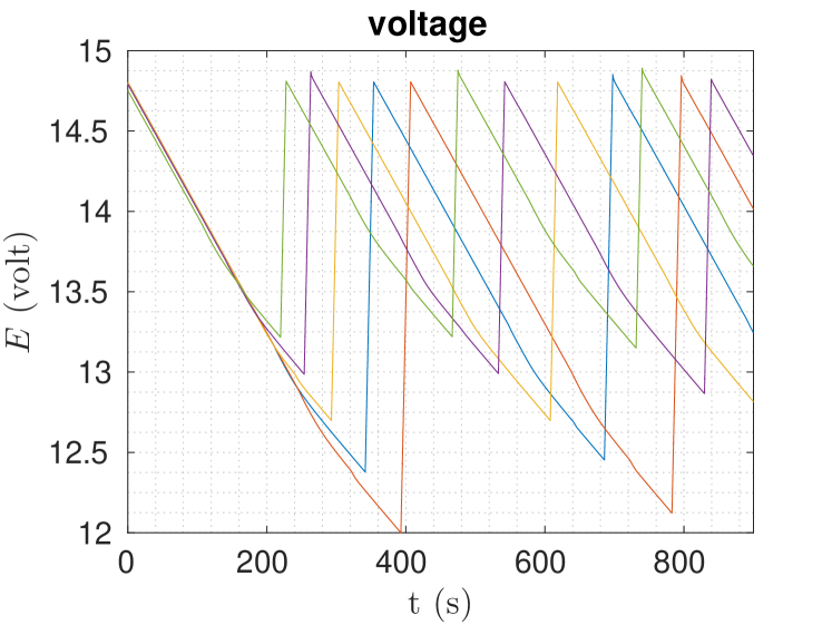
(a)

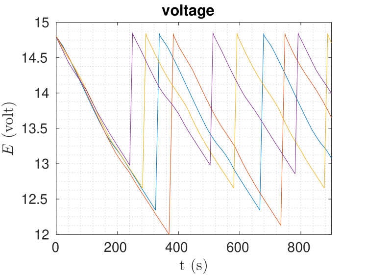
(b)

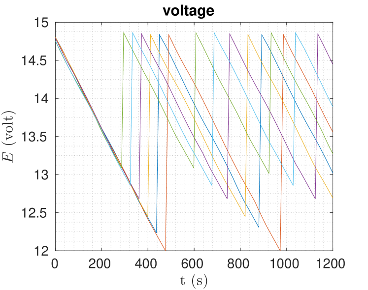
(c)

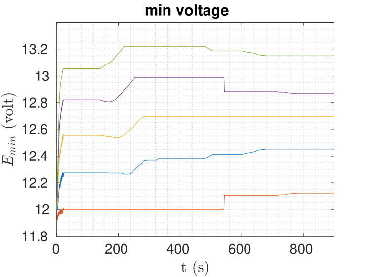
(d)

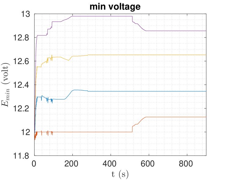
(e)

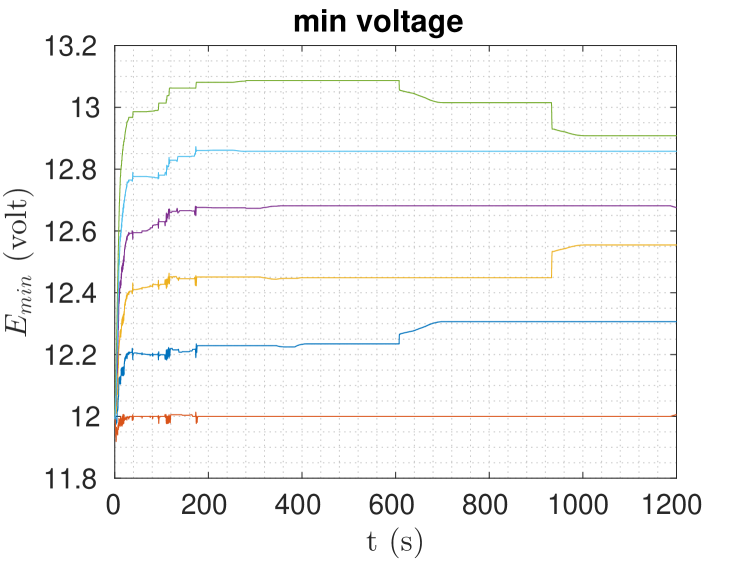
(f)

Figure 2: Evolution of values of $E(t)$ and $E_{min}(t)$ for the three different scenarios under consideration

VI Results

In this section we present Matlab simulation results of the proposed framework, aiming to highlight its effectiveness, as well as the utility of the capacity estimation we propose. We tackled three different scenarios of a simple patrolling mission for a group of robots spinning around the charging station at a certain distance with a desired nominal mission speed. In these scenarios we have $\delta=0.2$\mathrm{m}$$, $R_{0}=9$\mathrm{m}$$ and we want to achieve $\delta_{t}=35$\mathrm{s}$$. The results are depicted in Figure 2, and the main parameters used are presented in Table I. For all the cases discussed, the $\varepsilon$ is calculated using (33).

TABLE I: Values of parameters used in simulation

Parameter	$k_{e}$	$k_{v}$	$k_{ch}$	$E_{max}$	$E_{lb}$
Value	0.005$\mathrm{V}\mathrm{/}\mathrm{s}$	0.015$\mathrm{V}\mathrm{/}\mathrm{m}$	0.2$\mathrm{V}\mathrm{/}\mathrm{s}$	14.8$\mathrm{V}$	12$\mathrm{V}$

VI-A Base scenario

In this scenario we have a group of five robots that revolve around the charging station, with an upper bound of average relative velocity $\tilde{V}=0.15$\mathrm{m}\mathrm{/}\mathrm{s}$$.

Each robot applies a proportional control on the speed to produce a nominal control input $u_{nom}=-k_{d}(\mathbf{v}-\mathbf{v}_{n})$, where $\mathbf{v}_{n}$ is a nominal mission velocity and $k_{d}>0$ is a gain. The value of $u_{nom}$ is the one that goes into the QP (35). To generate $\mathbf{v}_{n}$ for patrolling, we specify a desired magnitude $V_{n}=||\mathbf{v}_{n}||$ then we use potential flow theory to specify the direction. We calculate a potential function $\phi$ of a source near the charging station, and of a vortex near the boundary

$$\phi=\begin{cases}m\log D\quad,\text{if }\hskip 2.84544ptD<\delta+\Delta_{tol}\\ \frac{m}{2\pi}\theta_{p},\text{if }\hskip 2.84544ptD>R_{0}+\Delta_{tol}\end{cases}$$ (36)

where $m>0$, $\Delta_{tol}>0$, $\theta_{p}=\angle(\mathbf{x}-\mathbf{x}_{c})$ and $\mathbf{v}_{n}=V_{n}\tfrac{\nabla\phi}{||\nabla\phi||}$.

The requirement is to have a $\delta_{t}=35$\mathrm{s}$$. The value of $\delta_{t_{cr}}$ from (31) is $\delta_{t_{cr}}=36.39$\mathrm{s}$$ for $\varepsilon=0.24$, and $\tfrac{E_{max}-E_{lb}}{2k_{ch}}=7$\mathrm{V}$$, thus (34) is satisfied. The evolution of voltages and $E_{min}$ values is depicted in figures 2(a) and 2(d).

VI-B Base scenario with wind

Here we add a constant wind field of $\mathbf{v}_{w}=(0.08,0.08)$\mathrm{m}\mathrm{/}\mathrm{s}$$ and we have an upper bound $\tilde{V}=0.2$\mathrm{m}\mathrm{/}\mathrm{s}$$. In this case $\delta_{t_{cr}}=31.9$\mathrm{s}$<\delta_{t}$ for $\varepsilon=0.28$. Choosing to use 5 robots causes $E_{min}$ for some robots to go over $\tfrac{E_{max}+E_{lb}}{2}$ as shown in Figure 3 (when it should be less if it abides by the capacity condition (34), according to lemma 2), which is a sign of overloading the system. Reducing the robots to 4 gives $\delta_{t_{cr}}=41.1$\mathrm{s}$>\delta_{t}$ for $\varepsilon=0.27$. $E(t)$ and $E_{min}(t)$ are depicted in Figs. 2(b) and 2(e).

VI-C Base scenario with wind and less $k_{v}$

Here we consider the same previous scenario, but with robots having $k_{v}=0.0045$. Here for 5 robots $\delta_{t_{cr}}=48.3$\mathrm{s}$$ for $\varepsilon=0.14$, which alludes to the possibility of adding a robot. Indeed, for 6 robots $\delta_{t_{cr}}=39.5$\mathrm{s}$>\delta_{t}$ for $\varepsilon=0.14$. $E(t)$ and $E_{min}(t)$ are depicted in figures 2(c) and 2(f).

Figure 3: Plot of $E_{min}$ when (34) is not satisfied, as described in the second scenario.

VII Conclusions

In this paper we propose a CBF based framework for ensuring energy sufficiency of a multi-robot system while sharing one charging station in a mutually exclusive manner, given that the robots are affected by air drag and known constant wind fields.

As a future work we consider extending the current framework to allow for sharing multiple charging stations, as well as exploring the possibility of relaxing the assumption of having complete communication graph.

Appendix A Proof of theorem 1

Proof:

Since $u\in\mathbb{R}^{2}$ then there should be a value of control input that satisfies (13) provided that $L_{g}L_{f}h(x)\neq 0$. $L_{g}L_{f}h(x)$ can be written as

$$L_{g}L_{f}h(x)=-kv\frac{(\mathbf{v}-\mathbf{v}_{w})^{T}}{||\mathbf{v}-\mathbf{v}_{w}||}-\frac{k_{c}}{D}\frac{(\mathbf{x}-\mathbf{x}_{c})^{T}}{D}$$ (37)

both expressions are basically unit vectors multiplied by an expression or a factor. If we want the second expression to dominate the first one (so even if both vectors are opposite, the summation will not be equal to zero), we pick $k_{c}$ so that the least possible value of $\frac{k_{c}}{D}$ be greater than $k_{v}$ so $\frac{k_{c}}{R_{0}}>k_{v}\Rightarrow k_{c}>R_{0}k_{v}$, meaning $L_{g}L_{f}h(x)\neq 0$. ∎

Appendix B Proof of lemma 1

Proof:

To show this, it is useful to point out to the fact that the minimum value of the quadratic cost function of the QP (5) would be $u=u_{nom}$ in case $u_{nom}$ doesn’t violate the constraints on the QP. Otherwise, the QP produces a value of $u$ that abides with the constraint in the equality sense (produces a control input that renders the constraint as an equality).

Provided that the system starts in the safe set for $h_{e}>0$, then at some time $T_{b}$ the nominal control action will cause inequality (13) to be violated, in which case the QP produces a safe control input $u$ that follows the constraint in the sense of equality. Therefore the produced control input causes $h_{e}$ to vary in the following way

$$\ddot{h}_{e}+(p_{1}+p_{2})\dot{h}_{e}+p_{1}p_{2}h_{e}=0$$ (38)

for which the solution is

$$h(t)=Ae^{\lambda_{1}t}+Be^{\lambda_{2}t}$$ (39)

where $\lambda_{1}=\frac{1}{2}\left(-(p_{1}+p_{2})+|p_{1}-p_{2}|\right)$ (the dominant mode),$\lambda_{2}=\frac{1}{2}\left(-(p_{1}+p_{2})-|p_{1}-p_{2}|\right)$, and the constants $A$ and $B$ are determined from the initial conditions on $h_{e}$ and $\dot{h}_{e}$ at the time $T_{b}$.

When the robot arrives on the boundary of the charging station at time $t_{a}$ we have

$$h_{e}(t_{a})=E(t_{a})-E_{min}=Ae^{\lambda_{1}t_{a}}+Be^{\lambda_{2}t_{a}}$$ (40)

thus by properly choosing $p_{1}$ and $p_{2}$ we can gauge how closely the robot tracks $E_{min}$ on arrival to the charging station. We also point out to the fact that $h_{e}=0$ only at the boundary of the charging region, because if $E=E_{min}$ (which is the boundary of our safe set so to speak) we want this to be at $h_{e}=0$, which happens if $\log\frac{D}{\delta}=0\Rightarrow D=\delta$.

Since $h_{e}$ is a HOCBF, then any control input satisfying (13) renders the safe set forward invariant ($h_{e}\geq 0$) so in case if $h_{e}=0$ and being on the boundary at the same time, then $E-E_{min}=0$. ∎

Appendix C A method for choosing $k_{c}$

In this discussion we provide a heuristic to choose the value of $k_{c}$ in the definition of the energy sufficiency CBF. The third term in the definition of $h_{e}$ signifies the voltage change that a robot needs to go back to the charging station [9]. The basic idea of choosing $k_{c}$ starts by supposing that a robot can use a PD controller to go back to the charging station, starting on the boundary of the operating range (i.e. $||\mathbf{x}_{0}||=R_{0}$). For more conservatism, we suppose that there is a headwind with a magnitude of $||\mathbf{v}_{w}||$ opposing the robot’s motion. Without loss of generality, we suppose that the robot is moving on a line so the robot’s motion is 1-D, and that the charging station is in the origin. In this case the system’s model will be

$$\begin{split}\dot{x}&=v\\ \dot{v}&=-k_{p}x-k_{d}v-C_{d}(v-||\mathbf{v}_{w}||)\\ \end{split}$$ (41)

which is a second order ordinary differential equation, the solution of which is

$$\begin{split}x(t)&=\frac{R_{0}}{G}\left[\left(L_{2}-c\right)e^{-L_{2}t}-\left(L_{1}-c\right)e^{-L_{1}t}\right]\\ &+\frac{C_{d}||\mathbf{v}_{w}||}{Gk_{p}}\left[L_{1}\left(e^{-L_{2}t}-1\right)-L_{2}\left(e^{-L_{1}t}-1\right)\right]\\ v(t)&=\frac{C_{d}||\mathbf{v}_{w}||-R_{0}k_{p}}{D}\left(e^{-L_{1}t}-e^{-L_{2}t}\right)\end{split}$$ (42)

where $c=k_{d}+C_{d}$, $G=\sqrt{c^{2}-4k_{p}}$,$L_{1}=\frac{c-G}{2}$,$L_{2}=\frac{c+G}{2}$. We then approximate the time needed to go from the initial position to a distance $\delta$ from the center (arriving at the boundary of the charging region) by taking only the dominant terms in consideration, so the position equation will be

$$x(t)=\left(\frac{R_{0}}{G}(c-L_{1})-\frac{C_{d}||\mathbf{v}_{w}||}{Gk_{p}}L_{2}\right)e^{-L_{1}t}+\frac{C_{d}||\mathbf{v}_{w}||}{Gk_{p}}L_{2}$$ (43)

thus the time at which $x(t)=\delta$ is

$$\Delta T=\frac{1}{L_{1}}\log\left(\frac{-C_{d}||\mathbf{v}_{w}||L_{2}+(c-L_{1})k_{p}R_{0}}{-C_{d}||\mathbf{v}_{w}||L_{2}+k_{p}G\delta}\right)$$ (44)

then in order to consider the voltage change during this trip back to the charging station, we can integrate the voltage rate $\dot{E}=-k_{e}-k_{v}||v-v_{w}||$, however, to increase the conservatism in the estimate we choose to consider that the robot is moving on a constant speed equal to the maximum peak speed of $v(t)$, which can be obtained by differentiating $v(t)$ and getting the time at which the differential is equal to zero and use the velocity at this time, and we call it $v^{*}$ which is expressed as

$$v^{*}=\frac{-R_{0}k_{p}+C_{d}||\mathbf{v}_{w}||}{G}\left(\left(\frac{L_{2}}{L_{1}}\right)^{\frac{-L_{2}}{L_{2}-L_{1}}}-\left(\frac{L_{2}}{L_{1}}\right)^{\frac{-L_{1}}{L_{2}-L_{1}}}\right)$$ (45)

and the voltage change needed becomes

$$\begin{split}&\Delta E=\dot{E}\Delta T\\ &=-\underbrace{\frac{k_{e}+k_{v}(|v^{*}|+||\mathbf{v}_{w}||)}{L_{1}}}_{k_{c}}\log\left(\frac{-C_{d}||\mathbf{v}_{w}||+(c-L_{1})k_{p}GR_{0}}{-C_{d}||\mathbf{v}_{w}||+k_{p}G\delta}\right)\end{split}$$ (46)

however the current form of $\Delta E$ does not necessarily satisfy the condition that $E=E_{min}$ only on the boundary of the charging region, so we choose

$$\Delta E=-k_{c}\log\left(\frac{D}{\delta}\right)$$ (47)

Appendix D Proof of Theorem 2

Proof:

Since $\eta\in\Theta=\mathbb{R}$ there exists a control action $\eta$ that satisfies (22)) (and keeps $\mathcal{C}_{ij}$ invariant), then to show that $h_{c_{ij}}$ is a ZCBF, we need to ensure that $|T_{L_{i}}-T_{L_{j}}|\neq 0$.

The only chance that this difference can be equal to zero is when one of the robots enters to the charging region. To show this, consider having two robots $(i,j)$ applying (22)and without loss of generality suppose that robot $j$ arrives at the charging station, so the difference in arrival times is

$$\Delta T_{L_{ij}}=\frac{E_{i}-E_{min_{i}}}{k_{e}+k_{v}\bar{V}_{i}}-\frac{E_{j}-E_{min_{j}}}{k_{e}+k_{v}\bar{V}_{j}}>0$$ (48)

it suffices to show that by the end of the charging process $\Delta T_{ij}<0$ which means that $\Delta T_{ij}=0$ at some point. To show this, we first point out that when the QP manipulates $\eta$ for coordination, then (22) becomes an equality, and due to the choice of $\gamma$ in (23), the right hand side will be equal to zero. Thus

$$\eta_{i}\approx-(k_{e}+k_{v}\bar{V}_{i})\left(-\frac{k_{e}+k_{v}V_{j}}{k_{e}+k_{v}\bar{V}_{j}}+\frac{k_{e}+k_{v}V_{i}}{k_{e}+k_{v}\bar{V}_{i}}\right)$$ (49)

notice that we neglected the expression $\frac{k_{v}}{w}\frac{(E-E_{min})(V(t)-V(t-w))}{k_{e}+k_{v}\bar{V}}$ because it can be significantly less than $\frac{k_{e}+k_{v}V_{i}}{k_{e}+k_{v}\bar{V}_{i}}$ for most cases of $w$. An extreme case for (49) can be anticipated if we neglect $\frac{k_{e}+k_{v}V_{j}}{k_{e}+k_{v}\bar{V}_{j}}$ alltogether and take $V_{i}=\max(V_{n},\tilde{V})$, so an extreme case for $\eta_{i}$ can be

$$\eta_{i}\approx-(k_{e}+k_{v}\max\{V_{n},\tilde{V}\})$$ (50)

however if $|\eta_{i}|$ is less than $k_{ch}$ (by assumption) it means that $E_{j}$ increases faster than $E_{min}$ changes for both robots $(i,j)$ (noticing that for $\eta_{j}$ the bracket in (49) will be of reversed sign). Without loss of generality, for cases where $k_{ch}\gg(k_{e}+k_{v}\max\{V_{n},\tilde{V}\})$ we can consider the change in $E_{min}$ values is sufficiently slow that they can be considered constant, so from (48) the value of $T_{L_{j}}$ is increasing in a faster rate than $T_{L_{i}}$ is decreasing, and at some point $T_{L_{j}}=\frac{E_{max}-E_{min_{j}}}{k_{e}+k_{v}\bar{V}_{j}}>\frac{E_{i}-E{min_{i}}}{k_{e}+k_{v}\bar{V}_{i}}=T_{L_{i}}$, which means that $\Delta T_{L_{ij}}=0$ at some point during the recharge.

The proof of the second part is the same as that of proposition III.1 in [15] and is omitted for brevity. ∎

Remark 1

To demonstrate the fact that $k_{ch}$ is sufficiently big, a minimum threshold on $k_{ch}$ can be obtained by equating $\delta_{t_{cr}}$ with $\frac{E_{max}-E_{lb}}{2}$ in (34). In other words, by doing so we can get a minimum acceptable value of $k_{ch}$ so that the capacity constraint (34) is technically satisfied. Doing so we get

$$k_{ch}=(k_{e}+k_{v}\tilde{V})\left[\tfrac{(2(n-1)\Delta E+\varepsilon)\pm\sqrt{(2(n-1)\Delta E+\varepsilon)^{2}+4(n-1)(\Delta E-2\varepsilon)\Delta E}}{2(\Delta E-2\varepsilon)}\right]$$ (51)

where $\Delta E=E_{max}-E_{lb}$. If we set $\varepsilon=0$ for simplicity, and for $n=2$ we get $k_{ch}=(1+\sqrt{2})(k_{e}+k_{v}\tilde{V})$. In practice, the value of $\delta_{t_{cr}}$ is usually significantly larger than $\frac{E_{max}-E_{lb}}{2k_{ch}}$. Moreover the value of $n$ is bigger than two, which means that $k_{ch}$ is in practice significantly larger than $(k_{e}+k_{v}\tilde{V})$.

Appendix E Proof of lemma 2

Proof:

We start by showing that

$$\bar{E}_{M}\leq\frac{E_{max}+E_{lb}}{2}$$

To do this, we calculate the difference

$$\begin{split}&\tfrac{E_{max}+E_{lb}}{2}-\bar{E}_{M}=\tfrac{E_{max}+E_{lb}}{2}-\tfrac{(1+\tfrac{k_{e}+k_{v}\tilde{V}}{k_{ch}})E_{max}+E_{lb}-\delta_{t}(k_{e}+k_{v}\tilde{V})}{\kappa}\end{split}$$ (52)

where $\kappa=2+\tfrac{k_{e}+k_{v}\tilde{V}}{k_{ch}}$. This gives

$$\tfrac{E_{max}+E_{lb}}{2}-\bar{E}_{M}=\tfrac{(k_{e}+k_{v}\tilde{V})}{2\kappa}\left(2\delta_{t}-\tfrac{E_{max}-E_{min}}{k_{ch}}\right)$$ (53)

but due to the choice (32) then $\tfrac{E_{max}+E_{lb}}{2}-\bar{E}_{M}\geq 0$ This sets an upper bound on the value of $E_{min}$ of the most needy agent (with which it arrives to the charging station). Now the number of arrivals of a robot in a cycle is

$$\zeta_{i}=1+\left\lfloor\frac{\tfrac{(E_{max}-E_{lb})\left(1+\tfrac{k_{e}+k_{v}\tilde{V}}{k_{ch}}\right)}{k_{e}+k_{v}\tilde{V}}}{\tfrac{(E_{max}-\bar{E}_{M})\left(1+\tfrac{k_{e}+k_{v}\tilde{V}}{k_{ch}}\right)}{k_{e}+k_{v}\tilde{V}}}\right\rfloor$$ (54)

where $\lfloor.\rfloor$ is the floor operator. Here the numerator represents the time the least needy robot (that defines the cycle) takes to discharge and recharge once, while the denominator expresses the same thing for the most needy robot. The ratio represents how many whole sections to which a cycle can be divided, or in other words, how many small cycles can we fit in the large one (i.e. how many visits the most needy robot can do in a cycle). Since we are considering the case where $\bar{V}=\tilde{V}$ for all robots to be more conservative, then $\zeta_{i}$ can be reduced to

$$\zeta_{i}=1+\left\lfloor\frac{E_{max}-E_{lb}}{E_{max}-\bar{E}_{M}}\right\rfloor$$ (55)

substituting the upper bound of $\bar{E}_{M}$ in the last equation

$$\begin{split}\zeta_{i}&=1+\left\lfloor\frac{E_{max}-E_{lb}}{E_{max}-\tfrac{E_{max}+E_{lb}}{2}}\right\rfloor=1+\left\lfloor\frac{E_{max}-E_{lb}}{E_{max}-E_{lb}}\right\rfloor\\ &=2\end{split}$$ (56)

since this has been considered for the most needy robot, this means that all other robots, which have less $E_{min}$ values, visit the charging station at most two times per cycle. Notice that in this proof we used the more critical value of $\bar{E}_{M}$ at which the robot arrives to the charging station. ∎

Appendix F Proof of lemma 3

Proof:

Since from lemma 2 we know that for any robot the maximum number of visits to the charging station is at most two, then the maximum number of total visits to the charging station within one cycle is $2(n-1)$. Moreover, the total number of spaces between these visits (taking the start and end of the cycle into account) is $M=2(n-1)+1=2n-1$. We then calculate the amount of available time between visits $\delta_{av}$ by dividing the cycle length (while still assuming that all robots operate such that $\bar{V}=\tilde{V}$) and compare this quantity to $\delta_{t_{cr}}$

$$\delta_{av}=\frac{(E_{max}-E_{lb})(1+\tfrac{k_{e}+k_{v}\tilde{V}}{k_{ch}})}{(2n-1)(k_{e}+k_{v}\tilde{V})}$$ (57)

To check that $\delta_{av}>\delta_{t_{cr}}$ we calculate the difference

$$\begin{split}\delta_{av}-\delta_{t_{cr}}&=\tfrac{(E_{max}-E_{lb})(1+\tfrac{k_{e}+k_{v}\tilde{V}}{k_{ch}})}{(k_{e}+k_{v}\tilde{V})}\left(\tfrac{1}{(2n-1)}-\tfrac{1}{1+\kappa(n-1)}\right)\\ &+\tfrac{\kappa\varepsilon}{k_{e}+k_{v}\tilde{V}}\end{split}$$ (58)

but since $1+1+\kappa(n-1)=2n-1+\tfrac{k_{e}+k_{v}\tilde{V}}{k_{ch}}(n-1)>2n-1$, and that $\kappa\varepsilon>0$, then $\delta_{av}-\delta_{t_{cr}}>0$, meaning that the available time is bigger than $\delta_{t_{cr}}$, which means a $\delta_{t}$ satisfying (34) can be accommodated(since $\delta_{t_{cr}}$ can be accommodated). ∎

Appendix G Proof of Theorem  3

Proof:

[10, Theorem 3] From Algorithm (1), each robot is either applying the coordination CBF $h_{c_{ij}}$ or the lower bound CBF $h_{L}$. For the robots which don’t apply $h_{L}$, the value of the control input $\eta_{i}$ that respects (22) leads $E_{min_{i}}$ into safe set $\mathcal{C}_{ij}$ with respect to its neighbour with the closest landing time (by virtue of theorem  2). Each robot applies this to its neighbour with the closest landing time $\{(i,j)|j\in\mathcal{N}_{i}\text{ and }h_{c_{ij}}=\min_{k\in\mathcal{N}_{i}}h_{c_{ik}}\}$, eventually leading to $E_{min_{i}}\in\mathcal{C}=\bigcap\limits_{\forall i\neq j}\mathcal{C}_{ij}\quad,\forall i$. Moreover, since we have established the feasibility of the scheduling problem in Lemma (3), then we know that the sets $\mathcal{C}_{ij}$ are nonempty and that a solution exists.

If a robot $i$ is applying the lower bound $h_{L}$, then it can’t push its arrival time any further. In this case The nearest robot $j$ that applies the coordination CBF will have a control action $\eta_{j}$ that will lead $E_{min_{j}}$ to $\mathcal{C}_{ij}$ (noticing that $\mathcal{C}_{ij}$ is non empty), and then all other robots applying coordination CBF will coordinate in a pairwise fashion based on the neighbour of closest landing time as discussed in the previous point. If we add to the previous points the ability of each robot to arrive at the charging station at almost $E_{min}$ (by virtue of lemma 1), then mutual exclusive use of the charging station is satisfied. ∎

Appendix H Estimation of $\varepsilon$ parameter

To motivate the need for $\varepsilon$ , let’s consider a pair of consecutive robots in the charging schedule which are manipulating $\eta_{i}$ so that their values of $E_{min}$ stay inside $\mathcal{C}_{ij}$ or on its boundary. We are interested in the critical case when (22) is violated (when both $E_{min}$ values start outside $\mathcal{C}_{ij}$ or approach to the boundary from the inside), in which case the QP produces values of $\eta$ that renders (22) an equality, hence $\dot{h}_{c_{ij}}=-\alpha(h_{c_{ij}})$, which reaches a steady state in finite time [15], i.e. $\dot{h}_{c_{ij}}=0$. Thus $\eta$ in (22) changes such that $\dot{h}_{c_{ij}}=0$ after reaching the steady state. Supposing that both robots operate on the maximum nominal speed of the mission $V_{n}$(relative w.r.t. wind) such that they have an equal average relative speed w.r.t. wind $\bar{V}_{i}=\bar{V}_{j}$, then as $\dot{h}_{c_{ij}}=0$, from LHS of (22) we have $\eta_{i}=k_{v}(V_{j}-V_{i})$. Suppose that robot $i$ goes back to the charging station and that its speed decreases exponentially from $V_{n}$ to $V_{f}\ll V_{n}$ with a rate $a$, then

$$\dot{E}_{min}=\eta=k_{v}V_{n}(1-e^{-at})$$ (59)

which means that as the exponential term decreases, $\eta$ increases and thus $E_{min}$ increases. In order to be able to estimate this increase, we need to integrate (59) from the time the robot starts moving towards the charging station till it arrives.

Considering the most needy robot as this robot $i$, then we can say that the arrival time $T_{end}$ in the most critical case is

$$T_{end}=\frac{E_{max}-\bar{E}_{M}}{k_{e}+k_{v}\tilde{V}}=\frac{E_{max}-\tfrac{E_{max}+E_{min}}{2}}{k_{e}+k_{v}\tilde{V}}$$ (60)

notice here that for agent $i$ in the above equation, the average speed expression may include the mission segment (at which the robot operates at a speed equal to $V_{n}$), and the approach where the speed decreases, so for conservativeness we suppose that $\bar{V}_{i}=\tilde{V}$, which is the same thing we did on deriving $\delta_{t_{cr}}$. An example demonstration for the aforementioned velocities is in Figure 4.

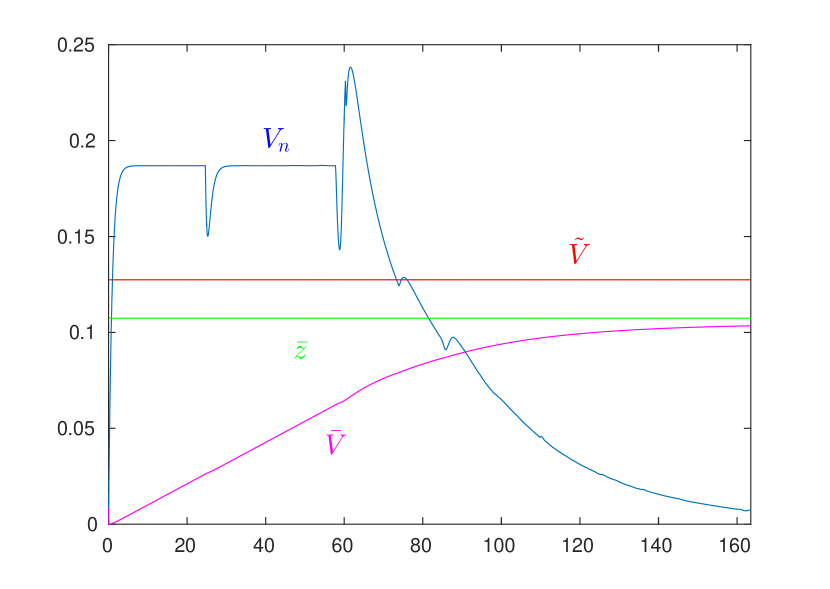
Figure 4: Demonstration of the maximum average relative velocity w.r.t. wind $\tilde{V}$, the average velocity $\bar{V}$ and the nominal mission velocity $V_{n}$ for a robot revolving around the charging station.

To estimate the time at which the neediest robot starts approaching the charging station $T_{start}$, we can approximate it as being the time at which $h_{e}=0$ for this robot, while supposing it is operating at the boundary of the operating range $\mathcal{R}$. This means

$$E(T_{start})-E_{min}(T_{start})-k_{c}\log\frac{R_{0}}{\delta}=0$$ (61)

we can take $E(t)=E_{max}-(k_{e}+k_{v}\tilde{V})(t-t_{0})$ where $t_{0}=0$ (considering the first cycle) and we can take $E_{min}(T_{start})=E_{M}$. Substituting in the last equation we get

$$T_{start}=\frac{E_{max}-E_{M}-k_{c}\log\frac{R_{0}}{\delta}}{k_{e}+k_{v}\tilde{V}}$$ (62)

substituting (27) in the last equation we get

$$\begin{split}T_{start}&=\frac{\varepsilon}{k_{e}+k_{v}\tilde{V}}\left(1-\frac{1}{1+\kappa(n-1)}\right)\\ &+\frac{n(E_{max}-E_{lb})-k_{c}(1+\kappa(n-1))\log\tfrac{R_{0}}{\delta}}{(1+\kappa(n-1))(k_{e}+k_{v}\tilde{V})}\end{split}$$ (63)

Supposing that the robot decreases its velocity from $V_{n}$ to $v_{f}$ in an amount of time equal to $T_{end}-T_{start}$, then

$$\begin{split}v_{f}=V_{n}e^{-a(T_{end}-T_{start})}\end{split}$$ (64)

and

$$a=-\frac{1}{T_{end}-T_{start}}\log\frac{v_{f}}{V_{n}}$$ (65)

Now in order to calculate the increase in $E_{min}$

$$\begin{split}\varepsilon&=k_{v}V_{n}\int_{0}^{T_{end}-T_{start}}(1-e^{-at})dt\\ &=k_{v}V_{n}\left[t+\frac{1}{a}e^{-at}\right]_{0}^{T_{end}-T_{start}}\\ &=k_{v}V_{n}\left[T_{end}-T_{start}+\frac{1}{a}\left(\frac{v_{f}}{V_{n}}-1\right)\right]\\ &=k_{v}V_{n}\underbrace{\left[1+\frac{1}{\log\frac{V_{n}}{v_{f}}}\left(\frac{v_{f}}{V_{n}}-1\right)\right]}_{\Gamma}(T_{end}-T_{start})\end{split}$$ (66)

the smaller the choice of $v_{f}$, the closer $\Gamma$ approaches one, and the more conservative the estimate of $\varepsilon$ will be. Substituting (60) and (63) in the above equation we get

$$\varepsilon=\frac{\Gamma k_{v}V_{n}\left(T_{end}-\tfrac{n(E_{max}-E_{lb})-k_{c}(1+\kappa(n-1)\log\tfrac{R_{0}}{\delta}}{(k_{e}+k_{v}\tilde{V})(1+\kappa(n-1)}\right)}{1+\tfrac{\Gamma k_{v}V_{n}}{k_{e}+k_{v}\tilde{V}}\left(1-\tfrac{1}{1+\kappa(n-1)}\right)}$$ (67)

References

• [1] D. Portugal and R. Rocha, “A survey on multi-robot patrolling algorithms,” in Doctoral conference on computing, electrical and industrial systems.   Springer, 2011, pp. 139–146.
• [2] J. Cortes, S. Martinez, T. Karatas, and F. Bullo, “Coverage control for mobile sensing networks,” IEEE Transactions on robotics and Automation, vol. 20, no. 2, pp. 243–255, 2004.
• [3] W. Burgard, M. Moors, C. Stachniss, and F. E. Schneider, “Coordinated multi-robot exploration,” IEEE Transactions on robotics, vol. 21, no. 3, pp. 376–386, 2005.
• [4] K. H. Petersen, R. Nagpal, and J. K. Werfel, “Termes: An autonomous robotic system for three-dimensional collective construction,” Robotics: science and systems VII, 2011.
• [5] Z. Sun and J. Reif, “On energy-minimizing paths on terrains for a mobile robot,” in 2003 IEEE International Conference on Robotics and Automation (Cat. No. 03CH37422), vol. 3.   IEEE, 2003, pp. 3782–3788.
• [6] S. Slijepcevic and M. Potkonjak, “Power efficient organization of wireless sensor networks,” in ICC 2001. IEEE International Conference on Communications. Conference Record (Cat. No. 01CH37240), vol. 2.   IEEE, 2001, pp. 472–476.
• [7] A. Kwok and S. Martinez, “Energy-balancing cooperative strategies for sensor deployment,” in 2007 46th IEEE Conference on Decision and Control.   IEEE, 2007, pp. 6136–6141.
• [8] Y. Ding, W. Luo, and K. Sycara, “Decentralized multiple mobile depots route planning for replenishing persistent surveillance robots,” in 2019 International Symposium on Multi-Robot and Multi-Agent Systems (MRS).   IEEE, 2019, pp. 23–29.
• [9] G. Notomista, S. F. Ruf, and M. Egerstedt, “Persistification of robotic tasks using control barrier functions,” IEEE Robotics and Automation Letters, vol. 3, no. 2, pp. 758–763, 2018.
• [10] H. Fouad and G. Beltrame, “Energy autonomy for resource-constrained multi robot missions,” in International Conference on Intelligent Robots and Systems (IROS), 2020.
• [11] A. D. Ames, S. Coogan, M. Egerstedt, G. Notomista, K. Sreenath, and P. Tabuada, “Control barrier functions: Theory and applications,” in 2019 18th European Control Conference (ECC).   IEEE, 2019, pp. 3420–3431.
• [12] A. D. Ames, X. Xu, J. W. Grizzle, and P. Tabuada, “Control barrier function based quadratic programs for safety critical systems,” IEEE Transactions on Automatic Control, vol. 62, no. 8, pp. 3861–3876, 2016.
• [13] X. Xu, P. Tabuada, J. W. Grizzle, and A. D. Ames, “Robustness of control barrier functions for safety critical control,” IFAC-PapersOnLine, vol. 48, no. 27, pp. 54–61, 2015.
• [14] W. Xiao and C. Belta, “Control barrier functions for systems with high relative degree,” in 2019 IEEE 58th Conference on Decision and Control (CDC).   IEEE, 2019, pp. 474–479.
• [15] A. Li, L. Wang, P. Pierpaoli, and M. Egerstedt, “Formally correct composition of coordinated behaviors using control barrier certificates,” in 2018 IEEE/RSJ International Conference on Intelligent Robots and Systems (IROS).   IEEE, 2018, pp. 3723–3729.
• [16] L. Wang, A. D. Ames, and M. Egerstedt, “Multi-objective compositions for collision-free connectivity maintenance in teams of mobile robots,” in 2016 IEEE 55th Conference on Decision and Control (CDC).   IEEE, 2016, pp. 2659–2664.
• [17] M. Egerstedt, J. N. Pauli, G. Notomista, and S. Hutchinson, “Robot ecology: Constraint-based control design for long duration autonomy,” Annual Reviews in Control, vol. 46, pp. 1–7, 2018.