Quantitative Security Risk Modeling and Analysis with RisQFLan

Abstract

Domain-specific quantitative modeling and analysis approaches are fundamental in scenarios in which qualitative approaches are inappropriate or unfeasible. In this paper, we present a tool-supported approach to quantitative graph-based security risk modeling and analysis based on attack-defense trees. Our approach is based on QFLan, a successful domain-specific approach to support quantitative modeling and analysis of highly configurable systems, whose domain-specific components have been decoupled to facilitate the instantiation of the QFLan approach in the domain of graph-based security risk modeling and analysis. Our approach incorporates distinctive features from three popular kinds of attack trees, namely enhanced attack trees, capabilities-based attack trees and attack countermeasure trees, into the domain-specific modeling language. The result is a new framework, called RisQFLan, to support quantitative security risk modeling and analysis based on attack-defense diagrams. By offering either exact or statistical verification of probabilistic attack scenarios, RisQFLan constitutes a significant novel contribution to the existing toolsets in that domain. We validate our approach by highlighting the additional features offered by RisQFLan in three illustrative case studies from seminal approaches to graph-based security risk modeling analysis based on attack trees.

I Introduction

Quantitative modeling and analysis approaches are essential to support software and system engineering in scenarios where qualitative approaches are inappropriate or unfeasible, e.g. due to complexity or uncertainty, or by the quantitative nature of the properties of interest. Automated approaches to support quantitative modeling and analysis have been developed extensively during the last decades, including generic as well as domain-specific approaches (cf., e.g., [1, 2, 3, 4, 5, 6, 7, 8, 9, 10]).

QFLan [8] is one example of a successful domain-specific approach to support quantitative modeling and analysis of highly configurable systems, such as software product lines. QFLan combines several well-studied rigorous notions and techniques in an Eclipse-based domain-specific tool framework. It consists of a domain-specific language (DSL) tailored for configurable systems, and an analysis engine based on statistical model checking (SMC) [11, 12]. In [8], we showed the robustness and scalability of QFLan by analyzing large instances of case studies that could not be analyzed before.

In this paper, we generalize the QFLan approach by decoupling domain-specific components and instantiating the QFLan approach in a new domain: risk modeling and analysis.

The result, called RisQFLan, is a new framework to support graph-based quantitative security risk modeling and analysis. It constitutes a significant novel contribution to existing toolsets in that domain. In particular, RisQFLan can be used to:

1. build rich models by combining distinctive features from existing formalisms for risk modeling and analysis;

2. enhance the analysis of existing tools for risk modeling.

Regarding 1), the DSL of RisQFLan has been designed to include the most significant features of existing formalisms based on attack trees, such that they can be combined in the same model. Subsets of the RisQFLan DSL, indeed, can thus be used to capture classes of existing modeling formalisms. In addition, RisQFLan allows one to focus on specific dynamic threat profiles, a feature that is being supported only recently by very few approaches ([13, 4, 5, 14, 15, 16]) and in a limited way (cf. the detailed discussion in Section VIII).

We validate feature 2) by showing in Section VII how three influential classes of risk models based on attack trees can be specified in RisQFLan, and how the RisQFLan analysis capabilities can be used to complement and enrich those provided by existing toolsets. This is an advantage offered with respect to the existing tools. In particular, RisQFLan includes an additional analysis engine based on exact probabilistic model checking that is not inherited from QFLan, which comes with a statistical model checking engine [17].

Synopsis

Section II introduces the domain of graph-based security risk modeling with attack-defense trees. Section III presents a first contribution of the paper: a generalization of the QFLan approach to domain-specific quantitative modeling and analysis. Sections IV-VI describe the main contributions of the paper to support security risk modeling and analysis: the RisQFLan DSL in Section IV, its formal semantics in Section V and the analysis capabilities of the RisQFLan tool in Section VI. Section VII validates the flexibility of RisQFLan by illustrating in detail how features from three influential classes of attack trees can be specified in RisQFLan and how the RisQFLan analysis capabilities can be successfully used to complement and enrich the analyses provided by existing tools. Section VIII discusses related work. Section IX draws conclusions and outlines future work.

II Graph-based Risk Modeling and Analysis

This section provides a brief introduction to the specific domain of risk modeling and analysis with graph-based security models. For this purpose, we use as running example the risk assessment of a “bank robbery” scenario, which will also be used in Section IV to illustrate RisQFLan.

Graph-based security models offer an intuitive and effective means to represent security scenarios in complex systems, by combining intuitive visual features with formal semantics, which can then be used for formal analysis. Attack trees and their variants [18, 19, 20] constitute a popular family of graph-based security models for which several approaches have been developed over the last years (cf., e.g., the surveys [21, 22, 23]), aiming at providing scalable and usable methods for specifying vulnerabilities and countermeasures, their interplay and their key attributes such as cost and effectiveness. Attack trees (and attack-defense trees) thus serve as a basis for quantitative risk assessment, which helps to determine, for instance, where defensive resources are best spent to protect a system.

In their simplest form, attack-defense diagrams are and/or-trees whose nodes represent either attack goals or defensive measures, and with sub-trees representing refinements of such goals and measures. Fig. 1 shows an attack-defense diagram modeling our running example. The tree’s root represents the main threat under analysis, i.e. robbing a bank (RobBank).

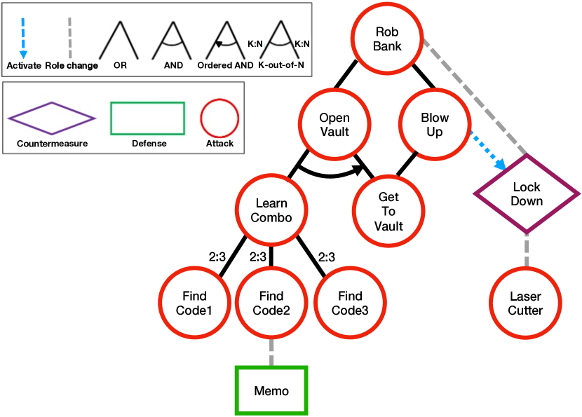
Figure 1: Attack-defense diagram

Attack nodes can be refined in several ways by identifying necessary sub-goals and combining them in different ways, e.g. with disjunction, (ordered) conjunction, etc. In our example, the attacker has two options to achieve its main goal: either open the vault (OpenVault) or blow it up (BlowUp). This is specified in the tree with corresponding nodes as children of node RobBank, combined in a disjunctive way. Another kind of refinement illustrated in our example is the following: in order to open the vault (OpenVault), the attacker needs to first learn its combo (LearnCombo) and then get to the vault (GetToVault). This is specified by combining LearnCombo and GetToVault through an ordered conjunction. A last example of refinement is used to model that for security reasons two out of three of the vault’s opening codes are required (FindCode1–FindCode3). Instead, blowing it up only requires to get to the vault.

Attack-defense diagrams can also include defensive mechanisms to deal with or to prevent attack threats. In the example scenario, there are two defensive mechanisms. First, a LockDown countermeasure, triggered by (successful or not) blow up attacks that, once active, mitigates bank robbery attacks. The rationale is that the vault is sealed to prevent robbery when an explosion is detected. The second defensive measure in our running example is a defense Memo, permanently active against attacks trying to find opening code 2 (FindCode2). The interplay between such a defensive countermeasure and the corresponding attack nodes is also typically depicted visually, as in our example. Defensive mechanisms, in turn, can also be affected (e.g. disabled or mitigated) by attacks. For instance, in our example an attack with a LaserCutter can break the LockDown.

Attack-defense diagrams, besides being a useful tool for modeling and informally reasoning on security risk scenarios, often also have a formal meaning that lies at the basis of formal reasoning, typically supported by effective software tools like SecurITree [24], ADTool [25], SPTool [26], and ATTop [16] to mention a few (cf. surveys [21, 23, 22] for further examples).

Standard analyses conducted on attack-defense diagrams typically regard the feasibility of attacks (e.g. can the attacker activate some actions that will result in the achievement of her/his main goal?), their likelihood (e.g. what is the probability that the main goal is achieved?) or their cost (e.g. what is the cheapest successful attack for the attacker?). Analysis techniques are often based on constraint solving, optimization and statistical techniques. Section VI will provide some of these analyses applied to our running example.

III Generalizing the QFLan Approach

This section describes how the QFLan architecture was made amenable for instantiation in domains beyond the one for which it was conceived (configurable systems like software product lines), and how its analysis capabilities were enriched.

The original QFLan architecture

We first summarize the original QFLan architecture as presented in [8], organized in two layers: the Graphical User Interface (GUI), devoted to modeling, and the CORE layer, devoted to analysis. Both layers are wrapped in an Eclipse-based tool embedding the third-party statistical analyzer MultiVeStA [27, 28]. QFLan is an open-source tool. The components of the GUI layer are:

• a QFLAN Editor with editing support that is typical of a modern Integrated Development Environment (IDE), developed in the XTEXT framework, and a MultiQuaTEx Editor for property specification in the MultiQuaTEx language [27];

• a set of Views, including a project explorer, a diagnosis console and a plot viewer for displaying analysis results.

The components of the CORE layer are:

• a Probabilistic Simulator, which is an interpreter of the formal semantics as probabilistic processes. This interacts with the external statistical analyzer MultiVeStA to obtain SMC capabilities;

• a Built-in Constraint Solver used by the simulator to check constraints during simulation.

The refactored QFLan architecture

The architecture illustrated in Fig. 2 decouples domain-specific components of the QFLan architecture from domain-generic ones. The domain-specific components that need to be provided to instantiate the architecture in a new domain are the following: the XTEXT grammar for DSL, the Interpreter, the Constraint Solver and the Model Visualizer (differentiated from other components by their blank background). The remaining components are either existing domain-generic components (solid border) or domain-specific components, automatically generated by XTEXT (dashed border).

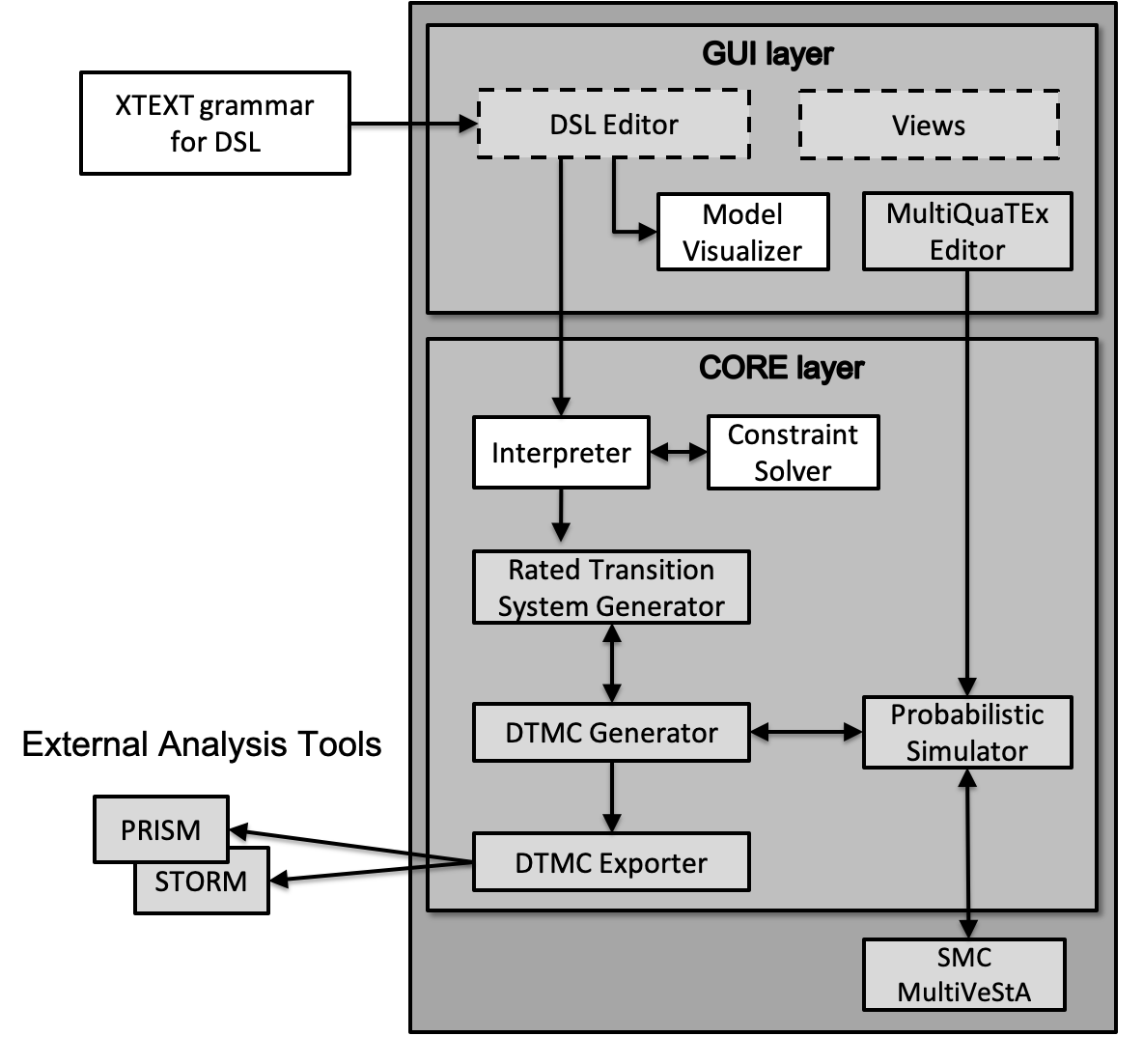
Figure 2: The refactored QFLan architecture

The GUI layer basically remains unchanged, except that Fig. 2 makes explicit that the DSL Editor is generated automatically from an XTEXT grammar for DSL. Moreover, it was extended with a Model Visualizer component to offer an automatic visual representation of the model at hand. This is obtained by providing an encoding of the models’ features of interest in the DOT language .

The main changes in the refactored QFLan architecture however concern the CORE layer, whose new components are:

• an Interpreter and a Constraint Solver, implementing the formal semantics of the DSL based on rated transition systems (transition systems with rate-decorated transitions);

• a Rated Transition System Generator relying on the Interpreter to generate rated transition systems on-the-fly;

• a DTMC Generator, which uses the Rated Transition System Generator to normalize rated transition systems into on-the-fly generated Discrete-Time Markov Chains (DTMC);

• a Probabilistic Simulator, which is now separated from the above components and which is able to simulate a DTMC without fully generating it using the on-the-fly DTMC Generator;

• a DTMC Exporter which generates an entire DTMC by using the DTMC Generator and exports it in the input format of the well-known probabilistic model checkers PRISM [29] (www.prismmodelchecker.org) and STORM [30] (www.stormchecker.org).

IV RisQFLan DSL

This section describes RisQFLan, a domain-specific instantiation of QFLan in the security risk domain described in Section II. A screenshot of RisQFLan is provided in Fig. 3, depicting the implemented components from the GUI layer in Fig. 2. We describe here the DSL of RisQFLan, while its formal semantics is given in Section V and its analysis capabilities are presented in Section VI. We illustrate the DSL of RisQFLan through the running example, whose attack-defense diagram is depicted in Fig. 1 (and in Fig. 3).

Figure 3: A screenshot of RisQFLan

In the DSL, nodes are declared in specific blocks, cf. Code 1. Note that countermeasure nodes require to indicate the attack node(s) that may trigger them.

⬇

begin attack nodes

RobBank OpenVault BlowUp

LearnCombo GetToVault

FindCode1 FindCode2

FindCode3 LaserCutter

end attack nodes

begin defense nodes

Memo

end defense nodes

begin countermeasure nodes

LockDown = {BlowUp}

end countermeasure nodes

Code 1: Nodes

Our attack-defense diagrams relate nodes by two types of relations: (i) refinements shape offensive (defensive, resp.) nodes into a set of offensive (defensive, resp.) sub-nodes; (ii) role-changes state how to oppose offensive (defensive, resp.) nodes by defensive (offensive, resp.) nodes. Each node has at most one refinement and at most one role-change. Typical for our approach is that nodes may have multiple parents, which is convenient to specify an attack (defense) node that affects multiple defenses (attacks) or an attack (defense) node that refines many attacks (countermeasures).

We offer OR, AND, OAND (ordered AND), and k-out- of-n refinements for attack and countermeasure nodes. Defense nodes model static, atomic defenses that cannot be refined. Countermeasures are also atomic, but they can be refined with defense nodes to permit reactive defense nodes that become effective only upon (attack detection and) activation of the refined countermeasure. AND and OR refinements originate from the seminal works on attack trees [18]. OAND refinements stem from enhanced and improved attack trees [31, 32] and are used to model ordered attacks: sub-nodes can be activated in any order but only the correct order activates the parent node. The k-out-of-n refinements are inspired by attack countermeascure trees [33].

Lines 2-5 of Code 2 show how to declare attack diagrams in RisQFLan. The square brackets of OAND indicate that order matters: OpenVault requires LearnCombo and GetToVault in that order. K2 expresses that at least two of the three sub-attacks of LearnCombo are required. Inspired by other formalisms supporting both attack and defense mechanisms, like attack-defense trees [20], a role-changing relation describes the attack a countermeasure or defense works against (e.g. LockDown defends against RobBank) or vice versa (e.g. LaserCutter neutralizes LockDown). Lines 6-8 of Code 2 show that attack, defense and countermeasure nodes can additionally have a role-changing relation with a child of the opposite role, an opponent node affecting its activation.

⬇

1begin attack diagram

2 RobBank -> {OpenVault, BlowUp}

3 OpenVault -OAND-> [LearnCombo, GetToVault]

4 BlowUp -> {GetToVault}

5 LearnCombo -K2-> {FindCode1, FindCode2, FindCode3}

6 RobBank -> {LockDown}

7 LockDown -> {LaserCutter}

8 FindCode2 -> {Memo}

9end attack diagram

Code 2: Attack-defense diagram

As in other approaches [21], attack nodes may be decorated with attributes, like cost or detection rates, for quantitative analyses [34, 5, 15]. The cost of (attempting) an attack, like the attribute Cost in Code 3, may be used to impose constraints. The default value is $0$, e.g. $\texttt{Cost(GetToVault)}\!=\!0$. The cumulative value for the entire scenario, often the cost associated to a (sub-system rooted in a) node, is the sum of the costs of its active descendants [18]. However, the total cost of an attack should not reflect only the cost of successful sub-attacks, as this would be a best-case scenario. Therefore, in RisQFLan we consider both successful and failed attack attempts to compute the value of an attribute of an attack node. Furthermore, we allow attributes also for defensive nodes.

⬇

begin attributes

Cost = {LaserCutter = 10, BlowUp = 90,

FindCode1 = 5, FindCode2 = 5, FindCode3 = 5}

end attributes

Code 3: Attributes

In [24, 35], a noticeability attribute is a behavioral metric used to indicate the likeliness of an attack attempt to be noticed. Following attack countermeasure trees [33], we make this notion a first-class citizen of RisQFLan, called attack detection rate, which influences activation of countermeasures. More precisely, such a rate determines the

⬇

begin attack detection rates

BlowUp = 1.0

end attack detection rates

Code 4: Attack detection rates

probability for an attack attempt, whether successful or not, to be detected, and it triggers the activation of the affected countermeasures, in the sense that higher detection rates lead to more likely activation of countermeasures. The default value is $0$, i.e. an attack is undetectable. Code 4 shows that an attempt to blow up a vault is always noticed.

In [20, 25], an attack node is disabled if it is affected by a defense. However, a common conception in security is that nothing is 100% secure. Therefore, we include the notion of defense effectiveness from [33] to specify the probability for a defense node to be effective against a combination of attack nodes and attack behavior. The rationale is that different attackers might be affected differently, even when attempting the same attack (e.g. a security guard is efficient against a thief, but not against a military attack). The default value is $0$, i.e. the defense has no effect. Code 5 states that Memo scales the probability of succeeding in FindCode2 attacks by $1-0.5$, whereas LockDown scales that of RobBank by $1-0.3$.

⬇

begin defense effectiveness

Memo(ALL, FindCode2) = 0.5, LockDown(ALL, RobBank) = 0.3

end defense effectiveness

Code 5: Defense effectiveness (ALL denotes any attacker)

IV-A Attack Behavior

An important feature of our models is that defensive behavior is reactive, while attackers are proactive. RisQFLan allows to fine tune security scenarios by defining explicit attack behavior, implicitly constrained by an attack-defense diagram. The combination of attack-defense diagrams and explicit (probabilistic) attack behavior was motivated by work on configurable systems [8, 36]. Explicit attack behavior enables the analyses of specific attacker types, like script kiddies, insiders, and hackers, which has the advantage of being able to evaluate system vulnerabilities for those attacker types that make more sense for the security scenario at hand. Moreover, it enables novel types of analysis to complement the classical best- and worst-case evaluations of attack graphs (like the bottom-up evaluation in ADTool [25]).

Attack behavior is modeled as rated transition systems, whose transitions are labeled with the action being executed and a rate (used to compute the probability of executing the action), and possibly with effects (updates of variables) and guards (conditions on the action’s executability), in this order (e.g. Lines LABEL:ls:order1-LABEL:ls:order2 in Code 7). Fig. 4 (and its corresponding Code 7) sketches an attacker, named Thief, that starts by choosing to attempt an open vault (tryOpenVault) or blow up (tryBlowUp) attack. Independently of this choice, s/he can try get-to-vault attacks (tryGetToVault), required by both strategies. OpenVault requires to try to learn the combo, which in turn requires to try to find at least two codes.

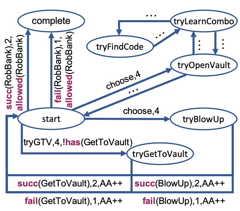
Figure 4: Attack behavior

⬇

begin actions

choose tryGTV try

end actions

Code 6: Actions

Attacker actions can be user-defined for scenario-specific behavior not directly related to node activation, such as those in Code 6 (where try is part of the attacks tryOpenVault, tryLearnCombo and tryFindCode that are not further detailed in Fig. 4 and Code 7). RisQFLan also provides a set of predefined attacker actions, like succ and fail for a successful or failed attack attempt, resp., modeled by a probabilistic choice between succ and fail actions, whose associated rates determine the success likelihood together with (the effectiveness of) the involved defenses. In Section VII, we will see how attackers can apply backtracking strategies via the predefined action remove.

Attack behavior is executed by considering, at each step, the outgoing transitions from the current state admitted by the attack diagram and by further constraints discussed below. Normalizing the sum of the rates of these transitions to 1 leads to a DTMC, while probabilistic simulations are obtained by selecting one transition probabilistically using the transition rates (e.g., from start to complete with probability $\frac{1}{1+2}$).

Transitions can contain guards, like allowed, used to attempt RobBank in start only if all required sub-attacks succeeded (cf. Lines LABEL:ls:start-LABEL:ls:start2 in Code 7), or !has, used to forbid the transition to tryGetToVault if one already succeeded to GetToVault (cf. Line LABEL:ls:vault in Code 7).

⬇

1begin attacker behavior@\label{ls:attbhv}begin attack attacker = Thief states = start, tryOpenVault, tryLearnCombo, tryFindCombo, tryGetToVault, tryBlowUp, complete\label{ls:attstates}transitions = start -(succ(RobBank), 2, allowed(RobBank)) -> complete, //If I open or blow up the vault, then I can rob the bank\label{ls:start}start -(fail(RobBank), 1, allowed(RobBank)) -> complete,\label{ls:start2}start -(tryGTV, 4, !has(GetToVault)) -> tryGetToVault, //Whatever strategy was used, I must get to the vault\label{ls:vault}tryGetToVault -(succ(GetToVault), 2, AttackAttempts=AttackAttempts+1) -> start, tryGetToVault -(fail(GetToVault), 1, AttackAttempts=AttackAttempts+1) -> start,\label{ls:vault2}start -(choose, 4) -> tryOpenVault, //This is the strategy where I open the vault tryOpenVault -(succ(OpenVault), 2, AttackAttempts=AttackAttempts+1, has(LearnCombo) and has(GetToVault)) -> start,\label{ls:order1}tryOpenVault -(fail(OpenVault), 2, AttackAttempts=AttackAttempts+1, has(LearnCombo) and has(GetToVault)) -> start,\label{ls:order2}tryOpenVault -(try, 2, has(LearnCombo) and !has(GetToVault)) -> start, //I know the combo but did not get to the vault tryOpenVault -(try, 5, !has(LearnCombo)) -> tryLearnCombo, ... //Similar for tryLearnCombo and then tryFindCode start -(choose, 4) -> tryBlowUp, //This is the strategy where I blow up the vault tryBlowUp -(succ(BlowUp), 2, AttackAttempts=AttackAttempts+1) -> start, tryBlowUp -(fail(BlowUp), 1, AttackAttempts=AttackAttempts+1) -> start end attack end attacker behavior\label{ls:attbhv2}

Code 7: Attack behavior

RisQFLan also supports action constraints, acting as guards on any transition executing a given action (while transition guards constrain single transitions). They are given as do$(\textit{act\/})\rightarrow b$, where act is an action and $b$ is a Boolean expression over attributes. As defined in Code 8, any transition with action choose is disabled as soon as one succeeds to open or blow up the vault.

⬇

begin action constraints

do(choose) -> !(has(OpenVault) or has(BlowUp))

end action constraints

Code 8: Action constraints

Transitions can also be labeled with side-effects: real-valued variables updated upon a transition’s execution. Variables model context information, thus allowing for rich descriptions of system states, of attackers and of defenses, greatly facilitating the expression of constraints and the analysis phase. Code 9 defines variable AttackAttempts (AA in Fig. 4), which stores the number of attack attempts, updated each time a succ or fail action occurs as attempt to rob the bank.

⬇

begin variables

AttackAttempts = 0

end variables

Code 9: Variables

⬇

begin quantitative constraints

{value(Cost) <= 100}

end quantitative constraints

Code 10: Quantitative constraints

In addition to constraints imposed by attack diagrams, transition guards and action constraints, attack behavior may be constrained by quantitative constraints in the form of Boolean expressions involving (arithmetic expressions or inequalities over) reals, attributes and variables. In Code 10, we constrain to 100 the maximum accumulated cost of an attack, of particular interest since attack behavior may model failed attacks.

Attack behavior is completed with an initial setup specifying the attacker and any initially accomplished attack(s). The latter

⬇

begin init

Thief = {FindCode1}

end init

Code 11: Initial setup

enrich expressiveness, since one can assign an initial advantage to attackers: an attack-defense diagram models all possible attacks, but some attackers (e.g., insiders) may already have access to critical components. This is convenient as a diagram’s sub-trees may be ignored without their explicit removal. Due to Code 11, the attacker Thief already has one code.

Note that RisQFLan provides a programming-like environment that may be attractive to software developers, but it integrates at the same time a graphical component shown in Fig. 3, which may make it more attractive for security experts. The DSL moreover has a formal semantics, defined next.

V RisQFLan Operational Semantics

V-A RisQFLan Models and Configurations

In this section, we provide a formal definition of the ingredients composing RisQFLan models. In order to improve readability, we provide references to the corresponding code blocks from Section IV when relevant, which show ho the components of the model are actually specified in our DSL.

A RisQFLan model $\mathcal{S}$ is defined as a septuple $\mathcal{S}=\langle\mathcal{N},\mathcal{D},\mathcal{V},\mathcal{A},\mathcal{B},\mathcal{C},\mathcal{P}\rangle$, where

• $\mathcal{N}=\mathcal{N}_{a}\uplus\mathcal{N}_{d}\uplus\mathcal{N}_{c}$ is a set of nodes divided into attack nodes $\mathcal{N}_{a}$, defense nodes $\mathcal{N}_{d}$ and countermeasure nodes $\mathcal{N}_{c}$ (Code 1);

• $\mathcal{D}$ is a set of attacker actions. The set $\mathcal{D}$ contains all actions succ($n_{a}$), fail($n_{a}$), and remove($n_{a}$), where $n_{a}\in\mathcal{N}_{a}$, and additionally user-defined actions (Code 6);

• $\mathcal{V}$ is a set of variables (Code 9);

• $\mathcal{A}$ is a set of attackers names (Code 7);

• $\mathcal{B}$ is a set of attacker behaviors (Code 7);

• $\mathcal{C}$ is a set of constraints on the (presence/absence of) nodes, their attributes, and on (user-defined) variables. Such constraints are formed by the hierarchical constraints (built with -OR->, -AND->, -OAND->, and -Kn->, Code 2), action constraints (of the form do$(\textit{act\/})\rightarrow b$, where $\textit{act\/}\in\mathcal{D}$ and $b$ is a Boolean expression over attributes, Code 8) and quantitative constraints (Boolean expressions enriched with special attributes like allowed($n_{a}$) and has($n_{a}$), with $n_{a}\in\mathcal{N}_{a}$, Code 10);

• $\mathcal{P}:\mathcal{N}\rightarrow\mathbb{R}$ is a set of node properties, distinguishing attributes decorating nodes (Code 3), attack detection rates decorating attack nodes (functions $\mathcal{N}_{a}\rightarrow[0,1]$, Code 4) and defense effectiveness decorating defense nodes (functions $(\mathcal{N}_{d}\cup\mathcal{N}_{c})\times\mathcal{N}_{a}\times\mathcal{A}\rightarrow[0,1]$, Code 5).

We introduce the notion of configuration for a RisQFLan model and equip it with an operational semantics based on rated transition systems. A configuration of a RisQFLan model $\mathcal{S}$ is a tuple $\langle C,s\rangle$, where $s$ is a state of attack behavior of $\mathcal{S}$ and $C$ is a set of constraints consisting of:

• all constraints of the model $\mathcal{S}$;

• a predicate $\textit{has}(n)$ for each currently active node $n\in\mathcal{N}$;

• constraints of form $t(n_{a})<t(n_{a}^{\prime})$, for $n_{a},n_{a}^{\prime}\in\mathcal{N}_{a}$, denoting that $n_{a}$ was activated before $n^{\prime}_{a}$, necessary to support OAND refinements;

• an assignment of form $\textit{att}(n)=x$ for each attribute att and node $n\in\mathcal{N}$ to denote the value of the attribute for the node $n$, with $x\in\mathbb{R}$;

• assignments of form $\textit{value}_{a}(\textit{att})=x$ and $\textit{value}_{\textit{def}}(\textit{att})=x$ for each attribute att to denote its cumulative attacker and defender value, with $x\in\mathbb{R}$;

• an assignment of form $v=x$ for each variable $v\in\mathcal{V}$, with $x\in\mathbb{R}$;

• an assignment of form $\textit{dr}(n_{a})=x$ for each attack node $n_{a}$ to denote detection rate of $n_{a}$, with $x\in\mathbb{R}$;

• a set $\textit{detect}(n_{c})\subseteq\mathcal{N}_{a}$ for each countermeasure node $n_{c}$ to denote the attack nodes that can be detected by $n_{c}$.

Let $\mathcal{M}$ denote the set of all configurations for a RisQFLan model $\mathcal{S}$. We restrict to configurations $\langle C,s\rangle$ such that $C$ is consistent, i.e. all constraints are satisfied, denoted by $\textit{con}(C)$. As we will see in Proposition 1, this property is preserved by the operational semantics: no inconsistent configuration can be reached from a consistent one. We will use $\oplus$ to denote union of constraint sets, $\ominus$ for subtraction and $\vdash$ for entailment.

V-B RisQFLan Dynamics

The dynamics of RisQFLan configurations is given as rated transition systems that specify how a configuration $\langle C,s\rangle$ can evolve into a configuration $\langle C^{\prime},s^{\prime}\rangle$ with a certain rate $r$. Such evolution occurs as the consequence of the attacker trying to perform an action and the defender eventually reacting to mitigate it. We denote such an evolution with a transition of the form $\langle C,s\rangle\xrightarrow[]{r}\langle C^{\prime},s^{\prime}\rangle$. In general, the dynamics is defined by a multi-relation $\rightarrow\subseteq\mathbb{N}^{\mathcal{M}\times\mathbb{R^{+}}\times\mathcal{M}}$ induced by the rules of Fig. 5. We use a multi-relation since we have to account for multiple copies of the same transition with the same rate, as the probabilistic interpretation requires to ‘sum’ such rates. Indeed, as we shall see, the dynamics of a configuration is ultimately defined as a discrete-time Markov chain, upon which the analysis of RisQFLan is based.

$$\inference[\scriptsize\textsc{[Act]}]{s\xrightarrow{\textit{act\/},r,u,g}s^{\prime}\qquad\textit{exe\/}(C,act,g)\qquad C^{\prime}=u(C,\textit{act\/})\qquad\textit{con}(C^{\prime})}{\langle C,s\rangle\xrightarrow[]{r}\langle C^{\prime},s^{\prime}\rangle}$$

$$\inference[\scriptsize\textsc{[Add]}]{s\xrightarrow{\textit{add\/}(n_{a}),r,u,g}s^{\prime}\qquad\textit{exe\/}(C,\textit{add\/}(n_{a}),g)\qquad\qquad\\ C^{\prime}=u(C,\textit{add\/}(n_{a}))\oplus\textit{has\/}(n_{a})\oplus\bigoplus\limits_{n_{c}\,\in\,c(n_{a},C)}\textit{has\/}(n_{c})\oplus\bigoplus\limits_{\{\,n\,\in\,\mathcal{N}_{a}\,\mid\,\textit{has\/}(n)\,\in\,C\,\}}t(n)<t(n_{a})\ominus\left(\bigoplus\limits_{\{\,n\,\mid\,n\leavevmode\nobreak\ \texttt{-RC->}\leavevmode\nobreak\ n_{a}\,\}}\textit{has\/}(n)\right)\qquad\textit{con}(C^{\prime})}{\langle C,s\rangle\xrightarrow[]{r\cdot\textit{de}(C^{\prime},n_{a},s)\cdot\textit{dr}(n_{a})}\langle C^{\prime},s^{\prime}\rangle}$$

$$\inference[\scriptsize\textsc{[AddNoC]}]{s\xrightarrow{\textit{add\/}(n_{a}),r,u,g}s^{\prime}\qquad\textit{exe\/}(C,\textit{add\/}(n_{a}),g)\qquad\qquad\\ C^{\prime}=u(C,\textit{add\/}(n_{a}))\oplus\textit{has\/}(n_{a})\oplus\bigoplus\limits_{\{\,n\,\in\,\mathcal{N}_{a}\,\mid\,\textit{has\/}(n)\,\in\,C\,\}}t(n)<t(n_{a})\ominus\left(\bigoplus\limits_{\{\,n\,\mid\,n\leavevmode\nobreak\ \texttt{-RC->}\leavevmode\nobreak\ n_{a}\,\}}\textit{has\/}(n)\right)\qquad\textit{con}(C^{\prime})}{\langle C,s\rangle\xrightarrow[]{r\cdot\textit{de}(C^{\prime},n_{a},s)\cdot(1-\textit{dr}(n_{a}))}\langle C^{\prime},s^{\prime}\rangle}$$

$$\inference[\scriptsize\textsc{[Fail]}]{s\xrightarrow{\textit{fail\/}(n_{a}),r,u,g}s^{\prime}\qquad\textit{exe\/}(C,\textit{fail\/}(n_{a}),g)\qquad C^{\prime}=u(C,\textit{fail\/}(n_{a}))\oplus\bigoplus\limits_{n_{c}\in c(n_{a},C)}\textit{has\/}(n_{c})\qquad\textit{con}(C^{\prime})}{\langle C,s\rangle\xrightarrow[]{r\cdot\textit{de}(C^{\prime},n_{a},s)\cdot\textit{dr}(n_{a})}\langle C^{\prime},s^{\prime}\rangle}$$

$$\inference[\scriptsize\textsc{[FailNoC]}]{s\xrightarrow{\textit{fail\/}(n_{a}),r,u,g}s^{\prime}\qquad\textit{exe\/}(C,\textit{fail\/}(n_{a}),g)\qquad C^{\prime}=u(C,\textit{fail\/}(n_{a}))\qquad\textit{con}(C^{\prime})}{\langle C,s\rangle\xrightarrow[]{r\cdot\textit{de}(C^{\prime},n_{a},s)\cdot(1-\textit{dr}(n_{a}))}\langle C^{\prime},s^{\prime}\rangle}$$

$$\inference[\scriptsize\textsc{[Rem]}]{s\xrightarrow{\textit{remove\/}(n_{a}),r,u,g}s^{\prime}\qquad\textit{exe\/}(C,\textit{remove\/}(n_{a}),g)\qquad\qquad\\ C^{\prime}=u(C,\textit{remove\/}(n_{a}))\ominus\left(\textit{has\/}(n_{a})\oplus\bigoplus\limits_{\{\,n\,\mid\,\textit{has\/}(n)\in C\,\}}t(n)<t(n_{a})\right)\qquad\textit{con}(C^{\prime})}{\langle C,s\rangle\xrightarrow[]{r}\langle C^{\prime},s^{\prime}\rangle}$$

Figure 5: Operational semantics

The rules share some premises and effects. First, all rules need an attack behavior transition of the form $s\xrightarrow{\alpha,r,u,g}s^{\prime}$, with current state of the attacker $s$, action $\alpha$, rate $r$ and memory update $u$, such that the executability conditions of the transition guard $g$ hold. This is imposed by exe($C,\alpha,g$), defined as:

$$\footnotesize\textit{exe\/}(C,\alpha,g)\!=\!\begin{cases}\textit{false}\!\!&\!\!\text{if $C\nvdash g$}\\ \textit{false}\!\!&\!\!\text{if $C=C^{\prime}\oplus(\textit{do\/}(\alpha)\rightarrow C^{\prime\prime})$ and $C^{\prime}\nvdash C^{\prime\prime}$}\\ \textit{false}\!\!&\!\!\text{if $\alpha\!=\!\textit{add\/}(n_{a})$ and $\textit{has\/}(n_{a})\!\in\!C$, with $n_{a}\!\in\!\mathcal{N}_{a}$}\\ \textit{false}\!\!&\!\!\text{if $\alpha\!=\!\textit{fail\/}(n_{a})$ and $\textit{has\/}(n_{a})\!\in\!C$, with $n_{a}\!\in\!\mathcal{N}_{a}$}\\ \textit{false}\!\!&\!\!\text{if $\alpha\!=\!\textit{remove\/}(n_{a}\mkern-1.0mu)$ and $\textit{has\/}(n_{a}\mkern-1.0mu)\!\not\in\!C$,\,with $n_{a}\!\in\!\mathcal{N}_{a}$}\\ \textit{true}\!\!&\!\!\text{otherwise\/}\end{cases}$$

Second, all rules require the resulting store to be consistent. Further conditions vary from rule to rule, as we will explain. By applying a rule on a configuration $\langle C,s\rangle$ due to a local transition $s\xrightarrow{\alpha,r,u,g}s^{\prime}$, we obtain a configuration $\langle C^{\prime},s^{\prime}\rangle$, where $C^{\prime}$ is obtained by applying the effects $u$ on the variables in $C$ (denoted $u(C,\alpha)$) and by possibly (de)activating nodes. In addition, $u(C,\alpha)$ updates cumulative attack and defense attribute values, as explained in Section IV. The semantics of $u(C,\alpha)$ is as expected, and not presented for conciseness.

We now describe each rule in detail.

Rule Act executes user-defined actions: node activations are not altered by this rule so its effects are limited to variables.

Rule Add is triggered by actions $\textit{add}(n_{a})$: with probability $\textit{dr}(n_{a})$, it may activate the set $c(n_{a},C)$ of countermeasure nodes able to detect $n_{a}$ that are not already active or inhibited by an active attack node $n^{\prime}_{a}$. The set $c(n_{a},C)$ is definedas follows, where -RC-> denotes a role-changing relation:

$$\{\,n_{c}\mid n_{a}\in\textit{detect}(n_{c})\wedge\textit{has}(n_{c})\not\in C\wedge\neg\exists n^{\prime}_{a}.\\ (\textit{has}(n^{\prime}_{a})\in C\wedge(n_{c}\leavevmode\nobreak\ \texttt{-RC->}\leavevmode\nobreak\ n^{\prime}_{a})\in C)\,\}$$

Upon the execution of the rule, the constraint store is updated with the new attack node $n_{a}$, which is recorded to be the last active attack node of the store ($t(n)<t(n_{a})$). Furthermore, the constraint store is also updated with each countermeasure node in $c(n_{a},C)$. Another effect is that all defenses that have $n_{a}$ as opponent are deactivated. The rate of the obtained transition is not necessarily the original rate $r$ of the attack behavior transition. In fact, $r$ might be scaled by the defense effectiveness of the active defenses against $n_{a}$ in the newly obtained store, denoted by $\textit{de}(C^{\prime},n_{a},s)\in[0,1]$. We distinguish three cases: (i) if $n_{a}$ has no role-changing relation, it is $1$; (ii) if $n_{a}$ has a defense opponent $n_{d}$, it is the effectiveness of $n_{d}$ for $n_{a}$ and the current attacker; (iii) if $n_{a}$ has a countermeasure opponent $n_{c}$, it is the product of the effectiveness of $n_{c}$ and that of any defense node that refines it, for $n_{a}$ and the attacker $\mathcal{A}$. Finally, we have to multiply the rate by the probability of activating the countermeasures, $\textit{dr}(n_{a})$. Rule AddNoC is similar, but it covers the case in which the countermeasures $c(n_{a},C)$ do not get activated.

Rules Fail and FailNoC are similar to Add and AddNoC, but the attack node is not activated because they regard the fail action which model failed attack attempts. Finally, rule Rem models the deactivation of an attack node.

It is easy to see that the semantic rules ensure consistency is preserved along sequences of configurations, since consistency is a premise in every rule, and hence in every transition.

Proposition 1

Let $\mathcal{S}$ be a RisQFLan model and $\langle C,s\rangle$ be a configuration such that $C$ is consistent. Then for any configuration $\langle C^{\prime},s^{\prime}\rangle$ such that $\langle C,s\rangle\rightarrow^{*}\langle C^{\prime},s^{\prime}\rangle$ it holds that $C^{\prime}$ is consistent.

The probabilistic interpretation of rated transition systems yields DMTCs. A DTMC is a tuple $\langle\Gamma,\Pi\rangle$ where $\Gamma$ is a set of states and $\Pi:\Gamma\rightarrow[0,1]$ is a probability transition function, i.e. such that for all $s\in\Gamma$, $\sum_{s^{\prime}\in\Gamma}\,\Pi(s,s^{\prime})=1$. The DTMC semantics of a rated transition system is obtained by normalising the rates into $[0..1]$ such that in each state/configuration, the sum of the rates of its outgoing transitions equals one. So, for a rated transition system $\rightarrow$ on a set of configurations $\mathcal{M}$ we obtain the DTMC $\langle\mathcal{M},\Pi\rangle$ where, for each pair of states $s,s^{\prime}\in\mathcal{M}$, the probability transition function $\Pi$ is defined by

$$\Pi(s,s^{\prime})=\begin{cases}\frac{\sum_{(s,r,s^{\prime})\in\rightarrow}\,r}{\mathbf{out}(s)}&\text{ if }\mathbf{out}(s)>0\\ 1&\text{ if }\mathbf{out}(s)=0\text{ and }s=s^{\prime}\\ 0&\text{ otherwise }\end{cases}$$

where $\mathbf{out}$ denotes the outdegree of a configuration. Note that self-loops with probability $1$ are added to configurations without outgoing transitions. The DTMC semantics of RisQFLan models is used in our analyses, described in the next section.

VI RisQFLan Supported Quantitative Analyses

RisQFLan supports the quantitative analysis of probabilistic attack scenarios by means of statistical model checking (SMC) [11, 12] as well as probabilistic model checking (PMC) [37], thus providing additional analysis capabilities to what other risk analysis tools typically offer.

SMC is concerned with running a sufficient number of (probabilistic) simulations of a system model to obtain statistical evidence (with a predefined level of statistical confidence) for the quantitative properties to be checked. Compared to obtaining exact results (with 100% confidence) with exact analysis techniques like (probabilistic) model checking, SMC offers unique advantages over exhaustive (probabilistic) model checking. Most importantly, SMC scales better. First, there is no need to generate entire state spaces, thus avoiding the combinatorial state-space explosion problem typical of model checking [17]. Second, the set of simulations to be carried out can be trivially distributed and run in parallel, thus scaling better with hardware resources. MultiVeStA, indeed, can be run on multi-core machines, clusters or distributed computers with a nearly linear speedup. Another advantage concerns its uptake in industry. Compared to model checking, SMC is simple to implement, understand and use, and it requires no specific modeling effort other than a system model that can be simulated and checked against quantitative properties. In fact, SMC is more and more being applied in industry [38, 39, 40, 41, 42, 43, 44, 45, 46, 47, 48, 49, 50].

In RisQFLan, the SMC analysis is obtained thanks to the internal DTMC simulator with MultiVeStA [27, 28], a framework for enriching simulators with SMC capabilities, while the PMC analysis is obtained thanks to RisQFLan’s DTMC exporting capabilities in a format supported by PRISM [29] and STORM [30]. SMC is necessary because the RisQFLan DSL has high expressivity, allowing for potentially unbounded variables and high variability in the models, thus often giving rise to large or infinite state spaces. PMC can instead be used for models with finite state spaces for exact analyses.

Next we showcase two SMC analysis capabilities of RisQFLan on our running example. PMC cannot be used in this case as the model has an infinite state space. We will showcase PMC analyses using PRISM in Section VII.

VI-A Analysis while Varying Simulation Steps

We start by studying the probabilities of activating attacks and countermeasures while varying the simulation step. This is expressed in Code 12: The pattern from-to-by specifies that we are interested in the first $100$ steps. We list $8$ properties of interest ($1$ per attack node, considering FindCode1 active, plus countermeasure LockDown). Each property can be an arithmetic expression of nodes (evaluating to $1$ or $0$ if the node is active or not, respectively), variables or attributes. The properties are considered in all $100$ steps, totaling $800$ properties.

⬇

begin analysis@\label{anafrom1}query = eval from 1 to 100 by 1 : RobBank, OpenVault, BlowUp, LearnCombo, GetToVault, FindCode2, FindCode3, LockDown default delta = 0.1 alpha = 0.1 parallelism = 1 end analysis\label{anafrom2}

Code 12: Analysis of the scenario

Each such actual property $p_{i}$ denotes a random variable $X_{i}$ which gets a real value assigned in each simulation. MultiVeStA estimates the expected value $E[X_{i}]$ of each of the $800$ properties (reusing the same simulations) as the mean $\overline{x}_{i}$ of $n$ independent simulations, with $n$ large enough to guarantee an $(\alpha,\delta)$ confidence interval (CI): $E[x_{i}]$ belongs to $[\overline{x}_{i}-\nicefrac{{\delta\!}}{{2}},\overline{x}_{i}+\nicefrac{{\delta\!}}{{2}}]$ with statistical confidence $(1-\alpha)\cdot 100\%$. The CI is given by alpha and default delta (but a property-specific $\delta$ could be used instead). Finally, parallelism states how many local processes should be launched to distribute the simulations. Overall the analysis required $400$ simulations, performed in $16$ seconds on a standard laptop machine.

Fig. 6 shows the results. Recall (Fig. 1, Code 2) that RobBank requires OpenVault or BlowUp. The probability to activate RobBank starts growing after step 4, stabilizing at $0.17$, while those of OpenVault and BlowUp reach $0.15$ and $0.11$, resp. We know from Code 8 that they cannot both be activated, so one should be able to activate RobBank with probability almost $0.26$. Instead, the actual probability is scaled down by $\frac{2}{3}$ due to the probabilistic choice from start to complete in Fig. 4: RobBank can either succeed or fail.

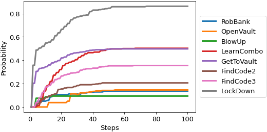
Figure 6: Analysis result of the properties in Code 12

Note that LockDown has a high probability to be activated, reaching about $0.85$ after $60$ steps. This is coherent with Code 5, stating that any BlowUp attempt is detected. One might expect the probability to activate BlowUp to be higher than that of LockDown, as the former triggers the latter. However, this is not true. This is explained by the fact that both succeeded and failed BlowUp attempts are detected (cf. success succ(BlowUp) and failure fail(BlowUp) actions in Fig. 4). Interestingly, if we added LaserCutter to the initial configuration, then the probability of activating LockDown would remain $0$, as it is inhibited by LaserCutter.

VI-B Analysis at the Verification of a Condition

We can also compute properties evaluated as soon as a given condition verifies. Here we compute the probability for each attack node to be the first attempted and succeeded, as well as the average number of steps needed to perform the first attempt. Code 13 expresses these $9$ properties ($1$ probability per attack node plus the average number of steps). Note that the from-to-by pattern is replaced by when to specify that the properties should be evaluated in the first state satisfying AttackAttempts == 1. Moreover, the list of properties of interest now includes steps, for which we give a specific delta, evaluated as the average number of steps computed to reach the first state satisfying the required condition.

⬇

begin analysis

query = eval when {AttackAttempts == 1} :

{RobBank, OpenVault, BlowUp, LearnCombo, GetToVault,

FindCode2, FindCode3, LockDown, steps[delta = 0.5]}

default delta = 0.1 alpha = 0.1 parallelism = 1

end analysis

Code 13: Analysis of the scenario

Rob	Open	Blow	Learn	GetTo	Find	Find	Lock	steps
Bank	Vault	Up	Combo	Vault	Code2	Code3	Down
0	0	0	0	0.27	0	0.01	0.32	2.51

Table I: Analysis result of the properties in Code 13

Overall, the analysis required $400$ simulations, performed in a few seconds on a standard laptop machine. The analysis results are provided in Table I. The first four attack nodes have probability $0$ of being the first attempted and succeeded attack. This is coherent with the diagram in Fig. 1, as such attacks are not leaves of the diagram and thus require other attacks to succeed first. Consistently with Fig. 6, GetToVault has higher probability than FindCode2 and FindCode3. Intuitively, this depends on the way the attacker’s behavior is defined. As sketched in Fig. 4 and specified in Code 7, starting from state start we only have to perform one step to try GetToVault attacks, while to try finding a code requires traversing two more states, in each of which other competing actions are enabled. In turn, FindCode2 has lower probability (belonging to the interval $[0,0.05]$ due to the imposed CI) than FindCode3 due to the defense Memo. Interestingly, we note a probability of $0.32$ of activating the countermeasure LockDown. This means that failed BlowUp attempts were detected. Finally, Table I also shows that, on average, $2.51$ steps are needed to perform one attack attempt. Indeed, in state start no attack attempt is allowed, so two steps are needed to attempt GetToVault or BlowUp attacks, while three are needed for FindCode attempts.

VI-C Simulating and Exporting

RisQFLan models can be debugged by performing probabilistic simulations. Code 14 prints (in file sim.log) all chosen states and other useful information of the simulation suitable for debugging. RisQFLan’s DTMC Exporter can generate entire DTMCs and export them in the input format accepted by the probabilistic model checkers PRISM or STORM.

Code 15 shows how to export the DTMC of our running example for external analysis, labeling with "hasRB" all states in which a RobBank attack succeeded.

⬇

begin simulate

seed = 1 steps = 1

file = "sim.log"

end simulate

Code 14: Log generation

⬇

begin exportDTMC

file = "RobBank.pm"

label with "hasRB" when has(RobBank)

end exportDTMC

Code 15: DTMC export

VII Validation of RisQFLan

A variety of extensions of attack-tree models exist and no single approach has so far emerged as the ultimate solution [35, 21, 22, 23]. This section shows the flexibility of RisQFLan by illustrating how features from three seminal and influential kinds of attack trees can be specified in RisQFLan, and how the latter’s analysis capabilities can be used to complement and enrich the analyses provided by existing tools. All MultiVeStA analyses in this section used 0.1 for both $\alpha$ and $\delta$. The tool, its source code and the models and analyses are available at https://github.com/risqflan/RisQFLan/wiki.

VII-A Case Study 1: Ordered Attacks

This section shows that the RisQFLan DSL can be used to model features from enhanced attack trees, an extension of basic attack trees proposed in [31], and that RisQFLan hence complements the analysis capabilities of [31] with (exact) PMC and SMC on specific attacker profiles. We do so by illustrating how ordered attacks, a key differentiating feature of such enhanced attack trees, can be specified in RisQFLan.

VII-A1 Ordered Attacks to “Bypassing 802.1x”

As illustrative example, we use one case study from [31], namely an enhanced attack tree modeling complex (ordered) attacks on wireless LANs using protocol IEEE 802.11. Fig. 7, reproduced from [31], illustrates the enhanced attack tree. The main idea is that the authentication mechanism of the protocol can be compromised through hijacking authenticated sessions (B) or man-in-the-middle attacks (E). The sub-trees of B and E further refine both attacks into specific sub-goals.

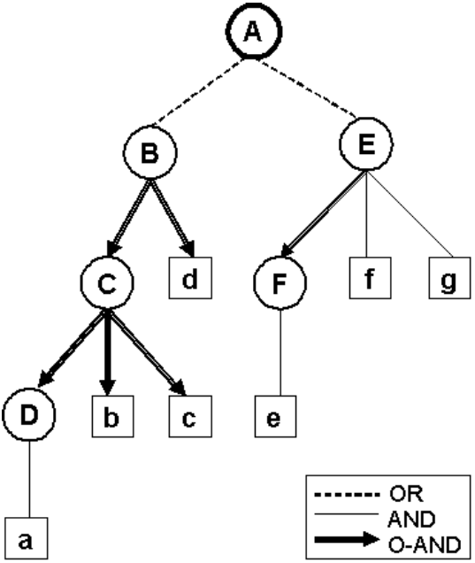
Figure 7: Enhanced attack tree for “Bypassing 802.1x” [31]

⬇

1begin attack diagram

2 A -OR-> {B, E}

3 B -OAND-> [C, d]

4 C -OAND-> [D, b, c]

5 D -AND-> {a}

6 E -OAND-> [F, fg]

7 fg -AND-> {f, g}

8 F -> {e}

9end attack diagram

Code 16: Attack tree of Fig. 7 in RisQFLan

VII-A2 Specifying Ordered Attacks in RisQFLan

Code 16 shows a model of the enhanced attack tree of Fig. 7 in RisQFLan. It is worth observing how the ordering relation is modeled. The original model in Fig. 7 prescribes that: (i) to achieve attack B, sub-goal C must be achieved before d (cf. Line 3 in Code 16); (ii) to achieve attack C, sub-goal D must be achieved before b, which itself must be achieved before c (cf. Line 4 in Code 16); and (iii) to achieve attack E, sub-goal F must be achieved before f and g (cf. Lines 6-7 in Code 16). Note that in the RisQFLan specification, auxiliary node fg is used to group the unordered conjunction of f and g.

VII-A3 Complementing the Analysis of [31] with RisQFLan

The main analysis feature of the approach in [31] consists of inspecting activity logs to recognise potential attacks as per the specified enhanced attack trees. With RisQFLan this can be augmented with exact or statistical probabilistic verification on the average behaviour of specific attacker profiles. To illustrate this we modeled four attacker profiles:

Best: an attacker that knows one of the optimal order of attacks to perform to achieve the main attack goal;

AverageA: an attacker randomly trying attacks until achieving the main attack goal or a wrong order led to failure;

AverageB: like AverageA but can undo attacks (backtrack);

Worst: like AverageA but chooses attacks with a probability inversely proportional to the order used by Best.

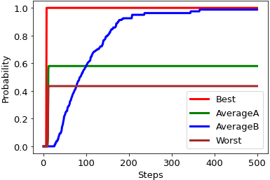
Figure 8: Statistical analysis on “Bypassing 802.1x”

Fig. 8 presents the results of SMC analysis of each such attacker profile, showing that they converge to different attack success probabilities. We have also exported the corresponding DTMCs and analysed them with PMC using PRISM. PRISM computed the same results for all attackers except for AverageB, whose DTMC is too large (due to backtracking in the attacker’s strategy) for PRISM or STORM to be able to handle it. Attackers Best and AverageB obviously achieve the attack with probability 1, although the latter needs more time. The AverageA attacker is next, achieving a success probability slightly above $0.6$, while the Worst attacker achieves an attack with probability about $0.4$.

VII-B Case Study 2: Noticeability

This section shows that the RisQFLan DSL can be used to model features from capabilities-based attack trees [35], an extension of basic attack trees offered in the commercial attack tree-based risk assessment tool SecurITree [24]. This means RisQFLan complements the models of SecurITree with explicit dynamic attack behavior  and its analysis capabilities with analysis of attacker profiles. We illustrate how the notion of noticeability, one of the capability features of capabilities-based attack trees, can be specified in RisQFLan.

VII-B1 Noticeability Capabilities of BurgleHouse

As illustrative example, we use two attack scenarios studied in [24], namely the Cat Burglar and Juvenile Delinquent scenarios from the BurgleHouse case study. Fig. 9, reproduced from [24], depicts two capabilities-based attack trees which can be easily encoded in the RisQFlan DSL using OR and AND refinements. The idea is that a house can be burglarized by entering the house by carrying out two sub-goals: WalkUpToHouse and PenetrateHouse. The latter is further refined into sub-goals. In the Cat Burglar scenario the house can only be penetrated via a GarageAttack, whereas in the Juvenile Delinquent scenario there are two further alternatives: opening the passage door by breaking it down or entering via the window by breaking the glass. We consider one of the three so-called behavioral indicators associated to attacker actions in [24], namely noticeability. The values were kindly provided by Terry Ingoldsby of Amenaza Technologies Ltd. together with a license for SecurITree v5.0.

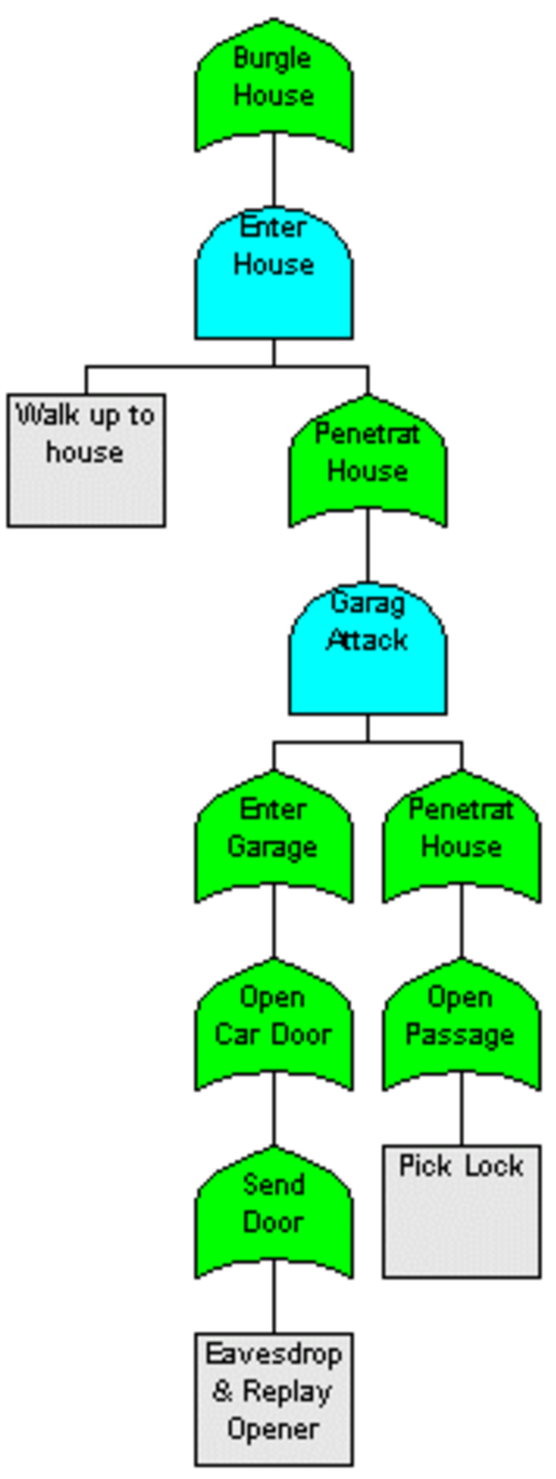
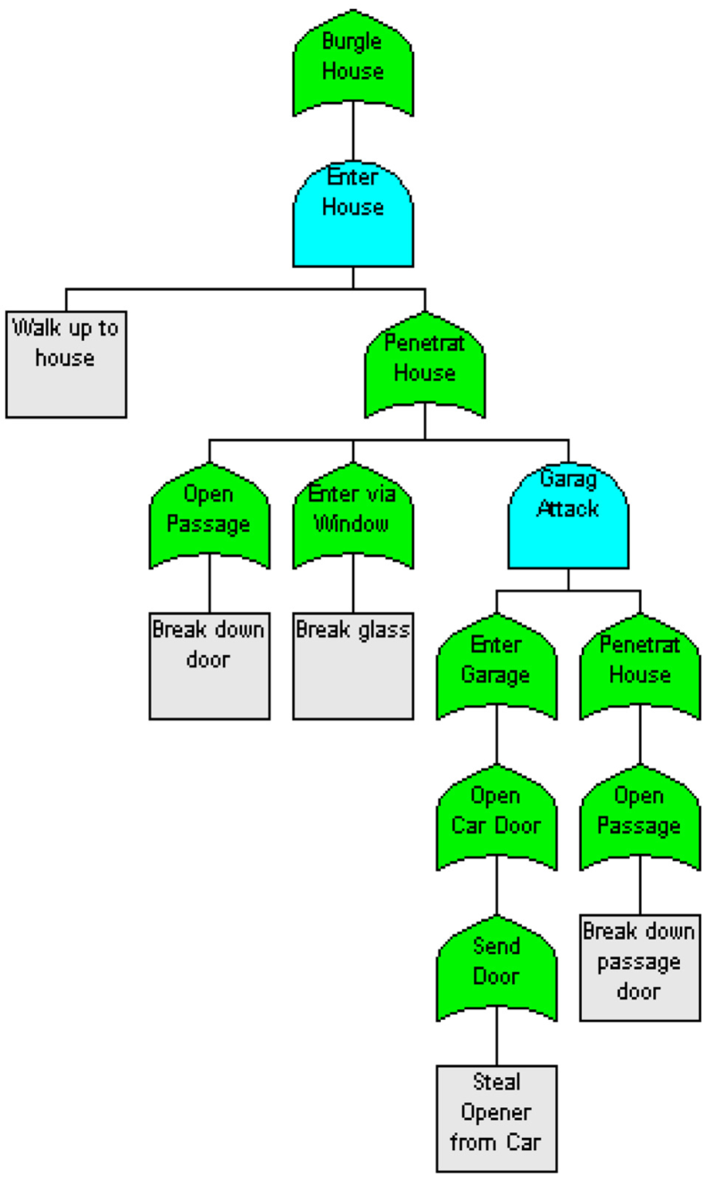
Figure 9: Capabilities-based attack trees: “Cat Burglar” (left) and “Juvenile Delinquent” (right) [24]

VII-B2 Noticeability in RisQFLan

Codes 17 and 18 show how the noticeability values of the Cat Burglar and Juvenile Delinquent scenarios, resp., are modeled as a Noticeability attribute in RisQFLan: walking up to the house is almost unnoticeable, while breaking a door or glass is more noticeable.

⬇

1begin attributes

2 Noticeability = {WalkUpToHouse = 0.01,

3 EavesdropAndReplayOpenerCode = 0.05, PickLock = 0.02}

4end attributes

Code 17: Noticeability of “Cat Burglar” specified in RisQFLan

⬇

1begin attributes

2 Noticeability = {WalkUpToHouse = 0.01,

3 BreakDownDoor = 0.3, BreakGlass = 0.3,

4 StealOpenerFromCar = 0.2, BreakDownPassageDoor = 0.1}

5end attributes

Code 18: Noticeability of “Juvenile Delinquent” in RisQFLan

VII-B3 Complementing the Analysis of [24] with RisQFLan

One of the analysis features of SecurITree consists of the possibility to identify attack scenarios according to one or more behavioral indicators. For instance, by pruning the complete attack tree of the BurgleHouse case study with $29$ nodes, SecurITree identified the above scenarios as corresponding to the specific capabilities of threat agents of the Cat Burglar and Juvenile Delinquent type (which avoid attacks that involve a risk of getting caught greater than 10% and 30%, resp., expressed through the noticeability criterion). Similarly, RisQFLan can limit its analysis to such type of scenarios by imposing quantitative constraints (cf. Code 10 in Section IV). However, RisQFLan can also augment such analyses with quantitative verification on the average behavior of specific attacker profiles as well as with estimation of the average noticeability of specific (successful) attacks. To illustrate this, we modeled four attacker profiles:

Best: an attacker that knows an optimal, most unnoticeable order of attacks to perform to achieve the main attack goal;

AverageA: an attacker that randomly tries attacks until the main attack goal is achieved;

AverageB: like AverageA but can undo attacks (backtrack);

Worst: like AverageA but chooses attacks with a probability inversely proportional to Best.

We analysed these 4 attackers in the two scenarios using the SMC analysis capabilities of RisQFLan. Fig. 10 and Fig. 11 show how the attacker profiles converge to different average noticeability values of the attacks . Note that, contrary to the case study presented in the previous section, none of the orders of attacks can result in failure. In fact, while not shown, in both scenarios all attackers succeed with probability $1$, although in both cases attacker AverageB needs considerably more time. Moreover, in the Cat Burglar scenario, all successful attackers that cannot backtrack use the same set of actions. In fact, the average noticeability value of the Best, AverageA, and Worst attackers is $8$, whereas the repeated attack attempts of the AverageB attacker guarantee that (s)he will be noticed.

However, in the Juvenile Delinquent scenario, even successful attackers may have made use of different sets of actions, due to the three different ways to penetrate the house (PenetrateHouse -OR-> {OpenPassageDoor, EnterViaWindow, GarageAttack}). In fact, the average noticeability value of the Best attacker is just over $3$, that of the AverageA and Worst attackers is just over $9$, while also in this case the repeated attack attempts of the AverageB attacker guarantee that (s)he will be noticed.

RisQFLan thus allows to analyze the risk of getting caught for different types of behavior of a concrete Cat Burglar or Juvenile Delinquent and to estimate who runs less risk. SecurITree considers such explicit dynamic attack behavior in a slightly different way. It offers advanced analysis functionalities to estimate the risk of scenarios by combining the impact of attacks and the so-called capabilistic attack propensity, which is expressed by considering feasibility (e.g. cost or resources) vs. benefits (rewards) and detriments incurred in attacks.

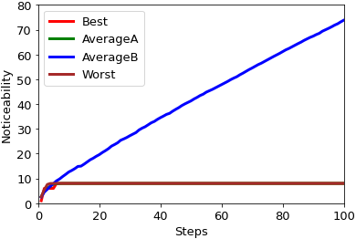
Figure 10: Statistical analysis on “Cat Burglar”

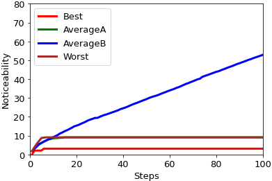
Figure 11: Statistical analysis on “Juvenile Delinquent”

VII-C Case Study 3: Countermeasures

As in the previous sections, we focus on an influential approach to attack trees, attack countermeasure trees [33], which has inspired some of RisQFLan’s modeling features. We show how RisQFLan DSL can specify the novel reactive defense mechanisms that were introduced in attack countermeasure trees, namely detection events that model defensive mechanisms to detect that an attack is being attempted and measure events that model defensive mechanisms to mitigate the effect of an attack.

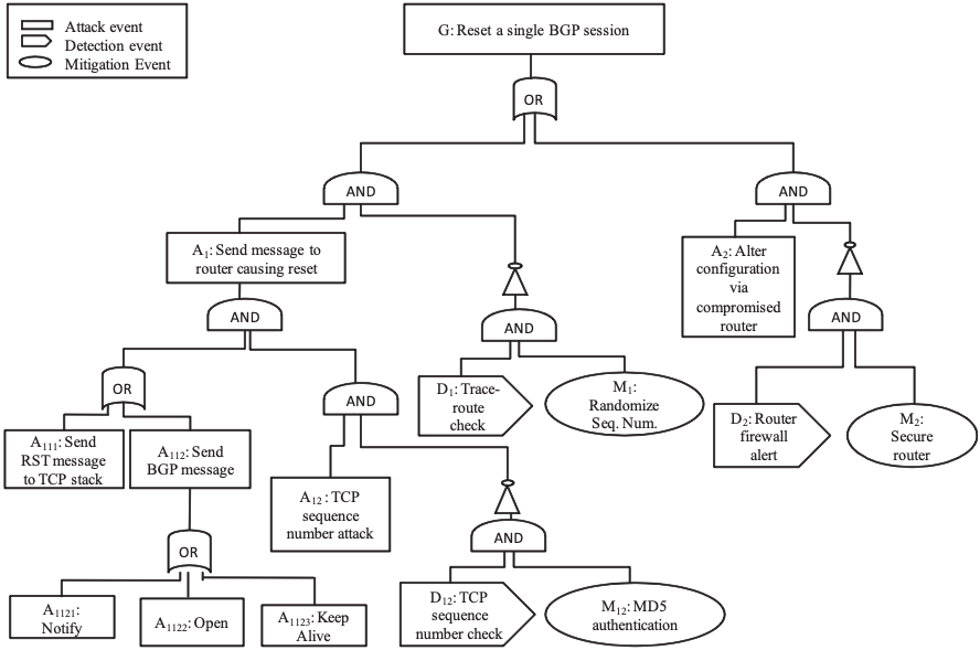
Figure 12: Countermeasure tree for “Resetting BGP” [33]

VII-C1 Countermeasures Against “Resetting BGP”

As illustrative example, we use a case study from [33], namely an attack countermeasure tree modeling defensive mechanisms against resetting attacks on the so-called Border Gateway Protocol (BGP). Fig. 12, reproduced from [33], depicts the attack countermeasure tree for this scenario. The idea is to model a known denial-of-service attack on the BGP: the attacker tries to reset a BGP session again and again to prevent communication. Such attacks consist of several steps, some of which can be detected and mitigated with well-known techniques (e.g. TCP sequence number attacks (A12) can be detected with TCP sequence number checks (D12), and a mitigation mechanism for such attacks is using MD5 authentication (M12)).

VII-C2 Countermeasures in RisQFLan

Code 19 shows how to model the attack countermeasure tree of Fig. 12 in RisQFLan.

In particular, we remark the following:

• detection events D12, D1 and D2 are modeled as countermeasure nodes; the attacks A12, A1 and A2 they intend to detect, resp., are specified accordingly (cf. Line 9 in Code 19);

• measure events M12, M1 and DM2 are modeled as defense nodes (cf. Line 5 in Code 19); the attacks A12, A1 and A2 they mitigate, resp., are specified as attack effectiveness block (cf. Line 27 in Code 19);

• the relation between a detection event D and its triggered mitigation event M is modeled in RisQFLan by specifying defense node D as a refinement of countermeasure node M (cf. Lines 18-20 in Code 19).

⬇

1begin attack nodes

2 G A1 A111 A112 A1121 A1122 A1123 A12 A2 OR1

3end attack nodes

4

5begin defense nodes

6 M12 M1 M2

7end defense nodes

8

9begin countermeasure nodes

10 D12 = {A12}, D1 = {A1}, D2 = {A2}

11end countermeasure nodes

12

13begin attack diagram

14 G -OR-> {A1, A2}

15 A1 -AND-> {OR1, A12}

16 OR1 -OR-> {A111, A112}

17 A112 -OR->{A1121,A1122,A1123}

18 D12 -AND-> {M12}

19 D1 -AND-> {M1}

20 D2 -AND-> {M2}

21end attack diagram

22

23begin attack detection rates

24 A1 = 0.5, A12 = 0.5, A2 = 0.5

25end attack detection rates

26

27begin defense effectiveness

28 M12(ALL, A12) = 0.5, M1(ALL, A1) = 0.5, M2(ALL, A2) = 0.5

29end defense effectiveness

Code 19: Fig. 12 in RisQFLan

VII-C3 Complementing the Analysis of [33] with RisQFLan

The approach in [33] includes rich analyses for attack countermeasure trees, including success probabilities, costs and impact of attacks and defensive mechanisms. RisQFLan can augment such analyses with quantitative verification of specific attacker profiles. To illustrate this, we modeled three profiles:

Random: an attacker that randomly tries attacks until the main attack goal is achieved;

Noisy: like Random but tries attacks for which countermeasures exist with higher probability with respect to those for which no countermeasure exists;

Sneaky: like Random but tries attacks for which countermeasures exist with lower probability with respect to those for which no countermeasure exists.

We analysed this scenario using the PMC functionalities of PRISM. Indeed, the DMTCs for the attackers could be generated by RisQFLan, and handled by PRISM. We labeled with hasG all states when has(G) was satisfied. The property we studied is the probability of success at each step, suitably formulated in the property specification language of PRISM. Fig. 13, generated by PRISM, shows the results of the analyses: since all attackers are given the chance to try again and again, they are all eventually successful, but they differ with respect to the amount of time needed to succeed. Paradoxically, the Noisy attacker converges faster, which means that the detection and measure events are not as effective as they should be.

\begin{overpic}[width=433.62pt]{figures/bgp-prism-plot.pdf} \put(80.0,10.0){\includegraphics[width=65.04034pt]{figures/bgp-prism-legend.pdf}} \end{overpic}

Figure 13: Exact PMC analysis on “Resetting BGP”

VIII Related Work

There is a large body of related work. Throughout the paper, we indicated some sources of inspiration, like attack profiles specified as automata to describe possible attack steps and their costs [13, 51] and the attack detection rates [24], ordered attacks [31] and countermeasures [33] treated in Sections VII-A, VII-B and VII-C, resp. A recent study by Wideł et al. [23] classified existing approaches integrating attack tree-based modeling and formal methods along three dimensions. We believe that RisQFLan can act as a unification of those dimensions. In this section, we detail the dimensions and relate RisQFLan to existing approaches.

The first dimension (a major focus of the large-scale EU project TRESPASS [52]) is the generation of attack trees from scenarios. The main difficulty is to find a compact and effective representation, knowing that structurally different trees can capture the same information. A representative contribution in this area is the ATSyRa toolset [53]. An original and crucial feature of ATSyRa is the support for high-level actions (which can be seen as a sub-goal of the attacker) to specify how sequences of actions can be abstracted and structured. Those high-level actions can later be used in a refactorization and hence better representation of the tree. The contribution is packed up in an elegant Eclipse plugin which makes it easily accessible to the uninitiated. Another contribution is the process-algebraic generation approach from Vigo and the Nielsons [54], where attacks are generated from flow constraints using a SAT solver, and a value-passing quality calculus is used to represent how an attacker can reach a given location. Our approach is not concerned with the synthesis of attack trees, but those techniques and tools could be combined in RisQFLan, to complement them with analysis capabilities.

The second dimension in [23] is that of giving a rigorous mathematical meaning to (extended) attack trees. The objective is to address a wide range of static problems, like comparing trees or enumerating the attacks. Well-known representations include Boolean function-based semantics, multisets, and linear logics (cf. [23, 55] and their references). This research trend is very similar to the one applied to feature diagrams [56], and it is likely that many results from the software engineering community concerning product lines or configurable systems can be transferred to the security domain [57]. It is worth noticing that the above mentioned approaches do not permit reasoning on the order of steps of the attack, a distinguishing feature that our approach has adopted, together with the ability to undo attack action.

More recently, several researchers have suggested to extend attack tree representations with their environment, i.e. the attacker and the system under attack. For example, the authors of [14, 15] not only consider the attack tree itself, but also a transition system representation of an attacker model. The separation of the attack tree from the attacker model as we do in RisQFLan is fundamental to avoid confusion as explained by Mantel et al. [58]. This addition allows one to reason not only on static problems, but also on dynamic ones. For instance, one can make hypotheses on attack step sequences or extract correlations between step orders. In addition, the use of transition system-based representations allows one to encompass a model of the system under attack, and by consequences of (the order of) its defenses [59]. In this context, contributions like [14] consider that defenses are fixed a priori, while the game-based approach of Aslanyan et al. [5] allows one to propose them dynamically to react to specific orders of attack steps. Observe that the latter proposal generalizes the sequential conjunction approach of Jhawar et al. [60]. RisQFLan follows the approach of Aslanyan et al., but uses SMC [12] (in addition to exact PMC), a simulation-based approach that is less precise but more effective than the exhaustive state-space exploration of the game-based approach. Moreover, RisQFLan offers a richer language to express constraints between attack steps and the behavior of the system under attack.

The third dimension proposed in [23] is that of adding quantitative algorithms to reason on (extensions of) attack trees. This is achieved by enriching attack trees with quantitative information, like the cost or probability of an attack step. In this context, static techniques can still be used to answer extended membership queries such as computing the cost of an attack, the Pareto optimal attack for two or more quantitative parameters, or the optimal countermeasures [61, 62, 63]. However, as observed by Kordy et al., minimal representations no longer exist [34, 64], which drastically complicates both the comparison and the synthesis of trees. Quantitative analysis extends to the dynamic case, meaning one can benefit from all the recent work on quantitative formal verification, where the attacker model can remain non-deterministic or even become stochastic. One can then synthesize strategies of the attacker that belongs to the tree and for which the cost is at most a certain value. Over the last five years, a wide range of such techniques has been proposed. Some of those techniques were developed by Legay et al. [14, 15]. These approaches rely on a quantitative representation of the attacker together with a timed automata-based model for the system. Defenses are provided a priori. The approaches were implemented in the UPPAAL framework, which allows one to use extensions like UPPAAL SMC [65] to compute the probability or cost of an attack. In case non-determinism is added to the attacker model, UPPAAL Stratego [66] can be used to synthesize strategies.

RisQFLan goes further than [14, 15] by (i) proposing a DSL and (ii) allowing to not only quantify the number of attack steps, but also offering a rich process-algebraic language to impose conditions between steps as well as between defenses that can moreover be added at runtime. However, RisQFLan does not offer non-determinism for attackers. This may be needed to reason on the use of several strategies. A solution could be to add non-deterministic aspects to the DSL, and extend our DTMC exporter to an exporter for Markov decision processes, or in the input language of UPPAAL if also time aspects were to be considered, or to combine RisQFLan’s SMC engine with the Plasma Plugin for non-deterministic systems [67]. The approach by Aslanyan et al. [5] allows reasoning on causality between steps and non-deterministic attackers, but restricted to Boolean causalities called waves, and without DSL. Stoelinga et al. also proposed dynamic approaches to analyze attack trees via SMC. Those approaches are covered and extended by RisQFLan, especially concerning (i) the causality part and (ii) the DSL, which is restricted to the query part with LOCKS [68]. Finally, compared to the three approaches mentioned above, only RisQFLan proposes a fully dedicated and maintained open-source toolset.

IX Conclusion and Future Work

We instantiated QFLan in the quantitative security risk modeling and analysis domain, and applied the outcome, RisQFLan, to 3 case studies from well-known tools from the graph-based risk modeling and analysis domain. By enhancing the analysis features of these tools with either exact or statistical verification of probabilistic attack scenarios, RisQFLan constitutes a significant contribution to the domain’s toolsets.

The generalization and subsequent instantiation of QFLan was feasible since it is open source, a distinguishing feature of RisQFLan among the toolsets available in the domain. RisQFLan’s DTMC exporting facilities moreover permit tool-chaining with probabilistic model checkers for models of sizes that do not require SMC.

RisQFLan could be further enriched in several directions. First, we propagate the value of an attribute of a node as the sum of the attribute’s values of its descendants. This could be generalized to attribute-specific formulae as in SecurITree, in which, e.g., the noticeability value of a node with $n$ descendants $d_{1},d_{2},\ldots,d_{n}$ is computed as $1-((1-d_{1})(1-d_{2})\cdots(1-d_{n}))$. Most properties analysed so far with RisQFLan concern logical requirements. Recently, SMC has also been used to compare system behavior via simulation [69]. We could compare the behavior of two attackers via simulation or their effect on two different attack-defense diagrams.

We also plan to consider non-deterministic and game aspects along the lines of [5, 14, 15], as discussed in detail in Section VIII, as well as synthesis of attack profiles and countermeasures (cf., e.g., [63]) for underspecified attack profiles.

References

- [1] M. Bozga, A. David, A. Hartmanns, H. Hermanns, K. G. Larsen, A. Legay, and J. Tretmans, “State-of-the-Art Tools and Techniques for Quantitative Modeling and Analysis of Embedded Systems,” in Proceedings of the Conference on Design, Automation and Test in Europe (DATE’12). EDAA, 2012, pp. 370–375.
- [2] J. Katoen and K. G. Larsen, “Quantitative Modelling and Analysis,” in Proceedings of the 5th International Symposium on Leveraging Applications of Formal Methods, Verification and Validation: Applications and Case Studies (ISoLA’12), ser. Lecture Notes in Computer Science, T. Margaria and B. Steffen, Eds., vol. 7610. Springer, 2012, pp. 290–292.
- [3] A. Hartmanns and H. Hermanns, “In the quantitative automata zoo,” Sci. Comput. Program., vol. 112, pp. 3–23, 2015.
- [4] R. Kumar, E. Ruijters, and M. Stoelinga, “Quantitative Attack Tree Analysis via Priced Timed Automata,” in Proceedings of the 13th International Conference on Formal Modeling and Analysis of Timed Systems (FORMATS’15), ser. Lecture Notes in Computer Science, S. Sankaranarayanan and E. Vicario, Eds., vol. 9268. Springer, 2015, pp. 156–171.
- [5] Z. Aslanyan, F. Nielson, and D. Parker, “Quantitative Verification and Synthesis of Attack-Defence Scenarios,” in Proceedings of the IEEE 29th Computer Security Foundations Symposium (CSF’16). IEEE, 2016, pp. 105–119.
- [6] M. Bernardo, R. De Nicola, and J. Hillston, Eds., Formal Methods for the Quantitative Evaluation of Collective Adaptive Systems, ser. Lecture Notes in Computer Science, vol. 9700. Springer, 2016.
- [7] R. Kumar and M. Stoelinga, “Quantitative Security and Safety Analysis with Attack-Fault Trees,” in Proceedings of the 18th IEEE International Symposium on High Assurance Systems Engineering (HASE’17). IEEE, 2017, pp. 25–32.
- [8] M. H. ter Beek, A. Legay, A. Lluch Lafuente, and A. Vandin, “A framework for quantitative modeling and analysis of highly (re)configurable systems,” IEEE Trans. Softw. Eng., vol. 46, no. 3, pp. 321–345, 2020.
- [9] M. H. ter Beek and A. Legay, “Quantitative variability modelling and analysis,” Int. J. Softw. Tools Technol. Transf., vol. 21, no. 6, pp. 607–612, 2019.
- [10] E. M. Hahn, A. Hartmanns, C. Hensel, M. Klauck, J. Klein, J. Kretínský, D. Parker, T. Quatmann, E. Ruijters, and M. Steinmetz, “The 2019 comparison of tools for the analysis of quantitative formal models,” in Proceedings of the 25th International Conference on Tools and Algorithms for the Construction and Analysis of Systems: TOOLympics (TACAS’19), ser. Lecture Notes in Computer Science, D. Beyer, M. Huisman, F. Kordon, and B. Steffen, Eds., vol. 11429. Springer, 2019, pp. 69–92.
- [11] G. Agha and K. Palmskog, “A survey of statistical model checking,” ACM Trans. Model. Comp. Simul., vol. 28, no. 1, pp. 6:1–6:39, 2018.
- [12] A. Legay, A. Lukina, L. Traonouez, J. Yang, S. A. Smolka, and R. Grosu, “Statistical Model Checking,” in Computing and Software Science: State of the Art and Perspectives, ser. Lecture Notes in Computer Science, B. Steffen and G. J. Woeginger, Eds. Springer, 2019, vol. 10000, pp. 478–504.
- [13] A. Lenin, J. Willemson, and D. P. Sari, “Attacker Profiling in Quantitative Security Assessment Based on Attack Trees,” in Proceedings of the 19th Nordic Conference on Secure IT Systems (NordSec’14), ser. Lecture Notes in Computer Science, K. Bernsmed and S. Fischer-Hübner, Eds., vol. 8788. Springer, 2014, pp. 199–212.
- [14] O. Gadyatskaya, R. R. Hansen, K. G. Larsen, A. Legay, M. C. Olesen, and D. B. Poulsen, “Modelling Attack-defense Trees Using Timed Automata,” in Proceedings of the 14th International Conference on Formal Modeling and Analysis of Timed Systems (FORMATS’16), ser. Lecture Notes in Computer Science, M. Fränzle and N. Markey, Eds., vol. 9884. Springer, 2016, pp. 35–50.
- [15] R. R. Hansen, P. G. Jensen, K. G. Larsen, A. Legay, and D. B. Poulsen, “Quantitative Evaluation of Attack Defense Trees Using Stochastic Timed Automata,” in Proceedings of the 4th International Workshop on Graphical Models for Security (GraMSec’17), ser. Lecture Notes in Computer Science, P. Liu, S. Mauw, and K. Stølen, Eds., vol. 10744. Springer, 2017, pp. 75–90.
- [16] R. Kumar, S. Schivo, E. Ruijters, B. M. Yildiz, D. Huistra, J. Brandt, A. Rensink, and M. Stoelinga, “Effective Analysis of Attack Trees: A Model-Driven Approach,” in Proceedings of the 21st International Conference on Fundamental Approaches to Software Engineering (FASE’18), ser. Lecture Notes in Computer Science, A. Russo and A. Schürr, Eds., vol. 10802. Springer, 2018, pp. 56–73.
- [17] E. M. Clarke, T. A. Henzinger, H. Veith, and R. Bloem, Eds., Handbook of Model Checking. Springer, 2018.
- [18] B. Schneier, “Attack trees,” Dr. Dobb’s Journal, 1999. [Online]. Available: https://www.schneier.com/academic/archives/1999/12/attack_trees.html
- [19] S. Mauw and M. Oostdijk, “Foundations of Attack Trees,” in Proceedings of the 8th International Conference on Information Security and Cryptology (ICISC’05), ser. Lecture Notes in Computer Science, D. Won and S. Kim, Eds., vol. 3935. Springer, 2005, pp. 186–198.
- [20] B. Kordy, S. Mauw, S. Radomirović, and P. Schweitzer, “Foundations of Attack-Defense Trees,” in Proceedings of the 7th International Workshop on Formal Aspects in Security and Trust (FAST’10), ser. Lecture Notes in Computer Science, P. Degano, S. Etalle, and J. Guttman, Eds., vol. 6561. Springer, 2011, pp. 80–95.
- [21] B. Kordy, L. Piètre-Cambacédès, and P. Schweitzer, “DAG-based attack and defense modeling: Don’t miss the forest for the attack trees,” Comput. Sci. Rev., vol. 13–14, pp. 1–38, 2014.
- [22] J. B. Hong, D. S. Kim, C. Chung, and D. Huang, “A survey on the usability and practical applications of Graphical Security Models,” Comput. Sci. Rev., vol. 26, pp. 1–16, 2017.
- [23] W. Wideł, M. Audinot, B. Fila, and S. Pinchinat, “Beyond 2014: Formal Methods for Attack Tree–Based Security Modeling,” ACM Comput. Surv., vol. 52, no. 4, pp. 75:1–75:36, 2019.
- [24] Amenaza Technologies Limited, The SecuITree® BurgleHouse Tutorial (a.k.a., Who wants to be a Cat Burglar?), 2nd ed., 2006, (cf. [35]). [Online]. Available: https://www.amenaza.com/downloads/docs/Tutorial.pdf
- [25] B. Kordy, P. Kordy, S. Mauw, and P. Schweitzer, “ADTool: Security Analysis with Attack–Defense Trees,” in Proceedings of the 10th International Conference on Quantitative Evaluation of Systems (QEST’13), ser. Lecture Notes in Computer Science, K. Joshi, M. Siegle, M. Stoelinga, and P. R. D’Argenio, Eds., vol. 8054. Springer, 2013, pp. 173–176.
- [26] B. Kordy, P. Kordy, and Y. van den Boom, “SPTool – Equivalence Checker for SAND Attack Trees,” in Proceedings of the 11th International Conference on Risks and Security of Internet and Systems (CRiSIS’16), ser. Lecture Notes in Computer Science, F. Cuppens, N. Cuppens, J. Lanet, and A. Legay, Eds., vol. 10158. Springer, 2016, pp. 105–113.
- [27] S. Sebastio and A. Vandin, “MultiVeStA: Statistical Model Checking for Discrete Event Simulators,” in Proceedings of the 7th International Conference on Performance Evaluation Methodologies and Tools (ValueTools’13). ACM, 2013, pp. 310–315.
- [28] S. Gilmore, D. Reijsbergen, and A. Vandin, “Transient and Steady-State Statistical Analysis for Discrete Event Simulators,” in Proceedings of the 13th International Conference on Integrated Formal Methods (IFM’17), ser. Lecture Notes in Computer Science, N. Polikarpova and S. Schneider, Eds., vol. 10510. Springer, 2017, pp. 145–160.
- [29] M. Z. Kwiatkowska, G. Norman, and D. Parker, “PRISM 4.0: Verification of Probabilistic Real-Time Systems,” in CAV, ser. Lecture Notes in Computer Science, G. Gopalakrishnan and S. Qadeer, Eds., vol. 6806. Springer, 2011, pp. 585–591.
- [30] C. Dehnert, S. Junges, J. Katoen, and M. Volk, “A Storm is Coming: A Modern Probabilistic Model Checker,” in CAV, ser. Lecture Notes in Computer Science, R. Majumdar and V. Kunčak, Eds., vol. 10427. Springer, 2017, pp. 592–600.
- [31] S. A. Çamtepe and B. Yener, “Modeling and detection of complex attacks,” in Proceedings of the 3rd International Conference on Security and Privacy in Communication Networks (SecureComm’07). IEEE, 2007, pp. 234–243.
- [32] W. Lv and W. Li, “Space Based Information System Security Risk Evaluation Based on Improved Attack Trees,” in Proceedings of the 3rd International Conference on Multimedia Information Networking and Security (MINES’11). IEEE, 2011, pp. 480–483.
- [33] A. Roy, D. S. Kim, and K. S. Trivedi, “Attack countermeasure trees (ACT): towards unifying the constructs of attack and defense trees,” Secur. Commun. Netw., vol. 5, no. 8, pp. 929–943, 2012.
- [34] B. Kordy, S. Mauw, and P. Schweitzer, “Quantitative Questions on Attack-Defense Trees,” in Proceedings of the 15th International Conference on Information Security and Cryptology (ICISC’12), ser. Lecture Notes in Computer Science, T. Kwon, M. Lee, and D. Kwon, Eds., vol. 7839. Springer, 2012, pp. 49–64.
- [35] T. R. Ingoldsby, “Attack Tree-based Threat Risk Analysis,” Amenaza Technologies Limited, Tech. Rep., October 2013. [Online]. Available: https://www.amenaza.com/downloads/docs/AttackTreeThreatRiskAnalysis.pdf
- [36] A. Vandin, M. H. ter Beek, A. Legay, and A. Lluch Lafuente, “QFLan: A Tool for the Quantitative Analysis of Highly Reconfigurable Systems,” in Proceedings of the 22nd International Symposium on Formal Methods (FM’18), ser. Lecture Notes in Computer Science, K. Havelund, J. Peleska, B. Roscoe, and E. de Vink, Eds., vol. 10951. Springer, 2018, pp. 329–337.
- [37] C. Baier and J.-P. Katoen, Principles of Model Checking. The MIT Press, 2008. [Online]. Available: http://mitpress.mit.edu/books/principles-model-checking
- [38] S. Gilmore, M. Tribastone, and A. Vandin, “An Analysis Pathway for the Quantitative Evaluation of Public Transport Systems,” in Proceedings of the 11th International Conference on Integrated Formal Methods (IFM’14), ser. Lecture Notes in Computer Science, E. Albert and E. Sekerinski, Eds., vol. 8739. Springer, 2014, pp. 71–86.
- [39] M. H. ter Beek, A. Legay, A. Lluch Lafuente, and A. Vandin, “Statistical Model Checking for Product Lines,” in Proceedings of the 7th International Symposium on Leveraging Applications of Formal Methods, Verification and Validation: Foundational Techniques (ISoLA’16), ser. Lecture Notes in Computer Science, T. Margaria and B. Steffen, Eds., vol. 9952. Springer, 2016, pp. 114–133.
- [40] P. Filipovikj, N. Mahmud, R. Marinescu, C. Seceleanu, O. Ljungkrantz, and H. Lönn, “Simulink to UPPAAL Statistical Model Checker: Analyzing Automotive Industrial Systems,” in FM, ser. LNCS, J. Fitzgerald, C. Heitmeyer, S. Gnesi, and A. Philippou, Eds., vol. 9995. Springer, 2016, pp. 748–756.
- [41] A. Arnold, M. Baleani, A. Ferrari, M. Marazza, V. Senni, A. Legay, J. Quilbeuf, and C. Etzien, “An Application of SMC to continuous validation of heterogeneous systems,” EAI Endorsed Trans. Indust. Netw. & Intellig. Syst., vol. 4, no. 10, 2017.
- [42] D. Basile, F. Di Giandomenico, and S. Gnesi, “Statistical Model Checking of an Energy-Saving Cyber-Physical System in the Railway Domain,” in Proceedings 32nd Symposium on Applied Computing (SAC). ACM, 2017, pp. 1356–1363.
- [43] Q. Cappart, C. Limbrée, P. Schaus, J. Quilbeuf, L. Traonouez, and A. Legay, “Verification of Interlocking Systems Using Statistical Model Checking,” in Proceedings of the 18th International Symposium on High Assurance Systems Engineering (HASE’17). IEEE, 2017, pp. 61–68.
- [44] D. Basile, M. H. ter Beek, and V. Ciancia, “Statistical Model Checking of a Moving Block Railway Signalling Scenario with Uppaal SMC,” in ISoLA, ser. LNCS, T. Margaria and B. Steffen, Eds., vol. 11245. Springer, 2018, pp. 372–391.
- [45] S. Puch, M. Fränzle, and S. Gerwinn, “Quantitative Risk Assessment of Safety-Critical Systems via Guided Simulation for Rare Events,” in ISoLA, ser. LNCS, T. Margaria and B. Steffen, Eds., vol. 11245. Springer, 2018, pp. 305–321.
- [46] R. Bao, J. C. Attiogbé, B. Delahaye, P. Fournier, and D. Lime, “Parametric Statistical Model Checking of UAV Flight Plan,” in FORTE, ser. LNCS, J. A. Pérez and N. Yoshida, Eds., vol. 11535. Springer, 2019, pp. 57–74.
- [47] D. Basile, M. H. ter Beek, A. Ferrari, and A. Legay, “Modelling and Analysing ERTMS L3 Moving Block Railway Signalling with Simulink and UPPAAL SMC,” in FMICS, ser. LNCS, K. G. Larsen and T. Willemse, Eds., vol. 11687. Springer, 2019, pp. 1–21.
- [48] D. Basile, A. Fantechi, L. Rucher, and G. Mandò, “Statistical model checking of hazards in an autonomous tramway positioning system,” in RSSRail, ser. LNCS, S. Collart-Dutilleul, T. Lecomte, and A. B. Romanovsky, Eds., vol. 11495. Springer, 2019, pp. 41–58.
- [49] A. Ferrari, F. Mazzanti, D. Basile, M. H. ter Beek, and A. Fantechi, “Comparing Formal Tools for System Design: a Judgment Study,” in Proceedings 42nd International Conference on Software Engineering (ICSE). ACM, 2020.
- [50] H. Garavel, M. H. ter Beek, and J. van de Pol, “The 2020 Expert Survey on Formal Methods,” in FMICS, ser. LNCS, M. ter Beek and D. Ničković, Eds., vol. 12327. Springer, 2020, pp. 3–69.
- [51] H. Hermanns, J. Krämer, J. Krcál, and M. Stoelinga, “The Value of Attack-Defence Diagrams,” in Proceedings of the 5th International Conference on Principles of Security and Trust (POST’16), ser. Lecture Notes in Computer Science, F. Piessens and L. Viganò, Eds., vol. 9635. Springer, 2016, pp. 163–185.
- [52] “H2020 project on robusT Risk basEd Screening and alert System for PASSengers and luggage.” [Online]. Available: https://www.tresspass.eu/The-project
- [53] S. Pinchinat, M. Acher, and D. Vojtisek, “ATSyRa: An Integrated Environment for Synthesizing Attack Trees - (Tool Paper),” in Proceedings of the 2nd International Workshop on Graphical Models for Security (GraMSec’15), ser. Lecture Notes in Computer Science, S. Mauw, B. Kordy, and S. Jajodia, Eds., vol. 9390. Springer, 2015, pp. 97–101.
- [54] R. Vigo, F. Nielson, and H. R. Nielson, “Automated generation of attack trees,” in Proceedings of the 27th IEEE Computer Security Foundations Symposium (CSF’14). IEEE, 2014, pp. 337–350.
- [55] M. Audinot, S. Pinchinat, and B. Kordy, “Is My Attack Tree Correct?” in Proceedings 22nd European Symposium on Research in Computer Security (ESORICS’17), ser. Lecture Notes in Computer Science, S. N. Foley, D. Gollmann, and E. Snekkenes, Eds., vol. 10492. Springer, 2017, pp. 83–102.
- [56] K. Czarnecki, S. She, and A. Wasowski, “Sample Spaces and Feature Models: There and Back Again,” in Proceedings of the 12th International Software Product Lines Conference (SPLC’08). IEEE, 2008, pp. 22–31.
- [57] M. H. ter Beek, A. Legay, A. Lluch Lafuente, and A. Vandin, “Variability meets Security,” in Proceedings of the 14th International Working Conference on Variability Modelling of Software-intensive Systems (VaMoS’20). ACM, 2020, pp. 11:1–11:9.
- [58] H. Mantel and C. W. Probst, “On the Meaning and Purpose of Attack Trees,” in Proceedings of the 32nd IEEE Computer Security Foundations Symposium (CSF’19). IEEE, 2019, pp. 184–199.
- [59] B. Kordy, S. Mauw, S. Radomirovic, and P. Schweitzer, “Attack-defense trees,” J. Log. Comput., vol. 24, no. 1, pp. 55–87, 2014.
- [60] R. Jhawar, B. Kordy, S. Mauw, S. Radomirovic, and R. Trujillo-Rasua, “Attack Trees with Sequential Conjunction,” in Proceedings of the 30th IFIP TC 11 International Conference on ICT Systems Security and Privacy Protection (SEC’15), ser. IFIP Advances in Information and Communication Technology, H. Federrath and D. Gollmann, Eds., vol. 455. Springer, 2015, pp. 339–353.
- [61] Z. Aslanyan and F. Nielson, “Pareto Efficient Solutions of Attack-Defence Trees,” in Proceedings of the 4th International Conference on Principles of Security and Trust (POST’15), ser. Lecture Notes in Computer Science, R. Focardi and A. C. Myers, Eds., vol. 9036. Springer, 2015, pp. 95–114.
- [62] B. Fila and W. Wideł, “Efficient Attack-Defense Tree Analysis using Pareto Attribute Domains,” in Proceedings of the 32nd IEEE Computer Security Foundations Symposium (CSF’19). IEEE, 2019, pp. 200–215.
- [63] ——, “Exploiting attack-defense trees to find an optimal set of countermeasures,” in Proceedings of the 33rd IEEE Computer Security Foundations Symposium (CSF’20). IEEE, 2020, pp. 395–410.
- [64] B. Kordy, M. Pouly, and P. Schweitzer, “Probabilistic reasoning with graphical security models,” Inf. Sci., vol. 342, pp. 111–131, 2016.
- [65] A. David, K. G. Larsen, A. Legay, M. Mikucionis, and D. B. Poulsen, “Uppaal SMC tutorial,” Int. J. Softw. Tools Technol. Transf., vol. 17, no. 4, pp. 397–415, 2015.
- [66] A. David, P. G. Jensen, K. G. Larsen, M. Mikučionis, and J. H. Taankvist, “Uppaal Stratego,” in Proceedings of the 21st International Conference on Tools and Algorithms for the Construction and Analysis of Systems (TACAS’15), ser. Lecture Notes in Computer Science, C. Baier and C. Tinelli, Eds., vol. 9035. Springer, 2015, pp. 206–211.
- [67] P. D’Argenio, A. Legay, S. Sedwards, and L. Traonouez, “Smart sampling for lightweight verification of Markov decision processes,” Int. J. Softw. Tools Technol. Transf., vol. 17, no. 4, pp. 469–484, 2015.
- [68] R. Kumar, A. Rensink, and M. Stoelinga, “LOCKS: a property specification language for security goals,” in Proceedings of the 33rd Annual ACM Symposium on Applied Computing (SAC’18). ACM, 2018, pp. 1907–1915.
- [69] K. G. Larsen, A. Legay, M. Mikučionis, B. Nielsen, and U. Nyman, “Compositional Testing of Real-Time Systems,” in ModelEd, TestEd, TrustEd, ser. Lecture Notes in Computer Science, J. Katoen, R. Langerak, and A. Rensink, Eds. Springer, 2017, vol. 10500, pp. 107–124.