Axial and polar modes for the ring down of a Schwarzschild black hole with an $r$ dependent mass-function

Abstract

The axial and polar modes for the ring down of a Schwarzschild black hole are calculated, by first deriving the Regge-Wheeler and Zerilli equations, respectively, and finally applying the Asymptotic Iteration Method (AIM). We were able to reach up to 500 iterations, obtaining for the first time convergence for a wide range of large damping modes. The General Relativity (GR) and a particular version of an extended model with an $r$-dependent mass-function are compared. This mass-function allows an analytical solution for the Tortoise coordinate. The example of the mass-function corresponds to the leading correction for extended theories and serves as a starting point to treat other $r$-dependent parameter mass-functions.

1 Introduction

General Relativity (GR) is one of the best tested theories, which accounts for the observations in the solar system will and also its prediction of gravitational waves maggiore was confirmed recently abbot1 ; abbot2 . The first indirect proof of these waves stems from the 1970’s hulse , through the observation of changes in the orbital frequency of a neutron star binary. The black hole merger consists of two phases: the inspiral and the ring-down phase. For the description of the inspiral phase the result depends very much on the approximation used maggiore ; hess-2016 or on a non-linear hydro-dynamic approach rezzolla-book . For the ring-down phase the situation is ”simpler”, because only the stability of the black hole under metric perturbations has to be studied. The investigation of the ring-down phase can be traced back to S. Chandrasekhar’s book on the mathematics of black holes chandra and chandra1975a ; chandra1975b (though, not the first). The equation for the calculation of the ring-down frequencies where treated in zerilli for the polar modes and in RW for the axial modes. These equations permit to calculate the frequencies, solving the eigenvalue problem of the equation, which is much simpler than to implement a dynamical theory. There are several methods to solve these equations, as for example the so-called Asymptotic Iteration Method (AIM) ciftci2003 ; ciftci2005 , with an improved approach published in cho2012 .

For this reason, we restrict our analysis to the study of the ring-down modes only and in addition to a non-rotating star, i.e., to the Schwarzschild metric. We follow closely the method described in the book of S. Chandrasekhar chandra , Chapter 4 on the perturbations of a Schwarzschild black hole.

An interesting questions is: What changes, when a $r$-dependent mass-function $m(r)$ is used, instead of a constant mass parameter $m_{0}$? There is a $1/r^{4}$ leading order, due to the following arguments: a) $1/r^{2}$ corrections are excluded due to observations in the solar system will . b) Also $1/r^{3}$ corrections are excluded due to adjusting to the inspiral phase nielsen2018 ; nielsen2019 in the first observed gravitational event. Thus, the leading corrections are of the order $1/r^{4}$. Other corrections, as appearing in cosmological models (de Sitter), are not included but the path explained can be extended to it. It is probable that the constant mass $m_{0}$ is substituted by a function in $r$ as soon as GR is extended and, therefore, it is interesting to ask what kind of changes one can expect? Does the $1/r^{4}$ correction to the metric still lead to stable modes? Is isospectrality between axial and polar modes maintained? These are some of the motivations of this contribution. To make life easier, we will use a particular mass-function which still implies an event horizon, enabling us to extend directly, with few modifications, the calculations reported in chandra .

Another example is given in hess2009 ; book where the pseudo-complex General Relativity (pc-GR) is proposed, which adds in the vicinity of a black hole a distribution of dark energy, which is repulsive and from a certain value of the coupling constnat halts the collapse of a star, before forming an event horizon and a singularity. In all applications up to now, for practical reasons, the coupling constant is chosen such that there is still an event horizon at $r=\frac{3}{2}m_{0}$. First observable predictions are published in MNRAS2013 ; MNRAS2014 . More recent descriptions of this model can be found in highenergy ; universe ; PPNP . One reason for using this theory becomes obvious in the main body of the text: The mass-function in pc-GR stars with a $1/r^{4}$ correction and we show that it permits an analytical solution for the Tortoise coordinate, thus, it provides us with a controlled handling of the asymptotic limit of the solutions. This property helps to understand the changes in the spectrum of the Quasinormal Modes (QNM) in the ring-down phase of a black hole and its stability.

Because the mass-function is such that there is still an event-horizon, one can proceed in an analog way as in GR. The only question is how to treat the accumulation of dark energy around a black hole. The distribution defines es new vacuum and it will be shown that it only depends on the total central mass through a coupling constant, which is not changed when perturbations are included.

The paper is organized as follows: In Section 2 the Schwarzschild limit will be discussed. In Section 3 the easier to treat case of axial modes are determined and in Section 4 the polar modes. In Section 5 the Regge-Wheeler and Zerilli equations are derived and the numerical method to solve the differential equation is shortly explained. In Section 6 the asymptotic limit of the corresponding solution is calculated, using an analytical solution for the Tortoise coordinate. The spectrum of axial and polar modes are determined, within GR and its extension. We will show that the isospectral symmetry observed in GR, namely that the frequencies of the axial and polar modes are the same, is not maintained for an $r$-dependent mass-function, though, some similar structures are present. In Section 7 the Conclusions are drawn.

2 The Schwarzschild solution

Following the notation of chandra ; chandra1975a ; chandra1975b , the length element is given by

$$ds^{2} = e^{2\nu}(dt)^{2}-e^{2\psi}\left(d\phi-\omega dt-q_{2}dx_{2}-q_{3}dx_{3}\right)^{2}$$ (1)

$$-e^{2\mu_{2}}(dx_{2})^{2}-e^{2\mu_{3}}(dx_{3})^{2}~{}~{}~{},$$

where $dx_{2}=r$ and $dx_{3}=\theta$, the azimuth angle. The functions $\nu$, $\phi$, $\omega$, $q_{2}$, $q_{3}$, $\mu_{2}$ and $\mu_{3}$ depend, in general, on $t$, $x_{2}=r$ and $x_{3}=\theta$, though, in this contribution we restrict to a spherical symmetry. The components of the Ricci and the Einstein tensor can be retrieved from the book by S. Chandrasekhar chandra , in terms of the above functions. Care has to be taken in comparing notations: With the convention of chandra , the tensor components of thr Riemann and Einstein tensor are all at the lower position, but by directly calculating these components, one can show that they are equivalent to $R^{\mu}_{~{}\nu}$ and $G^{\mu}_{~{}\nu}$, which is also explained in chandra . This is important, as will be seen further below.

The metric perturbations are introduced around the generalized Schwarzschild metric

$$e^{2\nu} = e^{-2\mu_{2}}~{}=~{}\left(1-\frac{2m(r)}{r}\right)~{}=~{}\frac{\Delta}{r^{2}}$$

$$e^{\mu_{3}} = r~{},~{}e^{\psi}~{}=~{}r{\rm sin}\theta$$

$${\rm and}$$

$$\omega = q_{2}~{}=~{}q_{3}~{}=~{}0~{},~{}\Delta~{}=~{}r^{2}-2m(r)r~{}~{}~{}.$$ (2)

The $m(r)$ is the parameter mass-function, which is $m_{0}$ in the GR case but will depend on $r$ for a generalized form, as will be used later. It is preferable to define the dimensionless coordinate $y=\frac{r}{m_{0}}$ and the dimensionless mass-function $m(y)=\frac{m(r)}{m_{0}}$ (for simplicity, we use the same letter $m$ for the mass-function).

Later, we will propose a particular mass-function, namely $m(y)=\left(1-\frac{b}{6y^{3}}\right)$. for $b=\frac{81}{8}$ the $g_{00}$ component of the metric is zero at $y=\frac{3}{2}$, i.e., it exhibits an event horizon. In conclusion, the object under study is a black hole with an event horizon at $\frac{3}{2}m_{0}$. Thus, the advantage in using $b=\frac{81}{8}$ is that there is still an event horizon and considerations can be limited to the outside region of the black hole.

Using an arbitrary $b$ the Ricci and Einstein tensor components satisfy the equations

$$R^{\mu}_{~{}\nu} = M^{\mu}_{\nu}~{},~{}G^{\mu}_{~{}\nu}~{}=~{}8\pi T^{m}u_{~{}\nu}~{}~{}~{},$$ (3)

with

$$\left(M^{\mu}_{~{}\nu}\right) = \left(\begin{array}[]{cccc}-\frac{b}{y^{6}}&0&0&0\\ 0&-\frac{b}{y^{6}}&0&0\\ 0&0&\frac{b}{2y^{6}}&0\\ 0&0&0&\frac{b}{2y^{6}}\\ \end{array}\right)$$ (8)

$$8\pi\left(T^{\mu}_{~{}\nu}\right) = \left(\begin{array}[]{cccc}-\frac{b}{2y^{6}}&0&0&0\\ 0&-\frac{2b}{y^{6}}&0&0\\ 0&0&\frac{b}{y^{6}}&0\\ 0&0&0&\frac{b}{y^{6}}\\ \end{array}\right)~{}=~{}8\pi\left(\begin{array}[]{cccc}-\varrho^{\Lambda}&0&0&0\\ 0&p^{\Lambda}_{r}&0&0\\ 0&0&p^{\Lambda}_{\vartheta}&0\\ 0&0&0&p^{\Lambda}_{\vartheta}\\ \end{array}\right)~{}~{}~{},$$ (17)

where $\varrho^{\Lambda}$ is a dark energy density, $p^{\Lambda}_{r}$ the radial pressure and $p^{\Lambda}_{\vartheta}$ a tangential pressure. Note that $b$ is an interaction constant which couples the amount of dark energy accumulating near the black hole to the central mass of the black hole. Thus, as the gravitational constant, the $b$ is fixed, not subject to variation. The $r$-dependence of the dark energy determines the vacuum structure, different to the one in GR, but still invariable.

Perturbations are introduced in first order contributions for $\delta\omega$, $\delta q_{2}$, $\delta q_{3}$, $\delta\mu_{2}$, $\delta\mu_{3}$ and $\delta\psi$. Axial waves (negative parity) are related to the perturbations of $\delta\omega$, $\delta q_{2}$ and $\delta q_{3}$, while polar waves (positive parity) are related by the perturbations $\delta\nu$, $\delta\mu_{2}$, $\delta\mu_{3}$ and $\delta\psi$ chandra . When the variation is applied to the components of the Ricci and Einstein tensor, considering that the interaction constant can not be varied because it only depends on the total central mass which is not changed. As a consequence, we have $\delta R^{\mu}_{~{}\nu}=0$ and $\delta G^{\mu}_{~{}\nu}=0$, as in the standard GR chandra .

3 Axial modes: Regge-Wheeler equation

To follow this section, please consult the book of S. Chandrasekhar chandra . The function $\nu(r)$, $\psi(r)$, $\mu_{2}(r)$, $\mu_{3}(r)$, $\omega(r)$, $q_{2}(r)$ and $q_{3}(r)$ are maintained as general functions in $r$. In chandra the Riemann and Ricci tensor components are written in terms of these functions, as are the Einstein tensor components $G^{\mu}_{~{}\nu}$. Only at the very last the explicit functions are substituted by their expressions in the Schwarzschild metric, which in this contribution is of the form listed in (2).

Demanding the invariance of these components under variation, leads to $\delta R^{1}_{~{}2}=0$ and $\delta R^{1}_{~{}3}=0$ chandra (see also discussion in Section 2, which in turn results in the equations (using the same notation as in chandra )

$$\left(e^{3\psi+\nu-\mu_{2}-\mu_{3}}Q_{23}\right)_{\mid 3} = -e^{3\psi-\nu+\mu_{3}-\mu_{2}}Q_{02\mid 0}$$

$$\left(e^{3\psi+\nu-\mu_{2}-\mu_{3}}Q_{23}\right)_{\mid 2} = +e^{3\psi-\nu+\mu_{2}-\mu_{3}}Q_{03\mid 0}~{}~{}~{},$$ (18)

where ”$\mid k$” denotes the usual derivative with respect to the variable $x_{k}$ and the $Q_{ab}$ are defined as

$$Q_{ab} = q_{a\mid b}-q_{b\mid a}~{},~{}Q_{a0}~{}=~{}a_{a\mid 0}-\omega_{\mid a}~{}~{}~{}.$$ (19)

With the ansatz

$$Q(t,r,\theta) = \Delta Q_{23}{\rm sin}^{3}\theta~{}=~{}\Delta(q_{2\mid 3}-q_{3\mid 2}){\rm sin}^{3}\theta~{}~{}~{},$$ (20)

using (2), we arrive at the equations

$$\frac{1}{r^{4}{\rm sin}~{}3\theta}\frac{\partial Q}{\partial\theta} = -\left(\omega_{\mid 2}-q_{2\mid 0}\right)_{\mid 0}$$

$$\frac{\Delta}{r^{4}{\rm sin}~{}3\theta}\frac{\partial Q}{\partial r} = +\left(\omega_{\mid 3}-q_{3\mid 0}\right)_{\mid 0}~{}~{}~{}.$$ (21)

Eliminating $\omega$ and assuming a time dependence of $e^{i\omega t}$, we arrive at

$$r^{4}\frac{\partial}{\partial r}\left(\frac{\Delta}{r^{4}}\frac{\partial Q}{\partial r}\right)+{\rm sin}^{3}\theta\frac{\partial}{\partial\theta}\left(\frac{1}{{\rm sin}^{3}\theta}\frac{\partial Q}{\partial\theta}\right)+\omega^{2}\frac{r^{4}}{\Delta}Q = 0~{}~{}~{}.$$ (22)

With the ansatz

$$Q(t,\theta) = Q(r)C_{l+2}^{-\frac{3}{2}}(\theta)~{}~{}~{},$$ (23)

where $C_{l+2}^{-\frac{3}{2}}$ is a Gegenbauer function, we obtain for the final equation

$$\Delta\frac{d}{dr}\left(\frac{\Delta}{r^{4}}\frac{dQ}{dr}\right)-\mu^{2}\frac{\Delta}{r^{4}}Q+\omega^{2}Q = 0$$

$${\rm with}$$

$$\mu^{2}~{}=~{}2n~{}=~{}(l-1)(l+2) ~{}~{}~{}.$$ (24)

Further, setting

$$Q(r) = rZ^{(-)}$$ (25)

and defining ($r_{*}$ is the Tortoise coordinate)

$$\frac{d}{dr_{*}} = \frac{\Delta}{r^{2}}\frac{d}{dr}~{}~{}~{},$$ (26)

we arrive finally at the Regge-Wheeler equation RW

$$\left(\frac{d^{2}}{dr_{*}^{2}}+\omega^{2}\right)Z^{(-)} = V^{(-)}Z^{(-)}~{}~{}~{}.$$ (27)

The Eq. (26) is the definition of the Tortoise coordinate, which for an $r$ dependent $m$ has not the simple form as the one exposed in the book of Chandrasekhar chandra and in chandra1975a . Later it will be shown that in certain cases also analytic solutions may exist.

The potential $V^{(-)}$ is derived in the Appendix A and is given by

$$V^{(-)}(r) = \mu^{2}\frac{\Delta}{r^{4}}-\frac{\Delta}{r}\frac{d}{dr}\left(\frac{\Delta}{r^{4}}\right)~{}~{}~{}.$$ (28)

Using the definition of $\Delta$ and applying the derivatives leads to

$$V^{(-)}(r) = \frac{\Delta}{r^{5}}\left[(\mu^{2}+2)r-6m(r)+2m^{\prime}(r)r\right]~{}~{}~{}.$$ (29)

The prime indicates a derivation in $r$ and (29) reduces to the result by Chandrasekhar chandra ; chandra1975a when the derivative of $m(r)$ is zero, i.e., when it is constant. The upper index $(-)$ refers to axial (negative parity) modes.

Thus, the derivation of the equation for the axial modes is in complete analogy to the derivation presented in chandra . The changes in the formulas are minimal.

4 Polar modes: Zerilli equation

In contrast to the axial modes, for obtaining the differential equation of the polar modes the procedure is more involved. The final equation will have a similar form as in (27), however, with a quite complex potential. S. Chandrasekhar proved chandra that the frequencies of the polar oscillations are the same as for axial modes, which is one of the reasons in most cases only the axial modes are calculated. Using the extended mass-function, It will be shown that axial and polar modes are not equal anymore, though, some similarities can be conjectured. For that reason, the axial and polar modes have to be treated separately. Again, we will closely follow the path exposed in chandra and mainly mention key points, deviations and approximations.

To obtain the Zerilli equation zerilli for the polar modes, we proceed in the same manner as in chandra , section 24b and of chandra1975a . The variations $\delta R^{0}_{~{}2}$, $\delta R^{0}_{~{}3}$, $\delta R^{2}_{~{}3}$, $\delta G^{2}_{~{}2}$ and $\delta R^{1}_{~{}1}$ lead to the identical equations as given in chandra ($\delta R^{\mu}_{~{}\nu}=0$, $\delta G^{\mu}_{~{}\nu}=0$ and see discussion in Section 2). New functions are introduced, varying $\nu$, $\mu_{2}$, $\mu_{3}$ and $\psi$ (equations (36)-(39) in chapter 24 of chandra ), restricting to the quadrupole mode ($l=2$) of the multipole expansion:

$$\delta\nu = N(r)P_{l}({\rm cos}\theta)$$

$$\delta\mu_{2} = L(r)P_{l}({\rm cos}\theta)$$

$$\delta\mu_{3} = \left[T(r)P_{l}+V(r)P_{l\mid\theta\mid\theta}\right]$$

$$\delta\psi = \left[T(r)P_{l}+V(r)P_{l\mid\theta}{\rm cot}\theta\right]~{}~{}~{}.$$ (30)

We are also lead to the relation (equation (43) in chandra )

$$T-V+L = 0~{}~{}~{},$$ (31)

which reduces the number of linear independent functions by one.

The following steps in chandra will remain the same. One reason is that the general structure is not affected by the modified metric term $e^{2\nu}$, e.g., only the function $\nu$ and its derivative $\nu_{\mid r}=\nu^{\prime}$ appear and not their explicit dependence on $m(r)$, it is implicit. In Eq. (48) of chandra a new function is defined in substitution of $V$, namely

$$X = nV~{}=~{}\frac{1}{2}(l-1)(l+2)V~{}~{}~{}.$$ (32)

A relation of the derivatives of these defined functions is given in (52)-(54) of chandra , which we will repeat here, because the coefficients in these equations do depend on $m(r)$ and, which is new, its radial derivative $m^{\prime}(r)$:

$$N_{\mid r} = aN+bL+cX$$

$$L_{\mid r} = \left(a-\frac{1}{r}+\nu_{\mid r}\right)N+\left(b-\frac{1}{r}-\nu_{\mid r}\right)L+cX$$

$$X_{\mid r} = -\left(a-\frac{1}{r}+\nu_{\mid r}\right)N-\left(b+\frac{1}{r}-2\nu_{\mid r}\right)L-\left(c+\frac{1}{r}-\nu_{\mid r}\right)X~{}~{}~{}.$$

The coefficients and $\nu_{\mid r}$, have now new contributions due to the mass-function, and are given by

$$a = \frac{n+1}{r-2m(r)}$$

$$b = -\frac{1}{r}-\frac{n}{r-2m(r)}+\frac{m(r)}{r(r-2m(r))}+\frac{m^{2}(r)}{r(r-2m(r))^{2}}+\omega^{2}\frac{r^{3}}{(r-2m(r))^{2}}$$

$$-\frac{m^{\prime}(r)}{r-2m(r)}-\frac{2m(r)m^{\prime}(r)}{(r-2m(r))^{2}}+\frac{r(m^{\prime}(r))^{2}}{(r-2m(r))^{2}}$$

$$c = -\frac{1}{r}+\frac{1}{r-2m(r)}+\frac{m^{2}(r)}{r(r-2m(r))^{2}}+\omega^{2}\frac{r^{3}}{(r-2m(r))^{2}}$$

$$+\frac{m^{\prime}(r)\left[-2m(r)+m^{\prime}(r)r\right]}{(r-2m(r))^{2}}$$

$$\nu_{\mid r} = \frac{m(r)}{r(r-2m(r))}$$ (34)

$$-\frac{m^{\prime}(r)}{r-2m(r)}~{}~{}~{}.$$

In the second row of each factor the new contributions appear, if any, depending on the derivatives of $m(r)$. The results reduce to the one in chandra when $m^{\prime}(r)$ is set to zero.

In what follows, we write some of the expressions needed to derive the Zerilli equations in explicit form, because of new contributions due to the dependence of $m(r)$ on $r$:

$$\left(L+X\right)_{\mid r} = -\left(\frac{2}{r}-\frac{m(r)}{r(r-2m(r))}+\frac{m^{\prime}(r)}{r-2m(r)}\right)L$$

$$-\left(\frac{1}{r}-\frac{m(r)}{r(r-2m(r))}+\frac{m^{\prime}(r)}{r-2m(r)}\right)X$$

$$= -\left(\frac{2}{r}-\frac{m(r)}{r(r-2m(r))}+\frac{m^{\prime}(r)}{r-2m(r)}\right)\left(L+X\right)+\frac{n}{r}V$$

$$= -\frac{1}{r(r-2m(r))}\left\{\left[2r-5m(r)+rm^{\prime}(r)\right]L\right.$$

$$\left.+\left[r-3m(r)+rm^{\prime}(r)\right]X\right\}$$

$$X_{\mid r} = -\frac{\left[nr+3m(r)-rm^{\prime}(r)\right]}{r(r-2m(r))}N-\frac{(n+1)}{r-2m(r)}X$$

$$-\left[-\frac{m(r)}{r(r-2m(r))}+\frac{\left(m^{2}(r)+\omega^{2}r^{4}\right)}{r(r-2m(r))^{2}}+\frac{m^{\prime}(r)}{r-2m(r)}\right.$$

$$\left.-\frac{2m(r)m^{\prime}(r)}{(r-2m(r))^{2}}+\frac{r(m^{\prime}(r))^{2}}{(r-2m(r))^{2}}-\frac{n}{r-2m(r)}\right]\left(L+X\right)$$

In order to obtain the Zerilli equation in GR, one defines a function $Z^{(+)}$ as a particular combination of $N$, $V$, $X$ and $L$ (see (58) and (59) in chandra ). After that one calculates the first and second derivative with respect to $r_{*}$, using the above equations of derivatives for $N$, $L$ and $X$.

In chandra ; chandra1975a only the ansatz for $Z^{(+)}$ is presented, without a derivation. Here, we provide the foundation for this ansatz of the general Zerilli equation, which includes in the limit of a constant mass-function the GR.

The combination of $Z^{(+)}$ in terms of the functions $V$, $L$ and $X$ is chosen such that, when the second order derivative in $r_{*}$ is applied, the only contributions left is solely proportional to $Z^{(+)}$. Due to the new contributions in the derivatives of $m(r)$, the ansatz for the linear combination changes to

$$Z^{(+)} = \alpha(r)N+\beta(r)V+\gamma(r)(L+X)~{}~{}~{}.$$ (36)

On how the functions $\alpha(r)$, $\beta(r)$ and $\gamma(r)$ are determined is explained in the Appendix B. Also, the ansatz proposed by S. Chanbrasekhar chandra will be derived, in the limit of $m(r)=m_{0}$.

In a first step, the first derivative ($\frac{dZ^{(+)}}{dr_{*}}$) and second derivative ($\frac{d^{2}Z^{(+)}}{dr_{*}^{2}}$) have to be calculated, using (26). The factors proportional to $\omega^{2}$ are determined and a solution of $\alpha(r)$ and $\beta(r)$ is found. In a second step a differential equation for $\gamma(r)$ is set up, where the solution will depend on the mass-function used. For a constant mass the GR solution of chandra ; chandra1975a is recovered. This is a rather lengthy, but straightforward, calculation done in the Appendix B and C. but better done with MATHEMATICA mat11 ; matdetails .

In the first step, for $\alpha(r)$ and $\beta(r)$ we obtain (see Appendix B)

$$\alpha(r) = 0$$

$$\beta(r) = r~{}~{}~{}.$$ (37)

In the second step, we take the $\omega^{2}$ independent term, obtained after having applied $\left[\frac{d^{2}}{dr_{*}^{2}}+\omega^{2}\right]$ to $Z^{(+)}$, which leads to the

$$V_{N}^{(+)}N(r)+V^{(+)}_{V}rV(r)+V^{(+)}_{LX}\gamma(r)(L(r)+X(r))~{}~{}~{},$$ (38)

where $V_{N}^{(+)}$ depends on $\alpha(r)=0$, $\beta(r)=r$ and $\gamma(r)$.

Because $\alpha(r)=0$, the $Z^{(+)}$ is only a combination in $V(r)$ and $(L(r)+X(r))$, the factor of $N(r)$ has to vanish. This condition leads to

$$\gamma(r) = -\frac{r^{2}}{\left(nr+3m(r)-rm^{\prime}(r)\right)}\left(1+\frac{2m^{\prime}(r)-rm^{\prime\prime}(r)}{n}\right)~{}~{}~{}.$$ (39)

For the linear combination in $V(r)$ and $(L(r)+X(r))$ to be written as $V^{(+)}Z^{(+)}$, the two potential factors in (38) have to be equal, which leads to the condition

$$G(r) = \frac{1}{2r^{5}\gamma(r)}\left\{(-12\gamma(r)^{2}(r-2m(r))(-3m(r)+r(2+m^{\prime}(r)))\right.$$ (40)

$$\left.+2r\gamma(r)(r-2m(r))(m(r)(23-8m^{\prime}(r))\right.$$

$$\left.+r(-6+4\gamma^{\prime}(r)-11m^{\prime}(r)+rm^{\prime\prime}(r))+r^{2}(8m(r)^{2}(6\gamma^{\prime}(r)-r\gamma^{\prime\prime}(r))\right.$$

$$\left.+4rm(r)(-1+2m^{\prime}(r)-2\gamma^{\prime}(r)(5+2m^{\prime}(r))\right.$$

$$\left.+2r\gamma^{\prime\prime}(r)-rm^{\prime\prime}(r))+r^{2}(2(1+4\gamma^{\prime}(r)-2m^{\prime}(r))(1+m^{\prime}(r))\right.$$

$$\left.-2r\gamma^{\prime\prime}(r)+r(1+2m^{\prime}(r))m^{\prime\prime}(r)))\right\}=0~{}~{}~{}.$$

As noted above, for a constant mass $m(r)=m_{0}$, this equation is identically fulfilled for the expression given in chandra ; chandra1975a . In Appendix C we will see that this solution satisfies the condition (40) for a wide range of $r$, save near $r=\frac{3}{2}m_{0}$, with a small error, though. This shows that the Zerilli equation can be constructed approximately.

Finally, the Zerilli equation acquires the form

$$\left[\frac{d^{2}}{dr_{*}^{2}}+\omega^{2}\right]Z^{(+)} = V^{(+)}Z^{(+)}~{}~{}~{},$$ (41)

which describes the polar modes with an $r$ dependent mass-function $m(r)$. As we will see further below, the axial and polar modes, though different, still share similar structures.

In terms of the mass-function $m(r)$, using (39) the potential for the polar modes is given by

$$V^{(+)}(r)=$$

$$((r-2m(r))(18(m(r))^{3}+3r(m(r))^{2}(6n-12m^{\prime}(r)+5rm^{\prime\prime}(r)-$$

$$4r^{2}m^{\prime\prime\prime}(r))+r^{3}(2n^{2}(1+n)-8(m^{\prime}(r))^{3}+(m^{\prime}(r))^{2}(8+6n+3rm^{\prime\prime}(r))+$$

$$y(m^{\prime\prime}(r)(-n(6+n)+2rm^{\prime\prime}(r))+2nrm^{\prime\prime\prime}(r))$$

$$-2m^{\prime}(r)(-4n+r((3+n)m^{\prime\prime}(r)+rM^{\prime\prime\prime}(r))))+$$

$$2r^{2}m(r)(3n^{2}+9(m^{\prime}(r))^{2}+r(m^{\prime\prime}(r)(-3+5n-2rm^{\prime\prime}(r))$$

$$+(3-2n)rm^{\prime\prime\prime}(r))+m^{\prime}(r)(-12n+r(m^{\prime\prime}(r)+2rm^{\prime\prime\prime}(r))))))/$$

$$(r^{4}(3m(r)+r(n-m^{\prime}(r)))^{2})~{}~{}~{}.$$ (42)

In what follows, the dimensionless coordinate

$$y = \frac{r}{m_{0}}~{}=~{}\frac{y_{eh}}{1-\xi}$$ (43)

is used, where $y_{eh}$ is the position of the event horizon and the variable $\xi$ has the range $[0,1]$. When $\xi=0$, then $y=y_{eh}$ and when $\xi$ tends to 1, the coordinate $y$ tends to $+\infty$. The particular mass-function used, corresponds to an event horizon at $y_{\rm eh}=\frac{3}{2}$.

The reason for using the coordinate $\xi$ with a compact support lies in the use of the AIM method, explained further below. It guarantees a better convergence of an iterative equation.

5 Constructing the Regge-Wheeler and Zerilli equations

In this section the final form of the differential equations, used for the axial and polar modes, will be derived.

In subsection 5.2 the Asymptotic Iteration Method (AIM) is resumed, which solves a differential equation of second order. In what follows, the Regge-Wheeler/Zerilli equation is rewritten in a form, which is practical for the AIM.

For the function $m(r)$ the particular form, defining $y=\frac{r}{m_{0}}$,

$$m(r) = m_{0}m(y)$$

$$m(y) = 1-\frac{27}{32y^{3}}~{}~{}~{},$$ (44)

is used, which exhibits an event horizon at $y=\frac{3}{2}$.

5.1 Rewriting the differential equation

First, the explicit form of the differential equation is derived, noting that the Regge-Wheeler and Zerilli equation can be, in general, written as

$$\left[\frac{d^{2}}{dr_{*}^{2}}+\omega^{2}-V^{(\pm)}(r)\right]Z^{(\pm)} = 0~{}~{}~{}.$$ (45)

Let us use, for a moment, the more general mass-function $m(y)=\left(1-\frac{b}{12y^{3}}\right)$, which for $b=\frac{81}{8}$ acquires the one of (44). It was used in universe for the study of phase transitions from GR to pc-GR. The relation of $y=\frac{r}{m_{0}}$ to a variable $\xi$ with a compact support for the range of integration is defined as in (43), where $y_{eh}(b)$ is the position of the event horizon as a function of the parameter $b$. It is the solution of the condition for the event horizon in the Schwarzschild case, i.e.,

$$y^{4}-2y^{3}+\frac{b}{6} = 0~{}~{}~{}.$$ (46)

Using the Wolfram MATHEMATICA code mat11 ; matdetails , the solution is

$$y_{eh}(b) = \frac{1}{2}+\frac{1}{2\sqrt{3}}\left[\left(3+\frac{2b}{\left(9b+\sqrt{81b^{2}-8b^{3}}\right)^{\frac{1}{3}}}+\left(9b+\sqrt{81b^{2}-8b^{3}}\right)^{\frac{1}{3}}\right)\right]^{\frac{1}{2}}$$ (47)

$$+\frac{1}{2}\left[\left(2-\frac{2b}{3\left(9b+\sqrt{81b^{2}-8b^{3}}\right)^{\frac{1}{3}}}-\frac{1}{3}\left(9b+\sqrt{81b^{2}-8b^{3}}\right)^{\frac{1}{3}}\right.\right.$$

$$\left.\left.+\frac{2\sqrt{3}}{\left(\left[\left(3+\frac{2b}{\left(9b+\sqrt{81b^{2}-8b^{3}}\right)^{\frac{1}{3}}}+\left(9b+\sqrt{81b^{2}-8b^{3}}\right)^{\frac{1}{3}}\right)\right]^{\frac{1}{2}}\right)}\right)\right]^{\frac{1}{2}}~{}~{}~{}.$$

The second order derivative with respect to the Tortoise coordinate is

$$m_{0}^{2}\frac{d^{2}}{dr_{*}^{2}} = \frac{\Delta}{r^{2}}\frac{d}{dr}\frac{\Delta}{r^{2}}\frac{d}{dr}$$

$$= \left(1-\frac{2}{y}m(y)\right)^{2}\frac{d^{2}}{dy^{2}}+\left(1-\frac{2}{y}m(y)\right)\frac{2}{y^{2}}\left(m(y)-ym^{\prime}(y)\right)\frac{d}{dy}~{}~{}~{}.$$

The prime refers to a derivative in $y$.

Defining the dimensionless expressions

$${\tilde{\omega}} = m_{0}\omega~{},~{}{\tilde{V}}(y)~{}=~{}m_{0}^{2}V(r)~{}~{}~{},$$ (49)

the differential equation acquires the form

$$\left[\left(1-\frac{2}{y}m(y)\right)^{2}\frac{d^{2}}{dy^{2}}+\right.$$

$$\left.\left(1-\frac{2}{y}m(y)\right)\frac{2}{y^{2}}\left(m(y)-ym^{\prime}(y)\right)\frac{d}{dy}+{\tilde{\omega}}^{2}-{\tilde{V}}^{(\pm)}(y)\right]Z(y) = 0~{}~{}~{}.$$ (50)

The next step is to substitute $y$ by $\xi$. We also define $m(\xi)$ as $m(y(\xi))$ and $m^{\prime}(\xi)$ as the same as $m^{\prime}(y)$ (in order to avoid more definitions of functions, we use the same letter $m$). Doing so, leads after some manipulations to

$$\left[\frac{d^{2}}{d\xi^{2}}-\frac{2}{(1-\xi)}\left(1-\frac{(1-\xi)}{y_{eh}(b)}\frac{\left(m(\xi)-(y_{eh}/(1-\xi))m^{\prime}(\xi)\right)}{\left(1-\frac{2(1-\xi)}{y_{eh}(b)}m(\xi)\right)}\right)\frac{d}{d\xi}\right.$$

$$\left.\frac{(y_{eh}(b))^{2}}{(1-\xi)^{4}}\frac{\left({\tilde{\omega}}^{2}-{\tilde{V}}^{(\pm)}(\xi)\right)}{\left(1-\frac{2(1-\xi)}{y_{eh}(b)}m(\xi)\right)^{2}}\right]Z(\xi) = 0~{}~{}~{}.$$

Remember that the prime refers to the derivative with respect to $y$ and notto $\xi$.) Note also, that $V^{(\pm)}(r)=V^{(\pm)}(y(\xi))/m_{0}^{2}$, where $V^{(\pm)}(y(\xi))$ is dimensionless.

In practical calculations the function (44) is used, which results in the function $m(\xi)$

$$m(\xi) = 1-\frac{(1-\xi)^{3}}{4}~{}~{}~{}.$$ (52)

For the potentials $V^{(\pm)}$ in terms of $\xi$, we obtain, the expressions enlisted in matdetails .

5.2 AIM

The AIM was introduced by H. Ciftci, R. L. Hall, and N. Saad ciftci2003 ; ciftci2005 , for solving second order differential equations of the form cho2012

$$f^{\prime\prime}(\xi) = \lambda_{0}(\xi)f^{\prime}(\xi)+s_{0}(\xi)f(\xi)~{}~{}~{},$$ (53)

with $\xi$ as the variable.

Deriving both sides $p$ times, $p$ being an integer, leads to an equivalent differential equation

$$f^{(p+1)}(\xi) = \lambda_{p-1}(\xi)f^{\prime}(\xi)+s_{p-1}(\xi)f(\xi)~{}~{}~{},$$ (54)

with

$$\lambda_{p}(\xi) = \lambda^{\prime}_{p-1}(\xi)+s_{p-1}(\xi)+\lambda_{0}(\xi)\lambda_{p-1}(\xi)$$

$$s_{p}(\xi) = s^{\prime}_{p-1}(\xi)+s_{0}(\xi)\lambda_{p-1}(\xi)~{}~{}~{}.$$ (55)

Convergence is achieved, when the ratio of $s_{p}(x)$ and $\lambda_{p}(x)$ does not change, with $p$ the iteration number. Once achieved, the Quantization Condition reads

$$s_{p}(\xi)\lambda_{p-1}(\xi)-s_{p-1}(\xi)\lambda_{p}(\xi) = 0~{}~{}~{}.$$ (56)

This expression depends on $\xi$, which can be chosen arbitrarily, and has to be resolved for the frequencies $\omega$. Because of its $\xi$-dependence, it is a very subtle task to obtain convergence rapidly. The problem was resolved partially in cho2012 , expanding the $\lambda_{p}$ and $s_{p}$ in a Taylor series around a point $\xi$, defining

$$\lambda_{p}(\rho) = \sum_{i=0}^{\infty}c_{p}^{i}(\xi-\rho)^{i}$$

$$s_{p}(\rho) = \sum_{i=0}^{\infty}d_{p}^{i}(\xi-\rho)^{i}~{}~{}~{}.$$ (57)

Substituting this into (55) leads to a new recursion relation for the coefficients $c_{p}^{i}$ and $d_{p}^{i}$ and a new quantization condition

$$d_{p}^{0}c_{p-1}^{0}-d_{p-1}^{0}c_{p}^{0} = 0~{}~{}~{}.$$ (58)

The clear advantage of (58) lies in the fact that (58) depends only on the frequencies and is a polynomial in the frequencies. Thus, the determination of the $\omega$-spectrum is restricted to solve (58). However, the result still depends on the point of expansion $\xi$ in the Taylor series (57).

In order to obtain a ”quick” convergence, the following rules should be observed, which are the results of the experience of others cho2012 and ours:

• A compact support for the range of the coordinate should be used, i.e. the coordinate $\xi$, which is zero at the event horizon and approaches 1 for $r\rightarrow\infty$. In a Taylor expansion, this prevents too large deviations to the real potential function at the limits $\xi=0$ and $\xi=1$. I.e., it is important to describe the potential well near the limits.

• The asymptotic behavior for $r_{*}\rightarrow\pm\infty$ of the wave function should be extracted as exactly as possible. Analytic solutions are of course the best.

• For the expansion around a point $\xi$, the maximum or minimum of the potential is recommended as a starting point. However, shifting it to its vicinity at larger values may give better convergence. The following criterion helps, namely that with an increasing number of iterations the lower frequencies are not changing any more for low values of $-\omega_{I}$.

• Using MATHEMATICA, only rational numbers are allowed. In case of irrational numbers, it is recommended to approximate them by rational ones, otherwise MATHEMATICA develops numerical instabilities.

6 Spectrum of the Regge-Wheeler equation (axial modes) and the Zerilli equations (polar modes)

The Regge-Wheeler equation for the axial modes and Zerilli equations for the polar modes are solved, with the help of the AIM. In a first step the asymptotic limit is discussed and taken into account in the definition of the $Z^{(\pm)}$-functions, which leads to the final form of the differential equation to solve.

We will present calculations with different iteration numbers, which allows to judge the convergence of the iteration method and see trends for large iteration numbers.

6.1 The asymptotic limit

The wave solution must satisfy the condition

$$\Psi \rightarrow \left\{\begin{array}[]{c}e^{+i\omega r_{*}}~{},~{}{\rm for}~{}r_{*}\rightarrow+\infty~{}(r\rightarrow\infty)\\ e^{-i\omega r_{*}}~{},~{}{\rm for}~{}r_{*}\rightarrow-\infty~{}(r\rightarrow\frac{3}{2}m_{0})\end{array}\right.~{}~{}~{}.$$ (61)

The time dependence for both limits is $e^{-i\omega t}$. This implies that for a complex $\omega=\omega_{R}+i\omega_{I}$, the time dependence has the form

$$e^{-i\omega t} = e^{-i\omega_{R}t}e^{+\omega_{I}t}~{}~{}~{},$$ (62)

i.e., for an exponential decreasing function the imaginary part of the frequency ($\omega_{I}$) has to be negative ($\omega_{I}<0$), otherwise, there is no damping, i.e., no stable mode. The Schwarzschild solution is stable under the perturbations when no positive $\omega_{I}$ solution appears.

The integrated relation of the Tortoise coordinate, defined in (26), $y_{*}=\frac{r_{*}}{m_{0}}$ to the variable $y=\frac{r}{m_{0}}$ is given by

$$y_{*} = \int\frac{dy}{\left(1-\frac{2m(y)}{y}\right)}~{}~{}~{}.$$ (63)

For $m(y)=1$, i.e. GR, the solution is well known, namely

$$y_{*} = y+2{\rm ln}\left(\frac{y}{2}-1\right)~{}~{}~{},$$ (64)

For $m(y)=\left(1-\frac{27}{32y^{3}}\right)$, there is surprisingly also a solution

$$y_{*} = y+2{\rm ln}\left(\frac{y}{\frac{3}{2}}-1\right)$$ (65)

$$+2{\rm ln}\left(3\right)-\frac{3}{2}+\frac{9}{(12-8y)}-\frac{{\rm arctan}\left[\frac{1+2y}{\sqrt{2}}\right]}{4\sqrt{2}}~{}~{}~{},$$

which was obtained, using MATHEMATICA mat11 . When some of the parameters in $m(y)$ are changed, no solution can be found. That only this particular ansatz of $m(r)$ provides an analytic solution for the Tortoise coordinate and not any other with a different parametrization, is quite a surprise which we would like to understand.

Changing to the variable $\xi=1-\frac{3}{2y}$, the relation of the Tortoise coordinate to $\xi$ is

$$y_{*} = \frac{3}{2(1-\xi)}+2{\rm ln}(\frac{\xi}{1-\xi})$$ (66)

$$+2{\rm ln}(3)-\frac{3}{2}-\frac{3(1-\xi)}{4\xi}-\frac{\rm{arctan}\left[\frac{4-\xi}{\sqrt{2}(1-\xi)}\right]}{4\sqrt{2}}~{}~{}~{}.$$

6.1.1 Limit $r_{*}\rightarrow+\infty$

We again define $y=\frac{r}{m_{0}}$ ($y_{*}=\frac{r_{*}}{m_{0}}$) and substitute $y_{*}$ by (66). We also define

$${\tilde{\omega}} = m_{0}\omega~{}~{}~{}.$$ (67)

For $y_{*}\rightarrow+\infty$, the $\xi$ tends to 1, i.e, terms proportional to $\frac{1}{(1-\xi)}$ and ${\rm ln}(1-\xi)$ dominate. This leads to the asymptotic form ($e^{i\omega r}=e^{i\widetilde{\omega}y_{*}}$)

$$e^{+i\widetilde{\omega}y_{*}} \rightarrow e^{i\frac{3{\tilde{\omega}}}{2(1-\xi)}}(1-\xi)^{-2i{\tilde{\omega}}}~{}~{}~{}.$$ (68)

The other terms in (66) can be neglected, because they are either constant or approach a constant value in this limit.

6.1.2 Limit $r_{*}\rightarrow-\infty$

In this case, the $y$ approaches the event horizon.

Using the above obtained expression for $y_{*}$, we obtain the additional terms, taking into account that terms proportional to $\frac{1}{\xi}$ and ${\rm ln}(\xi)$ dominate, namely

$$e^{i\frac{3\widetilde{\omega}(1-\xi)}{4\xi}}\xi^{-2i\widetilde{\omega}}~{}~{}~{}.$$ (69)

The $e^{i\frac{3}{2}}$ and $e^{-i\widetilde{\omega}\frac{{\rm arctan}\left[\frac{(2+\xi)}{\sqrt{2}(1-\xi)}\right]}{4\sqrt{2}}}$ contributions are skipped because the first is a constant and the second has the limit $e^{-i\widetilde{\omega}{\rm arctan}\sqrt{2}}$ for $\xi=0$, thus, it does not effect the asymptotic limit.

6.1.3 Final ansatz of the asymptotic behavior

Thus, extracting the complete asymptotic limits, the new ansatz for the wave function is

$$Z^{(\pm)}(\xi) = e^{i\frac{3{\tilde{\omega}}}{2(1-\xi)}}(1-\xi)^{-2i{\tilde{\omega}}}e^{i\frac{3\widetilde{\omega}(1-\xi)}{4\xi}}\xi^{-2i\widetilde{\omega}}P^{(\pm)}(\xi)~{}~{}~{},$$ (70)

with the new wave-function $P^{(\pm)}(\xi)$, whose differential equations are set up and solved with the help of the AIM matdetails .

6.2 Axial and polar potential

In Fig. 1 the potentials obtained for the axial and polar modes are depicted. In the first row the potential for the axial modes in the GR-case ($m(r)=m_{0}$) is shown. Because in GR, the axial and polar modes are equal, it is sufficient to plot only this potential. In the lower row, left panel, the potential $V^{(-)}$ in pc-GR is depicted and in the right panel the potential $V^{(+)}$ for the polar modes in pc-GR. As noted, all these potentials have similar characteristics, leading to the conjecture that the frequency spectrum of axial and polar modes still may share some common structure. However, as we will see, the axial and polar modes are not isospectral, which is a surprise, considering that in GR they are, What the deep origin of this difference is cannot be eaxplained at this moment. Isopectrality is related to supersymmetric transformations of a Schrödinger type of potential cooper1995 but with non-bound states. Isospectrality between the axial and polar modes for a more general type of metrics (de Sitter and Anti-de Sitter) was proven in moulin2020 . A similar procedure we plan to apply for the present study, in order to see which potentials give rise to isospectrality.

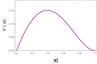
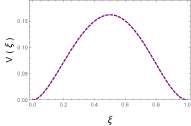
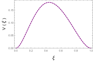
Figure 1: First row: Potential for the axial modes in GR. Second row: The potential for the axial modes ($V^{(-)}$, left panel) and the polar modes ($V^{(+)}$, right panel).

6.3 Spectrum of the Regge-Wheeler equation: axial modes

Using the AIM, we obtained the spectrum for 198 (red dots) and 200 iterations (blue dots), plotted in Fig. 2, which compares GR (upper row) with pc-GR (lower row). While convergence is observed for the low damping modes ($\mid\widetilde{\omega}_{I}\mid$ small), there is still no convergence obtained for the high damping modes. In Figure 3 the axial modes are depicted for 400 iterations. Above, the GR (left panel) is compared to pc-GR (right panel) for a large range of $-\widetilde{\omega}_{I}$. In the lower row the same is plotted but for a restricted range of $-\widetilde{\omega}_{I}$. The left panel (GR) reproduces the Figure 2 in kokkotash and of Figure 5 in konoplya2011 , where also distinct methods to resolve the differential equation are resumed.

Comparing GR with pc-GR, the structure shares still some common features, namely that the figure reminds at a fish with its head to the right and its tail to the left. However, the head is moving further to the left when the number of iterations is increased, thus, it is not a physical property and has to be rejected. The left panel in Fig. 3 shows the result for GR and the right one for pc-GR. Very interesting is, that the structure of a raising branch for pc-GR from low to large damping modes is also stable. This branch can be approximated by continuum and represents a definite feature of pc-GR, which is not present in GR.

At low damping, convergence is obtained and the frequencies in pc-GR are comparable in size to GR. This changes for the large damping modes, where the frequencies are significantly larger in pc-GR than in GR.

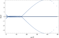
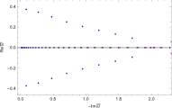
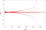
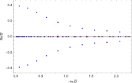
Figure 2: Spectrum of the axial modes for 200 iterations. The horizontal axis corresponds to minus the imaginary part of the frequency, which has to be positive in order to represent a damped, stable oscillation. No negative values are present, rendering the system stable. The vertical axis depicts the real part of the frequency. The first row shows the axial modes in GR, while the second row depicts the frequencies in pc-GR. The left panel shows the frequency distribution for a larger range of $-\widetilde{\omega}_{I}$ while the right panel is restricted to small damping modes.

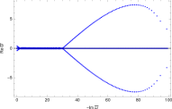
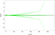
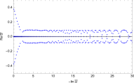
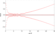
Figure 3: Spectrum of the axial modes for 400 iterations. The horizontal axis corresponds to minus the imaginary part of the frequency and the vertical axis to the real part of the complex frequency. In each row, the left panel is for GR and the right one for pc-GR. Note, that compared to 200 iterations, the onset of the ”head” is shifted far to the right in $-\widetilde{\omega}_{I}$, showing that this part is of no physical significance. For more details, in the lower row a zoom to a restricted range is shown.

6.4 Spectrum of the Zerilli equation: polar modes

In Figure 4 the polar frequency modes in pc-GR are depicted. The structure is similar to the one for the axial modes (see (3)), as expected when comparing the two potentials. In Figure 4 the red dots correspond to 200 iterations, the green dots to 300 and the blue dots to 400 iterations. Note, that convergence is clearly obtained for low values of $-\widetilde{\omega}_{I}$ and up to 30 the convergence is also acceptable. Thus the feature of a raising curve for large damping is confirmed. The ”fish head”, however, has moved further to the right, showing its unphysical nature.

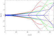
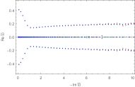
Figure 4: Spectrum of the polar modes for 200 (red dots), 300 (green dots) and 400 (blue dots) iterations. The horizontal axis corresponds to minus the imaginary part of the frequency, which has to be positive for a damped oscillation. No negative values are present, rendering the system stable. The vertical axis depicts the real part of the frequency. The left panel shows the frequency distribution for a larger range of $-\widetilde{\omega}_{I}$ while the right panel is restricted to small damping modes. Note, how the ”fish-head” moves further to the right when the iteration number is increased.

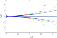
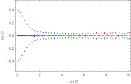
Figure 5: Comparison of axial to polar modes in pc-GR (left and right panel, respectively), depicting 300 (red dots), 400 (green dots) and 500 (blue dots) iterations. The upper row shows a large range in $-\widetilde{\omega}_{I}$ and the lower row is a zoom to the lowest region. Note the structural similarity of the axial to polar modes, suggesting an equivalence, though not perfect, as in GR.

In Fig. 5 a comparison of axial to polar modes within pc-GR is shown. In the upper row, with a wide range of $-\widetilde{\omega}_{I}$, the structure seems to be similar up to large values of $-\widetilde{\omega}_{I}$. In the lower row a Zoom to small values of $-\widetilde{\omega}_{I}$ is depicted. The $\widetilde{\omega}_{R}$ polar modes are in general larger in pc-GR than in GR.

That there is a branch in the frequency spectrum which has larger frequencies $\widetilde{\omega}_{R}$ in pc-GR than in GR is of importance: The real part of the frequency is given by $\widetilde{\omega}_{R}$ = $m_{0}\omega_{R}$. Using the frequency $\nu=250$Hz and transforming it to units in km^-1, one obtains an $\omega_{R}=5.24~{}10^{-3}$km^-1. In the first gravitational event observed a mass of the united system of about $m_{0}=60$ solar masses was reported. This gives a value of $\widetilde{\omega}_{R}=0.47$. This is the kind of order we also obtain. However, he mass $m_{0}$ was obtained recurring to the GR, i.e., it is theory based. When in a distinct theory a larger real frequency $\widetilde{\omega}_{R}$ is obtained, keeping $\omega_{R}$ the same, a larger mass is deduced. This also implies a larger release in energy and a larger deduced luminous distance, as suggested in hess-2016 .

Where the observed distribution of frequencies lies, is a matter of the dynamics of a black hole merger. A usual assumption is that all modes can in principle be excited, but only the low damping modes survive. In this scenario, no difference between axial and polar modes are expected and the results will be very similar to GR, However, when the dynamics permits to excite principally large damping modes, there might be some hope to distinguish the theories and clarification can come from explicit numerical studies. In case, large damping modes are excited only, one way to detect a difference is to search, for case of large damping modes, for simultaneous light events in the same region of the sky where the merger is observed. If consistently this light event is at larger distances than the deduced event, using GR, then it will be in favor of the existence of additional terms in the metric. This depends also on the requirement that a light event is produced, requiring some mass distribution near to the event, as an accretions disc.

7 Conclusions

Axial and polar modes where calculated over a wide range of damping, within the General Relativity (GR) and possible extensions, involving a parametric mass-function $m(r)$, whose leading term correction is proportional to $1/r^{4}$. In particular the pseudo-complex General Relativity (pc-GR), leads to such a particular extension of the parameter mass-function. This mass-function includes a coupling constant of the central mass to the dark energy and it was chosen such that still an event-horizon exists, resulting in an easier treatment of the QNM, analog to the one in standard GR. The Regge-Wheeler equation for the axial modes and the Zerilli equation for the polar modes were derived, with their corresponding potentials. After having constructed $\gamma(r)$, it was shown that axial and polar modes, though different, still share some common features. Isospectrality is not maintained, a feature we still would like to understand and we refer to future work in progress. The modes were found to be stable, implying that the corrections to the metric lead to consistent results.

Adding a further $r$-dependence to the mass-function leads to a branch of frequencies at high damping, resulting in larger deduced masses than in GR, while for low damping no large differences are observed.

Assuming that all frequencies are excited, only the low damping modes survive, resulting in no detectable differences between pcGR and GR. However, when the frequencies distribution in a merger lies in the large damping region, the deduced masses in the extended version are larger, implying also a larger distance to a gravitational wave event. If one detects at the same time of this event a light emission, the two observations result in a different distance using GR.

The present results serve as a starting point to understand the changes involved in the frequency distribution of the ring down modes in extending the theory of GR, which results in a parametric mass-function $m(r)$ in the metric components.

In the Appendices explicit derivation of the ansatz for $Z^{(+)}$ is given, which includes the one proposed by S. Chandrasekhar in chandra ; chandra1975a .

In a future publication, we will address the pc-Kerr metric, with however more involved equations. This will pose a problem to the numerical method used.

Appendix A: Axial potential

Using $Q=rZ^{(-)}$ gives for the first term in (24)

$$\Delta\frac{d}{dr}\frac{\Delta}{r^{4}}\frac{dQ}{dr}~{}=~{}\Delta\frac{d}{dr}\frac{\Delta}{r^{4}}\left[r\frac{d}{dr}Z^{(-)}+Z^{(-)}\right]$$

$$~{}=~{}\Delta\frac{d}{dr}\left[\frac{\Delta}{r^{3}}\frac{dZ^{(-)}}{dr}+\frac{\Delta}{r^{4}}Z^{(-)}\right]$$

$$~{}=~{}\Delta\left[\frac{d}{dr}\left(\frac{\Delta}{r^{4}}\right)Z^{(-)}+\frac{\Delta}{r^{4}}\frac{dZ^{(-)}}{dr}\right]+\Delta\left[\frac{1}{r}\frac{\Delta}{r^{2}}\frac{dZ^{(-1)}}{dr}\right]$$

$$~{}=~{}\Delta\left[\frac{d}{dr}\left(\frac{\Delta}{r^{4}}\right)Z^{(-)}+\frac{\Delta}{r^{4}}\frac{dZ^{(-)}}{dr}\right]-\left(\frac{\Delta}{r^{2}}\right)^{2}\frac{dZ^{(-)}}{dr}+\frac{\Delta}{r}\frac{d}{dr}\frac{\Delta}{r^{2}}\frac{dZ^{(-)}}{dr}~{}~{}~{}.$$ (71)

Using that $\frac{\Delta}{r^{2}}\frac{d}{dr}=\frac{d}{dr_{*}}$, we arrive finally at

$$r\frac{d^{2}Z^{(-)}}{dr_{*}^{2}}+\Delta\frac{d}{dr}\left(\frac{\Delta}{r^{4}}\right)Z^{(-)}~{}~{}~{}.$$ (72)

This has to be substituted into the differential equation (24), leading to

$$r\frac{d^{2}}{dr_{*}^{2}}Z^{(-)}+\Delta\frac{d}{dr}\left(\frac{\Delta}{r^{4}}\right)Z^{(-)}-\mu^{2}\frac{\Delta}{r^{3}}Z^{(-)}+r\omega^{2}Z^{(-)} = 0~{}~{}~{}.$$ (73)

Dividing by $r$ and reordering the terms in this differential equation, leads to (27), with the potential given in (29).

Appendix B: Ansatz for the polar mode wave function

The MATHEMATICA code, used to derive the equations in this section, can be retrieved from matdetails .

The general ansatz (36) is used, also valid for a constant mass-function, for which the expression in chandra ; chandra1975b is recovered.

Using (36), namely

$$Z^{(+)}(r) = \alpha(r)N(r)+\beta(r)V(r)+\gamma(r)LX(r)$$ (74)

and applying the operator $\frac{d^{2}}{dr_{*}^{2}}$ to $Z^{(+)}(r)$, we found matdetails that the factor of $N(r)$ does not depend on the frequency squared $\omega^{2}$, only the factors of $V(r)$ and $LX(r)$ do. We use the definitions

$$LX(r) = L(r)+X(r)$$

$$X(r) = nV(r)~{}~{}~{}.$$ (75)

Concentrating only on the component proportional to $\omega^{2}$, one should obtain for the factor of $V(r)$ and $LX(r)$ the result $-\omega^{2}$ $\left(\beta(r)V(r)+\gamma(r)LX(r)\right)$. The factor obtained after the application of $\frac{d^{2}}{dr_{*}^{2}}$ onto $V(r)$ is $\left(n\alpha(r)-\beta(r)\right)$, which must be equated to $-\beta(r)$. This demands

$$\alpha(r)=0~{}~{}~{}.$$ (76)

This automatically reduces (74) to $Z^{(+)}(r)=\beta(r)V(r)+\gamma(r)LX(r)$.

For the factor of $LX(r)$, restricting to the one proportional to $\omega^{2}$, and using (76) we obtain $-2\beta(r)+n\gamma(r)+2r\beta^{\prime}(r)$ = $n\gamma(r)$ (the prime refers to the derivative in $r$), which leads to the differential equation

$$\beta^{\prime} = \frac{1}{r}\beta~{}~{}~{},$$ (77)

with the solution

$$\beta(r) = r~{}~{}~{}.$$ (78)

The $\gamma(r)$ function was determined earlier and is given in (39) As seen in Appendix C, this solution satisfies the equation $G(r)=0$ (40) in a wide range of $r$, save near the point $r=\frac{3}{2}m_{0}$, implying that the Zerilli equation can be approximately constructed, with a quite small error.

Appendix C: Comparison of $V^{(+)}_{V}$ with $V^{(+)}_{LX}$, using (39) for $\gamma(r)$

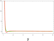
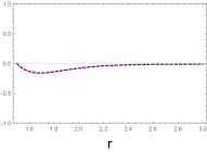
Figure 6: The left hand side depicts the two functions $V(r)$ (green online) and $VLX(r)$ (red online) in a wide range of $r$. The right panel shows the difference $\left(V(r)-VLX(r)\right)$ in a limited region in r.

In this appendix we analyze the functions $V^{(+)}(r)$, $V^{(+)}(r)$ and their difference, which is proportional to the condition (40).

On the left panel of Fig. 6 the two potentials $V_{V}^{(+)}$ and $V_{LX}^{(+)}$ are compared for a wide range of $r$. The potentials were extended to $r<\frac{3}{2}$ in order to appreciate the agreement of both potentials, using the $\gamma(r)$ as given in (39). The two functions agree very well in a wide range of $r$. The only difference appears near $r=\frac{3}{2}$, which is shown in a reduced scale on the right hand side of the figure, where, the difference $G(r)$ = $\left(V_{V}^{(+)}-V_{LX}^{(+)}\right)$ is depicted. All in all, the expression for $\gamma(r)$ works very well, however with the grain of salt that the Zerilli equation is not identically satisfied.

References

- (1) C. M. Will, The confrontation between general relativity and experiment, Living Rev. Relativ. 9, 3 (2006).
- (2) M. Maggiore, Gravitational Waves , Oxford University Press, Oxford, (2008).
- (3) Abbott B. P. et al. (LIGO Scientific Collaboration and Virgo Collaboration), Observation of Gravitational Waves from a Binary Black Hole Merger, Phys. Rev. Lett. 116, 061102 (2016).
- (4) Abbott B. P. et al. (LIGO Scientific Collaboration and The Virgo Collaboration), GW151226: Observation of Gravitational Waves from a 22-Solar-Mass Binary Black Hole Coalescence, Phys. Rev. Lett. 116, 241103 (2016).
- (5) R. A. Hulse, J. H. Taylor, A high sensitivity pulsar survey, ApJ 191, L59 (1974).
- (6) R. Adler, M. Bazin and M. Schiffer, Introduction to General Relativity, McGraw-Hill, New York, (1975).
- (7) C. W. Misner, K. S, Thorne and J. A. Wheeler. Gravitation, H. W. Freeman and Company, San Francisco, (1973).
- (8) P. O. Hess, The black hole merger event GW150914 within a modified theory of general relativity, MNRAS 462, 3026 (2016).
- (9) L. Rezzolla and O. Zanotti, Relativistic Hydrodynamics, Oxford University Press, Oxford, UK, (2013)
- (10) S. Chandrasekhar, The mathematical Theory of Black Holes, International Series of Monographs on Physics 69, Clarendon Press, Oxford, (1983).
- (11) S. Chandraskhar, On the Equations Governing the Perturbations of the Schwarzschild Black Hole, Proc. Roy. Soc. London, Series A, Math. and Phys. Sciences 343, 289 (1975).
- (12) S. Chandrasekhar and S. Detweiler, The Quasi-Normal Modes of the Schwarzschild Black Hole, Proc. Roy. Soc. London, Series A, Math. and Phys. Sciences 344, 441 (1975).
- (13) F. J. Zerilli, Effective potential for even-parity Regge-Wheeler gravitational perturbation equations, Phys. Rev. Lett. 24, 737 (1970).
- (14) T. Regge and J. A. Wheeler, Stability of a Schwarzschild singularity, Phys. Rev. 108, 1063 (1957).
- (15) H. Ciftci, R. L. Hall and N. Saad, N., Asymptotic iteration method for eigenvalue problems, J. Phys. A 36, 11807 (2003).
- (16) H. Ciftci, R. L. Hall and N. Saad, Perturbation theory from an iteration method, Phys. Lett. A 340, 388 (2005).
- (17) H. Cho, A. S. Cornell, J. Doukas, T.-R. Huang and W. Naylor, A New Approach to Black Hole Quasinormal Modes: A Review of the Asymptotic Iteration Method, Adv. in Math. Phys. 2012, 281705 (2012).
- (18) P. O.Hess, W. Greiner, Pseudo-complex General Relativity, Int. J. Mod. Phys. E 18, 51 (2009).
- (19) Hess P. O., Schäfer M., Greiner W., Pseudo-Complex General Relativity, Springer, Heidelberg, Germany, (2015).
- (20) T. Schönenbach, G. Caspar, P.O. Hess, T. Boller, A. Müller, W. Greiner, MNRAS 430, 2999 (2013)
- (21) T. Schönenbach, G. Caspar, P.O. Hess, T. Boller, A. Müller, W. Greiner, MNRAS 442, 121–130 (2014).
- (22) P. O. Hess, Adv. in High Energy Phys., Review on the pseudo-complex General Relativity and dark energy, 2019, 1840360 (2019).
- (23) P. O. Hess, E. López-Moreno, Kerr Black Holes within a Modified Theory of Gravity, Universe 5, 191 (2019).
- (24) P. O. Hess, Progr. Part. and Nucl. Phys., Alternatives to Einstein’s General Relativity Theory, 114, 103809 (2020).
- (25) MATHEMATICA 11.3.0.0; Wolfram Research Foundation: Champaign, IL, USA, 2018.
- (26) https://github.com/peterottohess/gravitationalwavesSchwarzschild/
- (27) K. D. Kokkotash and B. G. Schmidt, Quasi-normal modes of stars and black holes, Living Reviews in Relativity 2, article no. 2 (1999).
- (28) R. A. Konoplya and A. Zhidenko, Quasinormal modes of black holes: From astrophysics to string theory, Rev. Mod. Phys. 83, 793 (2011).
- (29) A. Nielsen, O. Birnholz, Testing pseudo-complex General Relativity with gravitational waves, AN 339, 298 (2018).
- (30) A. Nielsen, O. Birnholz, Gravitational wave bounds on dirty black holes, AN 340, 116 (2019).
- (31) F. Cooper, A. Khare and U. Sukhatme, Supersymmetry and Quantum Mechanics, Phys. Rep. 251, 267 (1995).
- (32) F. Moulin and A. Barrau, Analytical proof of the isospectrality of quasimnormal modes for Schwarzschild-de Sitter-Anti-de Sitter specetimes, Gen. Rel. and Grav. 52, 82 (2020).