Evolution of a Non-Hermitian Quantum Single-Molecule Junction at Constant Temperature

Abstract

This work concerns the theoretical description of the quantum dynamics of molecular junctions with thermal fluctuations and probability losses To this end, we propose a theory for describing non-Hermitian quantum systems embedded in constant-temperature environments. Along the lines discussed in [A. Sergi et al, Symmetry 10 518 (2018)], we adopt the operator-valued Wigner formulation of quantum mechanics (wherein the density matrix depends on the points of the Wigner phase space associated to the system) and derive a non-linear equation of motion. Moreover, we introduce a model for a non-Hermitian quantum single-molecule junction (nHQSMJ). In this model the leads are mapped to a tunneling two-level system, which is in turn coupled to a harmonic mode (i.e., the molecule). A decay operator acting on the two-level system describes phenomenologically probability losses. Finally, the temperature of the molecule is controlled by means of a Nosé-Hoover chain thermostat. A numerical study of the quantum dynamics of this toy model at different temperatures is reported. We find that the combined action of probability losses and thermal fluctuations assists quantum transport through the molecular junction. The possibility that the formalism here presented can be extended to treat both more quantum states ($\sim 10$) and many more classical modes or atomic particles ($\sim 10^{3}-10^{5}$) is highlighted.

Keywords: molecular junction; non-Hermitian quantum mechanics; open quantum system dynamics; quantum thermodynamics

PACS: 31.15.xg; 02.60.Cb, 05.30.-d; 05.60.Gg, 03.67.Pp

MSC: 80M99; 81-08; 81-10, 81P99

I Introduction

Molecular junctions are nano-devices composed of metal or semiconductor electrodes known as leads hystory ; thoss . A single molecule simulates a conducting bridge between the leads. Such a nanostructure is almost perfectly suited to study non-equilibrium quantum transport hystory ; thoss .

Various approaches satisfactorily befit the investigation of the phenomenology of molecular junctions thoss . In this work, we introduce a simple toy model of a molecular junction thoss in order to perform a qualitative study aimed at singling out universal features of such systems. To this end, the operator-valued Wigner formulation of quantum mechanics quasi_lie ; zhang-balescu ; balescu-zhang is particularly useful to embed quantum toy-models in quantum phase space baths since it can simultaneously describe dissipative phenomena and thermal fluctuations. A quantum-classical molecular junction model has been studied in Ref. hanna2 .

In general, theories of quantum transport offer an acceptable representation of excitations and state population transfer. They usually assume that what is transferred does not disintegrate or disappear from the system. Such a physical property is expressed through the conservation of probability. On the contrary, by definition, the probability in quantum systems with gain and loss is not conserved. Such a feature can be incorporated in the theory by introducing non-Hermitian Hamiltonians gamow_1928 ; carlbenderpt ; mostafazadeh_2002 ; subotnik ; zelovich ; zelovich2 . Recently, the development of non-Hermitian quantum mechanics (NHQM) has been propelled by various experiments on many systems (see rotter_15 ; moiseyev_11 and references therein). While in this work a non-equilibrium quantum statistical mechanics of molecular junctions is adopted, linear equations of motion are used in Refs. subotnik ; zelovich ; zelovich2 . Conceptually, this can be understood in terms of the different theoretical targets: In Refs. subotnik ; zelovich ; zelovich2 the target is to study non-equilibrium transport per se. Instead, our work is aimed at showing the possibility of a statistical mechanical description for non-Hermitian quantum systems in classical bath as_15 .

Since probability non-conserving quantum systems are open quantum systems rotter_15 , it is natural to formulate NHQM in terms of the density matrix as_15 ; sz_13 ; sz_15 ; sz_16 ; entropy2 ; grima_18 ; nh_emwave ; sust . Typically, a non-Hermitian Hamiltonian is either derived by means of the Feshbach formalism f-58 ; f-62 or it is postulated as an ansatz (see Refs. sz_13 ; as_15 ; sz_15 ; sz_16 ; entropy2 ; grima_18 ; nh_emwave ; sust ). It is remarkable that there is a third possibility according to which a non-Hermitian Hamiltonian may arise from stroboscopic measurements performed on an ancilla-subsystem added to a quantum system, a very interesting process capable of generating entanglement noi . Given a non-Hermitian Hamiltonian and assuming that the Schrödinger equation is still valid, one derives a probability non-conserving equation of motion for the density matrix of the system noi . However, in order to meet the need of establishing a proper quantum statistical theory, this non-Hermitian equation of motion for the density matrix is generalized into a non linear-one as_15 ; sz_13 ; sz_15 ; sz_16 ; entropy2 ; grima_18 ; nh_emwave ; sust . Essentially, this is the origin of the difference between the linear approach of subotnik ; zelovich ; zelovich2 and the non-linear approach of as_15 ; sz_13 ; sz_15 ; sz_16 ; entropy2 ; grima_18 ; nh_emwave ; sust .

Various investigations on thermal effects in molecular junctions are found in the literature jtherm3 ; jtherm4 ; jtherm5 . However, to the best of our knowledge, thermal effects have been investigated separately from probability losses of molecular junctions. In light of the previous considerations, the purpose of this work is to combine the non-linear equation for the density matrix of a system with a non-Hermitian Hamiltonian and temperature control in quantum phase space dynamics ap . Temperature control is technically implemented by means of the Nosé-Hoover chain nhc thermostat, formulated in terms of quasi-Lie brackets quasi_lie . The unified formalism here reported is developed for studying a greater variety of phenomena than those accessible to theories treating thermal fluctuations and probability losses separately. In detail, the theory is obtained through the density matrix approach to non-Hermitian quantum mechanics as_15 ; sz_13 ; sz_15 ; sz_16 ; entropy2 ; grima_18 ; nh_emwave ; sust and it is expressed in terms of the operator-valued formulation of quantum mechanics quasi_lie ; zhang-balescu ; balescu-zhang ; as_15 . For clarity, we highlight the three mathematical ingredients that must be combined for building our formulation. First, we need an approach for describing quantum operators in terms of operator-valued Wigner phase space functions. The conceptual framework of this specific theory assumes an Eulerian picture where a Hilbert space, or a space of quantum discrete states, is defined for each point $X=(Q,P)$ of phase space. Accordingly, the operator-valued Wigner function quasi_lie ; zhang-balescu ; balescu-zhang may also be called phase-space-dependent density matrix. The consistent coupling of quantum and phase space degrees of freedom requires that quantum dynamics in the Hilbert space associated to $X$ also depends non-locally on the quantum dynamics associated to different points $X^{\prime}$. Likewise, the dynamics of $X$ does not only depend on its quantum space but it also depends on the quantum spaces of other points $X^{\prime}$ and viceversa. In practice, such a dependence can be implemented through a variety of algorithms theochem ; sstp ; algo12 ; algo15 . When the Hamiltonian is quadratic, one can expand the operator-valued Moyal bracket b3 ; b4 up to linear order in $\hbar$ and obtain quantum equations of motion mackernan .

The second ingredient entering our theory is the requirement that the degrees of freedom in phase space evolve in time satisfying the constraint determined by the constant thermodynamic temperature. The temperature control of the classical degrees of freedom is achieved in silico by means of the Nosé-Hoover chain algorithm nhc . We find such an approach advantageous because the formulation of the Nosé-Hoover chain algorithm can be realized within the theoretical framework given by the quasi-Lie brackets quasi_lie . Such brackets allow one to generalize the Nosé-Hoover chain algorithm, originally formulated for classical systems only, to the more general case of the operator-valued formulation of quantum mechanics ap ; b3 ; b4 .

The third ingredient, of course, is that the modeling of the leads provides a non-Hermitian quantum system per se.

When all these three theoretical features are simultaneously taken into account, we obtain an equation that generalizes the one arising from the quantum-classical quasi-Lie bracket quasi_lie because it can describe probability gain/loss as_15 too. Moreover, since such an equation keeps the thermodynamic temperature of the phase space degrees of freedom constant by means of the Nosé-Hoover chain algorithm quasi_lie ; nhc ; b3 ; b4 , it generalizes the equations used in Refs. as_15 ; sz_13 ; sz_15 ; sz_16 ; entropy2 ; grima_18 ; nh_emwave ; sust , which did not implement any thermodynamic constraint.

In this paper we investigate the time evolution of a single-molecule junction toy-model represented by a non-Hermitian Hamiltonian with a parametric phase space dependence. The isolated leads are represented by a two-level system. In this situation, the transport of the occupation probability of one or the other state can only occur through quantum tunneling. The molecule connecting the two leads is modeled by a harmonic oscillator. When we consider only the coupling between the harmonic mode and the two-level system, the total system is considered closed. In this case, transport can take place both via tunneling and via the channel given by the oscillator. In order to build a complete non-Hermitian quantum single-molecule junction model at constant temperature, the closed spin-boson system is transformed into an open quantum system by means of two theoretical steps. The first step is to consider a decay operator acting on the two-level system. This operator introduces another transport channel that does not conserve probability and then breaks time-reversibility.

The second step is to put the harmonic mode into contact with a heat bath. Of course, this condition forces the molecule to have the same temperature of the bath and to experience fluctuations according to the canonical ensemble probability distribution. In practice, the action of the constant-temperature bath on the molecule is implemented by means of the Nosé-Hoover chain thermostat. For this reason, in the following we will use wording such as “heat bath”, “constant-temperature environment” or “Nosé-Hoover chain thermostat” interchangeably.

The final complete non-Hermitian Hamiltonian is designed to represent two lossy leads interacting with a thermalized molecule.

The organization of the paper is the following: In Sec. II we give a short summary of the density matrix approach to the dynamics of a system governed by a non-Hermitian Hamiltonian. In Sec. III we describe briefly how to treat non-Hermitian quantum systems interacting with classical degrees of freedom. We present the main theoretical results of this work in Sec. IV, where we introduce the mathematical formalism describing the quantum dynamics of a non-Hermitian quantum system interacting with classical degrees of freedom at constant temperature. In Sec. V we introduce the non-Hermitian quantum single-molecule junction model. The results of the numerical calculations are reported in Sec. VI. Finally, our conclusions are given in Sec. VII.

II Quantum dynamics of non-Hermitian systems

Consider a quantum system described by a non-Hermitian Hamiltonian operator

$$\hat{\cal H}=\hat{H}-i\hat{\Gamma}\;,$$ (1)

where $\hat{H}$ and $\hat{\Gamma}$ are Hermitian operators ($\hat{\Gamma}$ is the decay operator). In the presence of a probability sink or source, the dynamics of the system is defined in terms of the following equations (we set $\hbar=1$):

$$\frac{d}{dt}|\Psi(t)\rangle = -i\hat{\cal H}|\Psi(t)\rangle\;,$$ (2)

$$\frac{d}{dt}\langle\Psi(t)| = i\langle\Psi(t)|\hat{\cal H}^{\dagger}\;,$$ (3)

where $|\Psi(t)\rangle$ and $\langle\Psi(t)|$ are state vectors of the system. Equations (2) and (3) reduce to the standard Schrödinger equation when $\hat{\Gamma}=0$.

The density matrix approach to non-Hermitian quantum systems as_15 ; sz_13 ; sz_15 ; sz_16 ; entropy2 ; grima_18 ; nh_emwave ; sust is obtained upon introducing at any t>0 a Hermitian, semipositive defined, but non-normalized density matrix

$$\hat{\Omega}(t)=|\Psi(t)\rangle\langle\Psi(t)|\;.$$ (4)

The equation of motion for $\hat{\Omega}$ sz_13 ; grima_18 ; sust is obtained by taking the time derivative of Eq. (4) and using Eq. (1):

$$\frac{d}{dt}\hat{\Omega}(t)=-i\left[\hat{H},\hat{\Omega}(t)\right]-\left[\hat{\Gamma},\hat{\Omega}(t)\right]_{+}\;,$$ (5)

where $[...,...]$ is the commutator and $[...,...]_{+}$ is the anticommutator. Equation (5) is linear but, nevertheless, it describes an open quantum system. This is possible since it is defined in terms of a decay operator that physically describes the presence of probability sources/sinks, arising from the hidden system with which the open quantum system interacts.

Equation (5) is non-Hermitian, breaks time reversibility and does not conserve the trace of $\hat{\Omega}(t)$. In fact, from Eq. (5) one can easily derive

$$\frac{d}{dt}{\rm Tr}\left(\hat{\Omega}(t)\right)=-2{\rm Tr}\left(\hat{\Gamma}\hat{\Omega}(t)\right)\;.$$ (6)

In order to obtain a well-founded statistical mechanics of non-Hermitian quantum systems, one can introduce the normalized density matrix

$$\hat{\rho}(t)=\frac{\hat{\Omega}(t)}{{\rm Tr}\left(\hat{\Omega}(t)\right)}\;.$$ (7)

This operator $\hat{\rho}(t)$ obeys the non-linear equation

$$\frac{d}{dt}\hat{\rho}(t)=-i\left[\hat{H},\hat{\rho}(t)\right]-\left[\hat{\Gamma},\hat{\rho}(t)\right]_{+}+2\hat{\rho}(t){\rm Tr}\left(\hat{\Gamma}\hat{\rho}(t)\right)\;.$$ (8)

As a consequence of its very definition and of Eq. (8), ${\rm Tr}(\hat{\rho}(t))=1$ at all times. Equation (8) breaks time reversal symmetry and is non-linear. In practice, the formalism trades off the non-conservation of probability in Eq. (5) with the non-linearity of Eq. (8). As the linear Eq. (5), the non-linear Eq. (8) describes the dynamics of an open quantum system. Consistently, averages of arbitrary operators, e.g., $\hat{\chi}$, can be calculated by means of the normalized density matrix $\hat{\rho}$ as

$$\langle\hat{\chi}\rangle_{(t)}={\rm Tr}\left(\hat{\rho}(t)\hat{\chi}\right)\;.$$ (9)

Equation (9) establishes the foundations of the statistical interpretation of non-Hermitian quantum mechanics.

III Non-Hermitian quantum systems set in phase space

Non-Hermitian quantum systems can be embedded in phase space as_15 . In the following, we sketch the derivation given in as_15 . Let us consider a system described by a hybrid set of coordinates $(\hat{x},X)$, where $\hat{x}$ are quantum coordinates (operators) and $X=(Q,P)$ are phase space coordinates (an obvious multidimensional notation is used in order not to clutter formulas with too many indices). In this specific case, the $X$s describe the phase space coordinates of the system. As we have already discussed in the Introduction, the description of the system, using the operator-valued-formulation of quantum mechanics, can be established via an Eulerian point of view according to which a space of state vectors is defined for any point $X$ of phase space, zhang-balescu ; balescu-zhang ; quasi_lie so that $\hat{x}$ (and operators defined in terms of $\hat{x}$) can act on it. In such a hybrid space there are operators that depend only on $\hat{x}$, which we denote with the symbol $\hat{\phantom{x}}$ on top of the operator, e.g., $\hat{\Gamma}$. There are pure phase space functions which we denote by their arguments, e.g., $H_{\rm B}(X)$, or $G(X,t)$ when there is also an explicit time dependence. Finally, there are operators that depend both on $\hat{x}$ and (parametrically) on $X$. We denote the latters with the symbol $\tilde{\phantom{x}}$ on top, e.g., $\tilde{\Omega}(t)\equiv\hat{\Omega}(X,t)$.

In the non-Hermitian case, we consider a Hamiltonian operator with parametric dependence on phase space

$$\tilde{\cal H} = \hat{H}+H_{\rm B}(X)+\tilde{H}_{I}-i\hat{\Gamma}$$ (10)

$$= \tilde{H}_{\rm S}-i\hat{\Gamma}\;,$$

where $\hat{H}$ is the Hermitian Hamiltonian of the quantum subsystem, $H_{\rm B}(X)$ is the Hamiltonian of the degrees of freedom in phase space, $\tilde{H}_{I}$ describes the interaction between the quantum system and the bath, and $\tilde{H}_{\rm S}=\hat{H}+H_{\rm B}(X)+\tilde{H}_{I}$. Of course, $\tilde{\cal H}$ is the total non-Hermitian Hamiltonian of the system with $\hat{\Gamma}$ as the decay operator.

When the operator $\hat{\Gamma}$ acts on the quantum dynamical variables of the non-Hermitian quantum system, it has been shown as_15 that, as a generalization of the equations given in Refs. zhang-balescu ; balescu-zhang ; quasi_lie , the equation of motion becomes

$$\frac{\partial}{\partial t}\tilde{\Omega}(t)=-i\left[\tilde{H}_{\rm S},\tilde{\Omega}(t)\right]-\left[\hat{\Gamma},\tilde{\Omega}(t)\right]_{+}+\frac{1}{2}\left\{\tilde{H}_{\rm S},\tilde{\Omega}(t)\right\}_{\mbox{\boldmath$\cal B$}}-\frac{1}{2}\left\{\tilde{\Omega}(t),\tilde{H}_{\rm S}\right\}_{\mbox{\boldmath$\cal B$}}\;,$$ (11)

where $\tilde{\Omega}(t)$ is the phase-space-dependent non-normalized density matrix of the system and

$$\mbox{\boldmath$\cal B$}=\left[\begin{array}[]{cc}{\bf 0}&{\bf 1}\\ -{\bf 1}&{\bf 0}\end{array}\right]$$ (12)

is the symplectic matrix written in block form. Using it, one can write the Poisson bracket in the form adopted in Eq. (18):

$$\left\{\tilde{H}_{\rm S},\tilde{\Omega}(t)\right\}_{\mbox{\boldmath$\cal B$}}\equiv\sum_{I,J=1}^{2N}\frac{\partial\tilde{H}_{\rm S}}{\partial X_{I}}{\cal B}_{IJ}\frac{\partial\tilde{\Omega}(t)}{\partial X_{J}}\;.$$ (13)

The dimension of phase space is $2N$.

The trace of the phase-space-dependent density matrix $\tilde{\rm T}{\rm r}$ is defined as

$$\tilde{\rm T}{\rm r}\left(\tilde{\Omega}(t)\right)={\rm Tr}^{\prime}\int dX\tilde{\Omega}(X,t)\;,$$ (14)

where ${\rm Tr}^{\prime}$ denotes a partial trace over the quantum dynamical variables $\hat{x}$ and $\int dX$ is the integral in phase space. The trace $\tilde{\rm T}{\rm r}\left(\tilde{\Omega}(t)\right)$ obeys the equation of motion

$$\frac{d}{dt}\tilde{\rm T}{\rm r}\left(\tilde{\Omega}(t)\right)=-2\tilde{\rm T}{\rm r}\left(\hat{\Gamma}\tilde{\Omega}(t)\right)\;.$$ (15)

The result given in Eq. (15) is proven in Appendix A.

Let us now introduce a phase-space-dependent normalized density matrix $\tilde{\rho}(X,t)$:

$$\tilde{\rho}(X,t)=\frac{\tilde{\Omega}(X,t)}{\tilde{\rm T}{\rm r}\left(\tilde{\Omega}(X,t)\right)}\;.$$ (16)

Quantum statistical averages of an arbitrary phase-space-dependent operator $\tilde{\chi}$ can now be calculated as

$$\langle\tilde{\chi}\rangle_{(t)}=\tilde{\rm T}{\rm r}\left(\tilde{\rho}(t)\tilde{\chi}\right)\;.$$ (17)

The phase-space-dependent normalized density matrix obeys the non-linear equation of motion below

$$\frac{\partial}{\partial t}\tilde{\rho}(t)=-i\left[\tilde{H}_{\rm S},\tilde{\rho}(t)\right]-\left[\hat{\Gamma},\tilde{\rho}(t)\right]_{+}+2\hat{\rho}(t)\tilde{\rm T}{\rm r}\left(\hat{\Gamma}\tilde{\rho}(t)\right)+\frac{1}{2}\left\{\tilde{H}_{\rm S},\tilde{\rho}(t)\right\}_{\mbox{\boldmath$\cal B$}}-\frac{1}{2}\left\{\tilde{\rho}(t),\tilde{H}_{\rm S}\right\}_{\mbox{\boldmath$\cal B$}}\;.$$ (18)

IV Non-Hermitian quantum systems set in a constant-temperature phase space

Equations (11) and (18) describe the dynamics of non-Hermitian quantum systems embedded in phase space as_15 . When considering open quantum systems in more general settings, it is common to consider the effects of thermal fluctuations. Phase space coordinates undergo thermal fluctuations when their microscopic equilibrium state is described by the canonical distribution function. In this ensemble the thermodynamic temperature is constant. Within the framework of the operator-valued Wigner formulation of quantum mechanics zhang-balescu ; balescu-zhang ; quasi_lie , temperature constraints are efficiently formulated by means of quasi-Lie brackets quasi_lie ; b3 ; b4 . In the classical case, deterministic thermostats, such as the Nosé-Hoover chain thermostat nhc , are also implemented by means of quasi-Lie brackets b1 ; b2 ; aspvg . Below, we briefly explain how this is achieved. In silico (i.e., on the computer), temperature control is realized by augmenting the dimensions of phase space using just a few additional degrees of freedom. The new higher dimensional phase space is known as extended phase space. We indicate points in the extended phase space by means of the symbol $X^{\rm e}$. In the case of the Nosé-Hoover chain thermostat, upon introducing two fictitious coordinates $\Lambda_{1},\Lambda_{2}$ with their associated momenta $\Pi_{1},\Pi_{2}$, we have the following point in the extended phase space:

$$X^{\rm e}=(Q,\Lambda_{1},\Lambda_{2},P,\Pi_{1},\Pi_{2})\;.$$ (19)

To lighten the notation, the phase space coordinates of the Nosé-Hoover chain thermostat are denoted as ${\cal Y}=(\Lambda_{1},\Lambda_{2},\Pi_{1},\Pi_{2})$. For the reader, the symbol $\cal Y$ denotes a calligraphic $Y$. A generic operator acting upon the extended phase space is identifiable by the apex e. Considering a classical system with a potential term $V(Q)$ and Hamiltonian $H_{\rm B}(X)=P^{2}/2+V(Q)$, the extended phase space Hamiltonian (see b1 ; b2 ; aspvg and references therein) includes the Nosé-Hoover chain energy nhc ; b1 and is defined as

$$H^{\rm e}(X^{\rm e}) = H_{\rm B}(X)+\sum_{K=1}^{2}\left(\frac{\Pi_{K}^{2}}{2\mu_{K}}\right)+gk_{\rm B}T\Lambda_{1}+k_{\rm B}T\Lambda_{2}$$ (20)

$$= H_{\rm B}(X)+H_{nhc}({\cal Y})\;,$$

where $\mu_{K}$ are fictitious inertial parameters, $T$ is the termodynamic temperature, $k_{\rm B}$ is the Boltzmann constant, $N$ is the number of physical coordinates $Q$ that are thermalized. The equation of motion in extended phase space can be written as:

$$\dot{X}_{K}^{\rm e}=\left\{X_{K}^{\rm e},H^{\rm e}\right\}_{\mbox{\boldmath$\cal B$}^{\rm e}}=\sum_{I,J=1}^{2(N+2)}\frac{\partial X_{K}^{\rm e}}{\partial X_{I}^{\rm e}}{\cal B}_{IJ}^{\rm e}\frac{\partial H^{\rm e}}{\partial X_{J}^{\rm e}}=\sum_{J=1}^{2(N+2)}{\cal B}_{KJ}^{\rm e}\frac{\partial H^{\rm e}}{\partial X_{J}^{\rm e}}\;,$$ (21)

where the first and second equality define a quasi-Lie bracket. The last equality enlighten the matrix structure of the equations of motion. This last form also allows one to compactly define the compressibility of phase space:

$$\kappa^{\rm e}\equiv\sum_{I=1}^{2(N+2)}\frac{\partial\dot{X}_{I}^{\rm e}}{\partial X_{I}^{\rm e}}=\sum_{I,J=1}^{2(N+2)}\frac{\partial{\cal B}_{IJ}^{\rm e}}{\partial X_{I}^{\rm e}}\frac{\partial H^{\rm e}}{\partial X_{J}^{\rm e}}=-N\frac{\dot{\Pi}_{1}}{\mu_{1}}-\frac{\dot{\Pi}_{2}}{\mu_{2}}\;,$$ (22)

The antisymmetric matrix $\mbox{\boldmath$\cal B$}^{\rm e}$, entering Eqs. (21) and (22), defined as

$$\mbox{\boldmath$\cal B$}^{\rm e}=\left[\begin{array}[]{cccccc}0&0&0&1&0&0\\ 0&0&0&0&1&0\\ 0&0&0&0&0&1\\ -1&0&0&0&-P&0\\ 0&-1&0&P&0&-\Pi_{1}\\ 0&0&-1&0&\Pi_{1}&0\end{array}\right]\;,$$ (23)

is an antisymmetric phase-space-dependent matrix generalizing the symplectic matrix in Eq. (12). Equation (21) is called a quasi-Hamiltonian equation because, while conserving $H^{\rm e}(X^{\rm e})$, it cannot be derived from the Hamiltonian formalism alone: in order to write the equation of motion (21), together with $H^{\rm e}(X^{\rm e})$, one also needs the antisymmetric matrix $\mbox{\boldmath$\cal B$}^{\rm e}$ in Eq. (23). The equation of motion for the distribution function $f(X^{\rm e},t)$ is

$$\frac{\partial}{\partial t}f(t)=-\left\{f(t),H^{\rm e}\right\}_{\mbox{\boldmath$\cal B$}^{\rm e}}-\kappa^{\rm e}f(t)\;.$$ (24)

Given the discussion above, our task becomes that of generalizing Eq. (24) to a non-Hermitian quantum system. The phase-space-dependent Hamiltonian of the quantum system must be defined on the extended phase space of the Nosé-Hoover Chain thermostat:

$$\tilde{\cal H}^{\rm e} = \hat{H}+H_{\rm B}(X)+\tilde{H}_{I}+H_{\rm nhc}({\cal Y})-i\hat{\Gamma}$$ (25)

$$= \tilde{H}_{\rm S}^{\rm e}-i\hat{\Gamma}\;.$$

A phase-space-dependent non-normalized density matrix $\tilde{\Omega}^{\rm e}(t)$ can be introduced as well. We postulate that $\tilde{\Omega}^{\rm e}(t)$ obeys the equation of motion

$$\frac{\partial}{\partial t}\tilde{\Omega}^{\rm e}(t)=-i\left[\tilde{H}_{\rm S}^{\rm e},\tilde{\Omega}^{\rm e}(t)\right]-\left[\hat{\Gamma},\tilde{\Omega}^{\rm e}(t)\right]_{+}+\frac{1}{2}\left\{\tilde{H}_{\rm S}^{\rm e},\tilde{\Omega}^{\rm e}\right\}_{\mbox{\boldmath$\cal B$}^{\rm e}}-\frac{1}{2}\left\{\tilde{\Omega}^{\rm e},\tilde{H}_{\rm S}^{\rm e}\right\}_{\mbox{\boldmath$\cal B$}^{\rm e}}-\kappa_{\rm S}^{\rm e}\tilde{\Omega}^{\rm e}(t)\;.$$ (26)

In absence of quantum degrees of freedom, Eq. (26) reduces correctly to the Eq. (24). Moreover, when $(\Lambda_{I},\Pi_{I})\to 0$, with $I=1,2$, (which means that the Nosé-Hoover thermostat is not applied), Eq. (26) reduces unerringly to Eq. (11).

The trace $\tilde{\rm T}{\rm r}^{\rm e}$ of the density matrix $\tilde{\Omega}^{\rm e}(t)$ involves an integral over the extended phase space:

$$\tilde{\rm T}{\rm r}^{\rm e}\left(\tilde{\Omega}^{\rm e}(t)\right)={\rm Tr}^{\prime}\int dX^{\rm e}\tilde{\Omega}^{\rm e}(X^{\rm e},t)\;.$$ (27)

The equation of motion of the trace defined in Eq. (27) has the same structure of Eq. (15):

$$\frac{d}{dt}\tilde{\rm T}{\rm r}^{\rm e}\left(\tilde{\Omega}^{\rm e}(t)\right)=-2\tilde{\rm T}{\rm r}^{\rm e}\left(\hat{\Gamma}\tilde{\Omega}^{\rm e}(t)\right)\;.$$ (28)

In Appendix B it is shown how Eq. (28) is obtained.

The phase-space-dependent normalized density matrix in the extended phase space, $\tilde{\rho}^{\rm e}(X^{\rm e},t)$, is defined in analogy with Eq. (16) as

$$\tilde{\rho}^{\rm e}(X^{\rm e},t)=\frac{\tilde{\Omega}^{\rm e}(X^{\rm e},t)}{\tilde{\rm T}{\rm r}^{\rm e}\left(\tilde{\Omega}^{\rm e}(X^{\rm e},t)\right)}\;.$$ (29)

In analogy with Eq. (17), quantum statistical averages are calculated as

$$\langle\tilde{\chi}^{\rm e}\rangle_{(t)}^{\rm e}=\tilde{\rm T}{\rm r}^{\rm e}\left(\tilde{\rho}^{\rm e}(t)\tilde{\chi}^{\rm e}\right)\;.$$ (30)

The phase-space-dependent normalized density matrix in Eq. (29) obeys the non-linear equation of motion:

$$\frac{\partial}{\partial t}\tilde{\rho}^{\rm e}(t) = -i\left[\tilde{H}_{\rm S}^{\rm e},\tilde{\rho}^{\rm e}(t)\right]-\left[\hat{\Gamma},\tilde{\rho}^{\rm e}(t)\right]_{+}+2\tilde{\rho}^{\rm e}(t)\tilde{\rm T}{\rm r}^{\rm e}\left(\hat{\Gamma}\tilde{\rho}^{\rm e}(t)\right)$$ (31)

$$+ \frac{1}{2}\left\{\tilde{H}_{\rm S}^{\rm e},\tilde{\rho}^{\rm e}\right\}_{\mbox{\boldmath$\cal B$}^{\rm e}}-\frac{1}{2}\left\{\tilde{\rho}^{\rm e},\tilde{H}_{\rm S}^{\rm e}\right\}_{\mbox{\boldmath$\cal B$}^{\rm e}}-\kappa_{\rm S}^{\rm e}\tilde{\rho}^{\rm e}(t)\;.$$

We remark that Eqs. (26) and (31) are two important results of this work since these equations define the dynamics of a non-Hermitian quantum system embedded in a classical bath at constant temperature.

V Model of a Non-Hermitian Quantum Single-Molecule Junction at Constant Temperature

In this section we formulate a molecular junction toy-model described by a non-Hermitian Hamiltonian denoted by $\tilde{\cal H}^{\rm m}$. The various energy contributions entering the Hermitian terms in part of the Hamiltonian model are:

$$\hat{H}^{\rm m} = -\Delta\hat{\sigma}_{z}\;,$$ (32)

$$H_{\rm B}^{\rm m}(X) = \frac{P^{2}}{2}+\frac{\omega^{2}}{2}Q^{2}\;,$$ (33)

$$\tilde{H}_{\rm I}^{\rm m}(Q) = -cQ\hat{\sigma}_{x}\;,$$ (34)

$$H_{\rm nhc}^{\rm m}({\cal Y}) = \sum_{K=1}^{2}\left(\frac{\Pi_{K}^{2}}{2\mu_{K}}+k_{B}T\Lambda_{K}\right)\;.$$ (35)

The two-level system Hamiltonian $\hat{H}^{\rm m}$ describes quantum transport between the leads in terms of the variation of the population of a ground and an excited state. The extended phase space point $X^{\rm m}$ is defined as in Eq. (21) but the model considers a single $Q$ coordinate and its conjugate momentum $\Pi$. Transport in the isolated two-level system takes place through tunneling. The inclusion in the model description of the decay operator $\hat{\Gamma}^{\rm m}$ opens a channel through which the population of the states can disappear forever from the two-level system. The explicit form of $\hat{\Gamma}^{\rm m}$ will be given later on when we transform to the adiabatic basis. This subsystem is also coupled to a harmonic mode, with free Hamiltonian $H_{\rm B}^{\rm m}(Q)$, by means of an interaction Hamiltonian $\tilde{H}_{\rm I}^{\rm m}$. The harmonic mode opens another channel for the transport of the population between the leads. In addition to this, the harmonic mode is embedded in a thermal bath via the Nosé-Hoover chain thermostat with energy $H_{\rm nhc}^{\rm m}$. The complete non-Hermitian Hamiltonian model $\tilde{\cal H}^{\rm m}$ reads

$$\tilde{\cal H}^{\rm m}(X^{\rm m}) = \hat{H}^{\rm m}+H_{\rm B}^{\rm m}(X)+\tilde{H}_{\rm I}^{\rm m}(Q)+H_{\rm nhc}^{\rm m}({\cal Y})-i\hat{\Gamma}^{\rm m}$$ (36)

$$= \tilde{H}_{\rm S}^{\rm m}(X^{\rm m})-i\hat{\Gamma}^{\rm m}\;,$$

where the last equality also defines the Hermitian part of the Hamiltonian model, i.e.,

$$\tilde{H}_{\rm S}^{\rm m}(X^{\rm m})=\hat{H}^{\rm m}+H_{\rm B}^{\rm m}(X)+\tilde{H}_{\rm I}(Q)+H_{\rm nhc}^{\rm m}({\cal Y})\;.$$ (37)

To the authors’ knowledge, the Hamiltonian model in Eq. (36) provides a novel non-linear approach to the modeling of lossy molecular junctions in thermal baths. Figure 1 displays a pictorial representation of the non-Hermitian quantum single-molecule junction (nHQSMJ) model at constant temperature.

The abstract dynamics of the nHQSMJ model is obtained upon using the non-Hermitian Hamiltonian (36) in Eq. (31). The abstract equations of motion can be represented using different basis sets. The approach described in Ref. theochem is based on the representation in the adiabatic basis. We also adopt such an approach here. The adiabatic Hamiltonian is defined as

$$\tilde{h}_{\rm ad}^{\rm m}(Q)=\hat{H}^{\rm m}+H_{\rm B}^{\rm m}(X)+\tilde{H}_{\rm I}^{\rm m}(Q)-\frac{P^{2}}{2}\;,$$ (38)

and the adiabatic basis is introduced through the eigenvalue equation

$$\tilde{h}_{\rm ad}^{\rm m}(Q)|\Phi_{\alpha}(Q)\rangle=E_{\alpha}|\Phi_{\alpha}(Q)\rangle\;.$$ (39)

In practice, the adiabatic states are a kind of dressed states of the quantum system when it interacts with approximately “frozen” classical degrees of freedom. The operator $\hat{\Gamma}^{\rm m}$ is chosen in a phenomenological way. In the adiabatic basis it is taken as

$$\hat{\Gamma}^{\rm m}=\frac{\gamma}{2}\left[\begin{array}[]{cc}1&0\\ 0&0\end{array}\right]\;.$$ (40)

In this way we describe a model where the excited state is in contact with a sink while the ground state is left unperturbed.

The abstract equation of motion for the non-normalized density matrix of the model is

$$\frac{\partial}{\partial t}\tilde{\Omega}^{\rm m}(t) = -i\left[\tilde{H}_{\rm S}^{\rm e},\tilde{\Omega}^{\rm m}(t)\right]-\left[\Gamma^{\rm m},\tilde{\Omega}^{\rm m}(t)\right]_{+}+\frac{1}{2}\left\{\tilde{H}_{\rm S}^{\rm m},\tilde{\Omega}^{\rm m}\right\}_{\mbox{\boldmath$\cal B$}^{\rm m}}$$ (41)

$$- \frac{1}{2}\left\{\tilde{\Omega}^{\rm m},\tilde{H}_{\rm S}^{\rm m}\right\}_{\mbox{\boldmath$\cal B$}^{\rm m}}-\kappa_{\rm S}^{\rm m}\tilde{\Omega}^{\rm m}(t)$$

$$= \left(-i\tilde{\cal L}^{\rm m}-i\hat{\cal L}^{\Gamma^{\rm m}}\right)\tilde{\Omega}^{\rm m}(t)\;.$$

The antisymmetric matrix $\mbox{\boldmath$\cal B$}^{\rm m}$ has the same structure of that in Eq. (23), but it considers only the physical degrees of freedom of the harmonic modes. Accordingly, the phase space compressibility of the model becomes $\kappa_{\rm S}^{\rm m}=-(\dot{\Pi}_{1}/\mu_{1})-(\dot{\Pi}_{2}/\mu_{2})$.

Equation (41) introduces the two Liouville operators:

$$-i\tilde{\cal L}^{\rm m} = -i\left[\tilde{H}_{\rm S}^{\rm e},...\right]+\frac{1}{2}\left\{\tilde{H}_{\rm S}^{\rm m},...\right\}_{\mbox{\boldmath$\cal B$}^{\rm m}}-\frac{1}{2}\left\{...,\tilde{H}_{\rm S}^{\rm m}\right\}_{\mbox{\boldmath$\cal B$}^{\rm m}}-\kappa^{\rm m}\left(...\right)\;,$$ (42)

$$-i\hat{\cal L}^{\Gamma^{\rm m}} = -\left[\Gamma^{\rm m},...\right]_{+}\;.$$ (43)

The equation of motion (41) is represented into the adiabatic basis as

$$\frac{d}{dt}\tilde{\Omega}_{\alpha\alpha^{\prime}}^{\rm m}(t) = \sum_{\beta\beta^{\prime}}\left(-i\tilde{\cal L}_{\alpha\alpha^{\prime},\beta\beta^{\prime}}^{\rm m}-i\hat{\cal L}_{\alpha\alpha^{\prime},\beta\beta^{\prime}}^{\Gamma^{\rm m}}\right)\tilde{\Omega}_{\beta\beta^{\prime}}^{\rm m}(t)\;.$$ (44)

In Eq. (44) we introduced the two Liouville super-operators $-i\tilde{\cal L}_{\alpha\alpha^{\prime},\beta\beta^{\prime}}^{\rm m}$ and $-i\hat{\cal L}_{\alpha\alpha^{\prime},\beta\beta^{\prime}}^{\Gamma^{\rm m}}$. We first consider $\tilde{\cal L}_{\alpha\alpha^{\prime},\beta\beta^{\prime}}^{\rm m}$. We have

$$-i\tilde{\cal L}^{\rm m}_{\alpha\alpha^{\prime},\beta\beta^{\prime}} = \left(-i\omega_{\alpha\alpha^{\prime}}-i\tilde{L}_{\alpha\alpha^{\prime}}^{\rm m}-\kappa^{\rm m}\right)\delta_{\alpha\beta}\delta_{\alpha^{\prime}\beta^{\prime}}+\tilde{\cal T}_{\alpha\alpha^{\prime},\beta\beta^{\prime}}\;,$$ (45)

where $\omega_{\alpha\alpha^{\prime}}=E_{\alpha}(Q)-E_{\alpha^{\prime}}(Q)$ is the Bohr frequency. The operator

$$i\tilde{L}_{\alpha\alpha^{\prime}}^{\rm m} = P\frac{\partial}{\partial Q}+\frac{1}{2}\left(F_{\alpha}(Q)+F_{\alpha^{\prime}}(Q)\right)\frac{\partial}{\partial P}+P\frac{\Pi_{1}}{\mu_{1}}\frac{\partial}{\partial P}+$$ (46)

$$-\frac{\Pi_{1}}{\mu_{1}}\frac{\partial}{\partial\Lambda_{1}}-\left(P^{2}-k_{B}T\right)\frac{\partial}{\partial\Pi_{1}}+\Pi_{1}\frac{\Pi_{2}}{\mu_{2}}\frac{\partial}{\partial\Pi_{1}}+$$

$$-\frac{\Pi_{2}}{\mu_{2}}\frac{\partial}{\partial\Lambda_{2}}-\left(\frac{\Pi_{1}^{2}}{\mu_{1}}-k_{B}T\right)\frac{\partial}{\partial\Pi_{2}}$$

is a classical-like Liouville operator generating the dynamics of the physical coordinates $X$ under the feedback of the fictitious coordinates $\cal Y$. In Eq. (46) we have also introduced the Hellmann-Feynman force:

$$F_{\alpha}(Q)=-\frac{\partial E_{\alpha}(Q)}{\partial Q}\;.$$ (47)

This is the force acting on the harmonic oscillator when state $\alpha$ is occupied.

The adiabatic surfaces transition operator $\tilde{\cal T}_{\alpha\alpha^{\prime},\beta\beta^{\prime}}$ is purely off-diagonal. In the adiabatic basis it is expressed as

$${\cal T}_{\alpha\alpha^{\prime},\beta\beta^{\prime}} = \delta_{\alpha^{\prime}\beta^{\prime}}P\cdot{\cal C}_{\alpha\beta}(Q)\left(1+\frac{1}{2}\tilde{\cal S}_{\alpha\beta}\cdot\frac{\partial}{\partial P}\right)$$

$$+ \delta_{\alpha\beta}P\cdot{\cal C}_{\alpha^{\prime}\beta^{\prime}}^{*}(Q)\left(1+\frac{1}{2}\tilde{\cal S}_{\alpha^{\prime}\beta^{\prime}}^{*}\cdot\frac{\partial}{\partial P}\right)\;,$$

where

$${\cal C}_{\alpha\beta} = \langle\Phi_{\alpha}(Q)|\frac{\partial}{\partial Q}|\Phi_{\beta}(Q)\rangle\;,$$ (48)

$$\tilde{\cal S}_{\alpha\beta} = \frac{\left(E_{\alpha}-E_{\beta}\right)}{P\cdot{\cal C}_{\alpha\beta}(Q)}{\cal C}_{\alpha\beta}(Q)\;.$$ (49)

Equation (48) defines the adiabatic coupling vector ${\cal C}_{\alpha\beta}$. This vector quantifies the superposition of the adiabatic states when $Q$ changes. Equation (49) introduces the vector $\tilde{\cal S}_{\alpha\beta}$. If dimensional coordinates were introduced, $\tilde{\cal S}_{\alpha\beta}$ would have the dimension of momentum. Roughly speaking, $\tilde{\cal S}_{\alpha\beta}$ provides the momentum variation when jumping from one adiabatic surface to the other.

We now consider $\hat{\cal L}^{\Gamma^{\rm m}}$. In general, a decay operator $\tilde{\Gamma}_{\alpha,\beta}$ can always be decomposed in a diagonal part $\tilde{\Gamma}_{\alpha\beta}^{\rm d}=\tilde{\Gamma}_{\alpha\beta}\delta_{\alpha\beta}\;,$ and an off-diagonal part $\tilde{\Gamma}_{\alpha\beta}^{\rm o}=\tilde{\Gamma}_{\alpha\beta}\left(1-\delta_{\alpha\beta}\right)\;,$ so that $\tilde{\Gamma}_{\alpha,\beta}\equiv\tilde{\Gamma}_{\alpha\beta}^{\rm d}+\tilde{\Gamma}_{\alpha\beta}^{\rm o}\;.$ However, in the case of the decay operator of the nHQSMJ model adopted here, and defined in Eq. (40), we have $\left(\tilde{\Gamma}^{\rm m}\right)_{\alpha\beta}^{\rm o}=0$. Hence, we have

$$i{\cal L}_{\alpha\alpha^{\prime},\beta\beta^{\prime}}^{\Gamma^{\rm m}}=\gamma_{\alpha\alpha^{\prime}}^{\rm m}\delta_{\alpha\beta}\delta_{\alpha^{\prime}\beta^{\prime}}\;,$$ (50)

where $\gamma_{\alpha\alpha^{\prime}}^{\rm m}=\Gamma_{\alpha\alpha}^{\rm m}+\Gamma_{\alpha^{\prime}\alpha^{\prime}}^{\rm m}$.

Using Eqs. (45) and (50), Eq. (44) becomes

$$\frac{d}{dt}\tilde{\Omega}_{\alpha\alpha^{\prime}}^{\rm m}(t) = -\sum_{\beta\beta^{\prime}}\left[\left(i\omega_{\alpha\alpha^{\prime}}+\gamma_{\alpha\alpha^{\prime}}^{\rm m}+i\tilde{L}_{\alpha\alpha^{\prime}}^{\rm m}+\kappa_{\rm S}^{\rm m}\right)\delta_{\alpha\beta}\delta_{\alpha^{\prime}\beta^{\prime}}+\tilde{\cal T}_{\alpha\alpha^{\prime},\beta\beta^{\prime}}\right]\tilde{\Omega}_{\beta\beta^{\prime}}^{\rm m}(t)\;.$$ (51)

Equation (51) provides the equation of motion for the density matrix of the nHQSMJ model at constant temperature. This equation can be implemented through a variety of algorithms theochem ; sstp ; algo12 ; algo15 .

VI Calculations and Results

We consider a situation where the molecule is weakly coupled to the leads. This implies that neglecting the action of the transition operator $\tilde{\cal T}_{\alpha\alpha^{\prime},\beta\beta^{\prime}}$ in Eq. (51) the phase-space-dependent density matrix is propagated by means of the sequential short-time propagation (SSTP) algorithm theochem ; sstp as

$$\tilde{\Omega}_{\alpha\alpha^{\prime}}^{\rm m}(t) = \prod_{j=1}^{n_{\rm step}}\sum_{\alpha\alpha^{\prime}}e^{-i\left(\omega_{\alpha\alpha^{\prime}}-i\gamma_{\alpha\alpha^{\prime}}^{\rm m}-i\kappa^{\rm m}+\tilde{L}_{\alpha\alpha^{\prime}}^{\rm m}\right)\tau}\tilde{\Omega}_{\alpha\alpha^{\prime}}^{\rm m},(0)$$ (52)

$$= \prod_{j=1}^{n_{\rm step}}\sum_{\alpha\alpha^{\prime}}e^{-i\tilde{\cal L}_{\alpha\alpha^{\prime}}^{\rm m,(0)}\tau}\tilde{\Omega}_{\alpha\alpha^{\prime}}^{\rm m}(0)\;,$$

where $\tau=t/n_{\rm step}$ and the non-Hermitian adiabatic Liouville super-operator is $-i\tilde{\cal L}_{\alpha\alpha^{\prime}}^{\rm m(0)}=-i\omega_{\alpha\alpha^{\prime}}-\gamma_{\alpha\alpha^{\prime}}^{\rm m}-\kappa_{\rm S}^{\rm m}-i\tilde{L}_{\alpha\alpha^{\prime}}^{\rm m}$. Quantum statistical averages can be calculated as

$$\tilde{\rm T}{\rm r}^{\rm m}\left(\tilde{\rho}^{\rm m}(t)\tilde{\chi}^{\rm m}\right) = \frac{\sum_{\alpha\alpha^{\prime}}\int dX^{\rm m}\tilde{\Omega}_{\alpha\alpha^{\prime}}^{\rm m}(X^{\rm m},t)\tilde{\chi}_{\alpha^{\prime}\alpha}(X^{\rm m})}{\sum_{\sigma}\int dX^{\rm m}\tilde{\Omega}_{\sigma\sigma}^{\rm m}(X^{\rm m},t)}$$ (53)

$$= \frac{\sum_{\alpha\alpha^{\prime}}\langle\tilde{\Omega}_{\alpha\alpha^{\prime}}^{\rm m}(t)\tilde{\chi}_{\alpha^{\prime}\alpha}\rangle^{\rm m}}{\sum_{\sigma}\langle\tilde{\Omega}_{\sigma\sigma}^{\rm m}(t)\rangle^{\rm m}}\;,$$

where the bracket $\langle...\rangle^{\rm m}$ stands for the average in the extended phase space of the model. We implement Eq. (53) in the following way theochem ; sstp . Once the quantum initial state is assigned for every point of the extended phase space, the calculation of quantum averages can be performed by sampling the initial $X^{\rm e}$ with a Monte Carlo algorithm. The point $X^{\rm m}$ is then propagated over the assigned quantum state for a time length $t$. The time step $\tau=t/n_{\rm step}$ in Eq. (53) must be chosen small enough to minimize the numerical error. In the calculation we take the following uncorrelated form of the initial phase-space-dependent density matrix

$$\tilde{\Omega}^{\rm e}(X^{\rm m},0)=\hat{\Omega}^{\rm m}(0)\Omega_{\rm B}^{\rm m}(X,0)\Omega_{\rm nhc}^{\rm m}({\cal Y},0)\;,$$ (54)

where

$$\hat{\Omega}^{\rm m}(0) = \left[\begin{array}[]{cc}0&0\\ 0&1\end{array}\right]\;,$$ (57)

$$\Omega_{\rm B}^{\rm m}(X,0) = \frac{\tanh(\beta\omega/2)}{\pi}\exp\left(-\frac{\tanh(\beta\omega/2)}{\omega}H_{\rm B}^{\rm m}(X)\right)\;,$$ (58)

$$\Omega_{\rm nhc}^{\rm m}({\cal Y},0) = \frac{\prod_{J=1}^{2}\delta(\Lambda_{J})\exp(-\Pi_{J}^{2}/2)}{Z_{\cal Y}^{\rm m}}$$ (59)

and

$$\int d{\cal Y}\prod_{J=1}^{2}\delta(\Lambda_{J})\exp(-\Pi_{J}^{2}/2\sigma^{2})$$ (60)

Calculations were performed with fixed values of $\gamma=0.1$, $\omega=1/3$, $\Delta=1$, $c=0.007$, time step $\tau=0.005$, number of time steps $n_{\rm step}=10^{4}$, and number of Monte Carlo steps $n_{\rm mcs}=25\cdot 10^{3}$. All the values of the parameters are given in adimensional units. Twenty different values of the inverse temperature were considered upon chosing $\beta_{l+1}=1/T_{l+1}=\beta_{0}(1+l)$, with $l=0,...,19$ and $\beta_{0}=0.0005$. For each $\beta_{l}$ we have investigated four different types of dynamics: i) Unitary dynamics. ii) Constant-temperature dynamics. iii) Non-unitary dynamics. iv) Non-unitary dynamics at constant temperature. Initial conditions are chosen with the two-level system in its lowest eigenvector and the bath in a thermal state. It is useful to introduce $\hat{\Xi}^{m}$ and $\hat{\cal X}^{\rm m}$, the non-normalized and normalized reduced density matrices, respectively. We write their matrix elements in the adiabatic basis as

$$\Xi_{\alpha\alpha^{\prime}}^{m} = \int dX^{\rm m}\tilde{\Omega}_{\alpha\alpha^{\prime}}\;,$$ (61)

$${\cal X}_{\alpha\alpha^{\prime}}^{m} = \int dX^{\rm m}\tilde{\rho}_{\alpha\alpha^{\prime}}\;.$$ (62)

Both reduced density matrices can be easily calculated by means of our numerical approach.

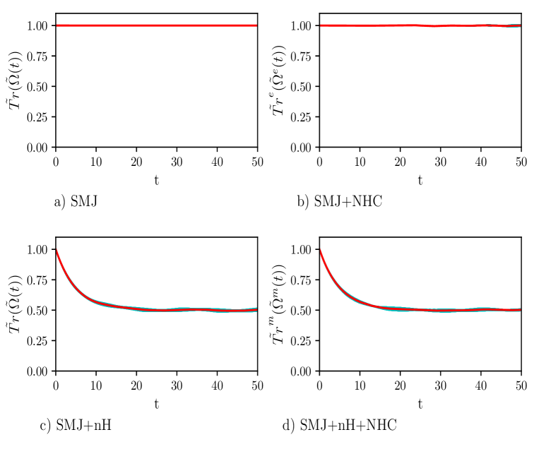
Figure 2: Plot of $\tilde{\rm T}{\rm r}(\tilde{\Omega}(t))$. Number of Monte Carlo sampled phase space initial conditions $X^{\rm e}$ points $=2500$, time step $\tau=0.005$, $\gamma=0.1$, $\omega=1/3$, $\Delta=1$, coupling constant $c=0.007$, inverse temperature $\beta=0.0050$. The red line shows the average trend while the cyan area around it, which is hardly visible, displays the statistical error of the calculation. Panels (a) and (b) show the results of the calculations when the dynamics takes place for the isolated single-molecule junction (SMJ) and for the SMJ at constant temperature (SMJ+NHC), respectively. Panel (c) shows the result of the calculation when a decay operator acts onto the SMJ (SMJ+nH). Finally, in Panel (d) all types of dynamics are considered together (SMJ+nH+NHC). It is easy to see that the trace is conserved when the Hamiltonian is Hermitian. Otherwise, the population drops to about one half as the probability is subtracted only from the excited state.

In order to check the numerical scheme, we calculated the evolution in time of $\tilde{\rm T}{\rm r}(\tilde{\Omega}^{\rm m}(t))$. The results are shown in Fig. 2. When the decay operator is set to zero, Panels (a) and (b), the trace of the density matrix is conserved with extremely good numerical precision both when the dynamics is unitary and when the temperature is controlled. This provides a convincing indication that the our algorithm conserves important dynamical invariants. Panels (c) and (d) in Fig. 2 show the decrease in time of $\tilde{\rm T}{\rm r}(\tilde{\Omega}^{\rm m}(t))$ non-unitary dynamics.Moreover, there is no appreciable difference between unitary and constant-temperature dynamics.

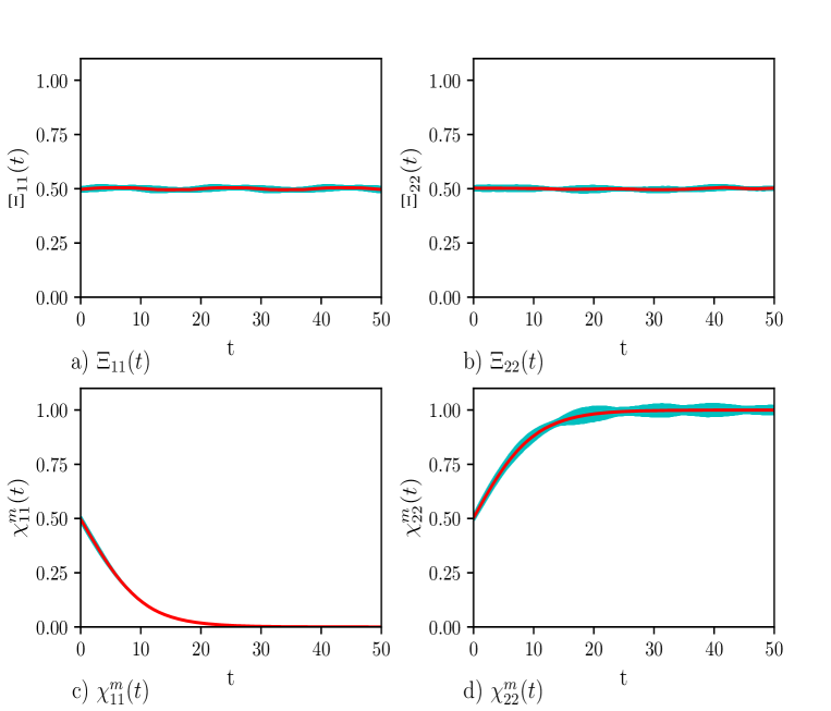
Figure 3: The plots show the diagonal elements of the density matrices resulting from nH+NHC dynamics. Panels (a) and (b) show the behavior of the non-normalized density matrix elements $\Xi_{11}(t)$ and $\Xi_{22}(t)$, respectively. While Panels (c) and (d) display the behavior of the normalized density matrix elements ${\cal X}_{11}^{\rm m}(t)$ and ${\cal X}_{22}^{\rm m}(t)$ . Number of iterations $=10000$, number of Monte Carlo points $=2500$, time step $\tau=0.005$, $\gamma=0.1$, $\omega=1/3$, $\Delta=1$, $c=0.007$, $\beta=0.0050$. The red line is the average trend, the cyan area (almost invisible to the eye) is the error. In (a) the effects of the decay operator $\hat{\Gamma}^{\rm m}$ can be observed. The trend in (b) clarifies the cause for the trend of the trace in Fig.(2). In (c) the difference with (a) is not evident, as the trace decreases directly because of the decrease of $\Omega_{11}$. The comparison between (d) and (b) further clarifies that the cause for the population loss of the excited state is the decay operator and not energy transfer.

In Fig. (3) we show the time-evolution of $\Xi_{\alpha\alpha}^{\rm m}(t)$ and ${\cal X}_{\alpha\alpha}^{\rm m}(t)\rangle^{\rm m}$, with $\alpha=1,2$, defined in Eq. (61) and (62), respectively. Panels (a) and (b) display $\Xi_{11}^{\rm m}(t)$ and $\Xi_{22}^{\rm m}(t)$, respectively. Initially, both adiabatic states are equally occupied. However, according to Eq. (40), only the occupation of the excited state experiences depletion, see in Panel (a). Panels (c) and (d) of Fig. (3) show ${\cal X}_{11}^{\rm m}(t)$ and ${\cal X}_{22}^{\rm m}(t)$, respectively. The behaviour of ${\cal X}_{11}^{\rm m}(t)$ is hardly distinguishable from that of $\Xi_{11}^{\rm m}(t)$. However, the situation is different for ${\cal X}_{22}^{\rm m}(t)$ in Panel (d). As a matter of fact, while $\Xi_{22}^{\rm m}(t)$ is constant, ${\cal X}_{22}^{\rm m}(t)$ increases so that the $\tilde{\rm T}{\rm r}^{\rm m}(\tilde{\rho}^{\rm m}(t))={\cal X}_{11}^{\rm m}(t)+{\cal X}_{22}^{\rm m}(t)=1$.

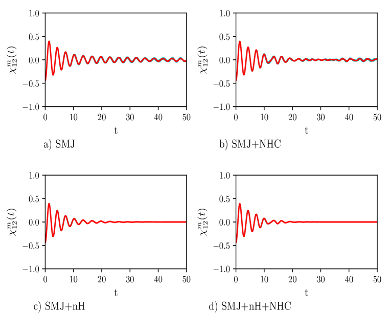
Figure 4: The plot shows the average of the real part of ${\cal X}_{12}^{\rm m}(t)$, the off-diagonal element of the reduced normalized density matrix (NHC+NH system). Number of iterations $=10000$, number of Monte Carlo points $=2500$, time step $\tau=0.005$, $\gamma=0.1$, $\omega=1/3$, $\Delta=1$, $c=0.007$, $\beta=0.0050$. The red line is the average trend, the cyan area is the error. The trend clearly shows decoherence.

In Fig. (4) we show the real part of the reduced off-diagonal element ${\rm Re}({\cal X}_{12}^{\rm m}(t))$. For the chosen values of the parameters, dephasing occurs on the same time scale of the population’s depletion of the excited state.

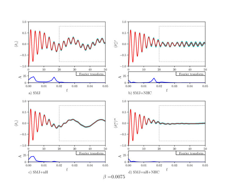
Figure 5: The plot shows the average population transfer vs. time for different types of dynamics. The values of the parameters of the calculation are (NDS=10000, NMCP=2500, $\tau=0.005$, $\gamma=0.1$, $\omega=1/3$, $\Delta=1$, $g=0.007$, $\beta=0.0075$). The red line indicates the average trend, the cyan area represents the error. The blue line denotes the Fourier transform of the time evolution of the average value (the data are considered after $t=20$). Panel (a) displays the results for the isolated SMJ. One can observe that the values oscillate with low and high frequency. Panel (b) displays the dynamics of the SMJ with temperature control (SMJ+NHC). The thermostat facilitates the population transfer and stabilizes its average. The low frequency terms are highly damped while the high frequency ones are unaltered. Panel (c) shows that the effect of the decay operator (SMJ+nH) is to cancel the high frequency term. Finally, in (d), it is shown that the union of the NHC thermostat and decay operator (SMJ+nH+NHC) determines a stable tranfer. Both the low and the high frequency terms are strongly damped.

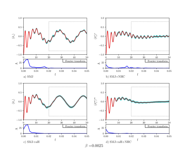
Figure 7: The plot shows the average population transfer vs. time for different types of dynamics. NMDS=10000, NMCP=2500, $\tau=0.005$, $\gamma=0.1$, $\omega=1/3$, $\Delta=1$, $g=0.007$, $\beta=0.0025$. The red line is the average trend, the cyan area is the error. The blue line is the Fourier transform, carried out after the stabilization of the trend (from $t=20$ onward). In Panel (a) the population difference oscillates with low and high frequency contributions (SMJ). Panel (b) shows that the thermostat (SMJ+NHC) facilitates the population transfer and stabilizes it more than in the case of lower temperatures. The low frequency terms are highly damped while the high frequency ones are unaltered. Panel (c) shows that the effect of the decay operator (SMJ+nH) is to cancel the high frequency term. Finally, Panel (d) shows that SMJ+nH+NHC displays a stable transfer: both the low and the high frequency terms are strongly damped.

Figure (5) displays the time evolution of the population difference for $\beta=0.0075$. Below each plot showing the time evolution of the population difference, the Fourier transform is also displayed. The Fourier transform of Panel (a) displays two peaks: one at small frequency and one at higher frequency. The Rabi-like oscillations of the population difference at distant time are signs of the absence of stable quantum transport in the nHQSMJ model. Nosé-Hoover chain dynamics, shown in Panel (b), suppresses the peak at small frequency. The Rabi-like oscillations of the population difference at distant time are less pronounced: they take place at relatively high frequency, as the Fourier transform shows, around zero. This indicates that in the presence of thermal noise the population difference oscillates around zero so that transport is stable. This can be seen as a particular instance of environment-assisted quantum transport: remarkably, the noise provided by an environment can defeat Anderson localization anderson and assist quantum transport. The idea that the noise of the environment could enhance quantum transport, instead of suppressing it, has been postulated to explain the high efficiency of energy transport in photosynthetic systems plenio . Obviously, the noise-enhancement of quantum transport can take place only below a certain threshold. Above it, transport is suppressed by the quantum Zeno effect zeno . In Panel (c) Hamiltonian dynamics of the bath is combined with a non-zero decay operator acting on the two-level system. As it can be seen, the decay operator suppresses the high frequencies in the Rabi-like oscillations of the population difference at distant time. Such oscillations show that, even in this case, quantum transport is not very stable. Comparison of the dynamics in Panel (b) and in Panel (c) shows that there is a difference between thermal and probability sink dissipation: the first suppresses low frequency oscillation while the second damps high frequency oscillations. As one can expect the combination of the two dynamics, shown in Panel (d), leads to the suppression of both frequencies, increasing the efficiency and the stability of the population transport. Calculations for $\beta=0.0025$ are reported in Fig. (7). The results are indistinguishable to the human eye from those obtained at $\beta=0.0075$. This reinforces the conclusion that quantum transport in the nHQSMJ model is enhanced by coupling the two-level system with a probability sink and controlling the temperature of the molecule.

VII Conclusions

In this work, we construct a theory for studying non-Hermitian phase-space-dependent quantum systems at constant temperature. This theory is based on an operator-valued Wigner formulation of quantum mechanics or, in other words, on a phase-space-dependent density matrix. The condition of constant temperature in phase space is achieved by means of the Nosé-Hoover chain thermostat. A mathematical result of the formalism is the derivation of the non-linear equation of motion for the normalized phase-space-dependent density matrix of the system. We remark that this result, considering a constant temperature bath, improves the theory developed in Ref. as_15 where the temperature fluctuations are not constrained. These latter situation is somewhat unrealistic in common experiments.

This theory is applied to a model of a non-Hermitian quantum single-molecule junction. We emphasize that this model treats probability loss and thermal fluctuations on the same level. In detail, the model comprises a two-level system with a probability sink coupled to a thermalized harmonic mode. The structure of our model was conjectured upon drawing an analogy with the process of noise-assisted transport noise ; noise2 ; noise3 . In our case, we expect that the assisted quantum transport arises from the combined action of the probability sink and the constant-temperature fluctuating molecule. Indeed, we observe a transport enhancement in silico upon simulating numerically the non-Hermitian quantum single-molecule junction model for a range of temperatures, while keeping the values of the other parameters constant. The Fourier transformed signal in frequency space shows that the Nosé-Hoover chain thermostat suppresses the slow frequencies while the probability sink damps the high frequency oscillations of the population difference of the non-Hermitian quantum single-molecule junction model at constant temperature.

The non-Hermitian quantum single-molecule junction model at constant temperature introduced in this paper can more accurately be classified as a particular instance of a class of models. As a matter of fact, it can be easily generalized by considering a greater number of quantum states ($\sim 10$) and an even greater number of classical modes ($\sim 10^{3}-10^{5}$). Of course, more sophisticated algorithms would have to be used for calculating the evolution of the density matrix. We also note that spin models that are similar but simpler than the non-Hermitian quantum single-molecule junction model introduced in this paper can be solved analytically when obeying certain symmetry properties hn_16 ; gv_17 ; gm_17 ; gm_18 ; gm_19 ; gv_19 ; gv2_19 ; hn_18 ; hn2_18 . It would be interesting to investigate whether the extension of these models to non-Hermitian quantum mechanics would still be analytically treatable. We defer such generalizations to future work.

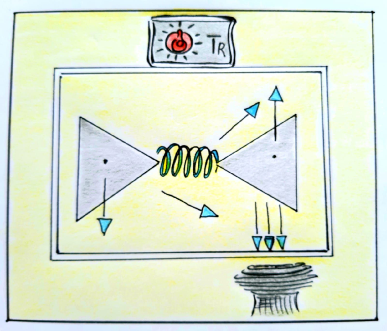
Figure 1: Pictorial representation of the nHQSMJ model. The leads are represented by two gray triangles. The spring portrays the molecule connecting the leads. The arrows with the cyan cusps depict the state of the TLS, depending on its position along the junction. When the TLS is in the left lead, the arrow points downward. As the TLS moves toward the right lead, the arrow rotates until it reaches the upward position, which implies a complete transfer to the right lead. The sink below the right lead absorbs the TLS probability in an irreversible way. In the formalism, the sink is represented by a Hermitian decay operator. The decay operator acts on quantum states that in turn determine probabilities. Hence, the action of the sink unfolds upon an ensemble of trajectories of the TLS system. The picture also shows a box separating the molecular junction from the environment. The drawing of the box resembles on purpose that of an oven with a thermostat on top. The thermostat temperature is set at the same value of the $T_{\rm R}$ temperature of the environment. The thermostat controls the temperature inside the oven so that it is equal to that of the environment. The yellow color inside the oven and around it, in the environment, conveys the idea of thermal equilibrium.

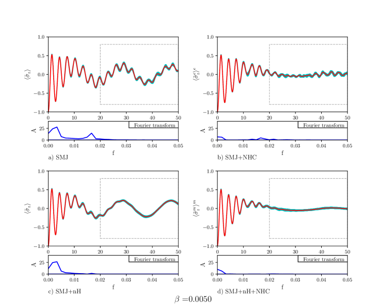
Figure 6: The plot shows the average population transfer vs. time for different types of dynamics. The values of the parameters of the calculation are (NMDS= 10000, NMCP = 2500, $\tau=0.005$, $\gamma=0.1$, $\omega$ = 1/3, $\Delta$ = 1, g = 0.007, $\beta$ = 0.0050). The red line indicates the average trend, the cyan area represents the error. The blue line denotes the Fourier transform of the time evolution of the average value (the data are considered after $t=20$). Panel (a) displays an average population transfer for the SMJ model where low frequency oscillations are strongly damped. In Panel (b) it is shown that a higher temperature damps high frequency oscillations (SMJ+NHC). Statistical error appears to be somewhat greater. Panel (c) shows that the effect of the decay operator is to damp high frequency oscillations (SMJ+nH). Panel (d) shows that the combined action of the NHC thermostat and the decay operator (SMJ+nH+NMJ) determines a stable transfer process. Both low and high frequency oscillations are strongly damped, except for a very weak oscillation at a very low frequency.

Funding: This research received no external funding.

Acknowledgments: AM and AS express their thanks to Hiromichi Nakazato for carefully reading the manuscript and for numerous stimulating suggestions. All the authors are grateful to Dr. Marika Matalone for drawing Figure 1.

Appendix A Time evolution of the trace of $\tilde{\Omega}(t)$

The trace of Eq. (11):

$$\frac{d}{dt}\tilde{\rm T}{\rm r}\left(\tilde{\Omega}(t)\right) = -2\tilde{\rm T}{\rm r}\left(\hat{\Gamma}\tilde{\Omega}(X,t)\right)+\frac{1}{2}\tilde{\rm T}{\rm r}\left(\left\{\tilde{H}^{\rm e},\tilde{\Omega}(t)\right\}_{\mbox{\boldmath$\cal B$}}\right)$$ (63)

$$- \frac{1}{2}\tilde{\rm T}{\rm r}\left(\left\{\tilde{\Omega}(t),\tilde{H}\right\}_{\mbox{\boldmath$\cal B$}}\right)\;.$$

The last term in the right hand side of Eq. (63) can be transformed as follows

$$-\frac{1}{2}\tilde{\rm T}{\rm r}\left(\left\{\tilde{\Omega}(t),\tilde{H}\right\}_{\mbox{\boldmath$\cal B$}}\right) = -\frac{1}{2}\tilde{\rm T}{\rm r}\left(\sum_{I,J=1}^{2N}\frac{\partial\tilde{\Omega}(t)}{\partial X_{I}}{\cal B}_{IJ}\frac{\partial\tilde{H}}{\partial X_{J}}\right)=-\frac{1}{2}\tilde{\rm T}{\rm r}\left(\sum_{I,J=1}^{2N}\frac{\partial\tilde{\Omega}(t)}{\partial X_{J}}{\cal B}_{JI}\frac{\partial\tilde{H}}{\partial X_{I}}\right)$$ (64)

$$= \frac{1}{2}\tilde{\rm T}{\rm r}\left(\sum_{I,J=1}^{2N}\frac{\partial\tilde{H}}{\partial X_{I}}{\cal B}_{IJ}\frac{\partial\tilde{\Omega}(t)}{\partial X_{J}}\right)=\frac{1}{2}\tilde{\rm T}{\rm r}\left(\left\{\tilde{H},\tilde{\Omega}(t)\right\}_{\mbox{\boldmath$\cal B$}}\right)$$

Substituting Eq. (64) in the right hand side of Eq. (63), one obtains

$$\frac{d}{dt}\tilde{\rm T}{\rm r}\left(\tilde{\Omega}(t)\right) = -2\tilde{\rm T}{\rm r}\left(\hat{\Gamma}\tilde{\Omega}(X,t)\right)+\tilde{\rm T}{\rm r}\left(\left\{\tilde{H},\tilde{\Omega}(t)\right\}_{\mbox{\boldmath$\cal B$}}\right)\;.$$ (65)

However, the last term in the right hand side of Eq. (65) is zero:

$$\tilde{\rm T}{\rm r}\left(\left\{\tilde{H},\tilde{\Omega}(t)\right\}_{\mbox{\boldmath$\cal B$}}\right) = \tilde{\rm T}{\rm r}\left(\sum_{I,J=1}^{2N}\frac{\partial\tilde{H}}{\partial X_{I}}{\cal B}_{IJ}\frac{\partial\tilde{\Omega}(t)}{\partial X_{J}}\right)=-\tilde{\rm T}{\rm r}\left(\sum_{I,J=1}^{2N}\frac{\partial^{2}\tilde{H}}{\partial X_{I}\partial X_{J}}{\cal B}_{IJ}\tilde{\Omega}(t)\right)$$ (66)

$$= 0$$

because of the antisymmetry of $\cal B$. Equation (66) allows one to obtain Eq. (15).

Appendix B Time evolution of the trace of $\tilde{\Omega}^{\rm e}(t)$

The trace of Eq. (26) is

$$\frac{d}{dt}\tilde{\rm T}{\rm r}^{\rm e}\left(\tilde{\Omega}^{\rm e}(t)\right)=-2\tilde{\rm T}{\rm r}^{\rm e}\left(\hat{\Gamma}\tilde{\Omega}^{\rm e}(t)\right)+\frac{1}{2}\tilde{\rm T}{\rm r}^{\rm e}\left(\left\{\tilde{H}^{\rm e},\tilde{\Omega}^{\rm e}\right\}_{\mbox{\boldmath$\cal B$}^{\rm e}}\right)-\frac{1}{2}\tilde{\rm T}{\rm r}^{\rm e}\left(\left\{\tilde{\Omega}^{\rm e},\tilde{H}^{\rm e}\right\}_{\mbox{\boldmath$\cal B$}^{\rm e}}\right)-\tilde{\rm T}{\rm r}^{\rm e}\left(\kappa^{\rm e}\tilde{\Omega}^{\rm e}(t)\right)\;.$$ (67)

One can find the following identity

$$\tilde{\rm T}{\rm r}^{\rm e}\left(\left\{\tilde{\Omega}^{\rm e},\tilde{H}^{\rm e}\right\}_{\mbox{\boldmath$\cal B$}^{\rm e}}\right) = \tilde{\rm T}{\rm r}^{\rm e}\left(\sum_{I,J=1}^{2(N+2)}\frac{\partial\tilde{\Omega}^{\rm e}}{\partial X_{I}^{\rm e}}{\cal B}_{IJ}^{\rm e}\frac{\partial\tilde{H}^{\rm e}}{\partial X_{J}^{\rm e}}\right)=\tilde{\rm T}{\rm r}^{\rm e}\left(\sum_{I,J=1}^{2(N+2)}\frac{\partial\tilde{\Omega}^{\rm e}}{\partial X_{J}^{\rm e}}{\cal B}_{JI}^{\rm e}\frac{\partial\tilde{H}^{\rm e}}{\partial X_{I}^{\rm e}}\right)$$ (68)

$$= \tilde{\rm T}{\rm r}^{\rm e}\left(\sum_{I,J=1}^{2(N+2)}\frac{\partial\tilde{H}^{\rm e}}{\partial X_{I}^{\rm e}}{\cal B}_{JI}^{\rm e}\frac{\partial\tilde{\Omega}^{\rm e}}{\partial X_{J}^{\rm e}}\right)=-\tilde{\rm T}{\rm r}^{\rm e}\left(\sum_{I,J=1}^{2(N+2)}\frac{\partial\tilde{H}^{\rm e}}{\partial X_{I}^{\rm e}}{\cal B}_{IJ}^{\rm e}\frac{\partial\tilde{\Omega}^{\rm e}}{\partial X_{J}^{\rm e}}\right)$$

$$= -\tilde{\rm T}{\rm r}^{\rm e}\left(\left\{\tilde{H}^{\rm e},\tilde{\Omega}^{\rm e}\right\}_{\mbox{\boldmath$\cal B$}^{\rm e}}\right)$$

Inserting Eq. (68) in Eq. (67) one obtains

$$\frac{d}{dt}\tilde{\rm T}{\rm r}^{\rm e}\left(\tilde{\Omega}^{\rm e}(t)\right)=-2\tilde{\rm T}{\rm r}^{\rm e}\left(\hat{\Gamma}\tilde{\Omega}^{\rm e}(t)\right)+\tilde{\rm T}{\rm r}^{\rm e}\left(\left\{\tilde{H}^{\rm e},\tilde{\Omega}^{\rm e}\right\}_{\mbox{\boldmath$\cal B$}^{\rm e}}\right)-\tilde{\rm T}{\rm r}^{\rm e}\left(\kappa^{\rm e}\tilde{\Omega}^{\rm e}(t)\right)\;.$$ (69)

One can now find the following identity:

$$\tilde{\rm T}{\rm r}^{\rm e}\left(\left\{\tilde{H}^{\rm e},\tilde{\Omega}^{\rm e}\right\}_{\mbox{\boldmath$\cal B$}^{\rm e}}\right) = -\tilde{\rm T}{\rm r}^{\rm e}\left(\left\{\tilde{H}^{\rm e},\tilde{\Omega}^{\rm e}\right\}_{\mbox{\boldmath$\cal B$}^{\rm e}}\right)=-\tilde{\rm T}{\rm r}^{\rm e}\left(\sum_{I,J=1}^{2(N+1)}\frac{\partial\tilde{H}^{\rm e}}{\partial X_{I}^{\rm e}}{\cal B}_{IJ}^{\rm e}\frac{\partial\tilde{\Omega}^{\rm e}}{\partial X_{J}^{\rm e}}\right)$$ (70)

$$= \tilde{\rm T}{\rm r}^{\rm e}\left(\sum_{I,J=1}^{2(N+1)}\frac{\partial{\cal B}_{IJ}^{\rm e}}{\partial X_{J}^{\rm e}}\frac{\partial\tilde{H}^{\rm e}}{\partial X_{I}^{\rm e}}\tilde{\Omega}^{\rm e}\right)=\tilde{\rm T}{\rm r}^{\rm e}\left(\kappa^{\rm e}\tilde{\Omega}^{\rm e}\right)\;.$$

Equation (70) is obtained exploiting the identity

$$\sum_{I,J=1}^{2(N+1)}{\cal B}_{IJ}^{\rm e}\frac{\partial^{2}\tilde{H}^{\rm e}}{\partial X_{I}^{\rm e}\partial X_{J}^{\rm e}}\equiv 0\;,$$ (71)

which derives from the fact that the trace of a symmetric matrix times an antisymmetric matrix is identically zero. Finally, substituting Eq. (70) in Eq. (69), one obtains Eq. (28).

References

• (1) Ratner, M. A brief history of molecular electronics. Nature Nanotechnology 2013, 8, 378.
• (2) Thoss, M.; Evers, F. Perspective: Theory of quantum transport in molecular junctions. J. Chem. Phys. 2018, 148, 030901.
• (3) Sergi, A.; Hanna, G.; Grimaudo, R.; Messina, A. Quasi-Lie Brackets and the Breaking of Time-Translation Symmetry for Quantum Systems Embedded in Classical Baths. Symmetry 2018, 10, 518.
• (4) Zhang, W. Y.; Balescu, R. Statistical Mechanics of a spin-polarized plasma. J. Plasma Phys. 1988, 40, 199.
• (5) Balescu, R.; Zhang, W. Y. Kinetic equation, spin hydrodynamics and collisional depolarization rate in a spin polarized plasma. J. Plasma Phys. 1988, 40, 215.
• (6) Carpio-Martínez, P.; Hanna, G. Nonequilibrium heat transport in a molecular junction: A mixed quantum-classical approach. J. Chem. Phys. 2019, 151, 074112.
• (7) Gamow, G. Zur Quantentheorie des Atomkernes. Zeitschrift fur Physik 1928, 51, 204–212.
• (8) Bender, C. M. PT Symmetry: In Quantum And Classical Physics, World Scientific: London, 2019.
• (9) Mostafazadeh, A. Pseudo-Hermiticity versus PT symmetry: The necessary condition for the reality of the spectrum of a non-Hermitian Hamiltonian. J. Math. Phys. 2002, 43, 205–214.
• (10) Subotnik, J. E.; Hansen, T.; Hansen, M. A.; Nitzan, A. Nonequilibrium steady state transport via the reduced density matrix operator. J. Chem. Phys. 2009, 130, 144105.
• (11) Zelovich, T.; Kronik, L.; Hod, O. State Representation Approach for Atomistic Time-Dependent Transport Calculations in Molecular Junctions. J. Chem. Theory and Computation 2014, 10, 2927.
• (12) Zelovich, T.; Hansen, T.; Liu, Z.-F.; Neaton, J. B.; Kronik, L.; Hod, O. Parameter-free driven-von Neumann approach electronic transport simulations in open quantum systems. J. Chem. Phys. 2017, 146, 092331.
• (13) Moiseyev, N. Non-Hermitian quantum mechanics. Cambridge University Press: Cambridge, Great Britain, 2011.
• (14) Rotter, I.; Bird, J. P. A review of progress in the physics of open quantum systems: theory and experiment. Reports on Progress in Physics 2015, 78, 114001.
• (15) Sergi, A. Embedding quantum systems with a non-conserved probability in classical environments, Theor. Chem. Acc. 2015, 134, 79.
• (16) Sergi, A.; Zloshchastiev, K. G. Non-Hermitian Quantum Dynamics of a Two-Level System and Models Of Dissipative Environments. International Journal of Modern Physics B 2013, 27, 1350163.
• (17) Sergi, A.; Zloshchastiev, K. G. Time correlation functions for non-Hermitian quantum systems. Phys. Rev. A 2015, 91, 062108.
• (18) Sergi, A.; Zloshchastiev, K. G. Quantum entropy of systems described by non-Hermitian Hamiltonians. JSTAT 2016, 3, 033102.
• (19) Sergi A.; Giaquinta, P. V. Linear Quantum Entropy and Non-Hermitian Hamiltonians. Entropy 2016, 18, 451(11pp).
• (20) Grimaudo, R.; de Castro, A. S. M.; Kuś, M.; Messina, A. Exactly solvable time-dependent pseudo-Hermitian su(1,1) Hamiltonian models. Phys. Rev. A 2018, 98, 033835.
• (21) Zloshchastiev, Konstantin G. Quantum-statistical approach to electromagnetic wave propagation and dissipation inside dielectric media and nanophotonic and plasmonic waveguides. Phys. Rev. B 2016, 94, 115136.
• (22) Zloshchastiev, K. G. Sustainability of Environment-Assisted Energy Transfer in Quantum Photobiological Complexes. Ann. Phys. 2017, 529, 1600185.
• (23) Feshbach, H. Ann. Phys. 1958, 5, 357.
• (24) Feshbach, H. Ann. Phys. 1962, 19, 287.
• (25) Grimaudo, R.; Messina, A.; Sergi, A.; Vitanov, N.; Filippov, S. Two-qubit entanglement generation through non-Hermitian Hamiltonians induced by repeated measurements on an ancilla. Entropy 2020, 22, 1184(1-18).
• (26) Berfield, J. P.; Ratner, M. A. Forty years of molecular electronics: Non-equilibrium heat and charge transport at the nanoscale. Phys. Status Solidi B 2013, 250, 2249.
• (27) Kamenetska, M.; Widawsky, J. R.; Dell’Angela, M.; Frei, M. Temperature dependent tunneling conductance of single molecule junctions. J. Chem. Phys. 2017, 146, 092311.
• (28) G. T. Craven and A. Nitzan, Electron transfer at thermally heterogeneous molecule-metal interfaces. J. Chem. Phys. 146 092305 (2017).
• (29) Sergi A.; Petruccione, F. Nosé-Hoover dynamics in quantum phase space. Journal of Physics A 2008, 41, 355304(14pp).
• (30) Martyna, G. J.; Klein, M. L.; Tuckerman, M. Nosé-Hoover chains: The canonical ensemble via continuous dynamics. J. Chem. Phys. 1992, 97, 2635.
• (31) Sergi, A.; Mac Kernan, D.; Ciccotti, G.; Kapral, R. Simulating Quantum Dynamics in Classical Environments. Theor. Chem. Acc. 2003, 110, 49-58.
• (32) Mac Kernan, D.; Kapral, R.; Ciccotti, G. Sequential short-time propagation of quantum–classical dynamics. J. Phys. Condens. Matter 2002, 14, 9069–9076.
• (33) Sergi A.; Petruccione, F. Sampling Quantum Dynamics at Long Time. Phys. Rev. E 2010, 81, 032101(4pp).
• (34) Uken, D. A.; Sergi, A.; Petruccione, F. Filtering Schemes in the Quantum-Classical Liouville Approach to Non-adiabatic Dynamics. Phys. Rev. E 2013, 88, 033301(7pp).
• (35) Sergi, A. Non-Hamiltonian Commutators in Quantum Mechanics, Phys. Rev. E 2005, 72, 066125.
• (36) A. Sergi, Deterministic constant-temperature dynamics for dissipative quantum systems. J. Phys. A 2007, 40, F347.
• (37) Mac Kernan, D.; Ciccotti, G.; Kapral, R. Surface-hopping dynamics of a spin-boson system. J. Chem. Phys. 2002, 116, 2346.
• (38) Sergi, A.; Ferrario, M. Non-Hamiltonian Equations of Motion with a Conserved Energy. Phys. Rev. E 2001, 64, 056125.
• (39) Sergi, A. Non-Hamiltonian Equilibrium Statistical Mechanics. Phys. Rev. E 2003, 67, 021101.
• (40) Sergi, A.; Giaquinta, P. V. On the geometry and entropy of non-Hamiltonian phase space. JSTAT 2007, 02, P02013(20pp).
• (41) Anderson, P. W. Phys. Rev. 1958, 109, 1492.
• (42) Huelga, S.; Plenio, M. Contemporary Physics 2013, 54, 181.
• (43) Sudarshan, E. C. G.; Misra, B. The Zeno’s paradox in quantum theory. J. Math. Phys. 1977, 18, 756.
• (44) Caruso, F.; Chin, A. W.; Datta, A.; Huelga, S. F.; Plenio, M. B. Highly efficient energy excitation transfer in light-harvesting complexes: The fundamental role of noise-assisted transport. J. Chem. Phys. 2009, 131, 105106.
• (45) Viciani, S.; Lima, M.; Bellini, M.; Caruso, F. Observation of Noise-Assisted Transport in an All-Optical Cavity-Based Network. Phys. Rev. Lett. 2015, 115, 083601.
• (46) Chin, A. W.; Datta, A.; Caruso, F.; Huelga, S. F.; Plenio, M. B. New Journal of Physics 2010, 12, 065002(16pp).
• (47) Grimaudo, R.; Messina, A.; Nakazato, H. Exactly solvable time-dependent models of two interacting two-level systems. Phys. Rev. A 2016, 94, 022108.
• (48) Grimaudo, R.; Messina, Ivanov, P. A.; Vitanov, N. V. Spin-1/2 sub-dynamics nested in the quantum dynamics of two coupled qutrits, J. Phys. A 2017, 50, 175301.
• (49) Grimaudo, R.; Belousov, Y.; Nakazato, H.; Messina, A. Time evolution of a pair of distinguishable interacting spins subjected to controllable and noisy magnetic fields. Ann. Phys. 2017, 392, 242-259.
• (50) Grimaudo, R.; Lamata, L.; Solano, E.; Messina, A. Cooling of many-body systems via selective interactions. Phys. Rev. A 2018, 98, 042330.
• (51) Grimaudo, R.; Isar, A.; Mihaescu, T.; Ghiu, I.; Messina, A. Dynamics of quantum discord of two coupled spin-1/2’s subjected to time-dependent magnetic fields. Results in Physics 2019, 13, 102147.
• (52) Grimaudo, R.; Vitanov, N. V.; Messina, A. Coupling-assisted Landau-Majorana-Stückelberg-Zener transition in a system of two interacting spin qubits. Phys. Rev. B 2019, 99, 174416.
• (53) R. Grimaudo, N. V. Vitanov, and A. Messina, Landau-Majorana-Stc̈kelberg-Zener dynamics driven by coupling for two interacting qutrit systems, Phys. Rev. B 99, 214406 (2019).
• (54) Suzuki, T.; Nakazato, H.; Grimaudo, R.; Messina, A. Analytic estimation of transition between instantaneous eigenstates of quantum two-level system. Scientific reports 2018, 8 1-7.
• (55) Grimaudo, R.; Magalh$\tilde{\rm a}$es de Castro, A. S.; Nakazato, H.; Messina, A. Classes of Exactly Solvable Generalized Semi-Classical Rabi Systems. Annalen der Physik 2018, 530, 1800198.