Topological holographic quench dynamics in a synthetic dimension

Abstract

The notion of topological phases extended to dynamical systems stimulates extensive studies, of which the characterization of non-equilibrium topological invariants is a central issue and usually necessitates the information of quantum dynamics in both the time and spatial dimensions. Here we combine the recently developed concepts of the dynamical classification of topological phases and synthetic dimension, and propose to efficiently characterize photonic topological phases via holographic quench dynamics. A pseudo spin model is constructed with ring resonators in a synthetic lattice formed by frequencies of light, and the quench dynamics is induced by initializing a trivial state which evolves under a topological Hamiltonian. Our key prediction is that the complete topological information of the Hamiltonian is extracted from quench dynamics solely in the time domain, manifesting holographic features of the dynamics. In particular, two fundamental time scales emerge in the quench dynamics, with one mimicking the Bloch momenta of the topological band and the other characterizing the residue time evolution of the state after quench. For this a dynamical bulk-surface correspondence is obtained in time dimension and characterizes the topology of the spin model. This work also shows that the photonic synthetic frequency dimension provides an efficient and powerful way to explore the topological non-equilibrium dynamics.

I Introduction

Discovery of topological quantum phases has revolutionized the understanding of the fundamental phases of quantum matter and ignited extensive research in condensed matter physics over the past decades Hasan2010 ; Qi2011 ; Yan2012 ; Chiu2016 ; Yan2017 . In addition to the great progresses made for equilibrium phases, the notion of topological phases has been extended to far-from-equilibrium dynamical systems, with novel topological physics being uncovered, such as the anomalous topological states in Floquet systems Rudner2013 ; Hu2015 ; Mukherjee2017 ; Maczewsky2017 ; Wintersperger2020 ; VincentLiu2020 ; Zhang2020PRL and dynamical topology emerging in quantum quenches Caio2015 ; WilsonPRL2016 ; Hu2016 ; Wang2017 ; Heyl2018 ; Flaschner2018 ; Song2018 ; GongPRL2018 ; McGinley2019 ; QiuX2019 ; Hu2020 ; XiePRL2020 ; Yu2020 ; Lu2019 ; Slager2020 . In particular, a universal dynamical bulk-surface correspondence was predicted when quenching a system across topological transition Zhang2018 ; Zhang2019 ; Zhang2019b ; Zhang2020PRL , showing that the bulk topology of an equilibrium topological phase has a one-to-one correspondence to quench-induced dynamical topological patterns emerging on the lower-dimensional momentum subspaces called band inversion surfaces (BISs). The dynamical bulk-surface correspondence connects the equilibrium topological phases with far-from-equilibrium quantum dynamics, which was further extended to correlated system Zhang2019c , high-order regimes XLYu2020 ; Gong2020 , and to generic slow non-adiabatic quenches LiPRA2020 . This opens the way to characterize equilibrium topological phases by non-equilibrium quench dynamics, and inversely, to classify non-equilibrium quantum dynamics by topological theory, with the experimental studies having been widely reported recently Sun2018b ; Yi2019 ; Wang2019 ; Song2019 ; Ji2020 ; Xin2020 ; Niu2020 ; BChen2021 . The non-equilibrium topological invariants are typically defined via time dimension and momentum space, and their characterization naturally necessitates the information of quantum dynamics in both the time and spatial dimensions.

As an extension of the spatial degree of freedom, the synthetic dimensions r1 ; r2 ; r3 was proposed and opened an intriguing avenue towards quantum simulation of exotic topological physics beyond physical dimensions r4 ; r5 ; YuanNanophotonics . Following the numerous theoretical proposals on synthetic dimensions using different degree of freedoms such as the frequency or the orbital angular momentum of light r6 ; r7 ; r8 ; r9 , and the hyperfine levels of atoms syn-atom-1 , experiments have been recently performed to demonstrate the two-dimensional topological insulator r10 and the Hall ladder r11 in the synthetic space, where the effective magnetic field for photons is generated, and visualize the edge states syn-atom-2 ; syn-atom-3 . Further, the high-dimensional physics can be studied in a photonic platform with lower dimensionality r8 ; r12 ; r13 ; r14 ; r15 ; r16 . More recently, the experimental platforms for generating the synthetic dimension along the frequency axis have also been proposed and demonstrated using the ring resonator r7 ; r8 ; r11 ; r17 ; Li2020 , in which the photonic modes at equally-spanned frequencies are coupled through the dynamic modulation. In this system, the band structure in the synthetic dimension can be measured in the static steady-state regime in the experiment r17 . On the other hand, with the synthetic dimensions the novel optical phenomena and applications have been be proposed, including the realizations of unidirectional frequency translation s1 , pulse narrowing s2 , active photon storage s3 , and topological laser s4 .

In this work, we combine the concepts of dynamical classification and the synthetic dimension, and propose a highly efficient scheme to characterize topological phases by holographic quench dynamics. We construct a one-dimensional pseudo spin model in a photonic synthetic lattice formed by frequencies of light, and investigate the quench dynamics by initializing a trivial phase which evolves under a topological Hamiltonian. We show that the full dynamical evolution is featured by two fundamental time scales, with which the quench dynamics exhibit universal topological patterns. In particular, one time scale mimics the Bloch momenta of the topological band and the other characterizes the residue time evolution of the state after quench. The dynamical topological patterns obtained on BISs render an emergent dynamical bulk-surface correspondence and provide a holographic characterization of the topological spin model, with the complete information being captured in the single-variable, i.e. the time evolution. The emergent dynamical topology is robust against disorders and has high feasibility in the implementation. This work shows advantages in exploring the topological phases with holographic quench dynamics in the synthetic dimensions, and provides the insight into classifying the far-from-equilibrium dynamics with nontrivial topology based on the synthetic photonic crystals.

II Model

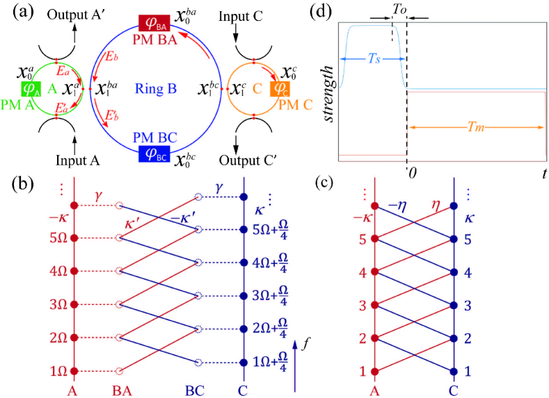
Figure 1: (a) A schematic design of the ring resonator system with phase modulators. External waveguides are used to input (output) signal. (b) The diagram that shows couplings between modes A_m (Red solid dot) and BA_m (Red dashed dot) at frequencies $\omega_{A,m}=m\Omega$ and modes C_m (Blue solid dot) and BC_m (Blue dashed dot) at frequencies $\omega_{C,m}=m\Omega+\Omega/4$. Modulators induce nearest-neighbor couplings (Solid line) between nearby modes along the frequency axis of light, modes in different rings are coupled through the evanescent wave (Dashed line). $\phi_{A}=\phi_{BC}=\pi$ and $\phi_{C}=\phi_{BA}=0$ in modulators give negative (Red line) and positive (Blue line) couplings, respectively. (c) The effective tight-binding model of the pseudo-spin lattice in the nontrivial case ($\phi=\pi$). (d) Time sequences of input source ($T_{S}$) and modulation ($T_{m}$) in simulations. $T_{O}$ is the turn-on/-off time.

We start with illustrating our idea of using ring resonators under dynamic modulations to artificially engineer a tight-binding lattice of pseudo spin states along the frequency axis of light. As shown in Fig. 1(a), the system under the study in this work contains three ring resonators, with each hosting a set of resonant frequency modes. Two of the resonators (A and C) will be used to mimic a pseudospin-$1/2$ system. Let the group velocity be zero in the waveguide that constructs the ring. We set that the ring A supports a set of resonant modes at frequencies $\omega_{A,m}=m\Omega$, where $m$ is an integer and $\Omega=2\pi c/Ln_{g}$ is the free-spectral-range of the ring. Here $c$ is the speed of light, $L$ is the circumference of the ring A, and $n_{g}$ is the effective refractive index. The resonant modes in the ring C with the same circumference $L$ have frequencies: $\omega_{C,m}=m\Omega+\Omega/4$. We use a ring B with the circumference $4L$ to serve as an auxiliary ring r28 . The ring B have shifted resonant modes at frequencies $\omega_{B,m}=m\Omega/4+\Omega/8$. Hence, though there are evanescent couplings between nearby rings, the field resonantly circling inside the ring A(C) is not resonant in the auxiliary ring B.

The couplings between the ring resonators are engineered by properly setting the phase modulators. We place one phase modulator [labelled as PM A(C) in Fig. 1(a)] inside the ring A(C). The light that transmits through the modulator in the ring A(C) undergoes dynamical modulation with the transmission coefficient as a2 :

$$T_{A(C)}=e^{i2\kappa\cos[\Omega_{0}t+\phi_{A(C)}]},$$ (1)

where $\kappa$ is the modulation strength, $\Omega_{0}$ is the modulation frequency, and $\phi_{A(C)}$ is the modulation phase in the modulator PM A(C). We consider the resonant modulation, i.e., $\Omega_{0}=\Omega$, so each modulator couples the nearest-neighbor resonant modes in two rings in the first-order approximation. The ring B contains two phase modulators, which are labelled as PM BA and PM BC with the corresponding transmission coefficients $T_{1}$ and $T_{2}$:

$$T_{1(2)}=e^{i2\kappa^{\prime}\cos(\Omega_{1(2)}t+\phi_{BA(BC)})},$$ (2)

where $\kappa^{\prime}$ is the modulation strength, $\Omega_{1,2}$ are the modulation frequencies, and $\phi_{BA}$ and $\phi_{BC}$ are modulation phases in PM BA and PM BC, respectively. We set $\Omega_{1}=5\Omega/4$ so that the field component at the frequency $\omega_{A,m}$ couples with the component at $\omega_{C,m+1}$. Similarly, for $\Omega_{2}=3\Omega/4$ the component at $\omega_{A,m+1}$ couples with the component at $\omega_{C,m}$.

The pseudospin-$1/2$ system is realized by modulating the resonator couplings. The field in the ring A(C) is coupled with the field in the ring B through the evanescent wave. The corresponding coupling equation is described by the coupling matrix between input electric field amplitudes $E_{a}$, $E_{b}$ and output amplitudes $E_{a}^{\prime}$ and $E_{b}^{\prime}$ labelled in Fig. 1(a):

$$\begin{pmatrix}E_{a}^{\prime}\\ E_{b}^{\prime}\end{pmatrix}=\begin{pmatrix}\sqrt{1-\gamma^{2}}&-i\gamma\\ -i\gamma&\sqrt{1-\gamma^{2}}\end{pmatrix}\begin{pmatrix}E_{a}\\ E_{b}\end{pmatrix}.$$ (3)

Here $\gamma$ is the coupling strength. The coupling matrix between B and C rings follows the same expression. With the above ingredients we can map the setting to the diagram described in Fig. 1(b) which gives our lattice model as shown below. Here, the description of external waveguides used for the input source and output detections in simulations are not included.

The coupling between resonant modes in rings A and C are mediated by the ring B, as illustrated in Fig. 1(b). The physics is described below. The energies of the resonant modes A_m leak into the temporary non-resonant component (labelled as BA_m) in the ring B, which may decay quickly. However, the modulations characterized in Eq. (2) in the ring B convert the energies in these components BA_m to other non-resonant components (labelled as BC_m), and the latter components are transferred to resonant modes C_m in the ring C. Hence the couplings to the auxiliary ring B serve as an intermediate process which mediates an second-order coupling between resonant modes A_m and C_m. This process mimics the second-order Raman process between two states through virtual transitions to an intermediate state in quantum mechanics. On the other hand, the resonant modes with frequencies $\omega_{A,m}$ (labelled as A_m) in the ring A couples between each other through the dynamic modulation characterized in Eq. (1), forming a synthetic lattice for A itself in the frequency dimension, similar for resonant modes C_m) in the ring C.

We now turn to the effective model of the coupled ring system. The modulations including modulation phases inside rings have high tunability r28 . We choose modulation phases to be either $0$ or $\pi$. For example, we can set $\phi_{A}=\phi_{BC}=\pi$, which gives the corresponding negative coupling, or $\phi_{C}=\phi_{BA}=0$, which gives the positive corresponding coupling. The system can be described by an effective Hamiltonian:

$$H = \sum\limits_{m}{{\omega_{A,m}}a_{m}^{\dagger}{a_{m}}+{\omega_{C,m}}c_{m}^{\dagger}{c_{m}}+2\kappa[\cos(\Omega t+\phi)(a_{m}^{\dagger}{a_{m+1}}+a_{m+1}^{\dagger}{a_{m}})}$$ (4)

$$+\cos(\Omega t)(c_{m}^{\dagger}{c_{m+1}}+c_{m+1}^{\dagger}{c_{m}})]+2\eta[\cos(5\Omega t/4)(a_{m}^{\dagger}{c_{m+1}}+c_{m+1}^{\dagger}{a_{m}})$$

$$+\cos(3\Omega t/4+\phi)(c_{m}^{\dagger}{a_{m+1}}+a_{m+1}^{\dagger}c_{m})],$$

where $a$ ($a^{\dagger}$) and $c$ ($c^{\dagger}$) are the annihilation (creation) operators for resonant modes A_m and C_m in rings A and C, respectively, $\eta=\kappa^{\prime}\gamma^{2}$ for the weakly coupling case, and $\phi$ can be either $\pi$ or $0$, depending on what model we are going to study. For the case of $\phi=\pi$, it corresponds to the diagram shown in Fig. 1(c). The Hamiltonian can be rewritten under the rotating-wave approximation:

$$H_{r} = \sum\limits_{m}[e^{i\phi}\kappa(a_{m}^{\dagger}a_{m+1}+a_{m+1}^{\dagger}a_{m})+\kappa(c_{m}^{\dagger}c_{m+1}+c_{m+1}^{\dagger}c_{m})$$ (5)

$$+\eta(a_{m}^{\dagger}c_{m+1}+c_{m+1}^{\dagger}a_{m})+e^{i\phi}\eta(c_{m}^{\dagger}a_{m+1}+a_{m+1}^{\dagger}c_{m})].$$

Eq. (5) with $\phi=\pi$ describes a topological Hamiltonian of a one-dimensional pseudospin-$1/2$ lattice model (with the modes A and C denoting the spin-up and spin-down, respectively) along the synthetic frequency dimension as shown in Fig. 1(c) Zhang2019b . In the following we proceed to study the quench dynamics, and shall show how the dynamical topological patterns emerge in a nontrivial way from simulations.

III Simulation

We perform simulations using the realistic model based on the setting in Fig. 1(a). The simulation has been used to successfully describe the dynamics of the ring-based system in the synthetic space and is discussed in details in Refs r7 ; s1 ; r28 . Here we briefly summarize the procedure. The electric field inside the waveguide is b1

$$E(t,r_{\perp},x)=\sum_{m}\mathcal{E}(t,x)E_{m}(r_{\perp})e^{i\omega^{\prime}_{m}t},$$ (6)

where $x$ is the propagation direction along the waveguide that composes the ring resonator, $r_{\perp}$ is the perpendicular directions of $x$, $\omega^{\prime}_{m}$ is either $\omega_{A,m}$ or $\omega_{C,m}$, $E_{m}(r_{\perp})$ is the modal profile for the ring A or C as well as the auxillary ring B, and $\mathcal{E}(t,x)$ is the associated modal amplitude in different rings. Under the slowly varying envelope approximation, Eq. (6) satisfies the wave equation:

$$[\frac{\partial}{\partial x}+i\beta(\omega^{\prime}_{m})]\mathcal{E}_{m}-\frac{n_{g}}{c}\frac{\partial}{\partial t}\mathcal{E}_{m}=0,$$ (7)

where $\beta$ is the wavevector. The ring has the periodic boundary condition $\mathcal{E}_{m}(t,x+L)=\mathcal{E}_{m}(t,x)$ for rings A and C, and $\mathcal{E}_{m}(t,x+4L)=\mathcal{E}_{m}(t,x)$ for the ring B.

When the light passes through the phase modulation, the field undergoes dynamic modulation and modal amplitudes obey b2 :

$$\mathcal{E}_{m}^{A/C}(t^{+},x_{0}^{a/c})=J_{0}(\kappa)\mathcal{E}_{m}^{A/C}(t^{-},x_{0}^{a/c})+J_{1}(\kappa)\mathcal{E}_{m-1}^{A/C}(t^{-},x_{0}^{a/c})e^{i\phi_{A/C}}-J_{1}(\kappa)\mathcal{E}_{m+1}^{A/C}(t^{-},x_{0}^{a/c})e^{-i\phi_{A/C}},$$ (8)

where $t^{\pm}=t+0^{\pm}$, $x_{0}^{a/c}$ represents the position of the modulator in the ring A or C in Fig. 1(a), and $J_{0}$ and $J_{1}$ are the $0$th and $1$st order Bessel functions, respectively. Here we take the first-order approximation and only consider the nearest-neighbor couplings, which turns out to be fine in this model and also in other works for weak modulations r7 ; s1 ; r28 . Similarly, dynamic modulations on both PM BA and PM BC at positions $x_{0}^{ba}$ and $x_{0}^{bc}$, respectively, are described by following equations:

$$\mathcal{E}_{m}^{BA(BC)}(t^{+},x_{0}^{ba(bc)})=J_{0}(\kappa^{\prime})\mathcal{E}_{m}^{BA(BC)}(t^{-},x_{0}^{ba(bc)})-J_{1}(\kappa^{\prime})\mathcal{E}_{m+1}^{BC(BA)}(t^{-},x_{0}^{ba(bc)})e^{-i\phi_{BA(BC)}},$$ (9)

Eqs. (8) and (9) reflect transmission coefficients in Eqs. (1) and (2), respectively. The coupling in Eq. (3) between fields in rings A and B through the evanescent wave at corresponding positions in Fig. 1(a) can be described by:

$$\mathcal{E}_{m}^{A(BA)}(t^{+},x_{1}^{a(ba)})=\sqrt{1-\gamma^{2}}\mathcal{E}_{m}^{A(BA)}(t^{-},x_{1}^{a(ba)})-i\gamma\mathcal{E}_{m}^{BA(A)}(t^{-},x_{1}^{a(ba)}),$$ (10)

The coupling between fields in ring C and ring B is similarly described.

In simulations, the four external waveguides coupling the rings A and C, as shown in Fig. 1(a), are applied to input the source fields (which can also be decomposed to the frequency component $E_{m}^{A,\mathrm{in}}$ and $E_{m}^{C,\mathrm{in}}$) and detect the output signal ($E_{m}^{A,\mathrm{out}}$ and $E_{m}^{C,\mathrm{out}}$). The input/output coupling between the waveguide and the ring is also described by the similar equations (10) with the coupling strength $\gamma^{\prime}$ r28 .

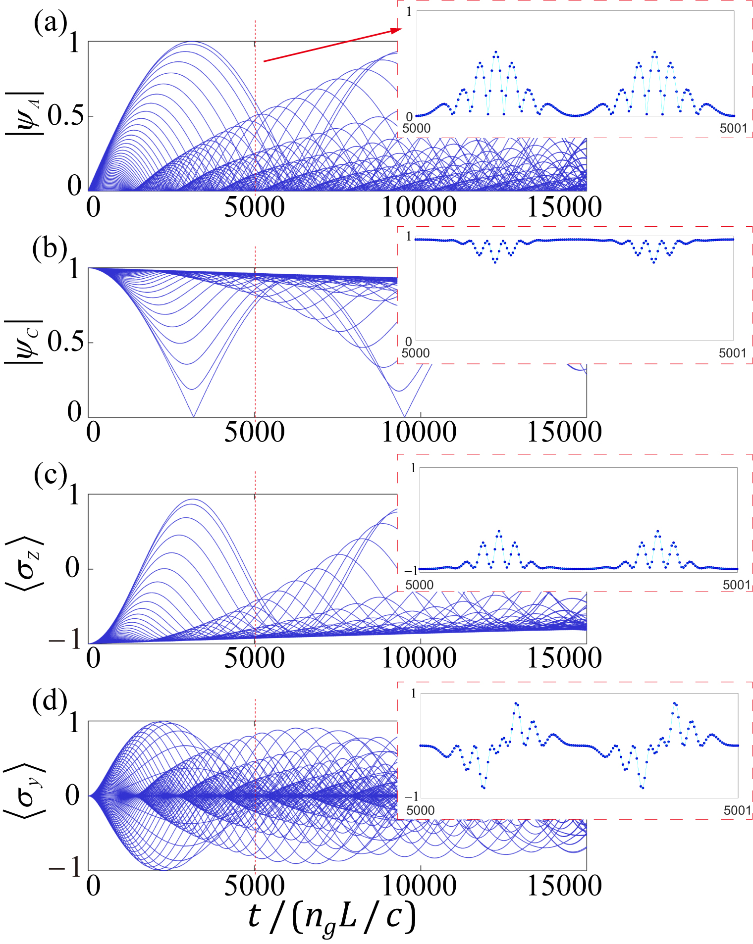
Figure 2: The electric field amplitudes and spin texture from simulations. (a) and (b) The normalized electric field amplitudes $|\psi_{A}|$ and $|\psi_{C}|$ versus discrete time collected from the output waveguides. 160 data points are collected in one roundtrip (=$1\ n_{g}L/c$). (c) and (d) The time evolution of normalized spin textures ($\langle\sigma_{z}\rangle$ and $\langle\sigma_{y}\rangle$). Insets are the corresponding zoom-in plots, where data points are connected with lines, showing that $|\psi_{A}|$, $|\psi_{C}|$, $\langle\sigma_{z}\rangle$, and $\langle\sigma_{y}\rangle$ are evolving continuously along the time dimension.

IV Results and Analysis

IV.1 Simulation results

In this section, we show the feasibility of directly measuring the bulk topology of the system quench dynamics process. To this purpose, we first prepare the initial state of the system by injecting a monochromic light at the center frequency $\omega_{C,0}$ into the input external waveguide C. This source field has the temporal form with a normalized field amplitude $s$

$$E_{0}^{C,\mathrm{in}}=s\{\mathrm{tanh}[0.05(t+t_{S}-t_{O}/2)]+\mathrm{tanh}[0.05(-t_{O}/2-t)]\},$$ (11)

where $t_{O}$ is the turn-on/-off time and $T_{S}$ is the pulse temporal duration. This choice of the input source only excites the mode C_m=0 in the ring C. No mode in the ring A is prepared at $t=0$. Thus the initial excitation of the ring system is fully polarized, giving an initial deep trivial state Zhang2018 . The modulations are then turned on at $t=0$ in the time sequence diagram shown in Fig. 1(d) with the modulation time $T_{m}$. Signals from output external waveguides are collected for further analysis in our simulations. The turning-on of the modulations makes the system be characterized by the non-trivial pseudospin-$1/2$ lattice model described in Fig. 1(c), and the quench dynamics is induced with the initial state evolving under the topological Hamiltanian of Eq. (5).

For the simulation, we set that both ring A and ring C contain 81 resonant modes ($m=-40,-39,...,40$). The parameters designed in the ring resonator system in Fig. 1(a) are: $\kappa=0.0025\ c/Ln_{g}$, $\kappa^{\prime}=0.2\ c/Ln_{g}$, $\gamma=0.1\ c/Ln_{g}$, $\gamma^{\prime}=0.003\ c/Ln_{g}$, respectively. We also choose $T_{S}=1000\ n_{g}L/c$, $T_{O}=200\ n_{g}L/c$, and $T_{m}=15000\ n_{g}L/c$.

Signals are collected from $t=0$ to $t=T_{m}$ for all the frequency components $E_{m}^{A,\mathrm{out}}(t)$ and $E_{m}^{C,\mathrm{out}}(t)$ at both output waveguides. Therefore, the total electric field amplitudes of the signals, $\psi_{A}(t)$ and $\psi_{C}(t)$, can be retrieved by $\psi_{A}(t)=\sum_{m}E_{m}^{A,\mathrm{out}}(t)e^{-i\omega_{A,m}t}$, and $\psi_{C}(t)=\sum_{m}E_{m}^{C,\mathrm{out}}(t)e^{-i\omega_{C,m}t}$. We plot normalized $|\psi_{A}(t)|$ and $|\psi_{C}(t)|$ under the time evolution in Figs. 2(a) and 2(b), respectively, which show nearly periodic patterns over the short time [see the zoom-in plots in both figures]. Nevertheless, the dynamics does not show the periodic stability over a long time, which is an evidence for the steady-state solution of the system r17 . With the collected signal, one can further construct the spin textures $\langle\sigma_{z}(t)\rangle=|\psi_{A}|^{2}-|\psi_{C}|^{2}$ and $\langle\sigma_{y}(t)\rangle=-i\psi_{A}^{*}\cdot\psi_{C}e^{i\Omega t/4}+i\psi_{C}^{*}e^{-i\Omega t/4}\cdot\psi_{A}$, with which we shall show the essential prediction of this work that the two time fundamental scales emerge in the dynamics and the novel topological patterns are resulted (see also Appendix A for details). Time evolution of normalized $\langle\sigma_{z}(t)\rangle$ and $\langle\sigma_{y}(t)\rangle$ are plotted in Figs. 2(c) and 2(d). Note that the raw pseudopsin dynamics characterized by $\langle\sigma_{z}\rangle$ and $\langle\sigma_{y}\rangle$ do not exhibit topological feature explicitly, but actually contain the complete information as presented below.

IV.2 Topological quench dynamics in the synthetic frequency dimension

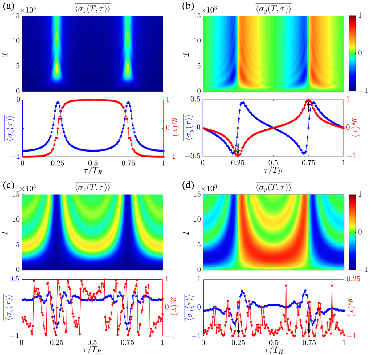
Figure 3: The time evolution of the normalized spin textures reconstructed by using two time scales ($\tau$ and $T$). (a) and (b) The evolution of averaged spin-polarization $\overline{\langle\sigma_{z,y}(T,\tau)\rangle}$, the overall spin-polarization $\overline{\langle\sigma_{z,y}(\tau)\rangle}$, the dynamical spin texture $g_{z,y}(\tau)$, respectively, with $\phi=\pi$. (c) and (d) The evolution of averaged spin-polarization $\overline{\langle\sigma_{z,y}(T,\tau)\rangle}$, the overall spin-polarization $\overline{\langle\sigma_{z,y}(\tau)\rangle}$, the dynamical spin texture $g_{z,y}(\tau)$, respectively, with $\phi=0$. Red arrows point to values of $g_{y}(\tau_{1,2})$.

A novel observation is that two fundamental time scales emerge in the time evolution of the pseudospin polarization, denoted as the slow time variable $T$ and the fast time variable $\tau$, respectively. The real time reads $t=TT_{R}+\tau$, with $T_{R}=2\pi/\Omega$. Thus $T$ is the round-trip numbers, which is a discrete non-negative integer ($T=0,1,2,\ldots$), and $\tau\in[0,T_{R})$ is the round-trip time. Note that for the synthetic dimension along the frequency axis of light, the round-trip time $\tau$ corresponds to the Bloch momentum $k_{f}$, i.e. the wave vector reciprocal to the frequency. For studies modelling a static system, the transmission of light versus $\tau$ at the periodicity $T_{R}$ can give the steady-state bandstructure of the synthetic lattice along the frequency axis of light r11 ; r17 . However, in our present study, the topological quench dynamics is extracted from the two emergent time scales in the time dimension, of which $\tau$ mimics the Bloch momentum and $T$ denotes the residue time evolution of the state.

We therefore represent results $\langle\sigma_{z}(t)\rangle$ and $\langle\sigma_{y}(t)\rangle$ by defining $\langle\sigma_{z}(T,\tau)\rangle$ and $\langle\sigma_{y}(T,\tau)\rangle$, which give the quench dynamics at the Bloch momenta $k_{f}=\tau$ evolving over the discrete residue time $T$. The dynamical classification theory Zhang2018 states that the quench dynamics exhibit nontrivial topology captured by the time-averaged spin texture in momentum space. Unlike the previous theory, here we define the averaged spin-polarization $\overline{\langle\sigma_{z}(T,\tau)\rangle}$ and $\overline{\langle\sigma_{y}(T,\tau)\rangle}$ over the residue time $T$, given by

$$\overline{\langle\sigma_{y,z}(T,\tau)\rangle}=\frac{1}{T+1}\sum_{T^{\prime}=0}^{T}\langle\sigma_{y,z}(T^{\prime},\tau)\rangle.$$ (12)

We show $\overline{\langle\sigma_{y,z}(T,\tau)\rangle}$ and the overall spin-polarization $\overline{\langle\sigma_{y,z}(\tau)\rangle}\equiv\lim_{T\rightarrow\infty}\overline{\langle\sigma_{y,z}(T,\tau)\rangle}$ in Figs. 3(a)-3(c). The plots exhibit nontrivial dynamical pattern characterized via the two time scales $\tau$ and $T$. First, the overall averaged polarizations vanish $\overline{\langle\sigma_{y,z}(\tau)\rangle}=0$ at two special points with $\tau_{1}=0.25T_{R}$ and $\tau_{2}=0.75T_{R}$. Such two characteristic points are known as band inversion points in the 1D Brillouin zone (BZ) Zhang2018 . Secondly, we define a new dynamical spin texture in the following way:

$$\vec{g}(\tau)=\left\{\begin{array}[]{lr}(1/{\cal N})\partial_{\tau}\overline{\langle\vec{\sigma}(\tau)\rangle},\ \ \ \tau=\tau_{1,2};\\ (s/{\cal N})\overline{\langle\vec{\sigma}(\tau)\rangle},\ \ \ \ \ \ \mathrm{other}\ \tau\ \mathrm{points},\end{array}\right.$$ (15)

where $\cal N$ is the normalization factor, the derivative direction is chosen from the area in-between the two band inversion points to that out of them if $\tau$ is at band inversion points, and $s=-1$ ($+1$) if $\tau$ is in the region in-between (out of) the two band inversion points for other $\tau$ points. One finds that at the two band inversion points $g_{z}(\tau_{1,2})=0$, while $g_{y}(\tau_{1})=-g_{y}(\tau_{2})=-1$ points in opposite directions [see Fig. 3(d)], giving a nonzero dynamical topological number, i.e. the zeroth Chern number $C_{0}=[g_{y}(\tau_{2})-g_{y}(\tau_{1})]/2$, as defined via the two band inversion points. This manifests the emergent dynamical bulk-surface correspondence Zhang2018 , and the bulk topology of the Hamiltonian of the synthetic lattice constructed in Fig. 1(c) is topologically nontrivial. As a comparison, we can use the same system but change the modulation phase $\phi=0$, and show the numerical results in Figs. 3(e)-3(h). The emergent dynamical field $\vec{g}(\tau)$ at two band inversion points are the same [Fig. 3(h)], corresponding to the trivial case.

The above results of quench dynamics can be understood from the tight-binding model given in Eq. (5), which further takes the form in the momentum $k$-space

$${H}_{k} = \kappa(a_{k}^{\dagger}a_{k}e^{ikd}e^{i\phi}+a_{k}^{\dagger}a_{k}e^{-ikd}e^{i\phi}+c_{k}^{\dagger}c_{k}e^{ikd}+c_{k}^{\dagger}c_{k}e^{-ikd})$$ (16)

$$+\eta(a_{k}^{\dagger}c_{k}e^{ikd}+a_{k}^{\dagger}c_{k}e^{-ikd}e^{i\phi}+c_{k}^{\dagger}a_{k}e^{-ikd}+c_{k}^{\dagger}a_{k}e^{ikd}e^{i\phi}),$$

with $d$ the lattice constant. For $\phi=\pi$, the above Hamiltonian gives a 1D topological phase known as AIII class insulator and characterized by a 1D winding number Liu2013 ; Song2018 (see also details in Appendix B). The dynamical topological number defined through $\vec{g}(\tau_{1,2})$ in quench dynamics precisely corresponds to the 1D winding number of the above Bloch Hamiltonian. On the other hand, for $\phi=0$ the above Hamiltonian gives a 1D gapless spin-orbit coupled band with trivial topology (see Appendix B).

We emphasize the highly nontrivial features of the topological quench dynamics, which provide the holographic characterization of the topological phase realized in the ring-resonator system, namely, the quench dynamics solely in the time-dimension contains the complete information. The single variable, i.e. the time $t$, automatically splits into two fundamental time scales, mimicking the Bloch momenta $\tau$ of the topological band and the residue time evolution $T$ after quench, respectively, with which the bulk topology of the system is completely determined animation . Specifically, the pseudo spin dynamics averaged over the time scale $T$ manifest BIS structure depicted via $\tau$. The derivative of the $T$-averaged spin dynamics with respect to $\tau$ across BIS points determines the bulk topology. This result is in sharp contrast to the conventional characterization of the non-equilibrium topological invariants, which necessitates the information in both the time dimension and real momentum space. On the other hand, this prediction also shows the novelty of classifying by topological theory the non-equilibrium dynamics, whose raw features are quite complicated and depend on Hamiltonian details (Fig. 2), but are actually classified by the underlying universal topological patterns (Fig. 3) through the characterization scheme given above animation .

V Topological quench dynamics with disorders

V.1 Perturbation of disorder in the phase modulator

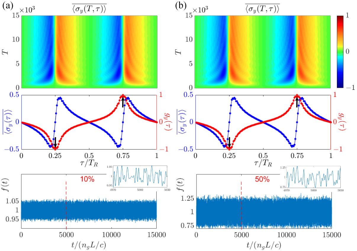
Figure 4: The evolution of averaged spin-polarization $\overline{\langle\sigma_{y}(T,\tau)\rangle}$, the overall spin-polarization $\overline{\langle\sigma_{y}(\tau)\rangle}$, $g_{y}(\tau)$, respectively, with parameters for Fig. 3(a) and 3(b) and disorder function $f(t)$ in $\kappa(t)$ and $\kappa^{\prime}(t)$ with $\delta=10\%$(a) and $50\%$(b), respectively. Red arrows point to values of $g_{y}(\tau_{1,2})$.

In this subsection, we consider the perturbation of topological quench dynamics from disorders in phase modulators. Such disorders in the phase modulation can be reflected in modulation strengths, $\kappa$ and $\kappa^{\prime}$. We consider that $\kappa$ and $\kappa^{\prime}$ undergo a random perturbation continuously, which is varying in time and can be described by $\kappa(t)=\kappa_{0}\cdot f(t)$, $\kappa^{\prime}(t)=\kappa_{0}^{\prime}\cdot f(t)$, where $\kappa_{0}=0.0025\ c/Ln_{g}$ and $\kappa_{0}^{\prime}=0.2\ c/Ln_{g}$. Here $f(t)=1+\delta r(t)$ is the disorder function, where $r(t)$ is a time-varying random function with a range $[-0.5,0.5]$ and $\delta$ represents the disorder intensity.

Simulations are performed with parameters for Figs. 3(a) and 3(b) and $\delta=10\%$ and $50\%$, respectively, and results of $\overline{\langle\sigma_{y}(T,\tau)\rangle}$ together with $\overline{\langle\sigma_{y}(\tau)\rangle}$ and $g_{y}(\tau)$ are plotted in Fig. 4, with the corresponding $f(t)$. Compared to the dynamical pattern in Fig. 3(b), evolutions of $\overline{\langle\sigma_{y}(T,\tau)\rangle}$ with different disorder $\delta$ show relatively similar profiles. The averaged spin-polarization pattern and the nontrivial dynamical spin texture preserve when phase modulators include temporal disorders. This result can be understand since the temporal disorder in $\kappa$ and $\kappa^{\prime}$ does not break the symmetry feature in the Hamiltonian in Eq. (16), and hence the bulk topology of the Hamiltonian preserves.

V.2 Perturbation of disorder in the input source

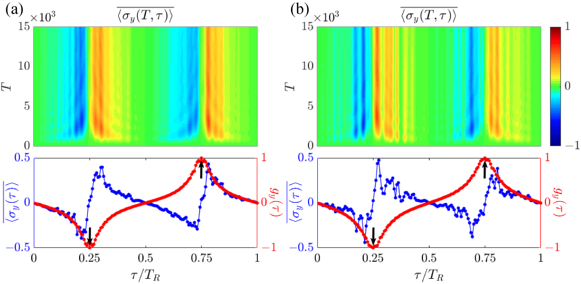
Figure 5: The evolution of averaged spin-polarization $\overline{\langle\sigma_{y}(T,\tau)\rangle}$, the overall spin-polarization $\overline{\langle\sigma_{y}(\tau)\rangle}$, $g_{y}(\tau)$, respectively, with parameters for Figs. 3(a) and 3(b) and disorder in the input source in Eq. (17) with $\delta=5\%$(a) and $10\%$(b), respectively. Red arrows point to values of $g_{y}(\tau_{1,2})$.

In simulation for Figs. 3(a) and 3(b), we prepare the initial state of the system by injecting a monochromic light at the center frequency $\omega_{C,0}$. In this subsection, we consider the injected light has disorder in both intensities and phases for all frequency modes. Such disorder in the input source can be described by

$$\left\{\begin{array}[]{lr}E_{0}^{C,\mathrm{in}}=(1-\delta\cdot R)\cdot s\cdot{\tanh[0.05(t+t_{S}-t_{O}/2)]+\tanh[0.05(-t_{O}/2-t)]},\\ E_{m\neq 0}^{C,\mathrm{in}}=\delta\cdot R\cdot e^{i2\pi R},\ \ \ \ \ \ \ \ \ \ \ \ 0\leqslant t\leqslant t_{s}\end{array}\right.$$ (17)

where $\delta$ is the disorder intensity and $R$ gives a random number in the range $[-0.5,0.5]$.

We perform simulations with same parameters for Figs. 3(a) and 3(b) and the input source in Eq. (17) with $\delta=5\%$ and $10\%$, respectively. The corresponding evolutions of $\overline{\langle\sigma_{y}(T,\tau)\rangle}$ together with $\overline{\langle\sigma_{y}(\tau)\rangle}$ and $g_{y}(\tau)$ are plotted in Fig. 5. Although the disorder in the input source affects more largely the topological quench dynamics for the case with larger $\delta$, the overall spin-polarization in $\overline{\langle\sigma_{y}(\tau)\rangle}$ as well as the nontrivial dynamical spin texture $g_{y}(\tau)$ still capture the topological feature of the studied system.

VI Experimental feasibility

The quench dynamics is induced by initializing a deep trivial phase for the topological Hamiltonian, which in principle has a high experimental feasibility in comparison with the currently achieved band structure measurement for the resonator ring systems r17 ; Li2020 . In the present study, we do not need to prepare the initial system to be in the eigenstates of the Hamiltonian, nor to scan the frequency to match the band energies, which are however required and were the major challenges for the conventional band mapping techniques. This essential difference makes the present quench study be of high feasibility.

Further, the proposed ring resonator system can be achieved in both fiber-based platforms r11 ; r17 ; Li2020 and on-chip lithium niobate photonic designs c2 ; c3 , where the parameters in the system can be realized in experiments. In both systems, the conversion efficiency of the electro-optic modulators can reach up to $\sim 2\%$ c3 ; c4 ; c5 ; c6 , which is sufficient for the proposed system here. The quality factor for the ring is potentially possible at the order of $\sim 10^{7}-10^{8}$ with an amplifier for compensation in fiber rings r11 ; r17 or the state-of-art integrated lithium niobate technology c7 . Therefore, our proposal provides an experimental feasible platform for measuring the quench dynamics and the topological invariants directly from the temporal optical signal in ring resonator, which can lead to significant simplification of performing dynamical characterization of topological quantum phases in different synthetic models.

VII Conclusion and discussion

In summary, we have investigated the topological quench dynamics in a 1D spinful lattice model synthesized in the dimension of frequency of light in ring resonators, and predicted the holographic features of the quench dynamics. In particular, we showed that the quench dynamics in time domain can be generically characterized with two emergent time scales, with one mimicking the Bloch momentum of the lattice and the other characterizing the residue time evolution. In this characterization the quench dynamics, being complicated in the original time dimension, exhibit universal dynamical topological patterns which correspond to the bulk topology of the post-quench Hamiltonian. The topological quench dynamics is robust against disorders and of high feasibility in experimental realization. We note that the approach proposed in this work is generic, and the study can be readily extended to topological phases in synthetic high-dimensions, e.g. to the 2D Haldane model r28 . In that case we expect that the multiple fundamental time scales would emerge in the holographic quench dynamics, with some mimicking the high-dimensional Bloch momenta and the remaining characterizing the residue time evolution, for which the complex quench dynamics can be classified by the exotic dynamical topology and has profound connection to the bulk topology of the post-quench Hamiltonian. This work showed a unique way to study the holographic far-from-equilibrium dynamics, with the rich and complex topological physics being captured in only the single-variable, i.e. the time evolution, and shall provided the insight into the exploration of the high-dimensional topological phases with quench dynamics in the synthetic photonic crystals.

Appendix A Relation between fields and spin textures

Signals collected from output waveguide in Fig. 1(a) in the main text are $\psi_{A}(t)$ and $\psi_{C}(t)$, respectively. Spin textures of the one-dimensional pseudo-spin lattice in Fig. 1(c) in the main text include $\langle\sigma_{z}\rangle$ and $\langle\sigma_{y}\rangle$, respectively. The relation between spin textures $\langle\sigma_{z}\rangle$, $\langle\sigma_{y}\rangle$ and signals $\psi_{A}$, $\psi_{C}$ satisfies:

$$\langle\sigma_{z}\rangle \equiv \begin{pmatrix}\psi_{A}^{*},\psi_{C}^{*}e^{-i\Omega t/4}\end{pmatrix}\begin{pmatrix}1&0\\ 0&-1\end{pmatrix}\begin{pmatrix}\psi_{A}\\ \psi_{C}e^{i\Omega t/4}\end{pmatrix}={\left|{\psi_{A}}\right|^{2}}-{\left|{\psi_{C}}\right|^{2}},$$ (18)

$$\langle\sigma_{y}\rangle \equiv \begin{pmatrix}\psi_{A}^{*},\psi_{C}^{*}e^{-i\Omega t/4}\end{pmatrix}\begin{pmatrix}0&-i\\ i&0\end{pmatrix}\begin{pmatrix}\psi_{A}\\ \psi_{C}e^{i\Omega t/4}\end{pmatrix}$$ (19)

$$= -i\psi_{A}^{*}\cdot\psi_{C}e^{i\Omega t/4}+i\psi_{C}^{*}e^{-i\Omega t/4}\cdot\psi_{A}.$$

Here the extra coefficient $e^{\pm i\Omega t/4}$ is from the frequency offset between rings A and C. It is obvious that Eqs. (S1) and (S2) can be obtained by subtraction of intensities of two optical signals and interference between two optical signals, respectively.

Appendix B Comparison with numerical results from tight-binding models

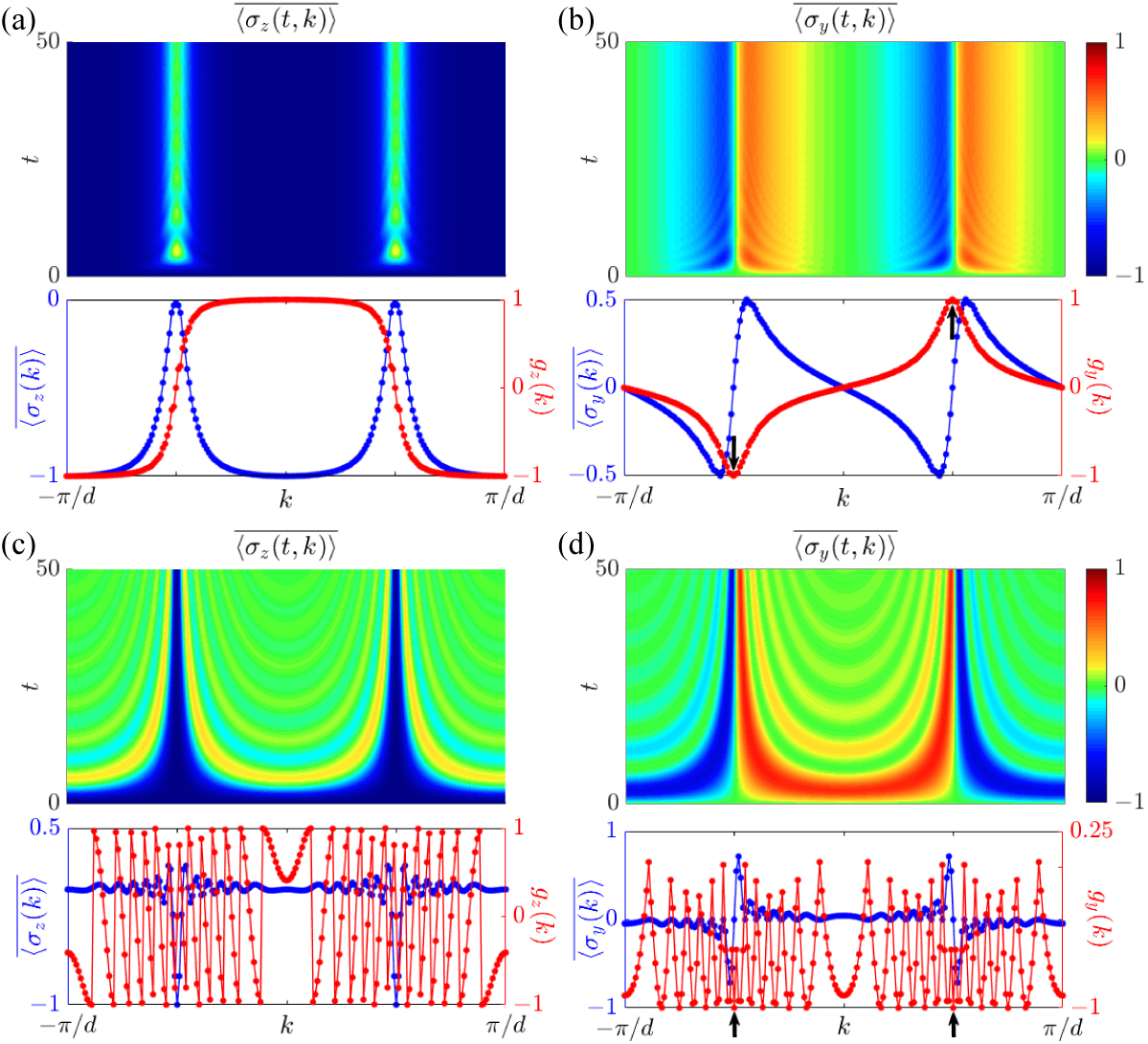
Figure S1: Numerical simulation results of spin textures in the $k$-space. (a) and (b) The evolution of averaged spin-polarization $\overline{\langle\sigma_{z,y}(t,k)\rangle}$, the overall spin-polarization $\overline{\langle\sigma_{z,y}(k)\rangle}$, the dynamical spin texture $g_{z,y}(k)$, respectively, with $\phi=\pi$. (c) and (d) The evolution of averaged spin-polarization $\overline{\langle\sigma_{z,y}(t,k)\rangle}$, the overall spin-polarization $\overline{\langle\sigma_{z,y}(k)\rangle}$, the dynamical spin texture $g_{z,y}(k)$, respectively, with $\phi=0$. Red arrows point to values of $g_{y}(k=\pm\pi/2d)$.

In this section, we show the numerical simulations of the corresponding spin textures by numerically solving the tight-binding model in Eq. (5) in the main text with $\phi=\pi$ or 0, respectively. The Hamiltonian can be re-written in the $k$-space:

$${H}_{k} = \kappa(a_{k}^{\dagger}a_{k}e^{ikd}e^{i\phi}+a_{k}^{\dagger}a_{k}e^{-ikd}e^{i\phi}+c_{k}^{\dagger}c_{k}e^{ikd}+c_{k}^{\dagger}c_{k}e^{-ikd})$$ (20)

$$+\eta(a_{k}^{\dagger}c_{k}e^{ikd}+a_{k}^{\dagger}c_{k}e^{-ikd}e^{i\phi}+c_{k}^{\dagger}a_{k}e^{-ikd}+c_{k}^{\dagger}a_{k}e^{ikd}e^{i\phi}),$$

where $d$ is the lattice constant. One can rewrite Eq. (20) in the momentum space $H_{k}=-2\kappa\cos(kd)\sigma_{z}-2\eta\sin(kd)\sigma_{y}$ when $\phi=\pi$, which gives the 1D AIII class topological insulator with 1D winding number Liu2013 ; Song2018 , and $H_{k}=2\kappa\cos(kd)I+2\eta\cos(kd)\sigma_{x}$ when $\phi=0$. Here $I$ is the unit matrix. The spin textures of the system can then be simulated with initial condition $\langle\sigma_{z}\rangle=-1,\langle\sigma_{y}\rangle=0,\langle\sigma_{x}\rangle=0$, and $\eta=0.2\kappa$.

The simulation results of $\langle\sigma_{z,y}(t,k)\rangle$ for $\phi=\pi$ and $0$ are obtained, and corresponding $\overline{\langle\sigma_{z,y}(t,k)\rangle}$, $\overline{\langle\sigma_{z,y}(k)\rangle}$, and $g_{z,y}(k)$ can be defined in the same procedure as that in the main text and then be plotted in Fig. S1. One can notice that these numerical results give the non-trivial feature for $\phi=\pi$ and trivial feature for $\phi=0$, respectively Zhang2018 . Comparing both results in Fig. 3 in the main text and Fig. S1, one finds the consistency in the quench dynamics which gives the same evidences for either non-trivial or trivial case.

References

- (1) M. Z. Hasan and C. L. Kane, Colloquium: Topological insulators, Rev. Mod. Phys. 82, 3045-3067 (2010).
- (2) X.-L. Qi and S.-C. Zhang, Topological insulators and superconductors, Rev. Mod. Phys. 83, 1057-1110 (2011).
- (3) B. Yan and S.-C. Zhang, Topological materials, Rep. Prog. Phys. 75, 096501 (2012).
- (4) C.-K. Chiu, J. C. Y. Teo, A. P. Schnyder, and S. Ryu, Classification of topological quantum matter with symmetries, Rev. Mod. Phys. 88, 035005 (2016).
- (5) B. Yan and C. Felser, Topological Materials: Weyl Semimetals, Annu. Rev. Condens. Matter Phys. 8, 337-354 (2017).
- (6) M. S. Rudner, N. H. Lindner, E. Berg, and M. Levin, Anomalous Edge States and the Bulk-Edge Correspondence for Periodically Driven Two-Dimensional Systems, Phys. Rev. X 3, 031005 (2013).
- (7) W. Hu, J. C. Pillay, K. Wu, M. Pasek, P. Ping Shum, and Y. D. Chong, Anomalous Edge States and the Bulk-Edge Correspondence for Periodically Driven Two-Dimensional Systems, Phys. Rev. X 5, 011012 (2015).
- (8) S. Mukherjee, A. Spracklen, M. Valiente, E. Andersson, P. Öhberg, N. Goldman, and R. R. Thomson, Experimental observation of anomalous topological edge modes in a slowly driven photonic lattice, Nat. Commun. 8, 13918 (2017).
- (9) L. J. Maczewsky, J. M. Zeuner, S. Nolte, and A. Szameit, Observation of photonic anomalous Floquet topological insulators, Nat. Commun. 8, 13756 (2017).
- (10) K. Wintersperger, C. Braun, F. N. Ünal, A. Eckardt, M. Di Liberto, N. Goldman, I. Bloch, M. Aidelsburger, Realization of an anomalous Floquet topological system with ultracold atoms, Nature Phys. 16, 1058-1063 (2020).
- (11) H. Hu, B. Huang, E. Zhao, and W. V. Liu, Dynamical Singularities of Floquet Higher-Order Topological Insulators. Phys. Rev. Lett. 124, 057001 (2020).
- (12) L. Zhang, L. Zhang, and X.-J. Liu, Unified Theory to Characterize Floquet Topological Phases by Quench Dynamics, Phys. Rev. Lett. 125, 183001 (2020).
- (13) M. D. Caio, N. R. Cooper, and M. J. Bhaseen, Quantum Quenches in Chern Insulators, Phys. Rev. Lett. 115, 236403 (2015).
- (14) Y. Hu, P. Zoller, and J. C. Budich, Dynamical Buildup of a Quantized Hall Response from Nontopological States, Phys. Rev. Lett. 117, 126803 (2016).
- (15) J.H. Wilson, J.C.W. Song, and G. Rafael, Remnant Geometric Hall Response in a Quantum Quench, Phys. Rev. Lett. 117, 235302 (2016).
- (16) C. Wang, P. Zhang, X. Chen, J. Yu, and H. Zhai, Scheme to Measure the Topological Number of a Chern Insulator from Quench Dynamics, Phys. Rev. Lett. 118, 185701 (2017).
- (17) M. Heyl, Dynamical quantum phase transitions: A review, Rep. Prog. Phys. 81, 054001 (2018).
- (18) N. Fläschner, D. Vogel, M. Tarnowski, B. S. Rem, D. S. Lühmann, M. Heyl, J. C. Budich, L. Mathey, K. Sengstock, and C. Weitenberg, Observation of dynamical vortices after quenches in a system with topology, Nat. Phys. 14, 265-268 (2018).
- (19) B. Song, L. Zhang, C. He, T. F. J. Poon, E. Hajiyev, S. Zhang, X.-J. Liu, and G.-B. Jo, Observation of symmetry-protected topological band with ultracold fermions, Sci. Adv. 4, aao4748 (2018).
- (20) Z. Gong and M. Ueda, Topological Entanglement-Spectrum Crossing in Quench Dynamics, Phys. Rev. Lett. 121, 250601 (2018).
- (21) M. McGinley and N. R. Cooper, Classification of topological insulators and superconductors out of equilibrium, Phys. Rev. B 99, 075148 (2019).
- (22) Y.-H. Lu, B.-Z. Wang, and X.-J. Liu, Ideal Weyl semimetal with 3D spin-orbit coupled ultracold quantum gas, Sci. Bull. 65, 2080-2085 (2020).
- (23) X. Qiu, T.-S. Deng, Y. Hu, P. Xue, and W. Yi, Fixed Points and Dynamic Topological Phenomena in a Parity-Time-Symmetric Quantum Quench, iScience 20, 392-401 (2019).
- (24) D. Xie, T.-S. Deng, T. Xiao, W. Gou, T. Chen, W. Yi, and B. Yan, Topological Quantum Walks in Momentum Space with a Bose-Einstein Condensate, Phys. Rev. Lett. 124, 050502 (2020).
- (25) H. Hu and E. Zhao, Topological Invariants for Quantum Quench Dynamics from Unitary Evolution, Phys. Rev. Lett. 124, 160402 (2020).
- (26) X. Chen, C. Wang, and J. Yu, Linking invariant for the quench dynamics of a two-dimensional two-band Chern insulator, Phys. Rev. A 101, 032104 (2020).
- (27) F. Nur Ünal, A. Bouhon, and R.-J. Slager, Topological Euler Class as a Dynamical Observable in Optical Lattices, Phys. Rev. Lett. 125, 053601 (2020).
- (28) L. Zhang, L. Zhang, S. Niu, and X.-J. Liu, Dynamical classification of topological quantum phases, Sci. Bull. 63, 1385-1391 (2018).
- (29) L. Zhang, L. Zhang, and X.-J. Liu, Dynamical detection of topological charges, Phys. Rev. A 99, 053606 (2019).
- (30) L. Zhang, L. Zhang, and X.-J. Liu, Characterizing topological phases by quantum quenches: A general theory, Phys. Rev. A 100, 063624 (2019).
- (31) L. Zhang, L. Zhang, Y. Hu, N. Sen, and X.-J. Liu, Emergent topology and symmetry-breaking order in correlated quench dynamics, arXiv:1903.09144 (2019).
- (32) X.-L. Yu, L. Zhang, J. Wu, X.-J. Liu, High-order band inversion surfaces in dynamical characterization of topological phases, arXiv:2004.14930 (2020).
- (33) L. Li, W. Zhu, and J. Gong, Topological characterization of higher-order topological insulators with nested band inversion surfaces, arXiv:2007.05759 (2020).
- (34) J. Ye and F. Li, Emergent topology under slow nonadiabatic quantum dynamics, Phys. Rev. A 102, 042209 (2020).
- (35) W. Sun, C.-R. Yi, B.-Z. Wang, W.-W. Zhang, B. C. Sanders, X.-T. Xu, Z.-Y. Wang, J. Schmiedmayer, Y. Deng, X.-J. Liu, S. Chen, and J.-W. Pan, Uncover Topology by Quantum Quench Dynamics, Phys. Rev. Lett. 121, 250403 (2018).
- (36) Y. Wang, W. Ji, Z. Chai, Y. Guo, M. Wang, X. Ye, P. Yu, L. Zhang, X. Qin, P. Wang, F. Shi, X. Rong, D. Lu, X.-J. Liu, and J. Du, Experimental observation of dynamical bulk-surface correspondence in momentum space for topological phases, Phys. Rev. A 100, 052328 (2019).
- (37) C.-R. Yi, L. Zhang, L. Zhang, R.-H. Jiao, X.-C. Cheng, Z.-Y. Wang, X.-T. Xu, W. Sun, X.-J. Liu, S. Chen, and J.-W. Pan, Observing Topological Charges and Dynamical Bulk-Surface Correspondence with Ultracold Atoms, Phys. Rev. Lett. 123, 190603 (2019).
- (38) B. Song, C. He, S. Niu, L. Zhang, Z. Ren, X.-J. Liu, and G.-B. Jo, Observation of nodal-line semimetal with ultracold fermions in an optical lattice, Nat. Phys. 15, 911-916 (2019).
- (39) W. Ji, L. Zhang, M. Wang, L. Zhang, Y. Guo, Z. Chai, X. Rong, F. Shi, X.-J. Liu, Y. Wang, and J. Du, Quantum Simulation for Three-Dimensional Chiral Topological Insulator, Phys. Rev. Lett. 125, 020504 (2020).
- (40) T. Xin, Y. Li, Y.-a. Fan, X. Zhu, Y. Zhang, X. Nie, J. Li, Q. Liu, and D. Lu, Quantum Phases of Three-Dimensional Chiral Topological Insulators on a Spin Quantum Simulator, Phys. Rev. Lett. 125, 090502 (2020).
- (41) J. Niu, T. Yan, Y. Zhou, Z. Tao, X. Li, W. Liu, L. Zhang, S. Liu, Z. Yan, Y. Chen, and D. Yu, Simulation of Higher-Order Topological Phases and Related Topological Phase Transitions in a Superconducting Qubit, arXiv:2001.03933 (2020).
- (42) B. Chen, S. Li, X. Hou, F. Ge, F. Zhou, P. Qian, F. Mei, S. Jia, N. Xu, and H. Shen, Digital quantum simulation of Floquet topological phases with a solid-state quantum simulator, Photonics Research 9, 81-87 (2021).
- (43) D. I. Tsomokos, S. Ashhab, and F. Nori, Using superconducting qubit circuits to engineer exotic lattice systems, Phys. Rev. A 82, 052311 (2010).
- (44) O. Boada, A. Celi, J. I. Latorre, and M. Lewenstein, Quantum Simulation of an Extra Dimension, Phys. Rev. Lett. 108, 133001 (2012).
- (45) D. Juki and H. Buljan, Four-dimensional photonic lattices and discrete tesseract solitons, Phys. Rev. A 87, 013814 (2013).
- (46) L. Yuan, Q. Lin, M. Xiao, and S. Fan, Synthetic dimension in photonics, Optica 5, 1936 (2018).
- (47) T. Ozawa, H. M. Price, A. Amo, N. Goldman et al, Topological photonics, Rev. Mod. Phys. 91, 015006 (2019).
- (48) D. Leykam, and L. Yuan, Topological phases in ring resonators: recent progress and future prospects, Nanophotonics 9, 4473 (2020).
- (49) X. -W. Luo, X. Zhou, C. -F. Li, J. -S. Xu et al, Quantum simulation of 2D topological physics in a 1D array of optical cavities, Nat. Commun. 6, 7704 (2015).
- (50) L. Yuan, Y. Shi, and S. Fan, Photonic gauge potential in a system with a synthetic frequency dimension, Opt. Lett. 41, 741-744 (2016).
- (51) T. Ozawa, H. M. Price, N. Goldman, O. Zilberberg, and I. Carusotto, Synthetic dimensions in integrated photonics: From optical isolation to four-dimensional quantum Hall physics, Phys. Rev. A 93, 043827 (2016).
- (52) L. Yuan, Q. Lin, A. Zhang, M. Xiao, X. Chen, and S. Fan, Photonic Gauge Potential in One Cavity with Synthetic Frequency and Orbital Angular Momentum Dimensions, Phys. Rev. Lett. 122, 083903(2019).
- (53) A. Celi, P. Massignan, J. Ruseckas, N. Goldman, I. B. Spielman, G. Juzelinas, and M. Lewenstein, Synthetic Gauge Fields in Synthetic Dimensions, Phys. Rev. Lett. 112, 043001 (2014).
- (54) E. Lustig, S. Weimann, Y. Plotnik, Y. Lumer, M. A. Bandres, A. Szameit, and M. Segev, Photonic Topological Insulator in Synthetic Dimensions, Nature 576, 356-360 (2019).
- (55) A. Dutt, Q. Lin, L. Yuan, M. Minkov, M. Xiao, and S. Fan, A single photonic cavity with two independent physical synthetic dimensions, Science 367, 59-64 (2020).
- (56) M. Mancini, G. Pagano, G. Cappellini, L. Livi, M. Rider, J. Catani, C. Sias, P. Zoller, M. Inguscio, M. Dalmonte, and L. Fallani, Observation of chiral edge states with neutral fermions in synthetic Hall ribbons, Science 349, 1510-1513 (2015).
- (57) B. K. Stuhl, H.-I. Lu, L. M. Aycock, D. Genkina, and I. B. Spielman, Visualizing edge states with an atomic Bose gas in the quantum Hall regime, Science 349, 1514-1518 (2015).
- (58) Q. Lin, M. Xiao, L. Yuan, and S. Fan, Photonic Weyl point in a two-dimensional resonator lattice with a synthetic frequency dimension, Nat. Commun. 7, 13731 (2016).
- (59) Q. Lin, X. -Q. Sun, M. Xiao, S. -C. Zhang, and S. Fan, A three-dimensional photonic topological insulator using a two-dimensional ring resonator lattice with a synthetic frequency dimension, Sci. Adv. 4, eaat2774 (2018).
- (60) B. A. Bell, K. Wang, A. S. Solntsev, D. N. Neshev, A. A. Sukhorukov, and B. J. Eggleton, Spectral photonic lattices with complex long-range coupling, Optica 4, 1433-1436 (2017).
- (61) C. Qin, F. Zhou, Y. Peng, D. Sounas, X. Zhu, B. Wang, J. Dong, X. Zang, A. Al, and P. Lu, Spectrum Control through Discrete Frequency Diffraction in the Presence of Photonic Gauge Potentials, Phys. Rev. Lett. 120, 133901 (2018).
- (62) L. J. Maczewsky, K. Wang, A. A. Dovgiy, A. E. Miroshnichenko, A. Moroz, M. Ehrhardt, M. Heinrich, D. N. Christodoulides, A. Szameit, and A. A. Sukhorukov, Synthesizing multi-dimensional excitation dynamics and localization transition in one-dimensional lattices, Nat. Photonics 14, 76-81 (2020).
- (63) A. Dutt, M. Minkov, Q. Lin, L. Yuan, D. A. B. Miller, and S. Fan, Experimental band structure spectroscopy along a synthetic dimension, Nat. Commun. 10, 3122 (2019).
- (64) G. Li, Y. Zheng, A. Dutt, D. Yu, Q. Shan, S. Liu, L. Yuan, S. Fan, and X. Chen, Dynamic band structure measurement in the synthetic space, Sci. Adv. 7 eabe4335 (2021).
- (65) L. Yuan, and S. Fan, Bloch oscillation and unidirectional translation of frequency in a dynamically modulated ring resonator, Optica 3, 1014-1018 (2016)
- (66) L. Yuan, Q. Lin, M. Xiao, A. Dutt, and S. Fan, Pulse shortening in an actively mode-locked laser with parity-time symmetry, APL Photonics 3, 086103 (2018).
- (67) D. Yu, L. Yuan, and X. Chen, Isolated Photonic Flatband with the Effective Magnetic Flux in A Synthetic Space including the Frequency Dimension, Laser Photonics Rev. 14, 2000041 (2020).
- (68) Z. Yang, E. Lustig, G. Harari, Y. Plotnik, Y. Lumer, M. A. Bandres, and M. Segev, Mode-Locked Topological Insulator Laser Utilizing Synthetic Dimensions, Phys. Rev. X 10, 011059 (2020).
- (69) L. Yuan, M. Xiao, Q. Lin, and S. Fan, Synthetic space with arbitrary dimensions in a few rings undergoing dynamic modulation, Phys. Rev. B 97, 104105 (2018).
- (70) A. Yariv and P. yeh, Photonics: Optical Electronics in Modern Communications (Oxford University, New York, 2007).
- (71) H. A. Haus, Waves and Fields in Optoelectronics (Prentice-Hall, Inc., Englewood Cliffs, NJ, 1984).
- (72) B. E. A. Saleh and M. C. Teich, Fundamentals of Photonics (Wiley-Interscience, Hoboken, NJ, 2007).
- (73) X.-J. Liu, Z.-X. Liu, and M. Cheng, Manipulating Topological Edge Spins in a One-Dimensional Optical Lattice, Phys. Rev. Lett. 110, 076401 (2013).
- (74) See Supplemental Material at http://link.aps.org/supplemental/…, which includes a cartoon illustrating how the bulk topology of the system can be completely determined from the information of quench dynamics solely in the time dimension.
- (75) M. Zhang, C. Wang, Y. Hu, A. Shams-Ansari, T. Ren, S. Fan, M. Lonar, Electronically programmable photonic molecule, Nat. Photonics 13, 36-40 (2019).
- (76) C. Wang, M. Zhang, X. Chen, M. Bertrand, A. Shams-Ansari, S. Chandrasekhar, P. Winzer, and M. Lonar, Integrated lithium niobate electro-optic modulators operating at CMOS-compatible voltages, Nature 562, 101-104 (2018).
- (77) L. D. Tzuang, K. Fang, P. Nussenzveig, S. Fan, and M. Lipson, Non-reciprocal phase shift induced by an effective magnetic flux for light, Nat. Photonics 8, 701-705 (2014).
- (78) C. Wang, M. Zhang, B. Stern, M. Lipson, and M. Lonar, Nanophotonic lithium niobate electro-optic modulators, Opt. Express 26, 1547-1555 (2018).
- (79) C. Reimer, Y. Hu, A. Shams-Ansari, M. Zhang, and M. Lonar, High-dimensional frequency crystals and quantum walks in electro-optic microcombs, arXiv:1909.01303 (2019).
- (80) B. Desiatov, A. Shams-Ansari, M. Zhang, C. Wang, and M. Lonar, Ultra-low-loss integrated visible photonics using thin-film lithium niobate, Optica 6, 380-384 (2019).