Spin and charge transport through helical Aharonov-Bohm interferometer with strong magnetic impurity

Abstract

We discuss transport through an interferometer formed by helical edge states of the quantum spin Hall insulator. Focusing on effects induced by a strong magnetic impurity placed in one of the arms of interferometer, we consider the experimentally relevant case of relatively high temperature as compared to the level spacing. We obtain the conductance and the spin polarization in the closed form for arbitrary tunneling amplitude of the contacts and arbitrary strength of the magnetic impurity. We demonstrate the existence of quantum effects which do not show up in previously studied case of weak magnetic disorder. We find optimal conditions for spin filtering and demonstrate that the spin polarization of outgoing electrons can reach 100%.

I Introduction

A novel class of materials — topological insulators — has become a hot topic in the last decade. These materials are insulating in the bulk, but exhibit conducting states at the edges of the sample Bernevig and Hughes (2013); Hasan and Kane (2010); Qi and Zhang (2011). The edge states demonstrate surprising properties. In particular, in two-dimensional (2D) topological insulators (TI) edge states are one-dimensional channels where: (i) the electron spin is tightly connected to the electron motion direction, e.g. electrons with spin-up and spin-down propagate in opposite directions; (ii) the electron transport is ideal, in the sense that electrons do not experience backscattering from conventional non-magnetic impurities, similarly to what occurs in edge states of Quantum Hall Effect, but without invoking high magnetic fields. The 2D topological insulator phase was predicted in HgTe quantum wells Kane and Mele (2005); Bernevig et al. (2006) and confirmed by direct measurements of conductance of the edge states König et al. (2007) and by the experimental analysis of the non-local transport Roth et al. (2009); Gusev et al. (2011); Brüne et al. (2012); Kononov et al. (2015).

Considerable attention was paid to the analysis of the Aharonov Bohm (AB) effect in 2D TI: the dependence of the longitudinal conductance of nanoribbons and nanowires on the magnetic flux piercing their cross-section was studied Peng et al. (2010); Lin et al. (2017); weak antilocalization was investigated in the disordered topological insulators and oscillations with magnetic flux with the period equal to the half of the flux quantum were predicted Bardarson et al. (2010); Bardarson and Moore (2013). The AB effect was discussed for almost closed loops formed by curved edge states Delplace et al. (2012). Also, the AB oscillations were observed in the magnetotransport measurements of transport (both local and nonlocal) in 2D topological insulators based on HgTe quantum wells Gusev et al. (2015) and were explained by coupling of helical edges to bulk puddles of charged carriers.

The purpose of the current paper is to study standard AB setup based on helical-edge states (HES) of a quantum spin Hall insulator tunnel-coupled to leads (see Fig. 1).

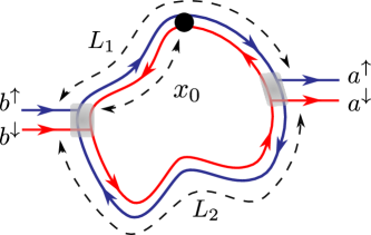
Figure 1: Helical Aharonov-Bohm interferometer with the magnetic impurity placed in the upper shoulder.

Such an interferometer was already studied theoretically at zero temperature Chu et al. (2009); Masuda and Kuramoto (2012); Dutta et al. (2016). Here, we focus on the case of relatively high temperature, $T\gg\Delta,$ where $\Delta=2\pi v_{F}/L$ is the level spacing which is controlled by total edge length $L=L_{1}+L_{2},$ where $L_{1,2}$ are lengths of the interferometer’s shoulders. For typical sample parameters, $L=10~{}\mu$m and $v_{F}=10^{7}$ cm/s, we estimate the level spacing $\Delta\approx 3$ K. As seen from this estimate, the case $T\gg\Delta$ is interesting for possible applications. There is also upper limitation for temperature. For good quantization, $T$ should be much smaller than the bulk gap of the topological insulator: $T\ll\Delta_{\rm b}$. For the first time quantum spin Hall effect was observed in structures based on HgTe/CdTe Konig et al. (2007) and InAs/GaSb Knez et al. (2011), which had a rather narrow bulk gap, less than 100 K. Substantially large values were observed recently in WTe${}_{2},$ where gap of the order of 500 K was observed Wu et al. (2018), and in bismuthene grown on a SiC (0001) substrate, where a bulk gap of about 0.8 eV was demonstrated Reis et al. (2017); Li et al. (2018) (see also recent discussion in Ref. Stühler et al. (2020)). Thus, recent experimental studies unambiguously indicate the possibility of transport through HES at room temperature, when the condition

$$\Delta_{\rm b}\gg T\gg\Delta$$ (1)

can be easily satisfied.

The high-temperature regime, $T\gg\Delta,$ was already studied for single-channel AB interferometers made of conventional materials Jagla and Balseiro (1993); Dmitriev et al. (2010); Shmakov et al. (2013); Dmitriev et al. (2015, 2017) and it was demonstrated that flux-sensitive interference effects survive in this case. Recently, we discussed high-temperature electron and spin transport in AB interferometers based on helical edge states of TI Niyazov et al. (2018, 2020). We considered setup shown in Fig. 1 and assumed that there is a weak magnetic impurity (or weak magnetic disorder). We found that both tunneling conductance $G$ and the spin polarization $\mathcal{P}$ of outgoing electrons show sharp resonances appearing periodically with dimensionless flux, $\phi=\Phi/\Phi_{0},$ with the period $\Delta\phi=1/2.$ Here $\Phi$ is the external magnetic flux piercing the area encompassed by edge states and $\Phi_{0}=hc/e$ is the flux quantum. Simple estimates show that condition $\Phi\sim\Phi_{0}$, is achieved for interferometer with HES of typical length $L=10~{}\mu$m in fields $B\sim 3\mbox{ Oe}$, well below the expected magnitude of the fields destroying the edge states Du et al. (2015); Zhang et al. (2014); Hu et al. (2016).

Importantly, condition (1) ensures the universality of spin and charge transport (see discussion in Refs. Niyazov et al. (2018, 2020)), which do not depend on details of the systems, in particular, on the device geometry. A very sharp dependence of the conductance and the spin polarization on $\phi$, predicted in Refs.  Niyazov et al. (2018, 2020), is very promising for applications for tunable spin filtering and in the area of extremely sensitive detectors of magnetic fields. We also demonstrated that charge and spin transfer through the AB helical interferometer can be described in terms of the ensemble of the flux-tunable qubits Niyazov et al. (2020) that opens a wide avenue for high-temperature quantum computing.

In this paper, we generalize the results obtained in Refs. Niyazov et al. (2018, 2020) for the case of a strong impurity. We study electrical and spin transport through AB helical interferometer containing a single magnetic impurity of arbitrary strength and find optimal conditions for spin filtering. We also demonstrate that with increasing of the impurity strength new quantum processes come into play which do not show up for weak impurity. Most importantly, we confirm the idea which was put forward previously Niyazov et al. (2020) but has not yet been verified by direct calculations. We demonstrate that a strong magnetic impurity inserted into one of the interferometer’s shoulder, blocks the transition through this shoulder and only the other shoulder remains active. As a result, the spin polarization of outgoing electrons can achieve 100%. Remarkably, this mechanism is robust to dephasing by a non-magnetic bath, works at high temperatures and thus has high prospects in the quantum computing.

II Model

We consider tunneling charge and spin transport through AB interferometer based on HES. We limit ourselves to a discussion of setup with a single strong impurity placed into the upper shoulder at the distance $x_{0}$ (along the edge) from the left contact (see Fig. 1). We discuss the dependence of the tunneling conductance $G$ and spin polarization of outgoing electrons $\mathcal{P}$ on the external dimensionless magnetic flux $\phi$. Similar to Refs.  Niyazov et al. (2018, 2020), we neglect the influence of the magnetic fields on the helical states.

We assume that the impurity is classical with large magnetic moment $\mathbf{M}$ ($M\gg 1$) and describe such an impurity by the following scattering matrix

$$\hat{S}_{M}=\begin{pmatrix}e^{i\zeta}\cos\theta&i\sin\theta~{}e^{i\varphi}\\ i\sin\theta~{}e^{-i\varphi}&e^{-i\zeta}\cos\theta\\ \end{pmatrix}.$$ (2)

One can show that the forward scattering phase $\zeta$ can be absorbed into the shift of $\phi$ and is put to zero below. We neglect feedback effect related to the dynamics of $\mathbf{M}$ caused by exchange interaction with the ensemble of right- and left-moving electrons Kurilovich et al. (2017) assuming that the direction of $\mathbf{M}$ is controlled, e.g., by in-plane magnetic field, which does not affect the AB interference, or by the magnetic anisotropy of the impurity Hamiltonian. The scattering of electrons may also happen off the ferromagnetic tip placed in the vicinity of HES.

We suppose that HES are tunnel-coupled to metallic leads. These leads are modeled by single-channel spinful wires so that electrons are injected into the helical states through the so-called tunnel Y junctions. Different spin projections do not mix at the tunneling contacts so that electrons entering the edge with opposite spins move in the opposite directions (see Fig. 2). Such contacts are characterized by two amplitudes $r$ and $t,$ obeying $|t|^{2}+|r|^{2}=1.$ We assume that $t$ and $r$ are real and positive and parameterize them as follows:

$$r=\sqrt{1-e^{-2\lambda}},\quad t=e^{-\lambda},\quad 0<\lambda<\infty.$$ (3)

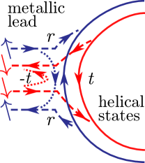
Figure 2: Point contact between the helical edge state and the spinful wire. Blue (red) lines correspond to spin up (down) electrons. Solid lines depict trajectories inside the interferometer. Dashed lines show incoming and outgoing electron trajectories. Dotted lines illustrate reflection by contact.

III Calculation of conductance and polarization

The transmission coefficient, $\mathcal{T}$, the spin transmission coefficient, $\mathcal{T}_{s}$, and the spin polarization, $\mathcal{P}=\mathcal{T}_{s}/\mathcal{T}$, are expressed via the fractions of transmitted electrons, $\mathcal{T}_{\alpha}$, with spin projection $\alpha=\uparrow,\downarrow$. Introducing transfer matrix $\hat{t}$ of the interferormeter as a whole, we get

$$\mathcal{T} =\tfrac{1}{2}({\mathcal{T}_{\uparrow}+\mathcal{T}_{\downarrow}})=\tfrac{1}{2}\left\langle{\rm Tr}\left(\hat{t}\hat{t}^{\dagger}\right)\right\rangle_{\epsilon}\,,$$ (4)

$$\mathcal{T}_{s} =\tfrac{1}{2}\left(\mathcal{T}_{\uparrow}-\mathcal{T}_{\downarrow}\right)=\tfrac{1}{2}\left\langle{\rm Tr}\left(\hat{t}\sigma_{z}\hat{t}^{\dagger}\right)\right\rangle_{\epsilon}\,,$$ (5)

where the thermal averaging, $\langle\cdots\rangle_{\epsilon}=-\int d\epsilon(\cdots)\partial_{\epsilon}f_{F}(\epsilon),$ is performed with the Fermi function $f_{F}(\epsilon).$ Here we assume that the incoming electrons are unpolarized. The tunneling conductance of this setup is given by

$$G=2\frac{e^{2}}{h}\mathcal{T}\,,$$ (6)

where factor $2$ accounts for two conducting channels.

The transfer matrix $\hat{t}$ is defined as follows

$$\begin{pmatrix}a^{\uparrow}\\ a^{\downarrow}\end{pmatrix}=\hat{t}\begin{pmatrix}b^{\uparrow}\\ b^{\downarrow}\end{pmatrix},$$ (7)

where $(b^{\uparrow},b^{\downarrow})$ and $(a^{\uparrow},a^{\downarrow})$ are the amplitudes of incoming (from the left contact) and outgoing (from the right contact) waves, respectively (see Fig. 1). Transfer matrix corresponding to $\hat{S}_{M}$ reads

$$\hat{M}=\frac{1}{\cos\theta}\begin{pmatrix}1&i\sin\theta e^{i\xi}\\ -i\sin\theta e^{-i\xi}&1\end{pmatrix},$$ (8)

where $\xi=\varphi-2kx_{0}$ and $k$ is the electron momentum. The matrix $\hat{t}$ is expressed in terms of $\hat{M}$ as follows Niyazov et al. (2020)

$$\hat{t}= \frac{r^{2}e^{2\pi i\phi L_{1}/L}}{t}\begin{pmatrix}e^{ikL_{1}}&0\\ 0&e^{-ikL_{1}}\end{pmatrix}\begin{pmatrix}t&0\\ 0&1\end{pmatrix}\hat{g}\begin{pmatrix}1&0\\ 0&1/t\end{pmatrix},$$ (9)

$$\hat{g}= \frac{1}{1-e^{2\pi i\phi}\hat{M}\begin{pmatrix}t^{2}e^{ikL}&0\\ 0&e^{-ikL}/t^{2}\end{pmatrix}}\hat{M}\begin{pmatrix}1&0\\ 0&-1\end{pmatrix}.$$

The matrix $\hat{g}$ can be represented as follows

$$\hat{g}=\cos\theta\left[\begin{pmatrix}0&0\\ 0&-1\end{pmatrix}+\sum\limits_{\alpha=\pm}\frac{1+\alpha\hat{H}}{1-t^{2}e^{i(kL+\alpha 2\pi\phi_{0})}}\right],$$ (10)

where $\phi_{0}$ obeys

$$\cos(2\pi\phi_{0})=\cos\theta\cos(2\pi\phi)\,,$$ (11)

and

$$\hat{H}=\begin{pmatrix}a&be^{i\xi}\\ be^{-i\xi}&-a\end{pmatrix}.$$ (12)

The coefficients

$$a=i\frac{e^{-2\pi i\phi}-\cos(2\pi\phi_{0})\cos\theta}{\cos\theta\sin(2\pi\phi_{0})},$$ (13)

$$b=\frac{e^{-2\pi i\phi}\tan\theta}{\sin(2\pi\phi_{0})}$$ (14)

obey $a^{2}+b^{2}=1$ and depend on the strength of the impurity and the magnetic flux only, while the dependence on the energy is encoded in the exponents $e^{\pm i\xi}$ entering off-diagonal terms of $\hat{H}.$

The possibility to express the transmission amplitude $\hat{t}$ in terms of resonance denominators (10) is of primary importance for further high temperature averaging. It allows us to do exact thermal averaging for arbitrary magnetic impurity strength, in the distinction with previous calculations Niyazov et al. (2018, 2020), where perturbative expansion over impurity strength was used for calculation of $\cal T$ and $\cal P$. We first note that the energy dependence in the transfer matrix $\hat{t}$ appears not only in the resonance denominators but also in terms $e^{ikL_{1}}$ and $e^{i2kx_{0}}.$ However, for relevant combinations ${\rm Tr}\left(\hat{t}\hat{t}^{\dagger}\right)$ and ${\rm Tr}\left(\hat{t}\sigma_{z}\hat{t}^{\dagger}\right),$ all energy dependent terms in numerators cancel. It reflects the universality of the HES based interferometers. AB oscillations do not depend on details of the setup: position of the impurity, $x_{0}$, length of the shoulders, $L_{1,2}$, and the Berry phase, $\delta$, as thoroughly discussed in Ref. Niyazov et al. (2018). Thus, we average only the following combinations

$$\left\langle\frac{1}{1-t^{2}e^{i(kL+\alpha 2\pi\phi_{0})}}\frac{1}{1-t^{2}e^{-i(kL+\beta 2\pi\phi_{0})}}\right\rangle_{\epsilon}$$ (15)

$$\qquad=\frac{1}{1-t^{4}e^{(\alpha-\beta)2\pi\phi_{0}}},$$

$$\left\langle\frac{1}{1-t^{2}e^{\pm i(kL+\alpha 2\pi\phi_{0})}}\right\rangle_{\epsilon}=1.$$

Using these formulas, the straightforward algebraic calculation yields

$$\mathcal{T} =\tanh\lambda\left(1-\frac{\sin^{2}\theta\sinh^{2}\lambda\cosh(2\lambda)}{\cosh^{2}(2\lambda)-\cos^{2}\theta\cos^{2}(2\pi\phi)}\right),$$ (16)

$$\mathcal{T}_{s} =-\frac{\sin^{2}\theta\sinh^{2}\lambda\cosh(2\lambda)}{\cosh^{2}(2\lambda)-\cos^{2}\theta\cos^{2}(2\pi\phi)}\,,$$

$$\mathcal{P} =-\frac{\tanh\lambda\sin^{2}\theta}{1+\cos^{2}\theta\left(\tanh^{2}\lambda-\frac{\cos^{2}(2\pi\phi)}{\cosh^{2}\lambda\cosh(2\lambda)}\right)}\,.$$

This is the main result of the current paper. We emphasize that these expressions are valid for arbitrary tunneling amplitude of the contacts, arbitrary strength of the magnetic impurity, and for any magnetic flux.

We see that the transmission coefficient has minima at $\phi=n/2$, and maxima at $\phi=1/4+n/2$ with integer $n$. Instead of $\mathcal{T}(\phi)$ it is convenient to introduce the following normalized function

$$\tau(\phi) =\frac{\mathcal{T}(\phi)-\mathcal{T}(0)}{\mathcal{T}(1/4)-\mathcal{T}(0)}$$ (17)

$$=\frac{\cosh^{2}(2\lambda)\sin^{2}(2\pi\phi)}{\cosh^{2}(2\lambda)-\cos^{2}\theta\cos^{2}(2\pi\phi)}\,.$$

which is plotted in Fig. 3 for four different values of the magnetic impurity strength, $\theta$. Sharp antiresonances structure of $\mathcal{T}(\phi)$ is transforming to an oscillation shape with increasing of $\theta$. Simultaneously, depth of conductance antiresonances is decreasing such that $\mathcal{T}(\phi)\to\text{const}$ for $\theta\to\pi/2$. This case corresponds to the ideal reflection of electrons on the impurity.

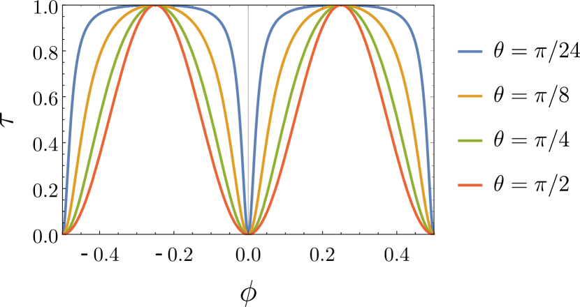
Figure 3: Sharp antiresonances in the normalized conductance $\tau(\phi)$, Eq.  (17), for different values of the magnetic impurity strength.

Fourier spectrum of conductance oscillations is convenient representation for the analysis of experimental data Ziegler et al. (2018); Savchenko et al. (2019). Remarkably, that Fourier coefficients of the transmissions coefficient, $\mathcal{T}^{(n)}=\int d\phi\,\mathcal{T}(\phi)e^{i4\pi\phi n},$ obey universal relation

$$\frac{\mathcal{T}^{(n)}}{\mathcal{T}^{(n+1)}}=-1+2\kappa(\kappa-\sqrt{\kappa^{2}-1})\,,$$ (18)

where $\kappa=\cosh(2\lambda)/\cos\theta$.

An interesting relation between the transmission coefficients $\mathcal{T}_{\alpha}$ can be noticed both in the exact quantum result (16) and in its classical counterpart, (22). While the values of $\mathcal{T}_{\alpha}$ depend on the strength of the magnetic impurity and the flux, one observes that the property

$$\mathcal{T}_{\uparrow}+e^{2\lambda}\mathcal{T}_{\downarrow}=e^{2\lambda}-1,$$

involves only the transparency of the contact, $t=e^{-\lambda}$. It is tempting to regard this property as general one, but further inspection reveals that it holds only for the impurity in the “upper” shoulder of the ring in Fig. 1, while for the impurity in the lower part of the ring we should interchange $\mathcal{T}_{\uparrow}\leftrightarrow\mathcal{T}_{\downarrow}$ in the above formula. For impurities in both shoulders of AB ring the above relation is also violated, which can be checked rather easily for the classical trajectories, using the formulas from Niyazov et al. (2020).

Let us now analyze the limiting cases.

III.1 Open interferometer

For the open interferometer, $\lambda\to\infty$, equations (16) read

$$\mathcal{T} =\frac{1+\cos^{2}\theta}{2}\,,$$ (19)

$$\mathcal{P} =-\frac{\sin^{2}\theta}{2-\sin^{2}\theta}\,.$$

Two possible transmission channels have a trivial contribution to $\mathcal{T}$: spin-down channel conduct electrons without loss, whereas electrons scatter on the magnetic impurity in the spin-up channel with forwarding scattering amplitude $\cos\theta$ (see Fig. 1). For full reflection case, we have $\theta=\pi/2$, $\mathcal{T}=1/2$ and outgoing electrons are fully polarized, $\mathcal{P}=-1$. This is a classical result which is insensitive to dephasing.

III.2 Almost closed interferometer

For the almost closed interferometer, $\lambda\to 0$, the interference contributions play important role:

$$\mathcal{T} =\lambda-\frac{\lambda^{3}\sin^{2}\theta}{1+4\lambda^{2}-\cos^{2}\theta\cos^{2}(2\pi\phi)}\,,$$ (20)

$$\mathcal{P} =-\frac{\lambda\sin^{2}\theta}{1+\lambda^{2}(4-\sin^{2}\theta)-\cos^{2}\theta\cos^{2}(2\pi\phi)}\,.$$

We see that sharp antiresonances appear at half-integer and integer values of the flux, $\phi$ by contrast to conventional interferometers, where only half-integer resonances exist Dmitriev et al. (2015). The difference is related to the absence of backscattering by non-magnetic contacts in the case of helical edge states Niyazov et al. (2018).

III.3 Weak magnetic impurity

For the previously studied case Niyazov et al. (2018, 2020) of weak scattering on the magnetic impurity, $\theta\to 0$, we obtain

$$\mathcal{T} =\tanh\lambda\left(1-\frac{2\theta^{2}\cosh(2\lambda)\sinh^{2}\lambda}{\cosh(4\lambda)-\cos(4\pi\phi)}\right)\,,$$ (21)

$$\mathcal{P} =-\frac{\theta^{2}}{2}\frac{\sinh(4\lambda)}{\cosh(4\lambda)-\cos(4\pi\phi)}\,.$$

IV Quantum flux-independent processes

Let us now discuss one interesting aspect of our central result (16), namely, the possible recovery of the classical contribution upon the averaging over the magnetic flux. Previously we have shown  Niyazov et al. (2018, 2020) that the classical result was correctly reproduced by such averaging when keeping the terms of order $\theta^{2}$. The exact expressions for the classical result was found there as

$$\mathcal{T}_{\text{cl}} =\tanh\lambda\left(1-\frac{1}{2}\frac{\tanh^{2}\lambda\tan^{2}\theta}{1+\tan^{2}\theta\coth(2\lambda)}\right)\,,$$ (22)

$$\mathcal{T}_{s,\text{cl}} =-\frac{1}{2}\frac{\tanh^{2}\lambda\tan^{2}\theta}{1+\tan^{2}\theta\coth(2\lambda)}\,.$$

Now we perform the averaging over the magnetic flux of our quantum result (16) and obtain

$$\langle\mathcal{T}\rangle_{\phi} =\tanh\lambda\left(1-\frac{\sqrt{2}\sin^{2}\theta\sinh^{2}\lambda}{\sqrt{\cosh(4\lambda)-\cos(2\theta)}}\right)\,,$$ (23)

$$\langle\mathcal{T}_{s}\rangle_{\phi} =-\frac{\sqrt{2}\sin^{2}\theta\sinh^{2}\lambda}{\sqrt{\cosh(4\lambda)-\cos(2\theta)}}\,.$$

Clearly these expressions are different and subtracting the purely classical result from the quantum one, averaged over the magnetic flux, we get the non-zero result. It implies the existence of quantum flux-independent processes. They appear first in the order $\theta^{4}$:

$$\mathcal{T}_{\text{cl}}-\langle\mathcal{T}\rangle_{\phi}=-\frac{t^{8}}{\left(1+t^{2}\right)^{4}}\theta^{4}+\mathcal{O}(\theta^{6})\,.$$ (24)

The coefficient $t^{8}$ before $\theta^{4}$ means that the electron is passing the contacts at least four times. The simplest examples of such processes are shown in Fig. 4: panel (a) for spin up $\sim t^{8}+\mathcal{O}(t^{10})$ and panel (b) for spin down $\sim t^{12}+\mathcal{O}(t^{12})$.

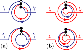
Figure 4: Simplest quantum processes which do not sensitive to magnetic flux.

V Conclusions

We have studied high-temperature transport through the helical Aharonov-Bohm interferometer tunnel-coupled to metallic leads. We focused on effect induced by strong magnetic impurity placed in one arm of the interferometer and demonstrated that the tunneling conductance and the spin polarization of the outgoing electrons show sharp antiresonances at integer and half-integer values of the dimensionless flux $\phi$. We calculated the spin-dependent transmission coefficients, $\mathcal{T}_{\alpha}$, for arbitrary values of the tunneling coupling and the magnetic impurity strength. We generalize previously obtained results, describing transport near the resonant values of $\phi$, to the arbitrary value of magnetic flux. We also discussed special quantum effects which do not show up for weak impurity.

We found optimal conditions for spin filtering. Specifically, we demonstrated that spin polarization of the outgoing electrons reach 100% in the limit of strong magnetic impurity and open interferometer. The conductance of the setup equals in this case $e^{2}/h.$ In this limit all quantum effects are suppressed and the transmission through the interferometer has purely classical nature, i.e. is robust to dephasing.

To conclude, a helical AB interferometer with strong magnetic impurity allows to create large spin polarization. Remarkably, such polarization can be reached even for $\phi=0,$ i.e. without a magnetic field. The scattering strength can be controlled by in-plane magnetic field or by external ferromagnetic tip, providing additional ways to manipulate spin polarization. These features add up to the remarkable properties of topological materials, making them even more attractive for spintronics, magnetic field detection, quantum networking, and quantum computing.

VI Acknowledgements

The calculation of spin polarization (R.N.) was funded by RFBR, project number 19-32-60077. The calculation of conductance (D.A. and V.K.) was funded by the Russian Science Foundation, Grant No. 20-12-00147. The work of R.N. and V.K. was partially supported by Foundation for the Advancement of Theoretical Physics and Mathematics.

References

- Bernevig and Hughes (2013) B. Bernevig and T. Hughes, Topological Insulators and Topological Superconductors (Princeton University Press, 2013).
- Hasan and Kane (2010) M. Z. Hasan and C. L. Kane, Rev. Mod. Phys. 82, 3045 (2010).
- Qi and Zhang (2011) X.-L. Qi and S.-C. Zhang, Rev. Mod. Phys. 83, 1057 (2011).
- Kane and Mele (2005) C. L. Kane and E. J. Mele, Phys. Rev. Lett. 95, 226801 (2005).
- Bernevig et al. (2006) B. A. Bernevig, T. L. Hughes, and S.-C. Zhang, Science 314, 1757 (2006).
- König et al. (2007) M. König, S. Wiedmann, C. Brune, A. Roth, H. Buhmann, L. W. Molenkamp, X.-L. Qi, and S.-C. Zhang, Science 318, 766 (2007).
- Roth et al. (2009) A. Roth, C. Brüne, H. Buhmann, L. W. Molenkamp, J. Maciejko, X.-L. Qi, and S.-C. Zhang, Science 325, 294 (2009).
- Gusev et al. (2011) G. M. Gusev, Z. D. Kvon, O. A. Shegai, N. N. Mikhailov, S. A. Dvoretsky, and J. C. Portal, Phys. Rev. B 84, 121302 (2011).
- Brüne et al. (2012) C. Brüne, A. Roth, H. Buhmann, E. M. Hankiewicz, L. W. Molenkamp, J. Maciejko, X.-L. Qi, and S.-C. Zhang, Nature Physics 8, 485 (2012).
- Kononov et al. (2015) A. Kononov, S. V. Egorov, Z. D. Kvon, N. N. Mikhailov, S. A. Dvoretsky, and E. V. Deviatov, JETP Letters 101, 814 (2015).
- Peng et al. (2010) H. Peng, K. Lai, D. Kong, S. Meister, Y. Chen, X.-L. Qi, S.-C. Zhang, Z.-X. Shen, and Y. Cui, Nat Mater 9, 225 (2010).
- Lin et al. (2017) B.-C. Lin, S. Wang, L.-X. Wang, C.-Z. Li, J.-G. Li, D. Yu, and Z.-M. Liao, Phys. Rev. B 95, 235436 (2017).
- Bardarson et al. (2010) J. H. Bardarson, P. W. Brouwer, and J. E. Moore, Phys. Rev. Lett. 105, 156803 (2010).
- Bardarson and Moore (2013) J. H. Bardarson and J. E. Moore, Reports on Progress in Physics 76, 056501 (2013).
- Delplace et al. (2012) P. Delplace, J. Li, and M. Büttiker, Phys. Rev. Lett. 109, 246803 (2012).
- Gusev et al. (2015) G. Gusev, Z. Kvon, O. Shegai, N. Mikhailov, and S. Dvoretsky, Solid State Communications 205, 4 (2015).
- Chu et al. (2009) R.-L. Chu, J. Li, J. K. Jain, and S.-Q. Shen, Phys. Rev. B 80, 081102 (2009).
- Masuda and Kuramoto (2012) S. Masuda and Y. Kuramoto, Phys. Rev. B 85, 195327 (2012).
- Dutta et al. (2016) P. Dutta, A. Saha, and A. M. Jayannavar, Physical Review B 94, 195414 (2016).
- Konig et al. (2007) M. Konig, S. Wiedmann, C. Brune, A. Roth, H. Buhmann, L. W. Molenkamp, X.-L. Qi, and S.-C. Zhang, Science 318, 766 (2007).
- Knez et al. (2011) I. Knez, R.-R. Du, and G. Sullivan, Phys. Rev. Lett. 107, 136603 (2011).
- Wu et al. (2018) S. Wu, V. Fatemi, Q. D. Gibson, K. Watanabe, T. Taniguchi, R. J. Cava, and P. Jarillo-Herrero, Science 359, 76 (2018).
- Reis et al. (2017) F. Reis, G. Li, L. Dudy, M. Bauernfeind, S. Glass, W. Hanke, R. Thomale, J. Schäfer, and R. Claessen, Science 357, 287 (2017).
- Li et al. (2018) G. Li, W. Hanke, E. M. Hankiewicz, F. Reis, J. Schäfer, R. Claessen, C. Wu, and R. Thomale, Phys. Rev. B 98, 165146 (2018).
- Stühler et al. (2020) R. Stühler, F. Reis, T. Müller, T. Helbig, T. Schwemmer, R. Thomale, J. Schäfer, and R. Claessen, Nat. Phys. 16, 47 (2020).
- Jagla and Balseiro (1993) E. A. Jagla and C. A. Balseiro, Phys. Rev. Lett. 70, 639 (1993).
- Dmitriev et al. (2010) A. P. Dmitriev, I. V. Gornyi, V. Y. Kachorovskii, and D. G. Polyakov, Phys. Rev. Lett. 105, 036402 (2010).
- Shmakov et al. (2013) P. M. Shmakov, A. P. Dmitriev, and V. Y. Kachorovskii, Phys. Rev. B 87, 235417 (2013).
- Dmitriev et al. (2015) A. P. Dmitriev, I. V. Gornyi, V. Y. Kachorovskii, D. G. Polyakov, and P. M. Shmakov, JETP Letters 100, 839 (2015).
- Dmitriev et al. (2017) A. P. Dmitriev, I. V. Gornyi, V. Y. Kachorovskii, and D. G. Polyakov, Phys. Rev. B 96, 115417 (2017).
- Niyazov et al. (2018) R. A. Niyazov, D. N. Aristov, and V. Y. Kachorovskii, Phys. Rev. B 98, 045418 (2018).
- Niyazov et al. (2020) R. A. Niyazov, D. N. Aristov, and V. Y. Kachorovskii, npj Comput. Mater. 6, 174 (2020).
- Du et al. (2015) L. Du, I. Knez, G. Sullivan, and R.-R. Du, Phys. Rev. Lett. 114, 096802 (2015).
- Zhang et al. (2014) S.-B. Zhang, Y.-Y. Zhang, and S.-Q. Shen, Phys. Rev. B 90, 115305 (2014).
- Hu et al. (2016) L.-H. Hu, D.-H. Xu, F.-C. Zhang, and Y. Zhou, Phys. Rev. B 94, 085306 (2016).
- Kurilovich et al. (2017) P. D. Kurilovich, V. D. Kurilovich, I. S. Burmistrov, and M. Goldstein, JETP Lett. 106, 593 (2017).
- Ziegler et al. (2018) J. Ziegler, R. Kozlovsky, C. Gorini, M.-H. Liu, S. Weishäupl, H. Maier, R. Fischer, D. A. Kozlov, Z. D. Kvon, N. Mikhailov, S. A. Dvoretsky, K. Richter, and D. Weiss, Phys. Rev. B 97, 035157 (2018).
- Savchenko et al. (2019) M. L. Savchenko, D. A. Kozlov, N. N. Vasilev, Z. D. Kvon, N. N. Mikhailov, S. A. Dvoretsky, and A. V. Kolesnikov, Phys. Rev. B 99, 195423 (2019).