Machine learning time-local generators of open quantum dynamics
Abstract
In the study of closed many-body quantum systems one is often interested in the evolution of a subset of degrees of freedom. On many occasions it is possible to approach the problem by performing an appropriate decomposition into a bath and a system. In the simplest case the evolution of the reduced state of the system is governed by a quantum master equation with a time-independent, i.e. Markovian, generator. Such evolution is typically emerging under the assumption of a weak coupling between the system and an infinitely large bath. Here, we are interested in understanding to which extent a neural network function approximator can predict open quantum dynamics — described by time-local generators — from an underlying unitary dynamics. We investigate this question using a class of spin models, which is inspired by recent experimental setups. We find that indeed time-local generators can be learned. In certain situations they are even time-independent and allow to extrapolate the dynamics to unseen times. This might be useful for situations in which experiments or numerical simulations do not allow to capture long-time dynamics and for exploring thermalization occurring in closed quantum systems.
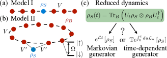
Introduction—The investigation of isolated quantum systems out of equilibrium is a central problem in physics D’Alessio et al. (2016); Polkovnikov et al. (2011). Often, partial information that concerns a spatially localized subsystem is sufficient to study dynamical effects related to relaxation or thermalization. This information is encoded in the so-called reduced quantum state , [c.f. Fig. 1(a,b)], whose time dependence is obtained by “integrating out” the remainder of the evolving many-body system, which is often referred to as bath [see Fig. 1(c)]. In certain settings, e.g. for systems which are weakly interacting with a large environment Breuer et al. (2002); Gardiner and Zoller (2004), the dynamics of the reduced state is effectively described by a quantum master equation Lindblad (1976); Gorini et al. (1976); Alicki and Lendi (2007). In the simplest manifestation, the dynamics of the reduced quantum state is then governed by a time-independent generator acting only on :
| (1) |
Here, is the unitary evolution operator of the full many-body system, the state is the initial state of the many-body system in product form, and indicates the average over the bath . However, the generator does not need to be time-independent and, in most generic instances Chruściński and Kossakowski (2010), it may depend locally on time, , as sketched in Fig. 1(c).
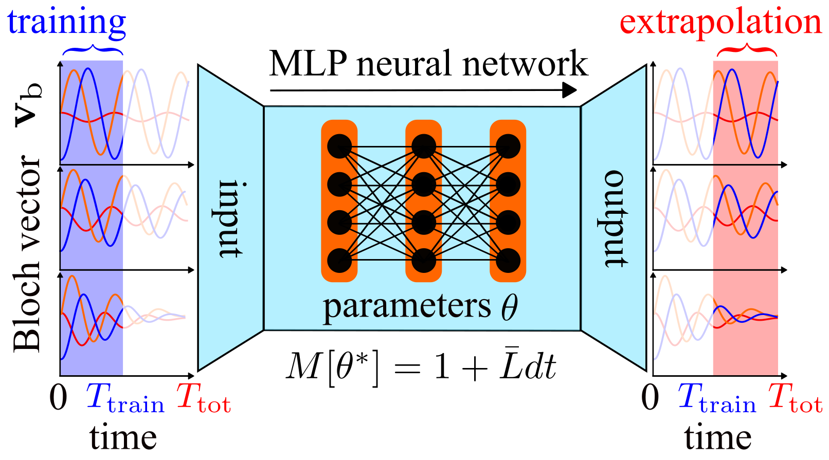
In this paper, we show how simple neural network architectures can learn time-local generators that govern the local dynamics of a closed quantum spin system. The input of the networks consists of the time-dependent average values of the reduced system observables from which the dynamical generator is estimated. Firstly, we consider an architecture which provides a time-averaged generator corresponding to an effectively Markovian description of the system dynamics. Our findings indicate that this can yield indeed a valid approximation for the generator even beyond typical scenarios justifying a Markovian weak-coupling assumption Breuer et al. (2002); Gardiner and Zoller (2004). Once the generator is known, the network can further be exploited to make predictions for times which go beyond the previously analyzed time frame, as is sketched in Fig. 2. To study settings with a time-dependent generator, , we use a different neural network architecture which is based on so-called hypermodels and allows to assess the time-dependence of the generator of the reduced dynamics. Our work links to recent efforts aiming at understanding quantum dynamics with neural networks Yoshioka and Hamazaki (2019); Hartmann and Carleo (2019a); Nagy and Savona (2019); Krastanov et al. (2020); Carleo et al. (2019); Krastanov et al. (2019); Carleo and Troyer (2017); Hartmann and Carleo (2019b); Liu et al. (2020); Luchnikov et al. (2020); Martina et al. (2021); Miles et al. (2020). Our approach, which uses machine learning tools and provides a directly interpretable object such as the physical generator of the dynamics, highlights a possible route for the application of neural networks in the study of the long-time dynamics of local observables in closed quantum systems. Moreover, it may find applications in the context of quantifying the degree of non-Markovianity in reduced quantum dynamics Chruściński and Kossakowski (2010).
Many-body spin models—For illustrating our ideas, we consider two one-dimensional systems (in the following referred to as Model I and II) consisting of interacting spins, which are inspired by recent state-of-the-art quantum simulator experiments with Rydberg atoms Bloch et al. (2012); Kim et al. (2018); Ebadi et al. (2020); Browaeys and Lahaye (2020); Bloch et al. (2008) or trapped ions Islam et al. (2011); Bohnet et al. (2016); Joshi et al. (2020). Model I has open boundary conditions [see Fig. 1(a)]. It features power-law interactions and is described by the Hamiltonian
| (2) |
Here, is a projector on the “up”-state of the -th spin and are Pauli matrices. The parameter accounts for the interaction range, i.e. the power-law decay of the interaction potential, and controls the overall interaction strength with respect to the strength of a transverse field term. The reduced system , for this model, is the middle spin of the chain, as shown in Fig. 1(a). Model II is a closed spin chain [sketched in Fig. 1(b)], with nearest-neighbor interactions and Hamiltonian
| (3) |
Here, the spin with label is singled out as reference spin (forming the system ) and the interaction strength with its neighbors is given by , while the interaction strength among all other spins is . Moreover, we assume that the strength of the transverse field acting on the reference spin can be controlled. Both models capture a whole variety of different scenarios, including short- and long-range interactions, absence and presence of translational invariance as well as weak and strong coupling between local and bath degrees of freedom. They moreover encompass a number of standard scenarios often explored in quantum many-body physics, such as the so-called PXP-model Sun and Robicheaux (2008); Ates et al. (2012); Turner et al. (2018), the Ising model in the presence of longitudinal and transverse fields, and all-to-all connected spin systems with resemblance to the Dicke model Emary and Brandes (2003) or the Lipkin-Meshkov-Glick model Dusuel and Vidal (2004).
Our aim is to investigate the reduced dynamics of local degrees of freedom, as for instance a single spin , as depicted in Fig. 1(a,b). To this end, we assume that the system is initialized at time in the state . In our studies concerning Model I, we assume the bath to be in the infinite temperature state, . When considering Model II, instead, we assume a finite temperature situation with , where the Hamiltonian is the one of Eq. (3) with , and is the inverse temperature. We let the state evolve according to the unitary dynamics , with from which we obtain the full dynamical information about the subsystem . Throughout we will make use of the Bloch vector representation of the subsystem’s density matrix: with . Here the Bloch vector is given in terms of the expectation with respect to the full quantum state at time , and labels the system spin [see Fig. 1(a,b)].
In the following, we will characterize the generator of this reduced dynamics; that is, we want to find a generator acting solely on that reproduces (or approximates) the dynamics of for the two models under consideration [Fig. 1(a,b)]. For Model I we explore for which parameter combinations , the local generator, which is in principle time-dependent , can be approximated by an effective “averaged” time-independent one, . We remark here that, while acts as a fictitious bath for subsystem , the situation described here is far from that of typical weak-coupling limits. Indeed, is a finite quantum system and its Hamiltonian has a discrete spectrum. As such, can hardly be thought of as an infinite Markovian bath of bosonic oscillators, whose state is unaffected by the interaction with . The only aspect in common with a weak-coupling limit is that the interaction strength can be made small. However, this is not sufficient to argue that the local dynamics may be described by time-independent generators.
For Model II we consider the case in which an “isolated” spin (on site ) interacts with with an independently tunable strength . Experimentally such a situation can be realized, e.g., by exploiting the distance dependence of dipolar interactions of atoms in Rydberg states Browaeys and Lahaye (2020). Also for Model II we investigate how well the generator of the reduced dynamics is approximated by a time-independent model when the initial state of (parametrized by the inverse temperature ) and the interaction strength is varied. In addition, for this scenario, we use a hypermodel in order to analyze regimes that necessitate a time-dependent generator .
Network architectures and training—In order to learn dynamical generators for the reduced dynamics of subsystem , we employ machine learning algorithms. Our approach is completely data-driven, i.e. the network has no prior information about the physical system. For learning time-independent generators, we use a linear multi-layer perceptron (MLP) architecture (see Fig. 2) which turns out to be the simplest possible one. Every data-point of our data-set contains the triple where is the value of the Bloch vector at a given time-point , and is the value of the Bloch vector after a further discrete time step , i.e. .
The input of our model is , and the output is the vector , where is a -matrix (matching the dimension of the Bloch vector), that depends on the parameters of the network. To optimize the network, we introduce the following loss function, which is given by the norm of the difference between the next time step and the output of the network:
| (4) |
where the expectation is taken over the training data . Minimizing the above function thus provides a model for the propagation of the Bloch vector over an infinitesimal time step . This model is related to the generator of the local dynamics: indeed, we have , where is a representation of the time-averaged generator acting on Bloch vectors. The training data-set is constructed by evolving the Bloch vector over a time interval . The trajectories are generated evolving randomly chosen initial states of the form
| (5) |
with , i.e. we consider non-pure initial states. We split our data-set such that we consider the of it for training, i.e. finding the best parameters of our model. The remaining form the validation set to assess the performance of the model built in the training phase.
To encode and quantify the time-dependence of dynamical generators, , we use a different architecture and consider a so-called hypermodel, which computes network weights based on a context input. In our case, the context input is the time and a multi-layer perceptron (MLP) with non-linear activation functions transforms this input to the matrix of the generator .
The data-set is organized in the same way as for the time-independent model. The only difference with respect to the previous case is that we also pass the information about the actual time step . The network parameters are optimized by minimizing the loss function
| (6) |
By training the model in this way we obtain a time-dependent representation of the propagator of the local dynamics, i.e. . For the training set, we choose quantum states as in the previous case. For the evaluation data-set, instead, we consider
| (7) |
with being a random number, 111See supplemental material for details.
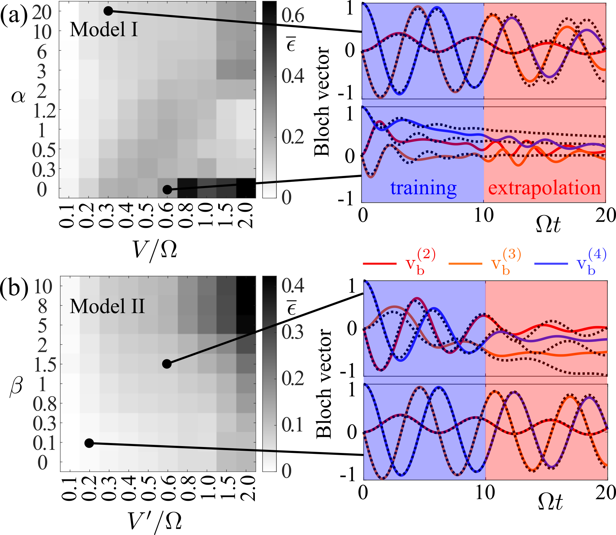
Time-independent generators—With the above numerical approach, we can now investigate under which circumstances the generator of the dynamics of the subsystem is time-independent. We consider first the open spin chain [see Fig. 1(a) and Eq. (2)] and explore different values of and . To test the performance of the model after the training, we study the time-averaged norm difference between the exact Bloch vector — obtained by simulating the full many-body spin chain dynamics — and the time-evolution of the same quantity as predicted by our model :
| (8) |
computed by numerical integration.
As shown in Fig. 3(a), the error is small for short-range (large ) and weakly interacting (with small ratio ) spin chains. This means that our time-independent model captures the relevant features of the reduced dynamics, and suggests that for finite systems with sufficiently weak interactions, the dynamics of local degrees of freedom can indeed be effectively described by a time-independent generator . Furthermore, for this Markovian regime of the dynamics, our model allows to make predictions for times exceeding the training time.
We now turn to the discussion of Model II [see Fig. 1(b) and Eq. (3)]. Using the same procedure explained above, we can learn the time-averaged dynamical generator for subsystem . In Fig. 3(b) we summarize the results of this analysis. We display the time-averaged error, as defined in Eq. (8), for different parameter choices, which in this case are the (inverse) temperature of the initial state and the interaction strength . We furthermore take . As shown in the figure the dynamics is well approximated by a time-independent generator, , for weak interactions and for small . Here also the extrapolation to times that exceed is possible. The data in Fig. 3 shows that in certain parameter regimes the approximation of the dynamics through a time-independent generator does not work well. Here significant deviations are even observable during the training period.
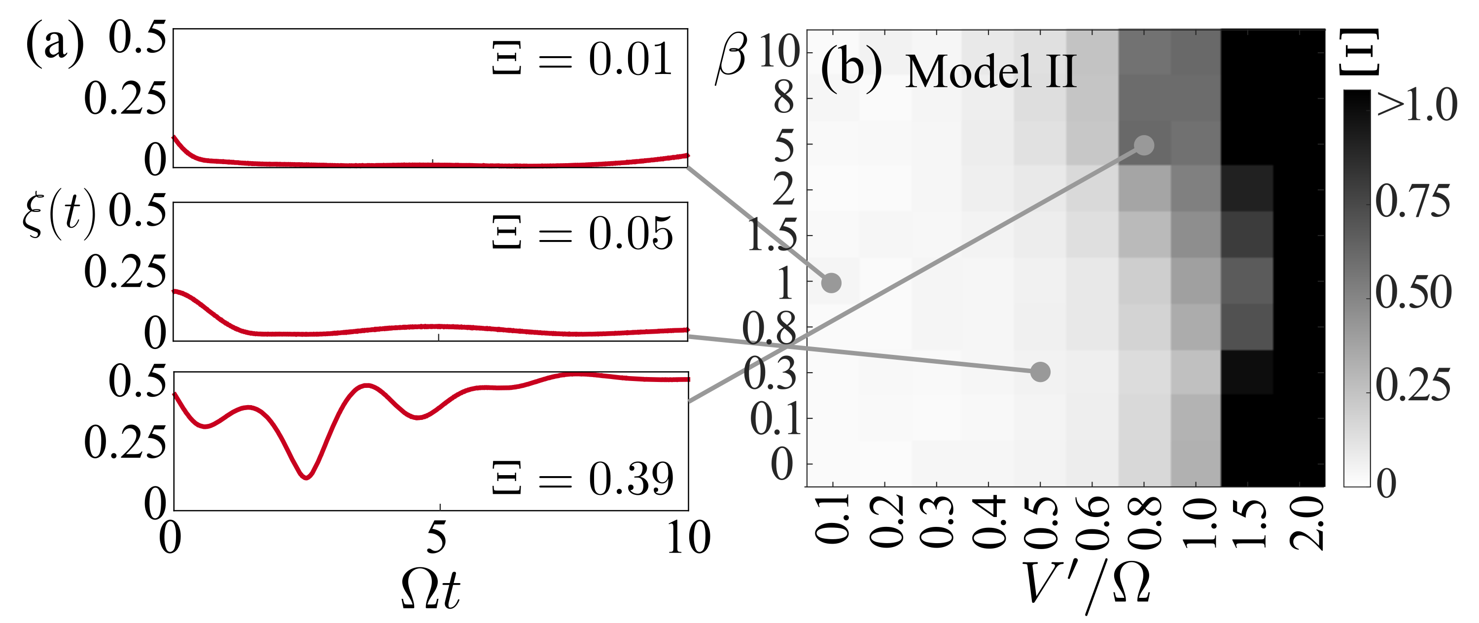
Time-dependent time-local generators—We are now interested in analyzing how strongly the dynamical generator depends on time, in those instances where the model introduced in the previous section fails. To this end, we adopt a hypermodel which can take as input the information about the running time. In this way, the neural network is able to learn an optimal parametrization of the “propagator” for the Bloch vector dynamics which explicitly depends on time. Here, the matrix encodes the action of the generator on the Bloch vector and, essentially, implements the differential equations obeyed by the entries of the Bloch vector . This architecture allows to learn and accurately reproduce the dynamics of Model II for all studied parameter regimes (see Supplemental Material for examples). This is not surprising, but gives us a handle for analyzing the time-dependence of the dynamical generator . To this end we consider the positive quantity , where the dot denotes the derivative with respect to time. This can only be zero when , i.e. when the action of the generator is not depending on the running time. To quantify an overall time-dependence within a time window , we define the time-averaged value . In Fig. 4 we show the corresponding data. For strong interactions , is non-zero throughout which indicates a strong explicit time-dependence. This is also reflected in a large . For weak interactions, on the other hand, remains small for all times considered. The oscillation we attribute to the finite size of the system. This confirms that, in such parameter regime, it is indeed possible to approximate the dynamics of the Bloch vector by means of a time-independent matrix, as considered in the previous section.
Conclusions—We have presented two simple examples of neural network architectures that can learn the dynamical features of reduced quantum states. When such time evolution is effectively Markovian, the network can find a suitable approximation for the generator of the local dynamics. Here one can extrapolate the dynamics of reduced degrees of freedom to times that were unexplored during the training procedure. This possibility is particularly promising for applications in combination with tensor networks, which perform extremely well for short times. A neural network could learn the time-independent generator during this time interval and then possibly extrapolate to long times. In principle, this might enable the exploration of the onset of stationary or thermalization regimes. When the dynamics is not of Markovian type, we have shown that hypermodels can recover the generator of the reduced quantum dynamics. This allows to quantify non-Markovian effects Benatti et al. (2016), which manifest in an explicit time-dependence of the dynamical generator Ref. Chruściński and Kossakowski (2010). Furthermore, being able to reconstruct the generator of the reduced dynamics, as we have done here with hypermodels, makes it possible to explore different measures of non-Markovianity based on non-divisibility criteria for quantum dynamical time-evolutions Breuer et al. (2009); Laine et al. (2010); Breuer (2012); Rivas et al. (2014).
A possible future development in this regard could be the application of more advanced machine learning methods for learning time correlations in time series. This can be achieved with models borrowed from language studies (e.g. long-short term memory recurrent neural networks (LSTM) Hochreiter and Schmidhuber (1997) and transformers Vaswani et al. (2017)) or with algorithms geared towards more interpretable models by either learning analytical expressions of the differential equation Sahoo et al. (2018) or by modelling the time-evolution dynamics directly Chen et al. (2018).
Acknowledgements.
Acknowledgments—We acknowledge financial support from the Deutsche Forschungsgemeinschaft (DFG, German Research Foundation) under Germany’s Excellence Strategy – EXC-Number 2064/1 – Project number 390727645. IL acknowledges funding from the “Wissenschaftler Rückkehrprogramm GSO/CZS” of the Carl-Zeiss-Stiftung and the German Scholars Organization e.V., and through the DFG projects number 428276754 (SPP GiRyd) and 435696605. The authors thank the International Max Planck Research School for Intelligent Systems (IMPRS-IS) for supporting DZ.References
- D’Alessio et al. (2016) L. D’Alessio, Y. Kafri, A. Polkovnikov, and M. Rigol, Adv. Phys. 65, 239 (2016).
- Polkovnikov et al. (2011) A. Polkovnikov, K. Sengupta, A. Silva, and M. Vengalattore, Rev. Mod. Phys. 83, 863 (2011).
- Breuer et al. (2002) H.-P. Breuer, F. Petruccione, et al., The theory of open quantum systems (Oxford University Press on Demand, 2002).
- Gardiner and Zoller (2004) C. Gardiner and P. Zoller, Quantum noise: a handbook of Markovian and non-Markovian quantum stochastic methods with applications to quantum optics (Springer Science & Business Media, 2004).
- Lindblad (1976) G. Lindblad, Commun. Math. Phys. 48, 119 (1976).
- Gorini et al. (1976) V. Gorini, A. Kossakowski, and E. C. G. Sudarshan, Journal of Mathematical Physics 17, 821 (1976).
- Alicki and Lendi (2007) R. Alicki and K. Lendi, Quantum dynamical semigroups and applications, Vol. 717 (Springer, 2007).
- Chruściński and Kossakowski (2010) D. Chruściński and A. Kossakowski, Phys. Rev. Lett. 104, 070406 (2010).
- Yoshioka and Hamazaki (2019) N. Yoshioka and R. Hamazaki, Phys. Rev. B 99, 214306 (2019).
- Hartmann and Carleo (2019a) M. J. Hartmann and G. Carleo, Phys. Rev. Lett. 122, 250502 (2019a).
- Nagy and Savona (2019) A. Nagy and V. Savona, Phys. Rev. Lett. 122, 250501 (2019).
- Krastanov et al. (2020) S. Krastanov, K. Head-Marsden, S. Zhou, S. T. Flammia, L. Jiang, and P. Narang, arXiv:2009.03902 (2020).
- Carleo et al. (2019) G. Carleo, I. Cirac, K. Cranmer, L. Daudet, M. Schuld, N. Tishby, L. Vogt-Maranto, and L. Zdeborová, Rev. Mod. Phys. 91, 045002 (2019).
- Krastanov et al. (2019) S. Krastanov, S. Zhou, S. T. Flammia, and L. Jiang, Quantum Sci. Technol. 4, 035003 (2019).
- Carleo and Troyer (2017) G. Carleo and M. Troyer, Science 355, 602 (2017).
- Hartmann and Carleo (2019b) M. J. Hartmann and G. Carleo, Phys. Rev. Lett. 122, 250502 (2019b).
- Liu et al. (2020) Z. Liu, L.-M. Duan, and D.-L. Deng, arXiv:2008.05488 (2020).
- Luchnikov et al. (2020) I. A. Luchnikov, S. V. Vintskevich, D. A. Grigoriev, and S. N. Filippov, Phys. Rev. Lett. 124, 140502 (2020).
- Martina et al. (2021) S. Martina, S. Gherardini, and F. Caruso, arXiv:2101.03221 (2021).
- Miles et al. (2020) C. Miles, A. Bohrdt, R. Wu, C. Chiu, M. Xu, G. Ji, M. Greiner, K. Q. Weinberger, E. Demler, and E.-A. Kim, arXiv:2011.03474 (2020).
- Bloch et al. (2012) I. Bloch, J. Dalibard, and S. Nascimbène, Nat. Phys. 8, 267 (2012).
- Kim et al. (2018) H. Kim, Y. Park, K. Kim, H.-S. Sim, and J. Ahn, Phys. Rev. Lett. 120, 180502 (2018).
- Ebadi et al. (2020) S. Ebadi, T. T. Wang, H. Levine, A. Keesling, G. Semeghini, A. Omran, D. Bluvstein, R. Samajdar, H. Pichler, W. W. Ho, et al., arXiv:2012.12281 (2020).
- Browaeys and Lahaye (2020) A. Browaeys and T. Lahaye, Nat. Phys. 16, 132–142 (2020).
- Bloch et al. (2008) I. Bloch, J. Dalibard, and W. Zwerger, Rev. Mod. Phys. 80, 885 (2008).
- Islam et al. (2011) R. Islam, E. Edwards, K. Kim, S. Korenblit, C. Noh, H. Carmichael, G.-D. Lin, L.-M. Duan, C.-C. J. Wang, J. Freericks, et al., Nat. Comm. 2, 1 (2011).
- Bohnet et al. (2016) J. G. Bohnet, B. C. Sawyer, J. W. Britton, M. L. Wall, A. M. Rey, M. Foss-Feig, and J. J. Bollinger, Science 352, 1297 (2016).
- Joshi et al. (2020) M. K. Joshi, A. Elben, B. Vermersch, T. Brydges, C. Maier, P. Zoller, R. Blatt, and C. F. Roos, Phys. Rev. Lett. 124, 240505 (2020).
- Sun and Robicheaux (2008) B. Sun and F. Robicheaux, New J. Phys. 10, 045032 (2008).
- Ates et al. (2012) C. Ates, J. P. Garrahan, and I. Lesanovsky, Phys. Rev. Lett. 108, 110603 (2012).
- Turner et al. (2018) C. Turner, A. Michailidis, D. Abanin, M. Serbyn, and Z. Papić, Nat. Phys. 14, 745 (2018).
- Emary and Brandes (2003) C. Emary and T. Brandes, Phys. Rev. E 67, 066203 (2003).
- Dusuel and Vidal (2004) S. Dusuel and J. Vidal, Phys. Rev. Lett. 93, 237204 (2004).
- Note (1) See supplemental material for details.
- Benatti et al. (2016) F. Benatti, F. Carollo, R. Floreanini, and H. Narnhofer, Phys. Lett. A 380, 381 (2016).
- Breuer et al. (2009) H.-P. Breuer, E.-M. Laine, and J. Piilo, Phys. Rev. Lett. 103, 210401 (2009).
- Laine et al. (2010) E.-M. Laine, J. Piilo, and H.-P. Breuer, Phys. Rev. A 81, 062115 (2010).
- Breuer (2012) H.-P. Breuer, J. Phys. B 45, 154001 (2012).
- Rivas et al. (2014) Á. Rivas, S. F. Huelga, and M. B. Plenio, Rep. Prog. Phys. 77, 094001 (2014).
- Hochreiter and Schmidhuber (1997) S. Hochreiter and J. Schmidhuber, Neural Comput. 9, 1735 (1997).
- Vaswani et al. (2017) A. Vaswani, N. Shazeer, N. Parmar, J. Uszkoreit, L. Jones, A. N. Gomez, L. Kaiser, and I. Polosukhin, arXiv:1706.03762 (2017).
- Sahoo et al. (2018) S. S. Sahoo, C. H. Lampert, and G. Martius, in Proc. 35th International Conference on Machine Learning, ICML 2018, Stockholm, Sweden, 2018, Vol. 80 (PMLR, 2018) pp. 4442–4450.
- Chen et al. (2018) R. T. Q. Chen, Y. Rubanova, J. Bettencourt, and D. K. Duvenaud, in Advances in Neural Information Processing Systems, Vol. 31, edited by S. Bengio, H. Wallach, H. Larochelle, K. Grauman, N. Cesa-Bianchi, and R. Garnett (Curran Associates, Inc., 2018) pp. 6571–6583.
Supplemental material: Machine learning time-local generators of open quantum dynamics
In this supplemental material we report a more detailed analysis concerning the effectiveness of the hypermodel in predicting the dynamics of the Bloch vector within the training time-window. In addition, we provide the hyper-parameters of the used models.
I Hypermodel vs. exact dynamics
In the main text we analyze the time-dependence of time-local generators parametrizing the “propagator” for the Bloch vector, using a hypermodel architecture. The matrix encodes all the information concerning the dynamics of local (one-site) observables. As stated in the main text, a suitable measure to quantify the dependence on time of this matrix is given by , where . However, this can be a faithful measure of the time-dependence of the physical generator, only if correctly implements the dynamics of the Bloch vector. It is thus important to check that the prediction of the hypermodel matches the exact dynamics, in the time window in which we want to analyze the generator . To this end, we report in Fig. 1 a detailed comparison between the predicted time evolution of the Bloch vector components and the exact ones for six different parameter regimes.
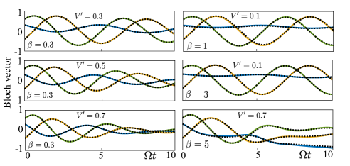
We start from a generic initial state of the form
| (1) |
with , in particular we choose , and , and we consider different interactions and initial bath temperatures. In the training time-window , we observe an excellent agreement between the two curves for . In Fig. 2 we report the time evolution of the quantity for the same parameter regimes.
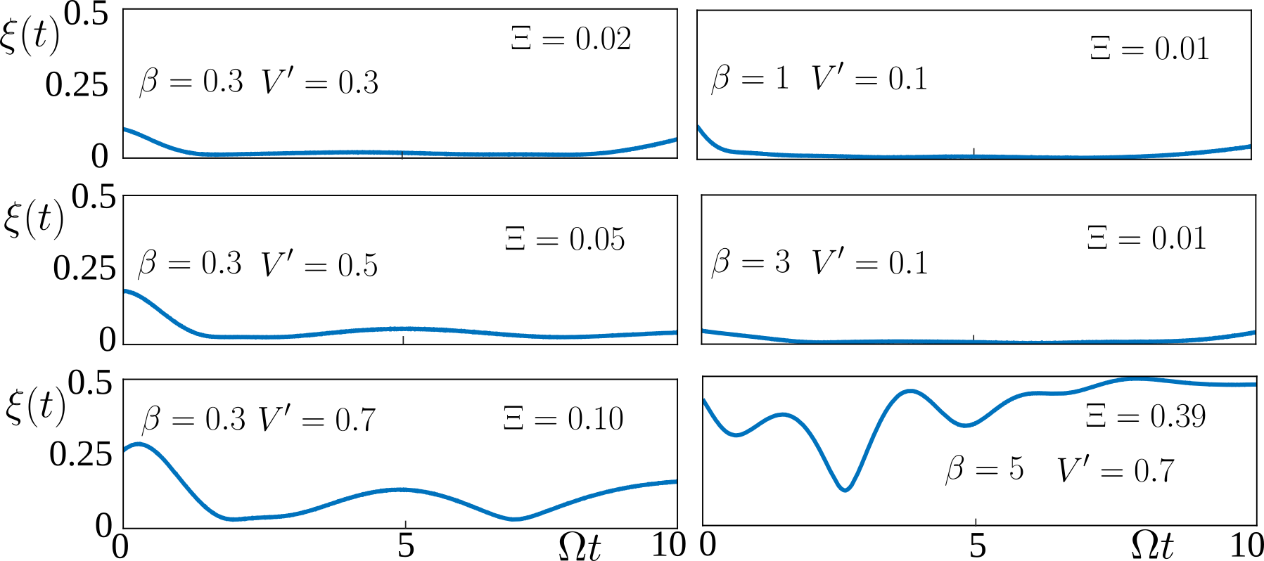
As it can be observed for weakly interacting systems the generator is almost time-independent. In this regime, as discussed in the main text, it is possible to predict the local dynamics using simple time-independent architectures. Increasing the interaction, the parameter grows accordingly signaling that the dependence on time of becomes stronger.
The training procedure for the hyper-model is slightly different with respect what we have done for the time-independent case, in particular it is different the differentiation between training and evaluation set. In this case, in fact, we generate two different types of data-sets, the first data-set for training consists in trajectories with randomly chosen initial state of the the same form reported in Eq. (1). For evaluation we select, instead, randomly data-points from trajectories generated from initial states of type
| (2) |
with . In this way we are performing a separation of the data-sets in the Hilbert space. This is contrary to what we had for the time-independent case where the data-set was given by separated time-intervals of the same trajectory.
II Network architectures
| Setting | Architecture | Optimizer | Dataset |
| Time-independent | Linear perceptron (no hidden layers) | Adam Learning rate: Betas: , Epsilon: Batch size: Batches per epoch: Epochs: | Trajectories (train / val): / Total time (): Time step (): |
| Time-dependent (hyper-model) | Hidden layers: Nonlinearity: tanh Output nonlinearity: none | Adam Learning rate: Betas: , Epsilon: Batch size: Batches per epoch: Epochs: | Trajectories (train / val): / Total time (): Time step (): |