Univariate polynomials and the contractibility of certain sets

Abstract.

We consider the set $\Pi^{*}_{d}$ of monic polynomials $Q_{d}=x^{d}+\sum_{j=0}^{d-1}a_{j}x^{j}$, $x\in\mathbb{R}$, $a_{j}\in\mathbb{R}^{*}$, having $d$ distinct real roots, and its subsets defined by fixing the signs of the coefficients $a_{j}$. We show that for every choice of these signs, the corresponding subset is non-empty and contractible. A similar result holds true in the cases of polynomials $Q_{d}$ of even degree $d$ and having no real roots or of odd degree and having exactly one real root. For even $d$ and when $Q_{d}$ has exactly two real roots which are of opposite signs, the subset is contractible. For even $d$ and when $Q_{d}$ has two positive (resp. two negative) roots, the subset is contractible or empty. It is empty exactly when the constant term is positive, among the other even coefficients there is at least one which is negative, and all odd coefficients are positive (resp. negative).

Key words: real polynomial in one variable; hyperbolic polynomial; Descartes’ rule of signs

AMS classification: 26C10; 30C15

1. Introduction

In the present paper we consider the general family of real monic univariate polynomials $Q_{d}=x^{d}+\sum_{j=0}^{d-1}a_{j}x^{j}$. It is a classical fact that the subsets of $\mathbb{R}^{d}\cong Oa_{0}\ldots a_{d-1}$ of values of the coefficients $a_{j}$ for which the polynomial $Q_{d}$ has one and the same number of distinct real roots are contractible open sets. These sets are the $[d/2]+1$ open parts of $R_{1,d}:=\mathbb{R}^{d}\setminus\Delta_{d}$, where $\Delta_{d}$ is the discriminant set corresponding to the family $Q_{d}$.

Remarks 1.

(1) One defines the discriminant set by the two conditions:

(a) The set $\Delta^{1}_{d}$ is defined by the equality Res$(Q_{d},Q_{d}^{\prime},x)=0$, where Res$(Q_{d},Q_{d}^{\prime}$, $x)$ is the resultant of the polynomials $Q_{d}$ and $Q_{d}^{\prime}$, i. e. the determinant of the corresponding Sylvester matrix.

(b) One sets $\Delta_{d}:=\Delta^{1}_{d}\setminus\Delta^{2}_{d}$, where $\Delta^{2}_{d}$ is the set of values of the coefficients $a_{j}$ for which there is a multiple complex conjugate pair of roots of $Q_{d}$ and no multiple real root.

One observes that dim$(\Delta_{d})=$dim$(\Delta^{1}_{d})=d-1$ and dim$(\Delta^{2}_{d})=d-2$. Thus $\Delta_{d}$ is the set of values of $(a_{0},\ldots,a_{d-1})$ for which the polynomial $Q_{d}$ has a multiple real root.

(2) The discriminant set is invariant under the one-parameter group of quasi-homogeneous dilatations $a_{j}\mapsto u^{d-j}a_{j}$, $j=0$, $\ldots,~{}d$.

Remark 1.

If one considers the subsets of $\mathbb{R}^{d}$ for which the polynomial $Q_{d}$ has one and the same numbers of positive and negative roots (all of them distinct) and no zero roots, then these sets will be the open parts of the set $R_{2,d}:=\mathbb{R}^{d}\setminus(\Delta_{d}\cup\{a_{0}=0\})$. To prove their connectedness one can consider the mapping “roots $\mapsto$ coefficients”. Given two sets of nonzero roots with the same numbers of negative and positive roots (in both cases they are all simple) one can continuously deform the first set into the second one while keeping the absence of zero roots, the numbers of positive and negative roots and their simplicity throughout the deformation. The existence of this deformation implies the existence of a continuous path in the set $R_{2,d}$ connecting the two polynomials $Q_{d}$ with the two sets of roots.

In the present text we focus on polynomials without vanishing coefficients and we consider the set

$$R_{3,d}:=\mathbb{R}^{d}\setminus(\Delta_{d}\cup\{a_{0}=0\}\cup\{a_{1}=0\}\cup\cdots\cup\{a_{d-1}=0\})~{}.$$

We discuss the question when its subsets corresponding to given numbers of positive and negative roots of $Q_{d}$ and to given signs of its coefficients are contractible.

Notation 1.

(1) We denote by $\sigma$ the $d$-tuple $($sign$(a_{0}),\ldots$, sign$(a_{d-1}))$, where sign$(a_{j})=+$ or $-$, by $\mathcal{E}_{d}$ the set of elliptic polynomials $Q_{d}$, i. e. polynomials with no real roots (hence $d$ is even and $a_{0}>0$), and by $\mathcal{E}_{d}(\sigma)\subset\mathcal{E}_{d}$ the set consisting of elliptic polynomials $Q_{d}$ with signs of the coefficients defined by $\sigma$.

(2) For $d$ odd and for a given $d$-tuple $\sigma$, we denote by $\mathcal{F}_{d}(\sigma)$ the set of monic real polynomials $Q_{d}$ with signs of their coefficients defined by the $d$-tuple $\sigma$ and having exactly one real (and simple) root.

(3) For $d$ even, we denote by $\mathcal{G}_{d}(\sigma)$ the set of polynomials $Q_{d}$ having signs of the coefficients defined by the $d$-tuple $\sigma$ and having exactly two simple real roots.

Remark 2.

For an elliptic polynomial $Q_{d}$, one has $a_{0}>0$, because for $a_{0}<0$, there is at least one positive root. The sign of the real root of a polynomial of $\mathcal{F}_{d}(\sigma)$ is opposite to sign$(a_{0})$. A polynomial from $\mathcal{G}_{d}(\sigma)$ has two roots of same (resp. of opposite) signs if $a_{0}>0$ (resp. if $a_{0}<0$).

In order to formulate our first result we need the following definition:

Definition 1.

(1) For $d$ even and $a_{0}<0$, we set $\mathcal{G}_{d,(1,1)}(\sigma):=\mathcal{G}_{d}(\sigma)$. For $d$ even and $a_{0}>0$, we set $\mathcal{G}_{d}(\sigma):=\mathcal{G}_{d,(2,0)}(\sigma)\cup\mathcal{G}_{d,(0,2)}(\sigma)$, where for $Q_{d}\in\mathcal{G}_{d,(2,0)}$ (resp. $Q_{d}\in\mathcal{G}_{d,(0,2)}$), $Q_{d}$ has two positive (resp. two negative) distinct roots and no other real roots. Clearly $\mathcal{G}_{d,(2,0)}(\sigma)\cap\mathcal{G}_{d,(0,2)}(\sigma)=\emptyset$.

(2) For $d$ even, we define two special cases according to the signs of the coefficients of $Q_{d}$ and the quantities of its positive or negative real roots:

Case 1). The constant term and all coefficients of monomials of odd degrees are positive, there is at least one coefficient of even degree which is negative, and $Q_{d}$ has $2$ positive and no negative roots.

Case 2). The constant term is positive, all coefficients of monomials of odd degrees are negative, there is at least one coefficient of even degree which is negative, and $Q_{d}$ has $2$ negative and no positive roots.

Cases 1) and 2) are exchanged when one performs the change of variable $x\mapsto-x$.

Our first result concerns real polynomials with not more than $2$ real roots:

Theorem 1.

(1) For $d$ even and for each $d$-tuple $\sigma$, the subset $\mathcal{E}_{d}(\sigma)\subset\mathcal{E}_{d}$ is non-empty and convex hence contractible.

(2) For $d$ odd and for each $d$-tuple $\sigma$, the set $\mathcal{F}_{d}(\sigma)$ is non-empty and contractible.

(3) For $d$ even and for each $d$-tuple $\sigma$ with $a_{0}<0$, the set $\mathcal{G}_{d,(1,1)}(\sigma)$ is contractible. For $d$ even and for each $d$-tuple $\sigma$ with $a_{0}>0$, each set $\mathcal{G}_{d,(2,0)}(\sigma)$ (resp. $\mathcal{G}_{d,(0,2)}(\sigma)$) is contractible or empty. It is empty exactly in Case 1) (resp. in Case 2)).

The theorem is proved in Section 4. The next result of this paper concerns hyperbolic polynomials, i. e. polynomials $Q_{d}$ with $d$ real roots counted with multiplicity.

Notation 2.

We denote by $\Pi_{d}$ the hyperbolicity domain, i. e. the subset of $\mathbb{R}^{d}$ for which the corresponding polynomial $Q_{d}$ is hyperbolic. The interior of $\Pi_{d}$ is the set of polynomials having $d$ distinct real roots and its border $\partial\Pi_{d}$ equals $\Delta_{d}\cap\Pi_{d}$. We set

$$\Pi_{d}^{*}:=\Pi_{d}\setminus(\Delta_{d}\cup\{a_{0}=0\}\cup\{a_{1}=0\}\cup\cdots\cup\{a_{d-1}=0\})~{}.$$

Thus $\Pi_{d}^{*}$ is the set of monic degree $d$ univariate polynomials with $d$ distinct real roots and with all coefficients non-vanishing. We denote by $\Pi_{d}^{k}$ and $\Pi_{d}^{*k}$ the projections of the sets $\Pi_{d}$ and $\Pi_{d}^{*}$ in the space $Oa_{d-k}\ldots a_{d-1}$ (hence $\Pi_{d}^{d}=\Pi_{d}$ and $\Pi_{d}^{*d}=\Pi_{d}^{*}$), by $\partial\Pi_{d}^{k}$ the border of $\Pi_{d}^{k}$ and by $pos$ and $neg$ the numbers of positive and negative roots of a polynomial $Q_{d}$ having no vanishing coefficients.

We set $a:=(a_{0},a_{1},\ldots,a_{d-1})$, $a^{\prime}:=(a_{1},\ldots,a_{d-1})$, $a^{\prime\prime}:=(a_{2},\ldots,a_{d-1})$ and $a^{(k)}:=(a_{k},\ldots,a_{d-1})$. In what follows we use the same notation for functions and for their graphs.

Remarks 2.

(1) For a hyperbolic polynomial with no vanishing coefficients, the $d$-tuple $\sigma$ defines the numbers $pos$ and $neg$. Indeed, by Descartes’ rule of signs a real univariate polynomial $Q_{d}$ with $c$ sign changes in its sequence of coefficients has $\leq c$ positive roots and the difference $c-pos$ is even, see [13] and [10]. When applying this rule to the polynomial $Q(-x)$ one finds that the number $p$ of sign preservations is $\geq neg$ and the difference $p-neg$ is even. For a hyperbolic polynomial one has $pos+neg=c+p=d$, so in this case $c=pos$ and $p=neg$.

(2) By Rolle’s theorem the non-constant derivatives of a hyperbolic polynomial (resp. of a polynomial of the set $\Pi_{d}^{*}$) are also hyperbolic (resp. are hyperbolic with all roots non-zero and simple). Hence for two hyperbolic polynomials of the same degree and with the same signs of their respective coefficients, their derivatives of the same orders have one and the same numbers of positive and negative roots.

Our next result is the following theorem (proved in Section 5):

Theorem 2.

For each $d$-tuple $\sigma$, there exists exactly one open component of the set $\Pi_{d}^{*}$ the polynomials $Q_{d}$ from which have exactly $pos$ positive simple and $neg$ negative simple roots and have signs of the coefficients as defined by $\sigma$. This component is contractible.

One can give more explicit information about the components of the set $\Pi_{d}^{*}$. Denote by $M$ such a component defined after a $d$-tuple $\sigma$ and by $M^{k}$ its projection in the space $Oa_{d-k}\cdots a_{d-1}$. It is shown in [19] (see Proposition 1 therein) that $M$ is non-empty. In Section 5 we prove the following statement:

Theorem 3.

For $k\geq 3$, the set $M^{k}$ is the set of all points between the graphs $L^{k}_{\pm}$ of two continuous functions defined on $M^{k-1}$:

$$M^{k}=\{a^{(d-k)}\in\mathbb{R}^{d-k}~{}|~{}L^{k}_{-}(a^{(d-k+1)})<a_{d-k}<L^{k}_{+}(a^{(d-k+1)}),~{}a^{(d-k+1)}\in M^{k-1}\}~{}.$$

The functions $L^{k}_{\pm}$ can be extended to continuous functions defined on $\overline{M^{k-1}}$, whose values might coincide (but this does not necessarily happen) only on $\partial M^{k-1}$.

Remark 3.

Theorem 2 can be deduced from Theorem 3 (but we give in Section 5 a direct proof which is short enough). Indeed, given a component $M$ of the set $\Pi_{d}^{*}$, one can successively contract it into its projections $M^{d-1}$, $M^{d-2}$, $\ldots$, $M^{2}$. The latter is one of the sets $\Pi^{*2}_{d\pm\pm}$ defined in Example 2 which are contractible.

In Section 2 we remind some results which are used in the proof of Theorem 2. In Section 3 we introduce some notation and we give examples concerning the sets $\Pi_{d}$ and $\Pi_{d}^{*}$ for $d=1$, $2$ and $3$. These examples are used in the proofs of Theorems 2 and 3. In Section 6 we make comments on Theorems 1, 2 and 3 and we formulate open problems.

2. Known results about the hyperbolicity domain

Before proving Theorems 1, 2 and 3 we remind some results about the set $\Pi_{d}$ which are due to V. I. Arnold, A. B. Givental and the author, see [3], [11] and [14] or Chapter 2 of [17] and the references therein.

Notation 3.

We denote by $K_{d}$ the simplicial angle $\{x_{1}\geq x_{2}\geq\cdots\geq x_{d}\}\subset\mathbb{R}^{d}$ and by $\tilde{\mathcal{V}}$ the Viète mapping

$$\tilde{\mathcal{V}}:(x_{1},\ldots,x_{d})\mapsto(\varphi_{1},\ldots,\varphi_{d})~{},~{}~{}~{}\,\,\varphi_{j}=\sum_{1\leq i_{1}<i_{2}<\cdots<i_{j}\leq d}x_{i_{1}}x_{i_{2}}\cdots x_{i_{j}}~{}.$$

Strata of $K_{d}$ are denoted by their multiplicity vectors. E. g. for $d=5$, the stratum of $K_{5}$ defined by the multiplicity vector $(2,2,1)$ is the set $\{x_{1}=x_{2}>x_{3}=x_{4}>x_{5}\}\subset\mathbb{R}^{5}$. The same notation is used for strata of $\Pi_{d}$ which is justified by parts (3) and (4) of Theorem 4.

Remark 4.

The set $\Delta_{d}\cap\Pi_{d}=\Delta^{1}_{d}\cap\Pi_{d}$ consists of points $a\in\Pi_{d}\subset\mathbb{R}^{d}$, for which the hyperbolic polynomial $Q_{d}$ has at least one root of multiplicity $\geq 2$. That is why $\Pi_{d}\setminus\Delta_{d}=\Pi_{d}\setminus\Delta^{1}_{d}=S_{1^{d}}$ is the stratum of $\Pi_{d}$ with multiplicity vector $1^{d}=(1,\ldots,1)$ and

$$\Pi_{d}^{*}=S_{1^{d}}\setminus(\{a_{0}=0\}\cup\cdots\cup\{a_{d-1}=0\})~{}.$$

The strata of $\Pi_{d}^{*}$ (they are all of dimension $d$, so they can also be called components) are of the form

$$S_{1^{d}}(\sigma):=\{a\in S_{1^{d}}~{}|~{}{\rm sign}(a_{j})=\sigma_{j},0\leq j\leq d-1\}$$

for some $\sigma=(\sigma_{0},\ldots,\sigma_{d-1})\in\{\pm\}^{d}$.

Theorem 4.

(1) For $k\geq 3$, every non-empty fibre $\tilde{f}_{k}$ of the projection $\pi^{k}:\Pi_{d}^{k}\rightarrow\Pi_{d}^{k-1}$ is either a segment or a point.

(2) The fibre $\tilde{f}_{k}$ is a segment (resp. a point) exactly if the fibre is over a point of the interior of $\Pi_{d}^{k-1}$ (resp. over $\partial\Pi_{d}^{k-1}$).

(3) The mapping $\tilde{\mathcal{V}}:K_{d}\rightarrow\Pi_{d}$ is a homeomorphism.

(4) The restriction of the mapping $\tilde{\mathcal{V}}$ to (the closure of) any stratum of $K_{d}$ defines a homeomorphism of the (closure of the) stratum onto its image which is (the closure of) a stratum of $\Pi_{d}$.

(5) A stratum $S$ of $\Pi_{d}$ defined by a multiplicity vector with $\ell$ components is a smooth $\ell$-dimensional real submanifold in $\mathbb{R}^{d}$. It is the graph of a smooth $(d-\ell)$-dimensional vector-function defined on the projection of the stratum in $Oa_{d-\ell}\ldots a_{d-1}$. Thus $S$ is a real manifold with boundary. The field of tangent spaces to $S$ continuously extends to the strata from the closure of $S$. The extension is everywhere transversal to the space $Oa_{0}\ldots a_{d-\ell-1}$. That is, the sum of the two vector spaces $Oa_{0}\ldots a_{d-\ell-1}$ and (the extension of) the field of tangent spaces to $S$ is the space $Oa_{0}\ldots a_{d-1}$.

(6) For $k\geq 3$, the set $\Pi_{d}^{k}$ is the set of points on and between the graphs $H^{k}_{+}$ and $H^{k}_{-}$ of two locally Lipschitz functions defined on $\Pi_{d}^{k-1}$ whose values coincide on and only on $\partial\Pi_{d}^{k-1}$:

$$\begin{array}[]{ccl}\Pi_{d}^{k}&=&\{(a_{d-k},a^{(d-k+1)})\in\mathbb{R}\times\Pi_{d}^{k-1}~{}|~{}H^{k}_{-}(a^{(d-k+1)})\leq a_{d-k}\leq H^{k}_{+}(a^{(d-k+1)})\}~{},\\ \\ &&$$(H^{k}_{-}(a^{(d-k+1)})=H^{k}_{+}(a^{(d-k+1)}))\Leftrightarrow(a^{(d-k+1)}\in\partial\Pi_{d}^{k-1})~{}.\end{array}$$

(7) For $k\geq 3$, the graph $H^{k}_{+}$ (resp. $H^{k}_{-}$) consists of the closures of the strata whose multiplicity vectors are of the form $(r,1,s,1,\ldots)$ (resp. $(1,r,1,s,\ldots)$) and which have exactly $k-1$ components. (In [17] it is written “$k$ components” which is wrong.)

(8) For $2\leq k\leq\ell$, the projection $S^{k}$ of every $\ell$-dimensional stratum $S$ of $\Pi_{d}$ in the space $Oa_{d-k}\ldots a_{d-1}$ is the set of points on and between the graphs $H^{k}_{+}(S)$ and $H^{k}_{-}(S)$ of two locally Lipschitz functions defined on the closure $\overline{S^{k-1}}$ of $S^{k-1}$ whose values coincide on and only on $\partial S^{k-1}$.

Remarks 3.

(1) The projections $\pi^{k}$ are defined also for $k=2$. For $k=2$, each fibre $\tilde{f}_{2}$ is a half-line and only the graph $H_{2}^{+}$ (but not $H_{2}^{-}$) is defined, see Example 2.

(2) Consider two strata $S_{1}$ and $S_{2}$ of $\Pi_{d}$ defined by their multiplicity vectors $\mu(S_{1})$ and $\mu(S_{2})$. The stratum $S_{2}$ belongs to the topological and algebraic closure of the stratum $S_{1}$ if and only if the vector $\mu(S_{2})$ is obtained from the vector $\mu(S_{1})$ by finitely-many replacings of two consecutive components by their sum.

Remark 5.

For $m\geq 2$, consider the fibres $f^{\diamond}_{m}$ of the projection

$$\pi^{m}_{*}~{}:~{}\Pi_{d}\rightarrow\Pi_{d}^{m}~{}~{}~{}\,,~{}~{}~{}\,\pi^{m}_{*}:=\pi^{m+1}\circ\cdots\circ\pi^{d}~{}.$$

In particular, $\tilde{f}_{d}=f^{\diamond}_{d-1}$. Suppose that such a fibre $f^{\diamond}_{m}$ is over a point $A:=(a_{d-m}^{0},\ldots,a_{d-1}^{0})\in\Pi_{d}^{m}$. When non-empty, the fibre $f^{\diamond}_{m}$ is either a point (when $A\in\partial\Pi_{d}^{m}$) or a set homeomorphic to a $(d-m)$-dimensional cell and its boundary (when $A\in\Pi_{d}^{m}\setminus\partial\Pi_{d}^{m}$). This follows from part (6) of Theorem 4. The boundary of the cell can be represented as consistsing of:

– two $0$-dimensional cells (these are the graphs of the functions $H^{m+1}_{\pm}|_{A}$),

– two $1$-dimensional cells (the graphs of $H^{m+2}_{\pm}|_{(\pi^{m+1})^{-1}(A)}$),

– two $2$-dimensional cells (the graphs of $H^{m+3}_{\pm}|_{(\pi^{m+1}\circ\pi^{m+2})^{-1}(A)}$),

– $\ldots$,

– two $(d-m-1)$-dimensional cells (the graphs of $H^{d}_{\pm}|_{((\pi^{m+1}\circ\pi^{m+2}\circ\cdots\circ\pi^{d-1})^{-1}(A)}$).

Remark 6.

It is a priori clear that for the functions $L^{k}_{\pm}$ defined in Theorem 3, one has the inequalities

$$L^{k}_{+}(a^{(d-k+1)})\leq H^{k}_{+}(a^{(d-k+1)})~{}~{}~{}{\rm and}~{}~{}~{}L^{k}_{-}(a^{(d-k+1)})\geq H^{k}_{-}(a^{(d-k+1)})$$

for each value of $a^{(d-k-1)}$, where $L^{k}_{+}$ or $L^{k}_{-}$ (hence $H^{k}_{+}$ or $H^{k}_{-}$) is defined. It is also clear that the border of each component of the set $\Pi^{*}_{d}$ consists of parts of the closures of the graphs $H^{d}_{\pm}$ and of parts of the hyperplanes $\{a_{j}=0\}$, $j=1$, $\ldots$, $d-1$.

In Chapter 2 of [17] one can find also results concerning the hyperbolicity domain which are exposed in the thesis [21] of I. Méguerditchian.

3. Notation and examples

Notation 4.

Given a $d$-tuple $\sigma=(\sigma_{0},\ldots,\sigma_{d-1})$, where $\sigma_{j}=+$ or $-$, we denote by $\mathcal{R}(\sigma)$ the subset of $\mathbb{R}^{d}\cong Oa_{0}\cdots a_{d-1}$ defined by the conditions sign$(a_{j})=\sigma_{j}$, $j=0$, $\ldots$, $d-1$, and we set $\Pi^{*}_{d,\sigma}:=\Pi^{*}_{d}\cap\mathcal{R}(\sigma)$. For a set $T\subset Oa_{0}\cdots a_{d-1}$, we denote by $T^{k}$ its projection in the space $Oa_{d-k}\cdots a_{d-1}$.

Example 1.

For $k=1$ and for $a_{j}=0$, $j=0$, $\ldots$, $d-2$, there exists a hyperbolic polynomial of the form $(x+a_{d-1})x^{d-1}$ with any $a_{d-1}\in\mathbb{R}$, so $\Pi_{d}^{1}=\mathbb{R}$. If one chooses any hyperbolic degree $d$ polynomial $Q_{d}^{*}$ with distinct roots, the shift $x\mapsto x+g$ results in $a_{d-1}\mapsto a_{d-1}+dg$, so there exist such polynomials $Q_{d}^{*}$ with any values of $a_{d-1}$. In addition, one can perturb the coefficients $a_{0}$, $\ldots$, $a_{d-2}$ to make them all non-zero by keeping the roots real and distinct. Thus $\Pi_{d}^{*1}=\mathbb{R}^{*}=\mathbb{R}\setminus\{a_{d-1}=0\}$,

$$\Pi_{d}^{*1}\cap\{a_{d-1}>0\}=\{\mathbb{R}_{+}^{*}~{}:~{}a_{d-1}>0\}~{},~{}~{}~{}\,\Pi_{d}^{*1}\cap\{a_{d-1}<0\}=\{\mathbb{R}_{-}^{*}~{}:~{}a_{d-1}<0\}~{}.$$

Example 2.

One can formulate analogs to parts (1), (6) and (7) of Theorem 4 for $k=2$ by saying that the border of the set $\Pi_{d}^{2}$ is the set $H^{2}_{+}$ while $H^{2}_{-}$ is empty, see part (1) of Remarks 3.

The set $H^{2}_{+}$ is the projection in $\mathbb{R}^{2}\cong Oa_{d-2}a_{d-1}$ of the stratum of $\Pi_{d}$ consisting of polynomials having a $d$-fold real root: $(x+\lambda)^{d}$. Its multiplicity vector equals $(d)$. Hence $a_{d-1}=d\lambda$, $a_{d-2}=d(d-1)\lambda^{2}/2$, so $H^{2}_{+}:a_{d-2}=(d-1)a_{d-1}^{2}/2d$. One can observe that

$$\begin{array}[]{l}\Pi_{d}^{*2}=\{a_{d-2}\neq 0\neq a_{d-1},~{}a_{d-2}<(d-1)a_{d-1}^{2}/2d\}~{},\\ \\ \Pi_{d}^{*2}\cap\{a_{d-1}>0,~{}a_{d-2}>0\}=\{a_{d-1}>0,~{}0<a_{d-2}<(d-1)a_{d-1}^{2}/2d\}=:\Pi^{*2}_{d++}~{},\\ \\ \Pi_{d}^{*2}\cap\{a_{d-1}<0,~{}a_{d-2}>0\}=\{a_{d-1}<0,~{}0<a_{d-2}<(d-1)a_{d-1}^{2}/2d\}=:\Pi^{*2}_{d-+}~{},\\ \\ \Pi_{d}^{*2}\cap\{a_{d-1}>0,~{}a_{d-2}<0\}=\{a_{d-1}>0,~{}a_{d-2}<0\}=:\Pi^{*2}_{d+-}~{}~{}~{}\,{\rm and}\\ \\ \Pi_{d}^{*2}\cap\{a_{d-1}<0,~{}a_{d-2}<0\}=\{a_{d-1}<0,~{}a_{d-2}<0\}=:\Pi^{*2}_{d--}~{}.\end{array}$$

To obtain similar formulas for $\Pi_{d}^{2}$ instead of $\Pi_{d}^{*2}$ one has to replace everywhere the inequalities $a_{d-1}<0$, $a_{d-1}>0$, $a_{d-2}<0$, $a_{d-2}>0$ and $a_{d-2}<(d-1)a_{d-1}^{2}/2d$ by $a_{d-1}\leq 0$, $a_{d-1}\geq 0$, $a_{d-2}\leq 0$, $a_{d-2}\geq 0$ and $a_{d-2}\leq(d-1)a_{d-1}^{2}/2d$ respectively.

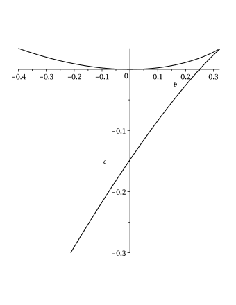
Figure 1. The discriminant set of the family of polynomials $x^{3}+x^{2}+bx+c$ and the sets $\Pi^{*}_{3,\sigma}\cap\{a=1\}$.

Example 3.

For $d=3$ (hence $\sigma=(\sigma_{0},\sigma_{1},\sigma_{2})$), we set $a_{2}:=a$, $a_{1}:=b$, $a_{0}:=c$, and we consider the polynomial $Q_{3}:=x^{3}+ax^{2}+bx+c$. Taking into account the group of quasi-homogeneous dilatations which preserves the discriminant set (see part (2) of Remarks 1) one concludes that each set $\Pi^{*}_{3,\sigma}$ is diffeomorphic to the corresponding direct product

$$(\Pi^{*}_{3,\sigma}\cap\{a=1\})\times(0,\infty)~{}~{}~{}{\rm if}~{}~{}~{}\sigma_{2}=+~{}~{}~{}{\rm or}~{}~{}~{}(\Pi^{*}_{3,\sigma}\cap\{a=-1\})\times(-\infty,0)~{}~{}~{}{\rm if}~{}~{}~{}\beta_{2}=-~{}.$$

Set $\sigma^{\prime}:=(-\sigma_{0},\sigma_{1},-\sigma_{2})$. Using the same group of dilatations with $u=-1$ one deduces that the set $\Pi^{*}_{3,\sigma^{\prime}}\cap\{a=-1\}$ is diffeomorphic to the set $\Pi^{*}_{3,\sigma}\cap\{a=1\}$. Therefore in order to prove that all sets $\Pi^{*}_{3,\sigma}$ are contractible it suffices to show this for the sets $\Pi^{*}_{3,\sigma}\cap\{a=1\}$ with $\sigma_{2}=+$. The latter sets are shown in Fig. 1. The figure represents the discriminant set of the polynomial $Q_{3}^{\bullet}:=x^{3}+x^{2}+bx+c$, i. e. the set

$${\rm Res}(Q_{3}^{\bullet},{Q_{3}^{\bullet}}^{\prime},x)=4b^{3}-b^{2}-18bc+27c^{2}+4c=0~{}.$$

(The set $\Delta_{3}^{2}$ is empty, because there is not more than one complex conjugate pair of roots, so $\Delta_{3}=\Delta_{3}^{1}$, see Remarks 1.) This is a curve in $\mathbb{R}^{2}:=Obc$ having a cusp at $(b,c)=(1/3,1/27)$ which corresponds to the polynomial $(x+1/3)^{3}$. The four sets $\Pi^{*}_{3,\sigma}\cap\{a=1\}$ are the intersections of the interior of the curve with the open coordinate quadrants. The intersections with $\{b>0,c>0\}$ and $\{b>0,c<0\}$ are bounded curvilinear triangles.

4. Proof of Theorem 1

Part (1). Each set $\mathcal{E}_{d}(\sigma)$ is non-empty. Indeed, given a polynomial $Q_{d}$ with $a_{0}>0$ (see Remark 2), for $C>0$ large enough, the polynomial $Q_{d}+C$ is elliptic. If the polynomials $Q_{d,1}$ and $Q_{d,2}$ belong to the set $\mathcal{E}_{d}(\sigma)$, then for $t\in[0,1]$, the polynomial $Q^{\sharp}_{d}:=tQ_{d,1}+(1-t)Q_{d,2}$ also belongs to it. Indeed, the signs of the respective coefficients are the same and if $Q_{d,1}(x)>0$ and $Q_{d,2}(x)>0$, then $Q^{\sharp}_{d}(x)>0$. Thus the set $\mathcal{E}_{d}(\sigma)$ is convex hence contractible.

Part (2). Each set $\mathcal{F}_{d}(\sigma)$ is non-empty. Indeed, for $C>0$ large enough, the polynomial $Q_{d}+{\rm sign}(a_{0})C$ has a single real root which is simple and the sign of this root is opposite to the sign of $Q_{d}(0)$. For a given polynomial $Q_{d}\in\mathcal{F}_{d}(\sigma)$, denote this root by $\xi$. Hence the polynomial $Q^{0}_{d}:=|\xi|^{d}Q_{d}(x/|\xi|)$ is in $\mathcal{F}_{d}(\sigma)$ and has a root at $1$ or $-1$. Suppose that the root is at $1$ (for $-1$ the proof is similar). We show that the subset $\mathcal{F}^{0}_{d}(\sigma)$ of $\mathcal{F}_{d}(\sigma)$ consisting of such polynomials $Q_{d}^{0}$ is convex hence contractible. On the other hand the set $\mathcal{F}_{d}(\sigma)$ is diffeomorphic to $\mathcal{F}^{0}_{d}(\sigma)\times\mathbb{R}^{*}_{+}$ from which contractibility of $\mathcal{F}_{d}(\sigma)$ follows.

For any two polynomials $Q_{d}^{0,\dagger}$, $Q_{d}^{0,*}\in\mathcal{F}^{0}_{d}(\sigma)$, the signs of the coefficients of the polynomial

$$Q^{0,\flat}_{d}:=tQ_{d}^{0,\dagger}+(1-t)Q_{d}^{0,*},~{}t\in[0,1],$$

are the same as the signs of the respective coefficients of $Q_{d}^{0,\dagger}$ and $Q_{d}^{0,*}$, so $Q^{0,\flat}_{d}\in\mathcal{F}^{0}_{d}(\sigma)$. This proves that $\mathcal{F}^{0}_{d}(\sigma)$ is convex.

Part (3).

A) Contractibility of the sets $\mathcal{G}_{d,(2,0)}(\sigma)$ and $\mathcal{G}_{d,(0,2)}(\sigma)$.

The two real roots of $Q_{d}$ have the same sign (i. e. $a_{0}>0$). We assume that they are positive, i. e. we prove contractibility only of $\mathcal{G}_{d,(2,0)}(\sigma)$; otherwise one can consider the polynomial $Q_{d}(-x)$ with the $d$-tuple $\tilde{\sigma}$ resulting from $\sigma$ via $x\mapsto-x$ (this mapping induces a bijection of the set of $d$-tuples onto itself) and contractibility of $\mathcal{G}_{d,(0,2)}(\tilde{\sigma})$ will be proved in the same way. Denote the real roots of $Q_{d}$ by $0<\xi<\eta$.

We can assume that at least one coefficient of odd degree of $Q_{d}$ is negative. Indeed, if all coefficients of $Q^{0}_{d}$ of odd degree are positive, then by Descartes’ rule of signs the polynomial $Q^{0}_{d}$ can have two real positive roots only if there is at least one coefficient of even degree which is negative. However in this case (and this is Case 1)) the set $\mathcal{G}_{d,(2,0)}(\sigma)$ is empty, see Proposition 4 in [7].

Next, we assume that $\eta=1$ (hence $\xi\in(0,1)$). Indeed, if one considers instead of $Q_{d}\in\mathcal{G}_{d,(2,0)}(\sigma)$ the polynomial $Q^{0}_{d}:=\eta^{d}Q_{d}(x/\eta)$, one has $Q^{0}_{d}\in\mathcal{G}_{d,(2,0)}(\sigma)$ and $Q^{0}_{d}(1)=0$. We denote the set of such polynomials $Q^{0}_{d}$ by $\mathcal{G}^{0}_{d,(2,0)}(\sigma)$. As $\mathcal{G}_{d,(2,0)}(\sigma)$ is diffeomorphic to $\mathcal{G}^{0}_{d,(2,0)}(\sigma)\times\mathbb{R}^{*}_{+}$, contractibility of $\mathcal{G}^{0}_{d,(2,0)}(\sigma)$ implies the one of $\mathcal{G}_{d,(2,0)}(\sigma)$.

For $\xi^{*}\in(0,1)$, we denote by $\mathcal{G}^{0,\xi^{*}}_{d,(2,0)}(\sigma)$ the subset of polynomials of $\mathcal{G}^{0}_{d,(2,0)}(\sigma)$ with $\xi=\xi^{*}$. If $Q^{0,1}_{d}$ and $Q^{0,2}_{d}$ are two polynomials of $\mathcal{G}^{0,\xi^{*}}_{d,(2,0)}(\sigma)$, then for $t\in[0,1]$, one has $tQ^{0,1}_{d}+(1-t)Q^{0,2}_{d}\in\mathcal{G}^{0,\xi^{*}}_{d,(2,0)}(\sigma)$. Therefore for each $\xi\in(0,1)$, the set $\mathcal{G}^{0,\xi}_{d,(2,0)}(\sigma)$ is convex hence contractible, and to prove contractibility of $\mathcal{G}^{0}_{d,(2,0)}(\sigma)$ (and hence of $\mathcal{G}_{d,(2,0)}(\sigma)$) it suffices to find for each $\xi\in(0,1)$ a polynomial $Q^{0,\xi}_{d}\in\mathcal{G}^{0,\xi}_{d,(2,0)}(\sigma)$ depending continuously on $\xi$.

Suppose that $m$ is odd, $1\leq m\leq d-1$, and that the coefficient of $Q_{d}\in\mathcal{G}_{d,(2,0)}(\sigma)$ of $x^{m}$ must be negative. There exists a unique polynomial of the form

(4.1) $$R:=x^{d}-Ax^{m}+B~{},~{}~{}~{}A>0~{},~{}~{}~{}B>0~{},~{}~{}~{}{\rm such~{}that}~{}~{}~{}R(\xi)=R(1)=0~{}.$$

Indeed, the conditions

(4.2) $$\xi^{d}-A\xi^{m}+B=1-A+B=0$$

imply

(4.3) $$A=(1-\xi^{d})/(1-\xi^{m})>0~{}~{}~{}{\rm and}~{}~{}~{}B=-1+A=\xi^{m}(1-\xi^{d-m})/(1-\xi^{m})>0~{}.$$

Remarks 4.

(1) The fractions for $A$, $B$ and $B/\xi^{m}$ can be extended by continuity for $\xi=0$ and $\xi=1$. For $\xi\in[0,1]$, one has

(4.4) $$\begin{array}[]{lll}A\in[1,\frac{d}{m}]~{},&\lim_{\xi\rightarrow 0^{+}}A=1~{},&\lim_{\xi\rightarrow 1^{-}}A=\frac{d}{m}~{},\\ \\ B\in[0,\frac{d-m}{m}]~{},&\lim_{\xi\rightarrow 0^{+}}B=0^{+}~{},&\lim_{\xi\rightarrow 1^{-}}B=\frac{d-m}{m}~{},\\ \\ B/\xi^{m}\in[0,{\rm max}(\frac{d-m}{m},1)]~{},&\lim_{\xi\rightarrow 0^{+}}B/\xi^{m}=1~{},&\lim_{\xi\rightarrow 1^{-}}B/\xi^{m}=\frac{d-m}{m}~{}.\end{array}$$

(2) The function $R$ has a global minimum at some point $x_{M}=x_{M}(\xi)\in(0,1)$. One has

$$\lim_{\xi\rightarrow 0^{+}}x_{M}(\xi)=x_{M,0}=(m/d)^{1/(d-m)}\in(0,1)~{},~{}~{}~{}R(x_{M,0})<0~{}~{}~{}{\rm and}~{}~{}~{}\lim_{\xi\rightarrow 1^{-}}x_{M}(\xi)=1~{}.$$

For $m\geq 3$, the tangent line to the graph of $R$ for $x=0$ is horizontal and $(0,R(0))$ is an inflection point. There is also another inflection point $x_{I}=x_{I}(\xi)\in(0,x_{M})$.

Set

(4.5) $$\mathcal{I}:=\{1,2,,\ldots,m-1,m+1,m+2,\ldots,d-1\}~{}.$$

We construct a polynomial $\Psi:=\sum_{j=0}^{d-1}\psi_{j}x^{j}$ with signs of the coefficients $\psi_{j}$, $j\in\mathcal{I}$, as defined by the $d$-tuple $\sigma$ and satisfying the conditions

(4.6) $$\Psi(\xi)=\Psi(1)=0~{}.$$

The latter conditions can be considered as a linear system with unknown variables $\psi_{0}$ and $\psi_{m}$. Its determinant equals $\xi^{m}-1\neq 0$, so for given $\psi_{j}$, $j\in\mathcal{I}$, these conditions define a unique couple $(\psi_{0},\psi_{m})$ whose signs are not necessarily the ones defined by the $d$-tuple $\sigma$. So to construct $\Psi$ it suffices to fix $\psi_{j}$ for $j\in\mathcal{I}$.

For each $\xi\in(0,1)$ fixed and for $\varepsilon>0$ sufficiently small, one has $R+\varepsilon\Psi\in\mathcal{G}^{0,\xi}_{d,(2,0)}(\sigma)$. Indeed, for $m\neq j\neq 0$, the coefficients of $R+\varepsilon\Psi$ have the signs defined by the $d$-tuple $\sigma$, so one has to check two things:

1) If $\varepsilon$ is small enough, then

(4.7) $$-A+\varepsilon\psi_{m}<0~{}~{}~{}{\rm and}~{}~{}~{}B+\varepsilon\psi_{0}>0~{}.$$

To obtain these two conditions simultaneously for all $\xi\in(0,1)$, one has to choose $\varepsilon$ as a function of $\xi$.

The conditions (4.6) can be given the form

$$\xi^{m}\psi_{m}+\psi_{0}=U~{},~{}\psi_{m}+\psi_{0}=V~{},$$

where $U$ and $V$ are polynomials in $\xi$ of degree $\leq d-1$. Hence

(4.8) $$\psi_{0}=(U-\xi^{m}V)/(1-\xi^{m})~{}~{}~{}{\rm and}~{}~{}~{}\psi_{m}=(V-U)/(1-\xi^{m})~{}.$$

Formulas (4.8) imply that $\Psi$ is of the form

(4.9) $$K(x,\xi)/(1-\xi)^{m}~{},~{}~{}~{}K\in\mathbb{R}[x,\xi]~{},~{}~{}~{}{\rm deg}_{x}K\leq d-1~{}.$$

As $\xi\rightarrow 0^{+}$, the quantity $B$ decreases as $\xi^{m}$, see (4.3) and (4.4). As $\xi\rightarrow 1^{-}$, the quantities $|\psi_{0}|$ and $|\psi_{m}|$ increase not faster than $C/(1-\xi)$ for some $C>0$. So to obtain $\varepsilon=\varepsilon(\xi)$ such that conditions (4.7) hold for $\xi\in(0,1)$, it suffices to set $\varepsilon:=c\xi^{m+1}(1-\xi)^{3}$ for some $c>0$ small enough.

2) For $\xi\in(0,1)$, one must have

(4.10) $$R+\varepsilon\Psi>0~{}~{}~{}{\rm for}~{}~{}~{}x\in(-\infty,\xi)\cup(1,\infty),~{}~{}~{}{\rm and}~{}~{}~{}R+\varepsilon\Psi<0~{}~{}~{}{\rm for}~{}~{}~{}x\in(\xi,1)~{}.$$

Lemma 1.

It is possible to choose $c>0$ so small that conditions (4.7) and (4.10) hold true simultaneously.

The lemma implies that for such $c>0$, $R+\varepsilon(\xi)\Psi\in\mathcal{G}^{0,\xi}_{d,(2,0)}(\sigma)$. So one can set $Q^{0,\xi}_{d}:=R+\varepsilon(\xi)\Psi$ from which contractibility of $\mathcal{G}_{d,(2,0)}(\sigma)$ follows.

Proof of Lemma 1.

Conditions (4.7) were already discussed, so we focus on conditions (4.10). Lowercase indices $\xi$ indicate differentiations w.r.t. $\xi$.

a) To obtain the condition $R+\varepsilon\Psi>0$ for $x>1$, it suffices to get $(R+\varepsilon\Psi)^{\prime}>0$ for $x\geq 1$. For $x\geq 1$, one has

(4.11) $$R^{\prime}=dx^{d-1}-mAx^{m-1}=x^{m-1}(dx^{d-m}-mA)\geq x^{m-1}(d-mA)$$

(as $R^{\prime}(1)>0$, one knows that $d-mA>0$). Next,

$$d-mA=\Lambda/(1-\xi^{m})~{},~{}~{}~{}\Lambda:=d-m+m\xi^{d}-d\xi^{m}~{}.$$

There exists $\alpha>0$ such that for $\xi\in[0,1]$, $\Lambda\geq\alpha(1-\xi)^{2}$. Indeed, $\Lambda_{\xi}=dm(\xi^{d-1}-\xi^{m-1})\leq 0$, with equality only for $\xi=0$ and $\xi=1$, so $\Lambda$ is strictly decreasing on $[0,1]$. The existence of $\alpha$ follows from

$$\begin{array}[]{ll}\Lambda(0)=d-m>0~{},~{}~{}~{}\Lambda(1)=\Lambda_{\xi}(1)=0&{\rm and}\\ \\ \Lambda_{\xi\xi}=dm((d-1)\xi^{d-1}-(m-1)\xi^{m-1})&{\rm hence}\\ \\ \Lambda_{\xi\xi}(1)=dm(d-m)>0~{}.&\end{array}$$

Thus for $\xi\in(0,1)$ and $x>1$, one has

$$R\geq(x^{m}/m)\alpha(1-\xi)^{2}/(1-\xi^{m})~{}~{}~{}\,{\rm and}~{}~{}~{}\,\varepsilon(\xi)\Psi\leq c\xi^{m+1}(1-\xi)^{3}K(x,\xi)/(1-\xi^{m})~{},$$

see (4.9). One can choose $c>0$ sufficiently small so that for $x\in(1,2]$, $R+\varepsilon\Psi>0$. There exists $\beta>0$ such that for $x\geq 2$, $dx^{d-m}-mA>\beta x^{d-m}$ (see (4.11) and (4.4)), so $R\geq\beta x^{d}/d$ and for $c>0$ small enough, $R+\varepsilon\Psi>0$.

b) For $x\leq-1$ (resp. for $x\in[-1,0]$), one has

$$R\geq|x|^{m}(|x|^{d-m}+A)~{}~{}~{}\,{\rm(resp.}~{}~{}~{}\,R\geq B\geq({\rm max}((d-m)/m,1))\xi^{m}{\rm)}$$

(see (4.1) and (4.4)) which for $c>0$ small enough is larger than $|\varepsilon(\xi)\Psi|$ and (4.10) holds true.

c) Suppose that $x\in(0,\xi)$. Then $R\geq\min(h(x,\xi),q(x,\xi))$, where

$$\tau~{}:~{}y=h(x,\xi):=R^{\prime}(\xi)(x-\xi)~{}~{}~{}\,{\rm and}~{}~{}~{}\,\chi~{}:~{}y=q(x,\xi):=B-Bx/\xi$$

are the tangent line to the graph of $R$ at the point $(\xi,0)$ and the line joining the points $(0,B)$ and $(\xi,0)$ respectively. Indeed, if $x_{I}\in[\xi,1)$ (see part (2) of Remarks 4), then the graph of $R$ is concave for $x\in[0,\xi]$, so it is situated above the line $\chi$. If $x_{I}\in(0,\xi)$, then for $x\in[x_{I},\xi]$, one has $R\geq h(x,\xi)$ and for $x\in(0,x_{I}]$, one has $R\geq q_{1}(x,\xi)$, where

$$\chi_{1}~{}:~{}y=q_{1}(x,\xi):=R(x_{I})+(x-x_{I})(R(x_{I})-B)/x_{I}$$

is the line joining the points $(0,B)$ and $(x_{I},R(x_{I}))$. The line $\chi_{1}$ is above the line $\chi$ for $x\in(0,x_{I})$.

Consider the smaller in absolute value of the slopes of the lines $\tau$ and $\chi$, i.e. $\mu:=\min(|R^{\prime}(\xi)|,B/\xi)$. One finds that

$$R^{\prime}(\xi)=\xi^{m-1}g(\xi)/(1-\xi^{m})~{},~{}~{}~{}g:=d\xi^{d-m}-m-(d-m)\xi^{d}~{},$$

with $g_{\xi}=d(d-m)(\xi^{d-m-1}-\xi^{d-1})\geq 0$, with equality only for $\xi=0$ and $\xi=1$. As $g(0)=-m<0$, $g(1)=0$,

$$g_{\xi\xi}=d(d-m)((d-m-1)\xi^{d-m-2}-(d-1)\xi^{d-2})~{},~{}~{}~{}\,{\rm so}~{}~{}~{}\,g_{\xi\xi}(1)=-md(d-m)<0~{},$$

there exists $\tilde{\beta}>0$ such that for $\xi\in(0,1)$, $|R^{\prime}(\xi)|\geq\tilde{\beta}\xi^{m-1}(1-\xi)^{2}/(1-\xi^{m})$. On the other hand $B/\xi=\xi^{m-1}(1-\xi^{d-m})/(1-\xi^{m})$. Thus $\mu\geq\mu_{0}:=\gamma\xi^{m-1}(1-\xi)$ for some $\gamma>0$. Hence for $x\in(0,\xi)$, the graph of $R$ is above the line $\delta:y=-\mu_{0}(x-\xi)$.

There exists $D_{0}>0$ such that for $\xi\in(0,1)$ and $x\in[0,1]$, one has $|(1-\xi)\Psi^{\prime}|\leq D_{0}$, see (4.8). Hence if $c>0$ is sufficiently small, the graph of $\varepsilon\Psi$ is below the line $\delta$ for $x\in[0,\xi)$, so $R+\varepsilon\Psi>0$.

d) Suppose that $m\geq 3$ and that $\xi>0$ is close to $0$. Then for $x>\xi$, the line $\tilde{\tau}$, which is tangent to the graph of $R$ at the point $(\xi,0)$, is above the straight line $\tilde{\rho}$ joining the points $(\xi,0)$ and $(x_{M},R(x_{M}))$. Indeed,

$$R^{\prime}(\xi)=\xi^{m-1}(d\xi^{d-m}-m-(d-m)\xi^{d})/(1-\xi^{m})=O(\xi^{m-1})$$

whereas the slope of $\tilde{\rho}$ is close to $R(x_{M,0})/x_{M,0}<0$. Therefore for $x\in(\xi,x_{M}]$, the graph of $R$ is below the line $\tilde{\tau}$.

For $x\in[x_{M},1)$, the graph of $R$ is below the line $\tilde{\chi}$ joining the points $(x_{M},R(x_{M}))$ and $(1,0)$ whose slope $-R(x_{M})/(1-x_{M})$ is close to $-R(x_{M,0})/(1-x_{M,0})>0$. On the other hand one has $|(1-\xi)\Psi^{\prime}|\leq D_{0}$ (see c)), so $|\varepsilon(\xi)\Psi^{\prime}|\leq c\xi^{m+1}(1-\xi)^{2}D_{0}$. Thus the graph of $\varepsilon(\xi)\Psi$ is above the line $\tilde{\tau}$ for $x\in(\xi,x_{M}]$ and above $\tilde{\chi}$ for $x\in[x_{M},1)$, hence it is between the graph of $R$ and the $x$-axis for $x\in(\xi,1)$, so $R+\varepsilon\Psi<0$.

e) For $m\geq 3$, we fix $\theta_{0}>0$ small enough such that for $\xi\in(0,\theta_{0}]$, $R+\varepsilon\Psi<0$, see d). For $m\geq 3$, $\xi\in[\theta_{0},1]$, $x\in(\xi,1)$, and for $m=1$, $\xi\in[0,1]$, $x\in(\xi,1)$, one has $R+\varepsilon(\xi)\Psi<0$ if $c>0$ is small enough. Indeed, one can write

$$R=(x-1)(x-\xi)R_{1}~{}~{}~{}\,{\rm and}~{}~{}~{}\,\Psi=(x-1)(x-\xi)\Psi_{1}~{},~{}~{}~{}R_{1},~{}\Psi_{1}\in\mathbb{R}[x,\xi]~{}.$$

Then $R_{1}(x,\xi)>0$. In particular, for $\xi=1$, one obtains

$$R=x^{d}-(d/m)x^{m}+(d-m)/m~{},~{}~{}~{}\,R^{\prime}=dx^{d-1}-dx^{m-1}~{},~{}~{}~{}\,{\rm so}~{}~{}~{}\,R^{\prime}(1)=0~{},$$

and $R^{\prime\prime}=d((d-1)x^{d-2}-(m-1)x^{m-2})$ hence $R^{\prime\prime}(1)=d(d-m)>0$, i. e. $R$ is divisible by $(x-1)^{2}$, but not by $(x-1)^{3}$.

For $m=1$, $\xi=0$, one has $R^{\prime}(0)<0$ (whereas for $m=3$, $\xi=0$, one has $R^{\prime}(0)=0$), this why for $m=1$ our reasoning is valid for $\xi\in[0,1]$, not only for $\xi\in[\theta_{0},1]$.

Denote by $R_{1,0}>0$ the minimal value of $R_{1}$ and by $\Psi_{1,0}$ the maximal value of $\Psi_{1}$ for $x\in[0,1]$. One can choose $c>0$ so small that for $x\in(\xi,1)$ and for the values of $\xi$ mentioned at the beginning of e),

$$R_{1}-\varepsilon\Psi_{1}\geq R_{1,0}-\varepsilon\Psi_{1,0}>0~{},~{}~{}~{}\,{\rm so}~{}~{}~{}\,R+\varepsilon\Psi<0~{},~{}~{}~{}\,{\rm because}~{}~{}~{}\,(x-1)(x-\xi)<0~{}.$$

The proof of the lemma results from a) – e). ∎

B) Contractibility of the set $\mathcal{G}_{d,(1,1)}(\sigma)$.

The two real roots of $Q_{d}$ have opposite signs (hence $a_{0}<0$). Denote them by $-\eta<0<\xi$. We define the sets

$$\mathcal{K}:=\mathcal{G}_{d,(1,1)}(\sigma)\cap\{\xi>\eta\}~{},~{}~{}~{}\mathcal{L}:=\mathcal{G}_{d,(1,1)}(\sigma)\cap\{\xi<\eta\}~{}~{}~{}{\rm and}~{}~{}~{}\mathcal{M}:=\mathcal{G}_{d,(1,1)}(\sigma)\cap\{\xi=\eta\}~{}.$$

Lemma 2.

Set $\sigma:=(\sigma_{0},\ldots,\sigma_{d-1})$, $\sigma_{j}=+$ or $-$.

(1) Suppose that $\sigma_{2j+1}=+$, $j=0$, $1$, $\ldots$, $(d/2)-1$. Then $\mathcal{K}=\mathcal{M}=\emptyset$.

(2) Suppose that $\sigma_{2j+1}=-$, $j=0$, $1$, $\ldots$, $(d/2)-1$. Then $\mathcal{L}=\mathcal{M}=\emptyset$.

(3) Suppose that there exist two odd integers $j_{1}\neq j_{2}$, $1\leq j_{1},j_{2}\leq d-1$, such that $\sigma_{j_{1}}=-\sigma_{j_{2}}$. Then all three sets $\mathcal{K}$, $\mathcal{L}$ and $\mathcal{M}$ are non-empty. There exists an open $d$-dimensional ball $\mathcal{B}\subset\mathcal{G}_{d,(1,1)}(\sigma)$ centered at a point in $\mathcal{M}$ and such that $\mathcal{B}\cap\mathcal{K}\neq\emptyset$ and $\mathcal{B}\cap\mathcal{L}\neq\emptyset$.

Proof.

Parts (1) and (2). If $\sigma_{2j+1}=+$ (resp. $\sigma_{2j+1}=-$), $j=0$, $1$, $\ldots$, $(d/2)-1$, then for a polynomial $Q_{d}\in\mathcal{G}_{d,(1,1)}(\sigma)$, one has $Q_{d}(0)<0$ and $Q_{d}(a)>Q_{d}(-a)$ (resp. $Q_{d}(0)<0$ and $Q_{d}(a)<Q_{d}(-a)$) for $a>0$. Hence $\xi<\eta$ (resp. $\xi>\eta$).

Part (3). We construct a polynomial $Q_{d}^{\diamond}\in\mathcal{M}$. Set $u:=\xi^{j_{1}-j_{2}}$ and

$$Q_{d}^{\diamond}:=x^{d}-\xi^{d}+\sigma_{j_{1}}(x^{j_{1}}-ux^{j_{2}})+\varepsilon(Q_{d}^{\diamond,o}+Q_{d}^{\diamond,e})~{},$$

where

$$Q_{d}^{\diamond,e}=b+\sum_{j=1}^{d/2}\sigma_{2j}x^{2j}~{},~{}~{}~{}b\in\mathbb{R}~{},~{}~{}~{}Q_{d}^{\diamond,o}=rx^{j_{1}}+\sum_{j=0}^{d/2-1}\sigma_{2j+1}x^{2j+1}$$

and $\varepsilon>0$ is small enough. We choose $b$ and $r$ such that $Q_{d}^{\diamond,e}(\pm\xi)=0$ and $Q_{d}^{\diamond,o}(\pm\xi)=0$ respectively. Then $Q_{d}^{\diamond}(\pm\xi)=0$ and for $j\neq 0$ and $j_{1}\neq j\neq j_{2}$, the sign of the coefficients of $x^{j}$ of $Q_{d}^{\diamond}$ is as defined by $\sigma$. For $\varepsilon>0$ small enough, one has sign$(Q_{d}^{\diamond}(0))$=sign$(-\xi^{d}+\varepsilon b)=-$. The coefficient of $x^{j_{1}}$ (resp. $x^{j_{2}}$) of $Q_{d}^{\diamond}$ equals $\sigma_{j_{1}}\times(1+\varepsilon(1+r))$ (resp. $\sigma_{j_{2}}\times(u+\varepsilon(1+r))$), so it has the same sign as $\sigma_{j_{1}}$ (resp. as $\sigma_{j_{2}}$).

Consider a $d$-dimensional ball $\mathcal{B}$ centered at a point $Q_{d}^{\diamond}\in\mathcal{M}$, with $\xi=\eta=\xi_{0}$ and belonging to $\mathcal{G}_{d,(1,1)}(\sigma)$. Perturb the real root $\xi$ of $Q_{d}^{\diamond}$ so that it takes values smaller and values larger than $\xi_{0}$. The signs of the coefficients of $Q_{d}^{\diamond}$ do not change. Hence $\mathcal{B}$ intersects $\mathcal{K}$ and $\mathcal{L}$. ∎

We show first that each of the two sets $\mathcal{K}$ and $\mathcal{L}$, when nonempty, is contractible. If we are in the conditions of part (1) or (2) of Lemma 2, then this implies contractibility of $\mathcal{G}_{d,(1,1)}(\sigma)$. When we are in the conditions of part (3), then one can contract $\mathcal{K}$ and $\mathcal{L}$ into points of $\mathcal{B}$ and then contract $\mathcal{B}$ into a point, so in this case $\mathcal{G}_{d,(1,1)}(\sigma)$ is also contractible.

We prove contractibility only of $\mathcal{K}$ (when non-empty). The one of $\mathcal{L}$ is performed by complete analogy (the change of variable $x\mapsto-x$ exchanges the roles of $\mathcal{K}$ and $\mathcal{L}$ and changes the $d$-tuple $\sigma$ accordingly). So we suppose that $\xi>\eta$. As in the proof of A) we reduce the proof of the contractibility of $\mathcal{K}$ to the one of the contractibility of $\mathcal{K}\cap\{\xi=1\}$. As in A) we observe that if

$$Q^{\ddagger}_{d}~{},~{}~{}~{}Q^{\triangle}_{d}\in\mathcal{K}^{\eta^{*}}:=\mathcal{K}\cap\{\xi=1,\eta=\eta^{*}\in(0,1)\}~{},$$

then $tQ^{\ddagger}_{d}+(1-t)Q^{\triangle}_{d}\in\mathcal{K}^{\eta^{*}}$, so $\mathcal{K}^{\eta^{*}}$ is convex hence contractible and contractibility of $\mathcal{K}\cap\{\xi=1\}$ (and also of $\mathcal{K}$) will be proved if we construct for each $\eta\in(0,1)$ a polynomial $Q_{d}\in\mathcal{K}^{\eta}$ depending continuously on $\eta$.

Suppose that there is a negative coefficient of $Q_{d}$ of odd degree $m$ (otherwise $\mathcal{K}$ is empty). For $\eta\in(0,1)$, we construct a polynomial

$$S:=x^{d}-\tilde{A}x^{m}-\tilde{B}~{},~{}~{}~{}\tilde{A}>0~{},~{}~{}~{}\tilde{B}>0~{},~{}~{}~{}{\rm such~{}that}~{}~{}~{}S(1)=S(-\eta)=0~{}.$$

The latter two equalities imply

(4.12) $$\tilde{A}=(1-\eta^{d})/(1+\eta^{m})>0~{}{\rm and}~{}\tilde{B}=\eta^{m}(1+\eta^{d-m})/(1+\eta^{m})>0~{}.$$

Remarks 5.

(1) Thus for $\eta\in[0,1]$, there exist constants $0<B_{{\rm min}}\leq B_{{\rm max}}$ such that $\tilde{B}/\eta^{m}\in[B_{{\rm min}},B_{{\rm max}}]$. Moreover one has

(4.13) $$\begin{array}[]{lll}\tilde{A}\in[0,1]~{},&\lim_{\eta\rightarrow 0^{+}}\tilde{A}=1~{},&\lim_{\eta\rightarrow 1^{-}}\tilde{A}=0^{+}~{},\\ \\ \tilde{B}\in[0,1]~{},&\lim_{\eta\rightarrow 0^{+}}\tilde{B}=0^{+}~{},&\lim_{\eta\rightarrow 1^{-}}\tilde{B}=1~{},\\ \\ \lim_{\eta\rightarrow 0^{+}}\tilde{B}/\eta^{m}=1&{\rm and}&\lim_{\eta\rightarrow 1^{-}}\tilde{B}/\eta^{m}=1~{}.\end{array}$$

(2) The derivative $S^{\prime}$ has a unique root $\tilde{x}_{M}$ (which is simple) in $(0,1)$. All non-constant derivatives of $S$ are increasing for $x>\tilde{x}_{M}$, have one or two roots (depending on $m$) in $[0,\tilde{x}_{M})$ and no root outside this interval.

We construct a polynomial $\Phi:=\sum_{j=0}^{d-1}\varphi_{j}x^{j}$, where for $j\in\mathcal{I}$ (see (4.5)), the sign of $\varphi_{j}$ is defined by the $d$-tuple $\sigma$. This polynomial must satisfy the condition

$$\Phi(-\eta)=\Phi(1)=0$$

which can be regarded as a linear system with known quantities $\varphi_{j}$, $j\in\mathcal{I}$, and with unknown variables $\varphi_{0}$ and $\varphi_{m}$:

(4.14) $$\begin{array}[]{lll}-\eta^{m}\varphi_{m}+\varphi_{0}=W~{},&\varphi_{m}+\varphi_{0}=T~{},&W,T\in\mathbb{R}[\eta]~{},~{}~{}~{}{\rm so}\\ \\ \varphi_{0}=(\eta^{m}T+W)/(1+\eta^{m})~{},&\varphi_{m}=(T-W)/(1+\eta^{m})~{}.&\end{array}$$

One must also have $S+\varepsilon_{1}(\eta)\Phi\in\mathcal{K}^{\eta}$, $\eta\in(0,1)$, for some suitably chosen positive-valued continuous function $\varepsilon_{1}(\eta)$. For $\varepsilon_{1}(\eta)>0$ small enough, the sign of the coefficient of $x^{j}$, $j\in\mathcal{I}$, of the polynomial $S+\varepsilon_{1}(\eta)\Phi$ is as defined by the $d$-tuple $\sigma$. So one needs to choose $\varepsilon_{1}(\eta)$ such that

(4.15) $$\tilde{A}+\varepsilon_{1}(\eta)\varphi_{m}<0~{},~{}-\tilde{B}+\varepsilon_{1}(\eta)\varphi_{0}<0$$

and

(4.16) $$S+\varepsilon_{1}(\eta)\Phi>0~{}~{}~{}\,{\rm for}~{}~{}~{}\,x\in(-\infty,-\eta)\cup(1,\infty)~{},~{}~{}~{}S+\varepsilon_{1}(\eta)\Phi<0~{}~{}~{}\,{\rm for}~{}~{}~{}\,x\in(-\eta,1)~{}.$$

We set $\varepsilon_{1}:=\tilde{c}\eta^{m}(1-\eta)^{2}$, $\tilde{c}>0$. If one chooses $\tilde{c}$ small enough, conditions (4.15) will hold true.

Lemma 3.

For $\tilde{c}>0$ small enough, conditions (4.16) hold true.

Contractibility of $\mathcal{K}$ follows from the lemma.

Proof of Lemma 3.

All derivatives of $S$ of order $\leq d-1$ are increasing functions in $x$ for $x\geq 1$ (see Remarks 5). As

$$S^{\prime}(1)=(d+d\eta^{m}-m+m\eta^{d})/(1+\eta^{m})\geq(d-m)/2~{},$$

one can choose $\tilde{c}$ small enough so that for $x\in[1,2]$, $S^{\prime}+\varepsilon_{1}(\eta)\Phi^{\prime}>0$. Hence $S+\varepsilon_{1}(\eta)\Phi>0$ for $x\in(1,2]$. If $x\geq 2$, then for some positive constants $k_{1}$ and $k_{2}$, one has $S^{\prime}\geq k_{1}x^{d-1}$ and $\Phi^{\prime}\leq k_{2}x^{d-2}$, so if $\tilde{c}>0$ is small enough, then for $x\geq 2$ (hence for $x>1$), $S^{\prime}+\varepsilon_{1}(\eta)\Phi^{\prime}>0$ and $S+\varepsilon_{1}(\eta)\Phi>0$.

One has

$$S^{\prime}(-\eta)=-(d\eta^{d-1}+(d-m)\eta^{d+m-1}+m\eta^{m-1})/(1+\eta^{m})=O(\eta^{m-1})~{},$$

$S^{\prime}(-\eta)<0$ and $S$ is convex for $x<0$. Hence one can choose $\tilde{c}>0$ so small that for $x\in[-2,-\eta]$, $S^{\prime}+\varepsilon_{1}(\eta)\Phi^{\prime}<0$ hence $S+\varepsilon_{1}(\eta)\Phi>0$. Indeed, for $\eta\in[0,1]$ and $x\in[-2,0]$, $\Phi^{\prime}$ is bounded. For $x\leq-2$, one has

$$S^{\prime}\leq k_{1}^{*}x^{d-1}~{}~{}~{}\,\,{\rm and}~{}~{}~{}\,\,|\Phi^{\prime}|\leq k_{2}^{*}x^{d-2}$$

for some positive constants $k_{1}^{*}$, $k_{2}^{*}$, so $S+\varepsilon_{1}(\eta)\Phi<0$ (thus this holds true for $x<-\eta$).

The function $S$ is convex on $[-\eta,0]$, see Remarks 5. Hence for $x\in[-\eta,0]$, the graph of $S$ is below the line $\zeta$ joining the points $(-\eta,0)$ and $(0,-\tilde{B})$. Its slope is $-\tilde{B}/\eta$, with $|-\tilde{B}/\eta|=O(\eta^{m-1})$. Hence for $x\in[-\eta,0]$ and for $\tilde{c}>0$ sufficiently small, the graph of $\Phi$ is above the line $\zeta$ (because $\Phi^{\prime}$ is bounded for $x\in[-1,0]$, $\eta\in[0,1]$) and one has $S+\varepsilon_{1}(\eta)\Phi<0$.

Suppose that $x\in[0,\tilde{x}_{M}]$. The function $S$ is decreasing, see Remarks 5, hence $S(x)\leq S(0)=-\tilde{B}=O(\eta^{m})$. As there exists $k_{3}>0$ such that for $x\in[0,1]$, $|\Phi|\leq k_{3}$, for $\tilde{c}>0$ sufficiently small, one has $S+\varepsilon_{1}(\eta)\Phi<0$.

For $x\in[\tilde{x}_{M},1]$, the function $S$ is convex. Hence its graph is below the line $\tilde{\zeta}$ joining the points $(\tilde{x}_{M},S(\tilde{x}_{M}))$ and $(1,0)$. Recall that $S(\tilde{x}_{M})\leq S(0)=-\tilde{B}=O(\eta^{m})$. There exists $k_{4}>0$ such that for $x\in[0,1]$ and $\eta\in[0,1]$, $|\Phi^{\prime}|\leq k_{4}$. Thus the slope of $\tilde{\zeta}$ is

$$\geq\tilde{B}/(1-\tilde{x}_{M})>\tilde{B}=O(\eta^{m})$$

while $|\varepsilon\Phi^{\prime}|\leq\tilde{c}\eta^{m}(1-\eta)^{2}k_{4}$. Hence for sufficiently small values of $\tilde{c}>0$, the graph of $\varepsilon\Phi$ is above the line $\tilde{\zeta}$ and $S+\varepsilon_{1}(\eta)\Phi<0$. ∎

5. Proofs of Theorems 2 and 3

Proof of Theorem 2.

In the proof we assume that the polynomials of $\Pi_{d}$ are of the form $Q_{d}:=x^{d}+a_{d-1}x^{d-1}+\cdots+a_{2}x^{2}+a_{1}x+a_{0}$ and the ones of $\Pi_{d-1}$ are of the form $Q_{d-1}:=x^{d-1}+a_{d-1}x^{d-2}+\cdots+a_{2}x+a_{1}$. Thus the intersection $\Pi_{d}\cap\{a_{0}=0\}$ can be identified with $\Pi_{d-1}$.

We show that every polynomial $Q_{d}\in\Pi_{d}^{*}$ can be continuously deformed so that it remains in $\Pi_{d}^{*}$, the signs of its coefficients do not change throughout the deformation except the one of $a_{0}$ which vanishes at the end of the deformation. Therefore

1) throughout the deformation the quantities of positive and negative roots do not change;

2) at the end of the deformation exactly one root vanishes and a polynomial of the form $xQ_{d-1}$ is obtained with $Q_{d-1}\in\Pi_{d}\cap\{a_{0}=0\}$.

Moreover, we show that throughout and at the end of the deformation one obtains polynomials with distinct real roots. Thus any given component of the set $\Pi_{d}^{*}$ can be retracted into a component of the set $\Pi_{d-1}^{*}$; the latter is defined by the $(d-1)$-tuple obtained from $\sigma$ by deleting its first component. For $d=2$, all components of the set $\Pi_{2}^{*}$ are contractible, see Example 2.

This means that for every given $d$ and $\sigma$, there exists exactly one component of $\Pi_{d}^{*}$, and which is contractible. The deformation mentioned above is defined like this:

$$Y_{d}:=(Q_{d}+txQ_{d}^{\prime})/(1+td)=\sum_{j=0}^{d}((1+tj)/(1+td))a_{j}x^{j}~{},~{}~{}~{}t\geq 0~{}.$$

It is clear that the polynomial $Y_{d}$ is monic, with sign$(a_{j})=$sign$((1+tj)a_{j}/(1+td))$ and $\lim_{t\rightarrow+\infty}((1+tj)a_{j}/(1+td))=ja_{j}/d$. There remains to prove only that $Y_{d}$ has $d$ distinct real roots.

Denote the roots of $Q_{d}$ by $\eta_{1}<\cdots<\eta_{s}<0<\xi_{1}<\cdots<\xi_{d-s}$. The polynomial $Q_{d}^{\prime}$ has exactly one root in each of the intervals $(\eta_{1},\eta_{2})$, $\ldots$, $(\eta_{s-1},\eta_{s})$, $(\eta_{s},\xi_{1})$, $(\xi_{1},\xi_{2})$, $\ldots$, $(\xi_{d-s-1},\xi_{d-s})$. We denote these roots by $\tau_{1}<\cdots<\tau_{d-1}$.

For each $t\geq 0$, the polynomial $Y_{d}$ changes sign in each of the intervals $(\eta_{j},\tau_{j})$, $j=1$, $\ldots$, $s-1$, and in each of the intervals $(\tau_{s+i-1},\xi_{i})$, $i=2$, $\ldots$, $d-s$, so it has a root there. This makes not less than $d-2$ distinct real roots.

If $\tau_{s}>0$ (resp. $\tau_{s}<0$), then $Y_{d}$ changes sign in each of the intervals $(\eta_{s},0)$ and $(\tau_{s},\xi_{1})$ (resp. $(\eta_{s},\tau_{s})$ and $(0,\xi_{1})$), so it has two more real distinct roots. Hence for any $t\geq 0$, $Y_{d}$ is hyperbolic, with $d$ distinct roots. ∎

Proof of Theorem 3.

We remind that we denote by $H^{k}_{\pm}$ not only the graphs mentioned in Theorem 4, but also the corresponding functions.

A) We prove Theorem 3 by induction on $d$. The induction base are the cases $d=2$ and $d=3$, see Examples 2 and 3.

Suppose that Theorem 3 holds true for $d=d_{0}\geq 3$. Set $d:=d_{0}+1$. As in the proof of Theorem 2 we set $Q_{d}:=x^{d}+a_{d-1}x^{d-1}+\cdots+a_{2}x^{2}+a_{1}x+a_{0}$ and $Q_{d-1}:=x^{d-1}+a_{d-1}x^{d-2}+\cdots+a_{2}x+a_{1}$, so that the intersection $\Pi_{d}\cap\{a_{0}=0\}$ can be identified with $\Pi_{d-1}$.

B) We remind that any stratum (or component) $U$ of $\Pi_{d-1}^{*}$ is of the form (see Notation 2 and Remark 4)

$$U=S_{1^{d-1}}(\sigma_{1},\ldots,\sigma_{d-1})=\{a^{\prime}\in S_{1^{d-1}}~{}|~{}{\rm sign}(a_{j})=\sigma_{j},1\leq j\leq d-1\}~{}.$$

Starting with such a component $U$ (hence $U=U^{d-1}$), we construct in several steps the components $U_{+}$ and $U_{-}$ of the set $\Pi_{d}^{*}$ sharing with $U$ the signs of the coefficients $a_{d-1}$, $\ldots$, $a_{1}$. One has $a_{0}>0$ in $U_{+}$ and $a_{0}<0$ in $U_{-}$.

At the first step we construct the sets $U_{1,\pm}$ as follows. We remind that the projections $\pi^{k}$ and their fibres $\tilde{f}_{k}$ were defined in part (1) of Theorem 4. Each fibre $\tilde{f}_{d}$ of the projection $\pi^{d}$ which is over a point of $U$ is a segment, see part (1) of Theorem 4. If $Q_{d-1}\in U$, then for $\varepsilon>0$ small enough, both polynomials $xQ_{d-1}\pm\varepsilon$ are hyperbolic. Indeed, all roots of $Q_{d-1}$ are real and simple. The set $U_{1,+}$ (resp. $U_{1,-}$) is the union of the interior points of these fibres $\tilde{f}_{d}$ which are with positive (resp. with negative) $a_{0}$-coordinates. Thus

$$\begin{array}[]{ll}U_{1,+}=\{a\in\tilde{f}_{d}~{}|~{}a^{\prime}\in U,~{}0<a_{0}<H^{d}_{+}(a^{\prime})\}&{\rm and}\\ \\ U_{1,-}=\{a\in\tilde{f}_{d}~{}|~{}a^{\prime}\in U,~{}H^{d}_{-}(a^{\prime})<a_{0}<0\}~{},&\end{array}$$

see part (6) of Theorem 4). Hence the sets $U_{1,\pm}$ are open, non-empty and contractible.

For $d\geq 2$, the intersection $\Pi_{d}\cap\{a_{0}=0\}$ is strictly included in the projection $\Pi_{d}^{d-1}$ of $\Pi_{d}$ in $Oa_{1}\cdots a_{d-1}$. Therefore one can expect that the sets $U_{1,\pm}$ are not the whole of two components of $\Pi_{d}^{*}$. We construct contractible sets $U_{1,\pm}\subset U_{2,\pm}\subset\cdots\subset U_{d-1,\pm}$, where for $1\leq j\leq d-1$, the signs of the coordinates $a_{j}$ of each point of $U_{k,+}$ (resp. $U_{k,-}$) are defined by $\sigma$, and $U_{d-1,\pm}$ are components of $\Pi_{d}^{*}$. One has $a_{0}>0$ in $U_{k,+}$ and $a_{0}<0$ in $U_{k,-}$.

C) Recall that the set $U$ consists of all the points between the graphs $L^{d-1}_{\pm}$ of two continuous functions defined on $U^{d-2}$:

$$U=\{a^{\prime}~{}|~{}L^{d-1}_{-}(a^{\prime\prime})<a^{\prime\prime}<L^{d-1}_{+}(a^{\prime\prime}),~{}a^{\prime\prime}\in U^{d-2}\}~{},$$

see Notation 2. Thus $(L^{d-1}_{+}\cup L^{d-1}_{-})\subset\partial U$. Depending on the sign of $a_{1}$ in $U$, for each of these graphs, part or the whole of it could belong to the hyperplane $a_{1}=0$.

Consider a fibre $\tilde{f}_{d}$ over a point of one of the graphs $L^{d-1}_{\pm}$ and not belonging to the hyperplane $a_{1}=0$. A priori the two endpoints of the fibre cannot have $a_{0}$-coordinates with opposite signs. Indeed, if this were the case for the fibre over $a^{\prime}={a^{*}}^{\prime}$ (see Notation 2), then for all fibres over $a^{\prime}$ close to ${a^{*}}^{\prime}$, these signs would also be opposite, because the functions $L^{d}_{\pm}$, whose values are the values of the $a_{0}$-coordinates of the endpoints, are continuous. Hence all these fibres $\tilde{f}_{d}$ intersect the hyperplane $a_{0}=0$ (see part (1) of Theorem 4), but not the hyperplane $a_{1}=0$. Hence the point ${a^{*}}^{\prime}$ is an interior point of $\Pi_{d}$ (hence of $U$ as well) and not a point of $\partial U$ which is a contradiction, see part (2) of Theorem 4.

Both endpoints cannot have non-zero coordinates of the same sign, because then in the same way the fibres $\tilde{f}_{d}$ over all points $a^{\prime}$ close to ${a^{*}}^{\prime}$ would not intersect the hyperplane $a_{0}=0$ hence ${a^{*}}^{\prime}\not\in\overline{U}$, so ${a^{*}}^{\prime}\not\in\partial U$.

Hence the following three possibilities remain:

a) both endpoints have zero $a_{0}$-coordinates;

b) one endpoint has a zero and the other endpoint has a positive $a_{0}$-coordinate;

c) one endpoint has a zero and the other endpoint has a negative $a_{0}$-coordinate.

D) Consider the points of the graph $L^{d-1}_{+}$ which do not belong to the hyperplane $a_{1}=0$ (for $L^{d-1}_{-}$ the reasoning is similar). If for $B\in(L^{d-1}_{+}\setminus\{a_{1}=0\})$, possibility a) takes place, then there is nothing to do.

Suppose that possibility b) takes place. Denote by $a_{j,B}$ the coordinates of the point $B$ (hence $a_{0,B}=0$). For each such point $B$, fix the coordinates $a_{j}=a_{j,B}$ for $j\neq 1$ and increase $a_{1}$. The interior points of the corresponding fibres $\tilde{f}_{d}$ (when non-void) have the same signs of their $a_{0}$-coordinates, hence these signs are positive. Then for some $a_{1}=a_{1,C}>a_{1,B}$, one has either $a_{1,C}=0$ (this can happen only when $a_{1,B}<0$) or the point $C$ belongs to the graph $H^{d-1}_{+}$ and for $a_{1}>a_{1,C}$, the fibres $\tilde{f}_{d}$ are void, see Theorem 4.

In both these situations we add to the set $U_{1,+}$ the points of the interior of all fibres $\tilde{f}_{d}$ over the interval $[a_{1,B},a_{1,C})$ (with $a_{j}=a_{j,B}$ for $j\neq 1$), over all points $B\in(L^{d-1}_{+}\setminus\{a_{1}=0\})$.

If possibility c) takes place, then we fix again $a_{j,B}$ for $j\neq 1$ and increase $a_{1}$. The interior points of the corresponding fibres $\tilde{f}_{d}$ (when non-void) have negative sign of their $a_{0}$-coordinates. We add to the set $U_{1,-}$ the interior points of all fibres $\tilde{f}_{d}$ over the interval $[a_{1,B},a_{1,C})$ (with $a_{j}=a_{j,B}$ for $j\neq 1$), over all points $B\in(L^{d-1}_{+}\setminus\{a_{1}=0\})$.

E) We perform a similar reasoning and construction with $L^{d-1}_{-}$ (in which the role of $H^{d-1}_{+}$ is played by $H^{d-1}_{-}$). In this case $a_{1}$ is to be decreased, one has $a_{1,C}<a_{1,B}$ and the interval $[a_{1,B},a_{1,C})$ is to be replaced by the interval $(a_{1,C},a_{1,B}]$.

F) Thus we have enlarged the sets $U_{1,\pm}$; the new sets are denoted by $U_{2,\pm}$:

$$\begin{array}[]{lll}U_{2,+}&=&U_{1,+}\cup\{a\in\Pi^{*}_{d}~{}|~{}a^{\prime\prime}\in U^{d-2},~{}L_{+}^{d-1}(a^{\prime\prime})<a_{1}<H^{d-1}_{+}(a^{\prime\prime}),\\ \\ &&{\rm if}~{}L_{+}^{d-1}(a^{\prime\prime})\geq 0,~{}L_{+}^{d-1}(a^{\prime\prime})<a_{1}<{\rm min}(0,H^{d-1}_{+}(a^{\prime\prime})),~{}{\rm if}~{}L_{+}^{d-1}(a^{\prime\prime})<0~{}\}~{},\\ \\ U_{2,-}&=&U_{1,-}\cup\{a\in\Pi^{*}_{d}~{}|~{}a^{\prime\prime}\in U^{d-2},~{}H^{d-1}_{-}(a^{\prime\prime})<a_{1}<L_{-}^{d-1}(a^{\prime\prime}),\\ \\ &&{\rm if}~{}L_{-}^{d-1}(a^{\prime\prime})\leq 0,~{}{\rm max}(0,H^{d-1}_{-}(a^{\prime\prime}))<a_{1}<L_{-}^{d-1}(a^{\prime\prime}),~{}{\rm if}~{}L_{-}^{d-1}(a^{\prime\prime})>0~{}\}~{}.\end{array}$$

The sets $U_{1,\pm}$ and $U_{2,\pm}$ satisfy the conclusion of Theorem 3. We denote the graphs $L^{k}_{\pm}$ defined for the sets $U_{1,\pm}$ and $U_{2,\pm}$ by $L^{k}_{1,\pm}$ and $L^{k}_{2,\pm}$. The construction of these graphs implies that they are graphs of continuous functions (because such are the graphs $H^{k}_{\pm}$). The set $U_{1,+}\cup U_{1,-}$ (resp. $U_{2,+}\cup U_{2,-}$) contains all points of the set $(\pi^{d})^{-1}(U)\cap\Pi_{d,\sigma}^{*}$ (resp. $(\pi^{d-1}\circ\pi^{d})^{-1}(U^{d-2})\cap\Pi_{d,\sigma}^{*}$).

G) We remind that $\tilde{f}_{d}=f^{\diamond}_{d-1}$, see Remark 5. Suppose that the sets $U_{s,\pm}$, $2\leq s\leq d-3$, are constructed such that they satisfy the conclusion of Theorem 3 (the graphs $L^{k}_{\pm}$ are denoted by $L^{k}_{s,\pm}$) and that the set $U_{s,+}\cup U_{s,-}$ contains all points of the set $(\pi^{d-s+1}\circ\cdots\circ\pi^{d})^{-1}(U^{d-s})\cap\Pi_{d,\sigma}^{*}$.

Consider a point $D\in L^{d-s}_{+}$ which does not belong to the hyperplane $a_{s}=0$. For the fibre $f^{\diamond}_{d-s}$ of the projection $\pi^{d-s+1}\circ\cdots\circ\pi^{d}$ which is over $D$ (see Remark 5) one of the three possibilities takes place:

a’) the minimal and the maximal possible value of the $a_{s}$-coordinate of the points of the fibre are zero;

b’) the minimal possible value is $0$ and the maximal possible value is positive;

c’) the minimal possible value is negative and the maximal possible value is $0$.

It is not possible to have both the maximal and minimal possible value of $a_{s}$ non-zero, because in this case the point $D$ does not belong to the set $\partial U^{d-s}$. This is proved by analogy with C). With regard to Remark 5, when the fibre $f^{\diamond}_{d-s}$ is not a point, then the maximal (resp. the minimal) value of $a_{s}$ is attained at one of the $0$-dimensional cells (resp. at the other $0$-dimensional cell) and only there. This can be deduced from part (2) of Theorem 4.

H) When possibility a’) takes place, then there is nothing to do. Suppose that possibility b’) takes place. Denote by $a_{j,D}$ the coordinates of the point $D$ (hence $a_{0,D}=\cdots=a_{s-1,D}=0$). Fix $a_{j,D}$ for $j\neq s$ and increase $a_{s}$. Then for some $a_{s}=a_{s,E}>a_{s,D}$, one has either $a_{s,E}=0$ (which is possible only if $a_{s,D}<0$) or the point $E$ belongs to the graph $H^{d-s}_{+}$. In this case we add to the set $U_{s,+}$ the points of the interior of all fibres $f^{\diamond}_{d-s}$ over the interval $[a_{s,D},a_{s,E})$ (with $a_{j}=a_{j,D}$ for $j\neq s$), over all points $D\in(L^{d-s}_{+}\setminus\{a_{s}=0\})$. The $a_{s-1}$-coordinates of all points thus added are positive.

If possibility c’) takes place, then we fix again $a_{j,D}$ for $j\neq s$ and increase $a_{s}$. We add to the set $U_{s,-}$ the points of the interior of all fibres $f^{\diamond}_{d-s}$ over the interval $[a_{s,D},a_{s,E})$ (with $a_{j}=a_{j,D}$ for $j\neq s$), over all points $D\in L^{d-s}_{+}\setminus\{a_{s}=0\}$. The $a_{s-1}$-coordinates of all points thus added are negative.

We consider in a similar way the graph $L^{d-s}_{-}$ in which case the role of $H^{d-s}_{+}$ is played by $H^{d-s}_{-}$, $a_{s}$ is to be decreased, one has $a_{s,E}<a_{s,D}$ and the interval $[a_{s,D},a_{s,E})$ is to be replaced by the interval $(a_{s,E},a_{s,D}]$.

I) We have thus constructed the sets $U_{s+1,\pm}$ which satisfy the conclusion of Theorem 3:

$$\begin{array}[]{lll}U_{s+1,+}&=&U_{s,+}\cup\{a\in\Pi^{*}_{d}~{}|~{}a^{(s+1)}\in U^{d-s-1},\\ \\ &&L_{s,+}^{d-s}(a^{(s+1)})<a_{s}<H^{d-s}_{+}(a^{(s+1)}),~{}{\rm if}~{}L_{s,+}^{d-s}(a^{(s+1)})\geq 0,\\ \\ &&L_{s,+}^{d-s}(a^{(s+1)})<a_{s}<{\rm min}(0,H^{d-s}_{+}(a^{(s+1)})),~{}{\rm if}~{}L_{s,+}^{d-s}(a^{(s+1)})<0~{}\}~{},\\ \\ U_{s+1,-}&=&U_{s,-}\cup\{a\in\Pi^{*}_{d}~{}|~{}a^{(s+1)}\in U^{d-s-1},\\ \\ &&H^{d-s}_{-}(a^{(s+1)})<a_{s}<L_{s,-}^{d-s}(a^{(s+1)}),~{}{\rm if}~{}L_{s,-}^{d-s}(a^{(s+1)})\leq 0,\\ \\ &&{\rm max}(0,H^{d-s}_{-}(a^{(s+1)}))<a_{s}<L_{s,-}^{d-s}(a^{(s+1)}),~{}{\rm if}~{}L_{s,-}^{d-s}(a^{(s+1)})>0~{}\}~{}.\end{array}$$

The set $U_{s+1,+}\cup U_{s+1,-}$ contains all points of the set $(\pi^{d-s}\circ\cdots\circ\pi^{d})^{-1}(U^{d-s-1})\cap\Pi_{d,\sigma}^{*}$. It should be noticed that as the fibres $f^{\diamond}_{d-s}$ contain cells of dimension from $0$ to $s$, all graphs $L_{s,\pm}^{k}$ would have to be changed when passing from $L_{s,\pm}^{k}$ to $L_{s+1,\pm}^{k}$. The new graphs are graphs of continuous functions; this follows from the construction and from the fact that such are the graphs $H^{k}_{\pm}$.

J) One can construct the sets $U_{d-1,\pm}$ in a similar way. The only difference is the fact that there is a graph $H^{2}_{+}$, but not a graph $H^{2}_{-}$, see Example 2:

$$\begin{array}[]{lll}U_{d-1,+}&=&U_{d-2,+}\cup\{a\in\Pi^{*}_{d}~{}|~{}a^{(d-1)}\in U^{1},\\ \\ &&L_{d-2,+}^{2}(a^{(d-1)})<a_{d-2}<H^{2}_{+}(a^{(d-1)}),~{}{\rm if}~{}L_{d-2,+}^{2}(a^{(d-1)})\geq 0,\\ \\ &&L_{d-2,+}^{2}(a^{(d-1)})<a_{d-2}<{\rm min}(0,H^{2}_{+}(a^{(d-1)})),~{}{\rm if}~{}L_{d-2,+}^{2}(a^{(d-1)})<0~{}\}~{},\\ \\ U_{d-1,-}&=&U_{d-2,-}\cup\{a\in\Pi^{*}_{d}~{}|~{}a^{(d-1)}\in U^{1},\\ \\ &&a_{d-2}<L_{d-2,-}^{2}(a^{(d-1)}),~{}{\rm if}~{}L_{d-2,-}^{2}(a^{(d-1)})\leq 0,\\ \\ &&0<a_{d-2}<L_{d-2,-}^{2}(a^{(d-1)}),~{}{\rm if}~{}L_{d-2,-}^{2}(a^{(d-1)})>0~{}\}~{}.\end{array}$$

We set $U_{\pm}:=U_{d-1,\pm}$. The set $U_{+}\cup U_{-}$ contains all points from the set $(\pi^{2}\circ\cdots\circ\pi^{d})^{-1}(U^{1})\cap\Pi_{d,\sigma}^{*}$. The sets $U_{\pm}$ satisfy the conclusion of Theorem 3. Hence they are contractible.

K) The functions $L^{k}_{\pm}$ encountered throughout the proof of the theorem can be extended by continuity on the closures of the sets on which they are defined, because this is the case of the functions $H^{k}_{\pm}$. Moreover, fibres $\tilde{f}_{k}$ which are points appear only in case they are over points of the graphs $H^{k-1}_{\pm}$. Hence this describes the only possibility for the values of the functions $L^{k}_{\pm}$ to coincide. ∎

6. Comments and open problems

One could try to generalize Theorem 2 by considering instead of the set $\Pi_{d}^{*}$ the set $R_{3,d}$, i. e. by dropping the requirement the polynomial $Q_{d}$ to be hyperbolic. So an open problem can be formulated like this:

Open problem 1.

For a given degree $d$, consider the triples $(\sigma,~{}pos,~{}neg)$ compatible with Descartes’ rule of signs. Is it true that for each such triple, the corresponding subset of the set $R_{3,d}$ is either contractible or empty?

The difference between this open problem and Theorem 2 is the necessity to check whether the subset is empty or not (see part (3) of Theorem 1). For instance, if $d=4$, then for neither of the triples

$$((+,-,+,+),~{}2,~{}0)~{}~{}~{}\,\,{\rm and}~{}~{}~{}\,\,((-,-,-,+),~{}0,~{}2)$$

(both compatible with Descartes’ rule of signs) does there exist a polynoial $x^{4}+a_{3}x^{3}+a_{2}x^{2}+a_{1}x+a_{0}$ with signs of the coefficients $a_{j}$ as defined by $\sigma$ and with $2$ positive and $0$ negative or with $0$ positive and $2$ negative roots respectively, see [12] (all roots are assumed to be simple).

The question of realizability of triples $(\sigma,~{}pos,~{}neg)$ has been asked in [2]. The exhaustive answer to this question is known for $d\leq 8$. For $d=4$, it is due to D. Grabiner ([12]), for $d=5$ and $6$, to A. Albouy and Y. Fu ([1]), for $d=7$ and partially for $d=8$, to J. Forsgård, V. P. Kostov and B. Shapiro ([7] and [8]) and for $d=8$ the result was completed in [15]. Other results in this direction can be found in [4], [6] and [16].

Remarks 6.

(1) It is not easy to imagine how one could prove that all components of $R_{3,d}$ are either contractible or empty without giving an exhaustive answer to the question which triples $(\sigma,~{}pos,~{}neg)$ are realizable and which are not. Unfortunately, at present, giving such an answer for any degree $d$ is out of reach.

(2) If one can prove not contractibility of the non-empty components, but only that they are (simply) connected, would also be of interest.

For a degree $d$ univariate real monic polynomial $Q_{d}$ without vanishing coefficients, one can define the couples $(pos_{\ell},~{}neg_{\ell})$ of the numbers of positive and negative roots of $Q_{d}^{(\ell)}$, $\ell=0$, $1$, $\ldots$, $d-1$. One can observe that the $d$ couples $(pos_{\ell},~{}neg_{\ell})$ define the signs of the coefficients of $Q_{d}$ and that their choice must be compatible not only with Descartes’ rule of signs, but also with Rolle’s theorem. We call such $d$-tuples of couples compatible for short. We assume that for $\ell=0$, $1$, $\ldots$, $d-1$, all real roots of $Q_{d}^{(\ell)}$ are simple and non-zero.

To have a geometric idea of the situation we define the discriminant sets $\tilde{\Delta}_{j}$, $j=1$, $\ldots$, $d$ as the sets $\Delta_{j}$ defined in the spaces $Oa_{d-j}\ldots a_{d-1}$ for the polynomials $Q_{d}^{(d-j)}$. In particular, $\tilde{\Delta}_{d}=\Delta_{d}$. For $j=1$, $\ldots$, $d-1$, we set $\Delta_{j}:=\tilde{\Delta}_{j}\times Oa_{0}\ldots a_{d-j-1}$. We define the set $R_{4,d}$ as

$$R_{4,d}:=\mathbb{R}^{d}\setminus\left((\cup_{j=1}^{d}\Delta_{j})\cup(\cup_{j=0}^{d-1}\{a_{j}=0\})\right)~{}.$$

For $d\leq 5$, the question when a subset of $R_{4,d}$ defined by a given compatible $d$-tuple of couples $(pos_{\ell},~{}neg_{\ell})$ is empty is considered in [5].

Open problem 2.

Given the $d$ compatible couples $(pos_{\ell},~{}neg_{\ell})$, is it true that the subset of $R_{4,d}$ defined by them is either connected (eventually contractible) or empty? In other words, is it true that each $d$-tuple of such couples defines either exactly one or none of the components of the set $R_{4,d}$?

Some problems connected with comparing the moduli of the positive and negative roots of hyperbolic polynomials are treated in [18], [20] and [19]. Other problems concerning hyperbolic polynomials are to be found in [17]. A tropical analog of Descartes’ rule of signs is discussed in [9].

Acknowledgement. B. Z. Shapiro from the University of Stockholm attracted the author’s attention to Open Problem 1 and suggested the proof of part (1) of Theorem 1. The remarks of the anonymous referee allowed to improve the clarity of the proofs of the theorems.

References

- [1] A. Albouy, Y. Fu: Some remarks about Descartes’ rule of signs. Elem. Math., 69 (2014), 186–194. Zbl 1342.12002, MR3272179
- [2] B. Anderson, J. Jackson and M. Sitharam: Descartes’ rule of signs revisited. Am. Math. Mon. 105 (1998), 447–451. Zbl 0913.12001, MR1622513
- [3] V. I. Arnold, Hyperbolic polynomials and Vandermonde mappings. Funct. Anal. Appl. 20 (1986), 52–53.
- [4] H. Cheriha, Y. Gati and V. P. Kostov, A nonrealization theorem in the context of Descartes’ rule of signs, Annual of Sofia University “St. Kliment Ohridski”, Faculty of Mathematics and Informatics vol. 106 (2019) 25–51.
- [5] H. Cheriha, Y. Gati and V. P. Kostov, Descartes’ rule of signs, Rolle’s theorem and sequences of compatible pairs, Studia Scientiarum Mathematicarum Hungarica 57:2 (2020) 165-186 June 2020 DOI: https://doi.org/10.1556/012.2020.57.2.1463
- [6] H. Cheriha, Y. Gati and V. P. Kostov, On Descartes’ rule for polynomials with two variations of sign, Lithuanian Mathematical Journal (to appear).
- [7] J. Forsgård, V. P. Kostov and B. Shapiro: Could René Descartes have known this? Exp. Math. 24 (4) (2015), 438–448. Zbl 1326.26027, MR3383475
- [8] J. Forsgård, V. P. Kostov, B. Shapiro, Corrigendum: ”Could René Descrates have known this?”. Exp. Math. 28 (2) (2019), 255–256.
- [9] J. Forsgård, D. Novikov and B. Shapiro, A tropical analog of Descartes’ rule of signs, Int. Math. Res. Not. IMRN 2017, no. 12, 3726–3750. arXiv:1510.03257 [math.CA].
- [10] J. Fourier, Sur l’usage du théorème de Descartes dans la recherche des limites des racines. Bulletin des sciences par la Société philomatique de Paris (1820) 156–165, 181–187; œuvres 2, 291–309, Gauthier - Villars, 1890.
- [11] A. B. Givental, Moments of random variables and the equivariant Morse lemma (Russian), Uspekhi Mat. Nauk42 (1987), 221–222.
- [12] D. J. Grabiner: Descartes’ Rule of Signs: Another Construction. Am. Math. Mon. 106 (1999), 854–856. Zbl 0980.12001, MR1732666
- [13] V. Jullien, Descartes La ”Geometrie” de 1637.
- [14] V. P. Kostov, On the geometric properties of Vandermonde’s mapping and on the problem of moments. Proceedings of the Royal Society of Edinburgh, 1989, 112A, p. 203 - 211.
- [15] V. P. Kostov, On realizability of sign patterns by real polynomials, Czechoslovak Math. J. 68 (143) (2018), no. 3, 853–874.
- [16] V. P. Kostov, Polynomials, sign patterns and Descartes’ rule of signs, Mathematica Bohemica 144 (2019), No. 1, 39-67.
- [17] V. P. Kostov, Topics on hyperbolic polynomials in one variable. Panoramas et Synthèses 33 (2011), vi 141 p. SMF.
- [18] V. P. Kostov, Descartes’ rule of signs and moduli of roots, Publicationes Mathematicae Debrecen 96/1-2 (2020) 161-184, DOI: 10.5486/PMD.2020.8640.
- [19] V. P. Kostov, Hyperbolic polynomials and canonical sign patterns, Serdica Math. J. 46:2 (2020) 135-150 arXiv:2006.14458.
- [20] V. P. Kostov, Hyperbolic polynomials and rigid moduli orders, arXiv:2008.11415.
- [21] I. Méguerditchian, Thesis - Géométrie du discriminant réel et des polynômes hyperboliques, thesis defended in 1991 at the University Rennes 1.