bssm: Bayesian Inference of Non-linear and Non-Gaussian State Space Models in R
Abstract
We present an R package bssm for Bayesian non-linear/non-Gaussian state space modelling. Unlike the existing packages, bssm allows for easy-to-use approximate inference based on Gaussian approximations such as the Laplace approximation and the extended Kalman filter. The package accommodates also discretely observed latent diffusion processes. The inference is based on fully automatic, adaptive Markov chain Monte Carlo (MCMC) on the hyperparameters, with optional importance sampling post-correction to eliminate any approximation bias. The package implements also a direct pseudo-marginal MCMC and a delayed acceptance pseudo-marginal MCMC using intermediate approximations. The package offers an easy-to-use interface to define models with linear-Gaussian state dynamics with non-Gaussian observation models, and has an Rcpp interface for specifying custom non-linear and diffusion models.
Introduction
State space models (SSM) are a flexible class of latent variable models commonly used in analysing time series data (cf. Durbin and Koopman, 2012). There are a number of packages available for state space modelling for R, especially for two special cases: a linear-Gaussian SSM (LGSSM) where both the observation and state densities are Gaussian with linear relationships with the states, and an SSM with discrete state space, which is sometimes called a hidden Markov model (HMM). These classes admit analytically tractable marginal likelihood functions and conditional state distributions (conditioned on the observations), making inference relatively straightforward. See for example (Petris and Petrone, 2011; Tusell, 2011; Helske, 2017; Helske and Helske, 2019) for review of some of the R packages dealing with these type of models. The present R package bssm is designed for Bayesian inference of general state space models with non-Gaussian and/or non-linear observational and state equations. The package primary aim is to provide easy-to-use and fast functions for fully Bayesian inference with common time series models such as basic structural time series model (Harvey, 1989) with exogenous covariates and simple stochastic volatility models. The package accomodates also custom non-linear models and discretised diffusion models.
When extending the state space modelling to non-linear or non-Gaussian models, some difficulties arise. As the likelihood is no longer analytically tractable, computing the latent state distributions, as well as hyperparameter estimation of the model becomes more challenging. One general option is to use Markov chain Monte Carlo (MCMC) methods targeting the full joint posterior of hyperparameters and the latent states, for example by Gibbs sampling or Hamiltonian Monte Carlo. Unfortunately, the joint posterior is typically very high dimensional and due to the strong autocorrelation structures of the state densities, the efficiency of such methods can be relatively poor. Another asymptotically exact approach is based on the pseudo-marginal particle MCMC approach (Andrieu et al., 2010), where the likelihood function and the state distributions are estimated using sequential Monte Carlo (SMC) i.e. the particle filter (PF) algorithm. Instead of computationally demanding Monte Carlo methods, approximation-based methods such extended and unscented Kalman filters may be used, as well as Laplace approximations, which are provided for example by the INLA (Lindgren and Rue, 2015) R package. The latter are computationally appealing, but may lead to hard-to-quantify biases of the posterior.
Some of the R packages suitable for Bayesian state space modelling include pomp (King et al., 2016), rbi (Jacob and Funk, 2020), nimbleSMC (Michaud et al., 2020; NIMBLE Development Team, 2020), and rstan (Stan Development Team, 2020). With the package pomp, user defines the model using R or C snippets for simulation from and evaluation of the latent state and observation level densities, allowing flexible model construction. The rbi package is an interface to LibBi (Murray, 2015), a standalone software with a focus on Bayesian state space modelling on high-performance computers. The pomp package provides several simulation-based inference methods mainly based on iterated filtering and maximum likelihood, whereas rbi is typically used for Bayesian inference via particle MCMC. For a more detailed comparison of differences of rbi/LibBi and pomp with examples, see (Funk and King, 2020). The nimbleSMC package contains some particle filtering algorithms which can be used in the general Nimble modelling system (de Valpine et al., 2017), whereas the rstan package provides an R interface to the Stan C++ package, a general statistical modelling platform (Carpenter et al., 2017).
The key difference to the aforementioned packages and motivation behind the present bssm package is to combine the use of fast approximation-based methods with Monte Carlo correction step, leading to computationally efficient and unbiased (approximation error free) inference of the joint posterior of hyperparameters and latent states, as suggested in (Vihola et al., 2020). In a nutshell, the method uses MCMC which targets an approximate marginal posterior of the hyperparameters, and an importance sampling type weighting which provides asymptotically exact inference on the joint posterior of hyperparameters and the latent states. In addition to this two-stage procedure, the bssm supports also delayed acceptance pseudo-marginal MCMC (Christen and Fox, 2005) using the approximations, and direct pseudo-marginal MCMC. To our knowledge, importance sampling and delayed acceptance in this form are not available in other Bayesian state space modelling packages in R.
Supported models
We denote the sequence of observations as , and the sequence of latent state variables as . The latent states are typically vector-valued, whereas we focus mainly on scalar observations (vector-valued observations are also supported, assuming conditional independence (given ) in case of non-Gaussian observations).
A general state space model consists of two parts: observation level densities and latent state transition densities . Typically both and depend on unknown parameter vector for which we can define arbitrary prior .
In a linear-Gaussian SSM, both and are Gaussian densities and they depend linearly on the current and previous state vectors, respectively. Section Models with linear-Gaussian state dynamics describes a common extension to these models supported by bssm, which relaxes the assumptions on observational density , by allowing exponential family links, and stochastic volatility models. While the main focus of bssm is in state space models with linear-Gaussian state dynamics, there is also support for more general non-linear models, discussed briefly in Section Other state space models. Section Using the bssm package describes how arbitrary models based on these definitions are constructed in bssm.
Models with linear-Gaussian state dynamics
The primary class of models supported by bssm consists of SSMs with linear-Gaussian state dynamics of form
where , , and can depend on the unknown parameters and covariates. The noise terms and are independent. These state dynamics can be combined with the observational level density of form
where parameters and the known vector are distribution specific and can be omitted in some cases. Currently, following observational level distributions are supported:
-
•
Gaussian distribution: with .
-
•
Poisson distribution: , where is the known exposure at time .
-
•
Binomial distribution: , where is the number of trials and is the probability of the success.
-
•
Negative binomial distribution: , where is the expected value, is the dispersion parameter, and is a known offset term.
-
•
Gamma distribution: , where is the expected value, is the shape parameter, and is a known offset term.
-
•
Stochastic volatility model: , with . Here the state dynamics is also fixed as , with and .
For multivariate models, these distributions can be combined arbitrarily, except the stochastic volatility model case which is currently handled separately. Also for fully Gaussian model, the observational level errors can be correlated across time series.
Other state space models
The general non-linear Gaussian model in the bssm has following form:
with , , and .
The bssm package also supports models where the state equation is defined as a continuous-time diffusion model of the form
where is a Brownian motion and where and are scalar-valued functions, with the univariate observation density defined at integer times .
Inference methods
The main goal of bssm is to facilitate easy-to-use full Bayesian inference of the joint posterior for models discussed in Section Supported models. The inference methods implemented in bssm are based on a factorised approach where the joint posterior of hyperparameters and latent states is given as
where is the parameter marginal likelihood and is the smoothing distribution.
All the inference algorithms are based on a Markov chain Monte Carlo on the parameters , whose single iteration may be summarised as follows:
The adaptation step 5 in bssm currently implements the robust adaptive Metropolis algorithm (Vihola, 2012) with fixed target acceptance rate (0.234 by default) provided by the ramcmc package (Helske, 2016). The (approximate) marginal likelihood takes different forms, leading to different inference algorithms, discussed below.
Direct inference: marginal algorithm and particle MCMC
The simplest case is with a linear-Gaussian SSM, where we can use the exact marginal likelihood , in which case Algorithm 1 reduces to (an adaptive) random-walk Metropolis algorithm targeting the posterior marginal of the parameters . Inference from the full posterior may be done using the simulation smoothing algorithm (Durbin and Koopman, 2002) conditional to the sampled hyperparameters.
The other ‘direct’ option, which can be used with any model, is using the bootstrap particle filter (BSF) (Gordon et al., 1993), which leads to a random which is an unbiased estimator of . In this case, Algorithm 1 reduces to (an adaptive) particle marginal Metropolis-Hastings (Andrieu et al., 2010). Full posterior inference is achieved simultaneously, by picking particle trajectories based on their ancestries as in the filter-smoother algorithm (Kitagawa, 1996). Note that with BSF, the desired acceptance rate needs to be lower, depending on the number of particles used (Doucet et al., 2015).
Approximate inference: Laplace approximation and the extended Kalman filter
The direct BSF discussed above may be used with any non-linear and/or non-Gaussian model, but may be slow and/or poor mixing. To alleviate this, bssm provides computationally efficient (intermediate) approximate inference in case of non-Gaussian observation models in Section Models with linear-Gaussian state dynamics, and in case of non-linear dynamics in Section Other state space models.
With non-Gaussian models of Section Models with linear-Gaussian state dynamics, we use an approximating Gaussian model which is a Laplace approximation of following (Durbin and Koopman, 2000). We write the likelihood as follows
where is the likelihood of the Laplace approximation and the expectation is taken with respect to its conditional (Durbin and Koopman, 2012). Indeed, denoting as the mode of , we may write
If resembles with typical values of , the latter logarithm of expectation is zero. We take as the expression on the right, dropping the expectation.
When is approximate, the MCMC algorithm targets an approximate posterior marginal. Approximate full inference may be done analogously as in Section Direct inference: marginal algorithm and particle MCMC, by simulating trajectories conditional to the sampled parameter configurations . We believe that approximate inference is often good enough for model development, but strongly recommend using post-correction as discussed in Section Post-processing by importance weighting to check the validity of the final inference.
In addition to these algorithms, bssm also supports based on the extended KF (EKF) or iterated EKF (IEKF) (Jazwinski, 1970) which can be used for models with non-linear dynamics (Section Other state space models). Approximate smoothing based on (iterated) EKF is also supported. It is also possible to perform direct inference as in Section Direct inference: marginal algorithm and particle MCMC, but instead of the BSF, employ particle filter based on EKF (Van Der Merwe et al., 2001).
Post-processing by importance weighting
The inference methods in Section Approximate inference: Laplace approximation and the extended Kalman filter are computationally efficient, but come with a bias. The bssm implements importance-sampling type post-correction as discussed in (Vihola et al., 2020). Indeed, having MCMC samples from the approximate posterior constructed as in Section Approximate inference: Laplace approximation and the extended Kalman filter, we may produce (random) weights and latent states, such that the weighted samples form estimators which are consistent with respect to the true posterior .
The primary approach which we recommend for post-correction is based on a “-APF’ ’ — a particle filter using the Gaussian approximations of Section Approximate inference: Laplace approximation and the extended Kalman filter. In essence, this particle filter employs the dynamics and a look-ahead strategy coming from the approximation, which leads to low-variance estimators; see (Vihola et al., 2020) and package vignettes111https://cran.r-project.org/package=bssm/vignettes/psi_pf.html for more detailed description. Naturally -APF can also be used in place of BSF in direct inference of Section Direct inference: marginal algorithm and particle MCMC.
Direct inference using approximation-based delayed acceptance
An alternative to approximate MCMC and post-correction, bssm also supports an analogous delayed acceptance method (Christen and Fox, 2005; Banterle et al., 2019) (here denoted by DA-MCMC). This algorithm is similar to 1, but in case of ‘acceptance’, leads to second-stage acceptance using the same weights as the post-correction would; see (Vihola et al., 2020) for details. Note that as in direct approach for non-Gaussian/non-linear models, the desired acceptance rate with DA-MCMC should be lower than the default 0.234.
The DA-MCMC also leads to consistent posterior estimators, and often outperforms the direct particle marginal Metropolis-Hastings. However, empirical findings (Vihola et al., 2020) and theoretical considerations (Franks and Vihola, 2020) suggest that approximate inference with post-correction may often be preferable. The bssm supports parallelisation with post-correction using OpenMP, which may further promote the latter.
Inference with diffusion state dynamics
For general continuous-time diffusion models, the transition densities are intractable. The bssm uses Millstein time-discretisation scheme for approximate simulation, and inference is based on the corresponding BSF. Fine time-discretisation mesh gives less bias than the coarser one, with increased computational complexity. The DA and IS approaches can be used to speed up the inference by using coarse discretisation in the first stage and then using more fine mesh in the second stage. For comparison of DA and IS approaches in case of geometric Brownian motion model, see (Vihola et al., 2020).
Using the bssm package
Main functions of bssm related to the MCMC sampling, approximations, and particle filtering are written in C++, with help of Rcpp (Eddelbuettel and François, 2011) and RcppArmadillo (Eddelbuettel and Sanderson, 2014) packages. On the R side, the package uses S3 methods to provide a relatively unified workflow independent of the type of the model one is working with. The model building functions such as bsm_ng and svm are used to construct the model objects of same name which can be then passed to other methods, such as logLik and run_mcmc which compute the log-likelihood value and run MCMC algorithm respectively. We will now briefly describe the main functionality of bssm. For more detailed descriptions of different functions and their arguments, see the corresponding documentation in R and the package vignettes.
Constructing the model
For models with linear-Gaussian state dynamics, bssm includes some predefined models such as bsm_lg and bsm_ng for univariate Gaussian and non-Gaussian structural time series models with external covariates, for which user only needs to supply the data and priors for unknown model parameters. In addition, bssm supports general model building functions ssm_ulg, ssm_mlg for custom univariate and multivariate Gaussian models and ssm_ung, and ssm_mng for their non-Gaussian counterparts. For these models, users need to supply their own R functions for the evaluation of the log prior density and for updating the model matrices given the current value of the parameter vector . It is also possible to avoid defining the matrices manually by leveraging the formula interface of the KFAS package (Helske, 2017) together with as_bssm function which converts KFAS model to a bssm equivalent model object. This is especially useful in case of complex multivariate models with covariates.
As an example, consider a Gaussian local linear trend model of the form
with zero-mean Gaussian noise terms with unknown standard deviations. Using the time series of the mean annual temperature (in Fahrenheit) in New Haven, Connecticut, from 1912 to 1971 (available in the datasets package) as an example, this model can be built with bsm function as
library("bssm")data("nhtemp", package = "datasets")prior <- halfnormal(1, 10)bsm_model <- bsm_lg(y = nhtemp, sd_y = prior, sd_level = prior, sd_slope = prior)
Here we use helper function halfnormal which defines half-Normal prior distribution for the standard deviation parameters, with the first argument defining the initial value of the parameter, and second defines the scale parameter of the half-Normal distribution. Other prior options are normal, tnormal (truncated normal), gamma, and uniform.
As an example of multivariate model, consider bivariate Poisson model with latent random walk model, defined as
with , and prior . This model can be built with ssm_mng function as
# Generate observationsset.seed(1)x <- cumsum(rnorm(50, sd = 0.2))y <- cbind( rpois(50, exp(x)), rpois(50, exp(x)))# Log prior density functionprior_fn <- function(theta) { dgamma(theta, 2, 0.01, log = TRUE)}# Model parameters from hyperparametersupdate_fn <- function(theta) { list(R = array(theta, c(1, 1, 1)))}# define the modelmng_model <- ssm_mng(y = y, Z = matrix(1,2,1), T = 1, R = 0.1, P1 = 1, distribution = "poisson", init_theta = 0.1, prior_fn = prior_fn, update_fn = update_fn)
Here the user-defined functions prior_fn and update_fn define the log-prior for the model and how the model components depend on the hyperparameters respectively.
For models where the state equation is no longer linear-Gaussian, we use pointer-based interface by defining all model components as well as functions defining the Jacobians of and needed by the extended Kalman filter as C++ snippets. General non-linear Gaussian model can be defined with the function ssm_nlg. Discretely observed diffusion models where the state process is assumed to be continuous stochastic process can be constructed using the ssm_sde function, which takes pointers to C++ functions defining the drift, diffusion, the derivative of the diffusion function, and the log-densities of the observations and the prior. As an example of the latter, let us consider an Ornstein–Uhlenbeck process
with parameters and the initial condition . For observation density, we use Poisson distribution with parameter . We first simulate a trajectory using the sde.sim function from the sde package (Iacus, 2016) and use that for the simulation of observations :
library("sde")x <- sde.sim(t0 = 0, T = 100, X0 = 1, N = 100, drift = expression(0.5 * (2 - x)), sigma = expression(1), sigma.x = expression(0))y <- rpois(100, exp(x[-1]))
We then compile and build the model as
Rcpp::sourceCpp("ssm_sde_template.cpp")pntrs <- create_xptrs()sde_model <- ssm_sde(y, pntrs$drift, pntrs$diffusion, pntrs$ddiffusion, pntrs$obs_density, pntrs$prior, c(0.5, 2, 1), 1, FALSE)
The templates for the C++ functions for SDE and non-linear Gaussian models can be found from the package vignettes on the CRAN222https://CRAN.R-project.org/package=bssm.
Markov chain Monte Carlo in bssm
The main purpose of the bssm is to allow computationally efficient MCMC-based inference for various state space models. For this task, a method run_mcmc can be used. The function takes a number of arguments, depending on the model class, but for many of these, default values are provided. For linear-Gaussian models, we only need to supply the number of iterations. Using the previously created local linear trend model for the New Haven temperature data of Section Constructing the model, we run an MCMC with 100,000 iterations where first 10,000 is discarded as a burn-in (burn-in phase is also used for the adaptation of the proposal distribution):
mcmc_bsm <- run_mcmc(bsm_model, iter = 1e5, burnin = 1e4)
The print method for the output of the MCMC algorithms gives a summary of the results, and detailed summaries for and can be obtained using summary function. For all MCMC algorithms, bssm uses so-called jump chain representation of the Markov chain , where we only store each accepted and the number of steps we stayed on the same state. So for example if , we present such chain as , . This approach reduces the storage space and makes it more computationally efficient to use importance sampling type correction algorithms. One drawback of this approach is that the results from the MCMC run correspond to weighted samples from the target posterior, so some of the commonly used postprocessing tools need to be adjusted. Of course, in case of other methods than IS-weighting, the simplest option is to just expand the samples to typical Markov chain using the stored counts . This can be done using the function expand_sample which returns an object of class "mcmc" of the coda package (Plummer et al., 2006) (thus the plotting and diagnostic methods of coda can also be used). We can also directly transform the posterior samples to a "data.frame" object by using as.data.frame method for the MCMC output (for IS-weighting, the returned data frame contains additional column weights). This is useful for example for visualization purposes with the ggplot2 (Wickham, 2016) package:
library("ggplot2")d <- as.data.frame(mcmc_bsm, variable = "theta")ggplot(d, aes(x = value)) + geom_density(bw = 0.1, fill = "#9ebcda") + facet_wrap(~ variable, scales = "free") + theme_bw()
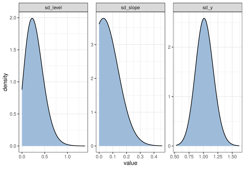
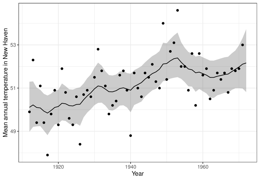
Figure 1 shows the estimated posterior densities of the three standard deviation parameters of the model. The relatively large observational level standard deviation suggests that the underlying latent temperature series is much smoother than the observed series, which can also be seen from Figure 2 which show the original observations (black dots) spread around the estimated temperature series (solid line).
library("dplyr")d <- as.data.frame(mcmc_bsm, variable = "states")summary_y <- d %>% filter(variable == "level") %>% group_by(time) %>% summarise(mean = mean(value), lwr = quantile(value, 0.025), upr = quantile(value, 0.975))ggplot(summary_y, aes(x = time, y = mean)) + geom_ribbon(aes(ymin = lwr, ymax = upr), alpha = 0.25) + geom_line() + geom_point(data = data.frame(mean = nhtemp, time = time(nhtemp))) + theme_bw() + xlab("Year") + ylab("Mean annual temperature in New Haven")
For non-Gaussian models the default MCMC algorithm is approximate inference based on Laplace approximation combined with importance sampling post-correction (Section Post-processing by importance weighting). It is also possible to perform first approximate MCMC using the argument mcmc_type = "approx", and then perform the post-correction step using the results from the approximate MCMC. In doing so, we can also use the function suggest_N to find a suitable number of particles for -APF in the spirit of Doucet et al. (2015):
out_approx <- run_mcmc(mng_model, mcmc_type = "approx", iter = 50000)est_N <- suggest_N(mng_model, out_approx)out_exact <- post_correct(mng_model, out_approx, particles = est_N$N)
The function suggest_N computes the standard deviation of the logarithm of the post-correction weights (i.e. the random part of log-likelihood of -APF) at the approximate MAP estimator of using a range of and returns a list with component N which is the smallest number of particles where the standard deviation was less than one. For small and moderate problems typically 10-20 particles is enough.
Filtering and smoothing
The bssm also offers separate methods for performing (approximate) state filtering and smoothing which may be useful in some custom settings.
For LGSSM, methods kfilter and smoother perform Kalman filtering and smoothing. For non-Gaussian models with linear-Gaussian dynamics, approximate filtering and smoothing estimates can be obtained by calls to kfilter and smoother, in which case these functions first construct an approximating Gaussian model for which the Kalman filter/smoother is then applied. For non-linear models defined by nlg_ssm we can run approximate filtering using the extended Kalman filter with the function ekf, the unscented Kalman filter with the function ukf, or the iterated EKF (IEKF) by changing the argument iekf_iter of the ekf function. Function ekf_smoother can be used for smoothing based on EKF/IEKF.
For particle filtering the bssm package supports general bootstrap particle filter for all model classes of the bssm (function bootstrap_filter). For nlg_ssm, extended Kalman particle filtering (Van Der Merwe et al., 2001) is also supported (function ekpf_filter).
For particle smoothing, function particle_smoother with the smoothing based on BSF is available for all models. In addition, -APF (using argument method = "psi") is available for all models except of ssm_sde class. Currently, only filter-smoother approach (Kitagawa, 1996) for particle smoothing is supported.
Comparison of IS-MCMC and HMC
Vihola et al. (2020) compared the computational efficiency of delayed acceptance MCMC and importance sampling type MCMC approaches in various settings. Here we make a small experiment comparing the generic Hamiltonian Monte Carlo using the NUTS sampler (Hoffman and Gelman, 2014) with rstan, and IS-MCMC with bssm. Given that the bssm is specialized for state space models whereas Stan is a general purpose tool suitable for wider range of problems, it is to be expected that bssm performs better in terms of computational efficiency. The purpose of this experiment is to illustrate this fact, i.e., that there is still demand for specialized algorithms for various types of statistical models. For complete code of the experiment, see Appendix: Code for section Comparison of IS-MCMC and HMC.
We consider the case of a random walk with drift model with negative binomial observations and some known covariate , defined as
with zero-mean Gaussian noise term with unknown standard deviation . Based on this we simulate one realization of and with , , , , .
For the IS approach we use ng_bsm function for model building, with prior variances 100 and 0.01 for the initial states and . For hyperparameters, we used fairly uninformative half-Normal distribution with standard deviation 0.5 for and 0.1 for . We then ran the IS-MCMC algorithm with run_mcmc using a burn-in phase of length 10,000 and run 50,000 iterations after the burn-in, with 10 particles per SMC.
Using the same set up, we ran the MCMC with rstan using 15,000 iterations (with first 5000 used for warm-up). Note that in order to avoid sampling problems, it was necessary to tweak the default control parameters of the sampler (see Appendix).
Table 1 shows the results. We see both methods produce identical results (within the Monte Carlo error), but while rstan produces similar Monte Carlo standard errors with smaller amount of total iterations than bssm, the total computation time of rstan is almost 80 times higher than with bssm (58 minutes versus 45 seconds), which suggests that for these type of problems it is highly beneficial to take advantage of the known model structure and available approximations versus general Bayesian software such as Stan which makes no distinction between latent states and hyperparameters .
| bssm | rstan | |||||
|---|---|---|---|---|---|---|
| Mean | SD | MCSE | Mean | SD | MCSE | |
Conclusions
State space models are a flexible tool for analysing a variety of time series data. Here we introduced the R package bssm for fully Bayesian state space modelling for a large class of models with several alternative MCMC sampling strategies. All computationally intensive parts of the package are implemented with C++ with parallel computation support for IS-MCMC making it an attractive option for many common models where relatively accurate Gaussian approximations are available.
Compared to early versions of the bssm package, the option to define R functions for model updating and prior evaluation have lowered the bar for analysing custom models. The package is also written in a way that it is relatively easy to extend to new model types similar to current bsm_lg in future. The bssm package could be expanded to allow other proposal adaptation schemes such as adaptive Metropolis algorithm by Haario et al. (2001), as well as support for multivariate SDE models and automatic differentiation for EKF-type algorithms.
Acknowledgements
This work has been supported by the Academy of Finland research grants 284513, 312605, 315619, 311877, and 331817.
References
- Andrieu et al. (2010) C. Andrieu, A. Doucet, and R. Holenstein. Particle Markov chain Monte Carlo methods. Journal of Royal Statistical Society B, 72(3):269–342, 2010.
- Banterle et al. (2019) M. Banterle, C. Grazian, A. Lee, and C. P. Robert. Accelerating Metropolis-Hastings algorithms by delayed acceptance. Foundations of Data Science, 1(2):103, 2019. URL https://doi.org/10.3934/fods.2019005.
- Carpenter et al. (2017) B. Carpenter, A. Gelman, M. Hoffman, D. Lee, B. Goodrich, M. Betancourt, M. Brubaker, J. Guo, P. Li, and A. Riddell. Stan: A probabilistic programming language. Journal of Statistical Software, 76(1):1–32, 2017. URL https://doi.org/10.18637/jss.v076.i01.
- Christen and Fox (2005) J. A. Christen and C. Fox. Markov chain Monte Carlo using an approximation. Journal of Computational and Graphical Statistics, 14(4):795–810, 2005. doi: 10.1198/106186005X76983. URL https://doi.org/10.1198/106186005X76983.
- de Valpine et al. (2017) P. de Valpine, D. Turek, C. Paciorek, C. Anderson-Bergman, D. Temple Lang, and R. Bodik. Programming with models: writing statistical algorithms for general model structures with NIMBLE. Journal of Computational and Graphical Statistics, 26:403–413, 2017. doi: 10.1080/10618600.2016.1172487.
- Doucet et al. (2015) A. Doucet, M. K. Pitt, G. Deligiannidis, and R. Kohn. Efficient implementation of Markov chain Monte Carlo when using an unbiased likelihood estimator. Biometrika, 102(2):295–313, 03 2015. ISSN 0006-3444. URL https://doi.org/10.1093/biomet/asu075.
- Durbin and Koopman (2000) J. Durbin and S. J. Koopman. Time series analysis of non-Gaussian observations based on state space models from both classical and Bayesian perspectives. Journal of Royal Statistical Society B, 62:3–56, 2000.
- Durbin and Koopman (2002) J. Durbin and S. J. Koopman. A simple and efficient simulation smoother for state space time series analysis. Biometrika, 89:603–615, 2002.
- Durbin and Koopman (2012) J. Durbin and S. J. Koopman. Time Series Analysis by State Space Methods. Oxford University Press, New York, 2nd edition, 2012.
- Eddelbuettel and François (2011) D. Eddelbuettel and R. François. Rcpp: Seamless R and C++ integration. Journal of Statistical Software, 40(8):1–18, 2011. URL https://doi.org/10.18637/jss.v040.i08.
- Eddelbuettel and Sanderson (2014) D. Eddelbuettel and C. Sanderson. Rcpparmadillo: Accelerating r with high-performance c++ linear algebra. Computational Statistics and Data Analysis, 71:1054–1063, March 2014. URL http://doi.org/10.1016/j.csda.2013.02.005.
- Franks and Vihola (2020) J. Franks and M. Vihola. Importance sampling correction versus standard averages of reversible MCMCs in terms of the asymptotic variance. Stochastic Processes and their Applications, 130(10):6157 – 6183, 2020. ISSN 0304-4149. URL http://www.sciencedirect.com/science/article/pii/S0304414919304053.
- Funk and King (2020) S. Funk and A. A. King. Choices and trade-offs in inference with infectious disease models. Epidemics, 30:100383, 2020. ISSN 1755-4365. URL https://doi.org/10.1016/j.epidem.2019.100383.
- Gordon et al. (1993) N. J. Gordon, D. J. Salmond, and A. F. M. Smith. Novel approach to nonlinear/non-Gaussian Bayesian state estimation. IEE Proceedings-F, 140(2):107–113, 1993.
- Haario et al. (2001) H. Haario, E. Saksman, and J. Tamminen. An adaptive metropolis algorithm. Bernoulli, 7(2):223–242, 04 2001. URL https://projecteuclid.org:443/euclid.bj/1080222083.
- Harvey (1989) A. C. Harvey. Forecasting, Structural Time Series Models and the Kalman Filter. Cambridge University Press, 1989.
- Helske (2016) J. Helske. ramcmc: Robust Adaptive Metropolis Algorithm, 2016. URL https://CRAN.R-project.org/package=ramcmc. R package version 0.1.0-1.1.
- Helske (2017) J. Helske. KFAS: Exponential family state space models in R. Journal of Statistical Software, 78(10):1–39, 2017. URL https://doi.org/10.18637/jss.v078.i10.
- Helske and Helske (2019) S. Helske and J. Helske. Mixture hidden Markov models for sequence data: The seqHMM package in R. Journal of Statistical Software, 88(3):1–32, 2019. URL https://doi.org/10.18637/jss.v088.i03.
- Hoffman and Gelman (2014) M. D. Hoffman and A. Gelman. The no-U-turn sampler: Adaptively setting path lengths in Hamiltonian Monte Carlo. The Journal of Machine Learning Research, 15(1):1593–1623, 2014.
- Iacus (2016) S. M. Iacus. sde: Simulation and Inference for Stochastic Differential Equations, 2016. URL https://CRAN.R-project.org/package=sde. R package version 2.0.15.
- Jacob and Funk (2020) P. E. Jacob and S. Funk. rbi: Interface to LibBi, 2020. URL https://CRAN.R-project.org/package=rbi. R package version 0.10.3.
- Jazwinski (1970) A. Jazwinski. Stochastic Processes and Filtering Theory. Academic Press, 1970.
- King et al. (2016) A. A. King, D. Nguyen, and E. L. Ionides. Statistical inference for partially observed Markov processes via the R package pomp. Journal of Statistical Software, 69(12):1–43, 2016. URL https://doi.org/10.18637/jss.v069.i12.
- Kitagawa (1996) G. Kitagawa. Monte Carlo filter and smoother for non-Gaussian nonlinear state space models. Journal of Computational and Graphical Statistics, 5(1):1–25, 1996.
- Lindgren and Rue (2015) F. Lindgren and H. Rue. Bayesian spatial modelling with R-INLA. Journal of Statistical Software, 63(19):1–25, 2015. URL https://doi.org/10.18637/jss.v063.i19.
- Michaud et al. (2020) N. Michaud, P. de Valpine, D. Turek, C. Paciorek, and D. Nguyen. Sequential Monte Carlo methods in the nimble R package. Technical Report arxiv:1703.06206, arXiv preprint, 2020.
- Murray (2015) L. Murray. Bayesian state-space modelling on high-performance hardware using LibBi. Journal of Statistical Software, Articles, 67(10):1–36, 2015. ISSN 1548-7660. URL https://doi.org/10.18637/jss.v067.i10.
- NIMBLE Development Team (2020) NIMBLE Development Team. nimbleSMC: Sequential Monte Carlo methods for NIMBLE, 2020. URL https://cran.r-project.org/package=nimbleSMC. R package version 0.10.0.
- Petris and Petrone (2011) G. Petris and S. Petrone. State space models in r. Journal of Statistical Software, 41(4):1–25, 2011. URL https://doi.org/10.18637/jss.v041.i04.
- Plummer et al. (2006) M. Plummer, N. Best, K. Cowles, and K. Vines. CODA: Convergence diagnosis and output analysis for MCMC. R News, 6(1):7–11, 2006. URL https://CRAN.R-project.org/doc/Rnews/.
- Stan Development Team (2020) Stan Development Team. RStan: the R interface to Stan, 2020. URL http://mc-stan.org/. R package version 2.21.2.
- Tusell (2011) F. Tusell. Kalman filtering in R. Journal of Statistical Software, 39(2):1–27, 2011. URL https://doi.org/10.18637/jss.v039.i02.
- Van Der Merwe et al. (2001) R. Van Der Merwe, A. Doucet, N. De Freitas, and E. A. Wan. The unscented particle filter. In Advances in neural information processing systems, pages 584–590, 2001.
- Vihola (2012) M. Vihola. Robust adaptive Metropolis algorithm with coerced acceptance rate. Statistics and Computing, 22(5):997–1008, 2012. ISSN 1573-1375. URL https://doi.org/10.1007/s11222-011-9269-5.
- Vihola et al. (2020) M. Vihola, J. Helske, and J. Franks. Importance sampling type estimators based on approximate marginal MCMC. Scandinavian Journal of Statistics, 2020. URL https://doi.org/10.1111/sjos.12492.
- Wickham (2016) H. Wickham. ggplot2: Elegant Graphics for Data Analysis. Springer-Verlag New York, 2016. ISBN 978-3-319-24277-4. URL https://ggplot2.tidyverse.org.
Appendix: Code for section Comparison of IS-MCMC and HMC
library("bssm")# Simulate the dataset.seed(123)n <- 200sd_level <- 0.1drift <- 0.01beta <- -0.9phi <- 5level <- cumsum(c(5, drift + rnorm(n - 1, sd = sd_level)))x <- 3 + (1:n) * drift + sin(1:n + runif(n, -1, 1))y <- rnbinom(n, size = phi, mu = exp(beta * x + level))# Construct model for bssmbssm_model <- bsm_ng(y, xreg = x, beta = normal(0, 0, 10), phi = halfnormal(1, 10), sd_level = halfnormal(0.1, 1), sd_slope = halfnormal(0.01, 0.1), a1 = c(0, 0), P1 = diag(c(10, 0.1)^2), distribution = "negative binomial")# run the MCMCfit_bssm <- run_mcmc(bssm_model, iter = 60000, burnin = 10000, particles = 10, seed = 1)# create the Stan modellibrary("rstan")stan_model <- "data { int<lower=0> n; // number of data points int<lower=0> y[n]; // time series vector[n] x; // covariate}parameters { real<lower=0> sd_slope; real<lower=0> sd_level; real beta; real<lower=0> phi; // instead of working directly with true state variables // it is often suggested use standard normal variables in sampling // and reconstruct the true parameters in transformed parameters block // this should make sampling more efficient although coding the model // is less intuitive. vector[n] level_std; // N(0, 1) level noise vector[n] slope_std; // N(0, 1) slope noise}transformed parameters { vector[n] level; vector[n] slope; // construct the actual states level[1] = 10 * level_std[1]; slope[1] = 0.1 * slope_std[1]; slope[2:n] = slope[1] + cumulative_sum(sd_slope * slope_std[2:n]); level[2:n] = level[1] + cumulative_sum(slope[1:(n-1)]) + cumulative_sum(sd_level * level_std[2:n]);}model { beta ~ normal(0, 10); phi ~ normal(0, 10); sd_slope ~ normal(0, 0.1); sd_level ~ std_normal(); // standardised noise terms level_std ~ std_normal(); slope_std ~ std_normal(); y ~ neg_binomial_2_log(level + beta * x, phi);}"stan_data <- list(n = n, y = y, x = x)stan_inits <- list(list(sd_level = 0.1, sd_slope = 0.01, phi = 1, beta = 0))# need to increase adapt_delta and max_treedepth in order to avoid divergencesfit_stan <- stan(model_code = stan_model, data = stan_data, iter = 15000, warmup = 5000, control = list(adapt_delta = 0.99, max_treedepth = 12), init = stan_inits, chains = 1, refresh = 0, seed = 1)d_stan <- summary(fit_stan, pars = c("sd_level", "sd_slope", "phi", "beta", "level[200]", "slope[200]" ))$summary[,c("mean", "sd", "se_mean")]d_bssm <- summary(fit_bssm, variable = "both", return_se = TRUE)# Parameter estimates:d_stand_bssm$thetad_bssm$states$Mean[200,]d_bssm$states$SD[200,]d_bssm$states$SE[200,]# Timings:sum(get_elapsed_time(fit_stan))fit_bssm$time[3]
Jouni Helske
Department of Mathematics and Statistics
University of Jyväskylä
Finland
ORCiD: 0000-0001-7130-793X
jouni.helske@jyu.fi
Matti Vihola
Department of Mathematics and Statistics
University of Jyväskylä
Finland
ORCiD: 0000-0002-8041-7222
matti.s.vihola@jyu.fi