The impact of limited time resolution on the
forward-scattering polarization
in the solar Sr I 4607 Å line
Abstract
Theoretical investigations predicted that high spatio-temporal resolution observations in the Sr I 4607 Å line must show a conspicuous scattering polarization pattern at the solar disk-center, which encodes information on the unresolved magnetism of the inter-granular photospheric plasma. Here we present a study of the impact of limited time resolution on the observability of such forward scattering (disk-center) polarization signals. Our investigation is based on three-dimensional radiative transfer calculations in a time-dependent magneto-convection model of the quiet solar photosphere, taking into account anisotropic radiation pumping and the Hanle effect. This type of radiative transfer simulation is computationally costly, reason why the time variation had not been investigated before for this spectral line. We compare our theoretical results with recent disk-center filter polarimetric observations in the Sr I 4607 Å line, showing that there is good agreement in the polarization patterns. We also show what we can expect to observe with the Visible Spectro-Polarimeter at the upcoming Daniel K. Inouye Solar Telescope.
Subject headings:
Polarization - scattering - radiative transfer - Sun: photosphere - Sun: magnetism1. Introduction
Even the quietest regions of the solar atmosphere are permeated by magnetic activity, happening at scales smaller than what we have been able to historically resolve. Recent investigations indicate that the magnetic energy density stored at these scales is so significant that this small-scale magnetism could potentially be the main driver for heating the outer layers of the solar atmosphere above the quiet regions of the solar disk (Trujillo Bueno et al. 2004; Amari et al. 2015; Rempel 2017).
The radiation field within the solar atmosphere is anisotropic because there is an unbalance between the radiation traveling upwards and sideways. As a result, the radiatively-induced transitions produce atomic level polarization, which in turns produces the so-called scattering line polarization. This occurs even in the absence of magnetic fields. If the intensity of the pumping radiation had axial symmetry around the local vertical, the only source of scattering polarization at the solar disk-center would be the presence of a non-vertical magnetic field (Trujillo Bueno, 2001; Landi Degl’Innocenti & Landolfi, 2004). However, the situation in the Sun is more interesting, as both the horizontal inhomogeneities and velocity gradients break the axial symmetry of the incident radiation field, producing scattering polarization at disk-center even in the absence of magnetic fields (e.g., Manso Sainz & Trujillo Bueno 2011; Štěpán & Trujillo Bueno 2016). Therefore, with some exceptions (e.g., Trujillo Bueno et al. 2002), the observation of forward scattering polarization is not indicative of magnetic activity by itself. However, the degree and angle of this polarization greatly depends on the magnetic field vector in the region of formation of the spectral line under consideration.
One spectral line of especial interest to study the small-scale magnetic activity in the quiet regions of the solar photosphere is the Sr I transition at 4607 Å , because it shows polarization amplitudes among the largest in the second solar spectrum (Stenflo et al. 1997; Gandorfer 2002), its scattering polarization is sensitive to magnetic field strengths as large as 300 G, and because its polarization can be reliably calculated using a two-level atomic model. In 2004, advanced theoretical modeling of spectropolarimetric data for this spectral line led to the discovery of a vast amount of hidden magnetic energy in the quiet Sun, due to the presence of a small-scale magnetic field with a mean field strength of the order of G (Trujillo Bueno et al. 2004), concluding that the statistical properties of the photospheric magnetic field in the quiet-Sun inter-network regions vary at the spatial scales of the solar granulation pattern.
Recently, del Pino Alemán et al. (2018) solved the radiation transfer problem of scattering polarization in the Sr I 4607 Å line using a high-resolution three-dimensional (3D) model resulting from advanced magneto-convection simulations (Rempel, 2014). The selected snapshot model has a mean field strength of G at the model’s visible surface and a convection zone magnetized close to the equipartition. They demonstrated that the magnetic field of the model’s photosphere produces a Hanle depolarization compatible with scattering polarization observations of the Sr I 4607 Å line without spatio-temporal resolution. The authors continued and expanded the investigation of Trujillo Bueno & Shchukina (2007) providing useful information to facilitate high spatio-temporal resolution observational advances, in particular the detection of the theoretically-predicted disk-center polarization patterns.
Motivated by the theoretical investigation of Trujillo Bueno & Shchukina (2007), observations with the Zürich Imaging Polarimeter (ZIMPOL) have been carried out at the GREGOR telescope of the Observatorio del Teide (Tenerife; Spain) to study the spatial variability of the polarization signals at different distances from the solar limb (Bianda et al. 2018; Dhara et al. 2019), finding variations at granular scales for all the observed heliocentric angles. More recently, Zeuner et al. (2020) used the Fast Solar Polarimeter (FSP 2) attached to the Dunn Solar Telescope of the Sacramento Peak Observatory (USA) and applied a novel strategy to increase the signal to noise ratio of their disk-center filter polarimetric observations in the Sr I 4607 Å line. Although their successful detection of forward scattering polarization confirms the theoretical predictions, a satisfactory confrontation with the recent theoretical results of del Pino Alemán et al. (2018) requires taking into account the instrumental degradation produced by their specific observational setup.
The solution of the radiative transfer problem of scattering polarization in 3D models of the solar atmosphere is very computationally intensive. For this reason, the previous investigations used a single snapshot from a hydrodynamical or magneto-hydrodynamical simulation, neglecting the impact on the polarization signals due to the limited temporal resolution. In this work we extend our previous study (del Pino Alemán et al. 2018) by including the effect of the temporal evolution on the observed scattering polarization in a 3D time-dependent model of the solar photosphere. To this end, we have solved the aforementioned radiative transfer problem in 151 3D snapshots of a magneto-convection simulation covering five minutes of solar time. In section §2 we summarize the properties of the time series we use and the synthesis method. In section §3 we study the effect of the limited time resolution on the emergent Stokes profiles. Finally, in section §4 we study the joint effect of the limited time resolution and the instrumental effects for two observational setups of interest: the filter polarimeter used by Zeuner et al. (2020) and the (slit-based) Visible Spectro-Polarimeter (ViSP) attached to the Daniel K. Inouye Solar Telescope (DKIST).
2. The Physical Problem
The 3D model of the quiet solar photosphere used in this investigation is a time series of a magneto-convection simulation by Rempel (2014). The original grid of the 3D snapshots has points, with a regular spacing of km in the three dimensions. For our calculations, we have cut the magneto-hydrodynamical (MHD) model in the vertical direction in order to include only the region of the atmosphere that is relevant for the formation of the Sr I 4607 Å line. The atmospheric model we use in our calculations thus has grid points, with the vertical axis going from km below to km above the average height where the optical depth of the continuum at 4607 Å is unity, and the same km grid resolution. The simulation had a fixed time step of s, storing one every ten time steps; therefore, the snapshots have a cadence of s.
The calculations of the emergent Stokes profiles have been carried out as in del Pino Alemán et al. (2018), with the radiative transfer code PORTA (see Štěpán & Trujillo Bueno, 2013)222PORTA is publicly available at https://gitlab.com/polmag/PORTA, which solves the non-LTE multilevel problem of the generation and transfer of polarized radiation in 3D Cartesian models of stellar atmospheres taking fully into account the breaking of the axial symmetry of the incident radiation field at each point within the medium.
We first solved the problem of the strontium ionization balance in order to obtain the number density of strontium atoms in the lower and upper levels of the Sr I line at 4607 Å at each spatial point of the 3D model. To this end, we used the same 15 levels atomic model and abundance than in del Pino Alemán et al. (2018) and the same numerical code than in del Pino Alemán et al. (2020). We then used a two-level atomic model to compute with PORTA the Stokes profiles of the Sr I 4607 Å line. For the rates of depolarizing collisions with neutral hydrogen atoms we have taken the expression given by Faurobert-Scholl et al. (1995).
In our 3D radiative transfer calculations of the scattering polarization in the Sr I 4607 Å line we do not include the polarization of the continuum radiation caused by Rayleigh and Thomson scattering (see Trujillo Bueno & Shchukina, 2009). This is a suitable approximation because at 4607 Å the continuum polarization amplitude is, in general, much smaller than that of the line itself.
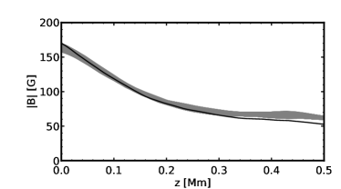
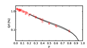
The time series studied in this paper ( km spatial resolution) is not the same one from where the snapshot used by del Pino Alemán et al. (2018) was extracted (8 km spatial resolution). The left panel in Fig. 1 shows the variation with height of the average magnetic field strength in all the km snapshots (gray curves) and in the km model used in del Pino Alemán et al. (2018) (black curve); they are very similar in the region of formation of the Sr I line at 4607 Å (approximately between 170 and 350 km above the visible continuum surface) and the 8 km one shows an average magnetic field strength within the range of variability of the time series. The right panel in Fig. 1 shows the CLV of the average fractional linear polarization in all the snapshots (gray curves) and in the single snapshot model used by del Pino Alemán et al. (2018) (black curve), while the red circles show various observations taken during a minimum and maximum of the solar activity cycle (see Trujillo Bueno et al. 2004). The CLV obtained from the high-resolution (8 km) single snapshot model (black curve) produces an excellent fit to the observations. The fit provided by the CLV obtained from the lower-resolution (16 km) time series models is also satisfactory, although it is not as extraordinary as that provided by the 8 km magneto-convection model. Note that, regardless of the small differences seen in Fig. 1, both CLV tend to zero at disk-center, as the plotted quantity lacks any spatial resolution. In summary, the time series snapshot models resulting from Rempel’s (2014) 16 km resolution magneto-convection simulations are fully appropriate for this investigation and, in particular, for investigating the relative impact of the time resolution on the scattering polarization.
3. The Effect of Time Resolution
In this section we study the effect that a limited time resolution has on the spatial pattern and amplitudes of the linear polarization signals for observations at the disk-center. The solar atmosphere is continuously evolving, so it varies during the exposure time of our observations. Because the polarization is a signed quantity, it is significantly more affected by this evolution than the intensity. We are interested, in particular, on how the exposure time affects the mean amplitude of the line center polarization of our synthetic profiles, as well as the effect on the fine spatial structure and fluctuation pattern.
In order to study this effect, we integrate the Stokes parameters for each wavelength and for each point in the field of view among a number of snapshots covering different exposure times. Figure 2 shows the intensity and the fractional linear polarization at the line center for the disk-center line of sight, for the first snapshot of the time series and for different exposure times; from left to right and top to bottom, instantaneous, s, s, s, s, and s. As expected, the impact of the exposure time on the scattering polarization is apparent, at plot level, for smaller times than for the intensity. The intensity is blurred and gradually loses contrast, very noticeable especially in the bottom row of the intensity panels in Fig. 2 (integration time s). Regarding the fractional linear polarization , the loose of details is already easily seen for s, and the decrease of contrast is more apparent due to the signed nature of the polarization. Notice that, while in most of the field of view the time integration results in decreasing signals (see green arrow in Fig. 2 for an example) there are some regions where the polarization increases as a result of the time evolution of the granulation pattern (e.g., red arrow in Fig. 2).
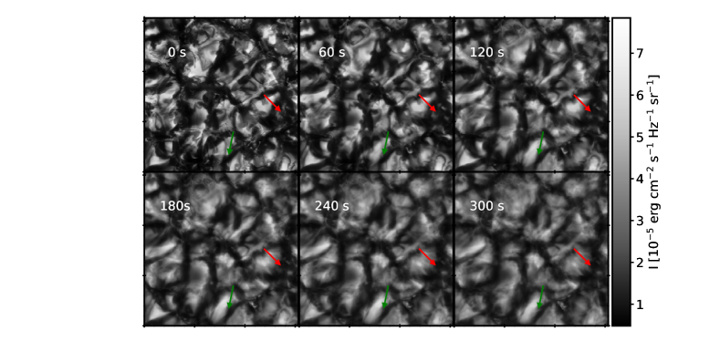
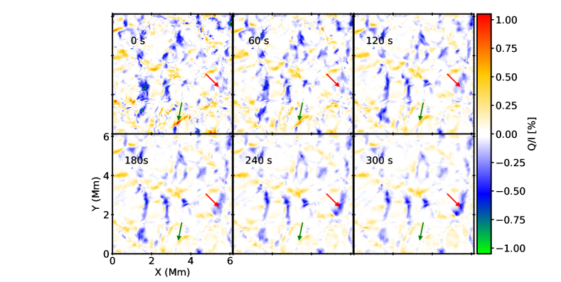
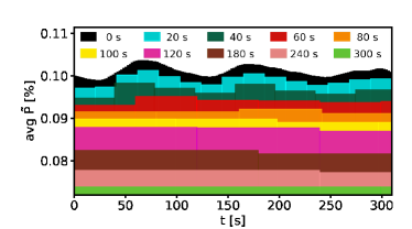
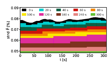
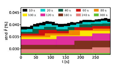
Figure 3 shows the time evolution of the mean value and the standard deviation of the total linear polarization in the time series after integrating for different exposure times (see legend in the figure). The chosen average is given by
| (1) |
with the average intensity value, in time and space, of the whole series, used for all time steps and integration times. All Stokes parameters are taken at line center, for the disk-center line of sight. We have chosen this polarization quantity because it is unsigned; that is, the mean value of the individual and signals is clearly affected by sign cancellation, but is not. Additionally, the standard deviation of , , and show the same behavior.
Without taking into account any other instrumental effects besides the limited time resolution, the average value and standard deviation of the total linear polarization is already reduced % for one minute of exposure time; that is, even a perfect instrument without any degradation of the spatial resolution cannot fully detect the instantaneous polarization signals due to the finite exposure time.
4. Instrumental Effects
In this section we study the effect on the intensity and linear polarization of the Sr I 4607 Å line caused by the plasma evolution during the finite exposure time (section §3), but including now the instrumental effects (see del Pino Alemán et al. 2018 for an analysis of instrumental effects without the impact of time evolution for the same spectral line). We consider two relevant instrumental setups: a filter polarimeter and a slit-based spectropolarimeter.
4.1. Filter polarimeter
This instrumental setup is of particular interest because it is similar to that used by Zeuner et al. (2020). Although they could not directly observe the linear polarization pattern predicted by our disk-center simulations (Fig. 2), they were able to detect the expected linear polarization signals after applying a novel analysis technique. We want to test what happens to the time series simulation when we mimic the degradation produced by a Fabry–Pérot instrument similar to theirs. Our degradation steps are the following:
-
•
Telescope of 0.76 m diameter and ” spatial resolution ( m), computed with the long exposure MTF from Fried (1966).
-
•
Spatial sampling of 0.2”/pix (resulting from a 3x3 bining as in Zeuner et al. 2020)
-
•
Gaussian filter with 67 mÅ of full width at half maximum (FWHM). As in Zeuner et al. (2020), this filter is shifted 20 mÅ to the blue of the theoretical Sr I 4607 Å line center.
-
•
Noise in Stokes and from a normal distribution with (hereafter, 0.4 %) for each snapshot ( s exposure), which corresponds to approximately % for a min integration.
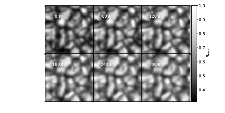
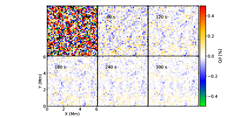
Once we degraded all the snapshots following these steps, we proceeded to integrate them in time to simulate different exposure times. Figure 4 shows the intensity and fractional linear polarization for the filter polarimeter described above. The intensity (top panels) has been normalized to the maximum for each panel. We note that the increase of integration time decreases the contrast (, from to between the first and last panel). For the polarization we have limited the plotting range of values to . This improves the visualization of most of the panels, but makes it so that the first panel is saturated. However, the first panel shows pure noise. We can see that a five minutes integration returns a pattern that reminds us of the original snapshot (see fig. 2), but the amplitude of the signal is decreased significantly.
However, a closer look into the details in the bottom panel of Fig. 4 shows that, even for a min integration, the resulting linear polarization is severely affected by the noise (see also the top panels in fig. 5, where we have saturated the color scale for an easier visualization). It is also of interest to show the disk-center fractional linear polarization map that the filter polarimeter would observe if there were no noise (see bottom panel in Fig. 5). A comparison with the bottom panel in Fig. 2 shows that in the noise-free ideal case the instrumental setup used by Zeuner et al. (2020) would reduce the original theoretical polarization amplitudes by more than an order of magnitude, but would keep the structure of the predicted polarization pattern. However, as seen in the top panel of Fig. 5, the noise level is such that this pattern is almost lost even for a five minutes integration time.
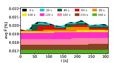
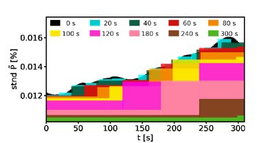
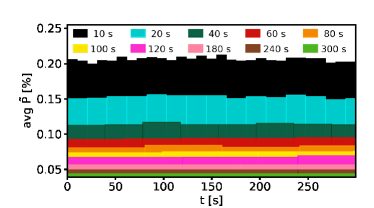
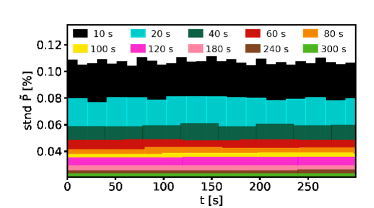
Regarding the time evolution of the mean value and the standard deviation of the total linear polarization in the degraded time series, for different exposure times (see Fig. 6) we see that the effect of the noise is critical for the statistics of the observation. In the noise-free case (top panels), we see some time evolution (notice, however, that the range of variation in the figure is very small, namely, 0.004 %) and mean and standard deviation values much smaller than in the original simulation (fig. 3). This decrease is a consequence of the simulated instrumental effects. However, when noise is included it dominates the time evolution and the statistics, especially for small integration times. For this reason, both the mean and standard deviation quickly decrease with the integration time when the noise is taken into consideration (see the bottom panels of Fig. 6).
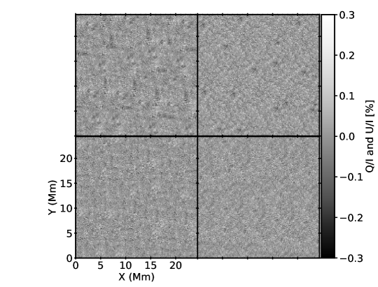
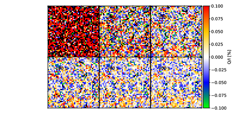
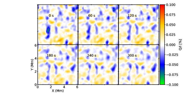
In order to compare with the observations by Zeuner et al. (2020) we show the case of s exposure time in the same amplitude and color scale used by them (see bottom panels in Fig. 7). To study the effect of the time evolution on the polarization amplitudes, we have taken the initial snapshot applying to it the same degradation procedure, but with a polarization noise with % (the equivalent value for a s integration). In order to present a field of view similar to the one of their observation, we have replicated 16 times the field of view of the model’s snapshots; however, we have introduced some shifts between the pieces of the mosaic to avoid the obvious pattern repetition that we would have if we just replicated the same plane. It seems, from visual comparison with Zeuner et al. (2020), that we get slightly larger polarization amplitudes than in their observation, consistent with their finding regarding the noise distribution difference between and explained in appendix B of Zeuner et al. (2020). Moreover, although there are some differences between the top and bottom panels in Fig. 7, we can see that taking into account the exposure time of their s observation does not dramatically impact the average amplitude (as suggested by the noise-free average in the top left panel of Fig. 6). However, the amplitude is dominated by noise (see Fig. 5). Note that, even though we have assumed a duty cycle of 100 % when integrating the different snapshots, the comparison with Zeuner et al. (2020) is still valid because the FSP 2 has a duty cycle of 98 % (Iglesias et al., 2016).
4.2. Slit-based spectropolarimeter
Our second instrumental setup is the Visible Spectro-Polarimeter (ViSP) at the DKIST (e.g., Elmore et al. 2014). We have chosen this slit-based spectropolarimeter because it is of present interest to predict what type of scattering polarization signals we can expect to observe using the ViSP at the world’s largest solar telescope. Our degradation steps are the following:
-
•
Telescope of 4 m diameter and ” spatial resolution ( m) computed with the long exposure MTF from Fried (1966). Clearly, such spatial resolution requires the use of adaptive optics.
-
•
Spectral point spread function, convolution with a gaussian with 33.69 mÅ FWHM.
-
•
Spectrograph slit with a ” width (this results in ” spatial resolution in the scanning direction).
-
•
Spectral sampling of 34 mÅ /pixel and spatial sampling along the slit of ”/pixel.
-
•
Noise in Stokes and from a normal distribution with % (relative to the continuum intensity) for each snapshot ( s exposure), which corresponds to a signal to noise ratio (SNR) of .
The numerical values for the ViSP degradation have been obtained using the ViSP IPC333https://www.nso.edu/telescopes/dkist/instruments/visp/, a calculator for observation planning.
Once we degraded all the snapshots following these steps, we proceeded to integrate them in time to simulate different exposure times. In the present ViSP slit spectropolarimeter case we have simulated the scan, i.e., the exposure time corresponds to the time each slit is kept in position. Because scanning a field of view of this size (”) with this slit width and step (we move the slit a distance equal to its width, ”) requires more than five minutes for reasonable exposure times, we quickly run out of snapshots to integrate. To solve this, whenever we reach the end of the series, we switch the direction of the time evolution, that is, the time series mirrors itself whenever it reaches the last snapshot. Note, however, that we do not take into account other effects such as the possible misalignments and the finite time in the scan that should be devoted to the reading of the cameras or the movement of the slit.
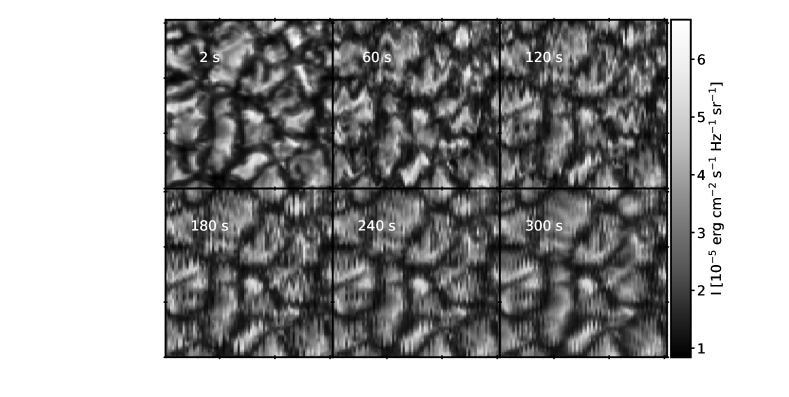
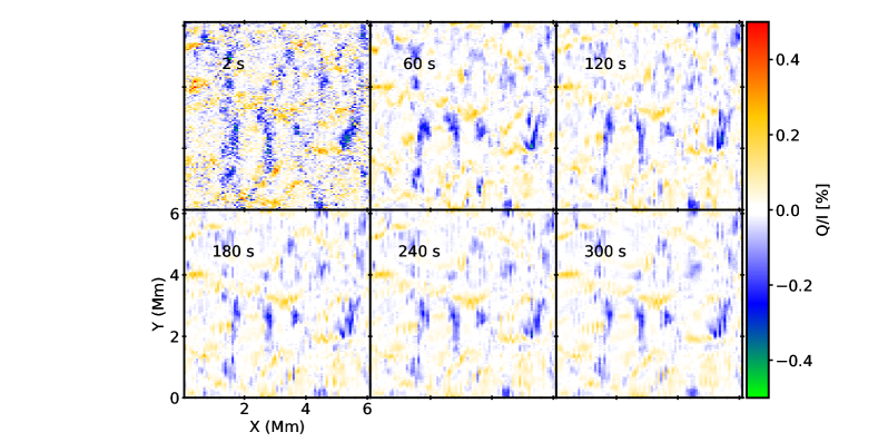
Figure 8 shows the intensity and fractional linear polarization for the slit spectropolarimeter described above. As it happened with the filter polarimeter, larger integration times result in a decreased intensity contrast (from to between the first and last Stokes panel). We can also see the effect of the scanning in the reconstructed image when we increase the integration time. This effect is, in fact, underestimated, as our time series is roughly five minutes long and we have repeated it as many times as necessary to cover the whole simulation field of view with the chosen slit. If we had a long enough series, the difference in the granulation pattern between the reconstructed intensity and the result of the simulation would be more significant. On the other hand, the much higher SNR for the m telescope is very apparent, as only in the instantaneous snapshots can we clearly see the noise, greatly diminished already after a s integration. Notice that even with this relatively high spatial resolution (””) the simulated signal is roughly a factor smaller than the one obtained in the simulation.
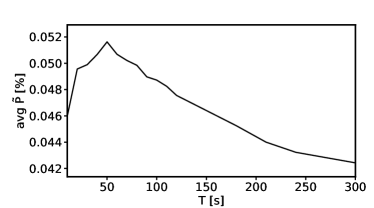
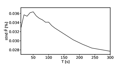
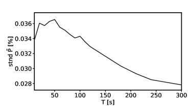
Figure 9 shows the variation of the mean value and the standard deviation of (Eq. (1)) for different integration times. Because with this instrumental setup we need to scan along one of the spatial directions, there is no time evolution. The initial rise on the statistics can be due to their temporal evolution, as both the mean and standard deviation increase during the first s in the synthetic maps (see Fig. 3). After this initial increase, the curves are dominated by the time integration and both the average and standard deviation values decay resembling an order three polynomial. Because this setup simulates a m telescope working at ” resolution, the SNR is much higher and the impact of the noise is much smaller than with the filter polarimeter setup (compare top and bottoms panels in Fig. 9).
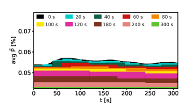
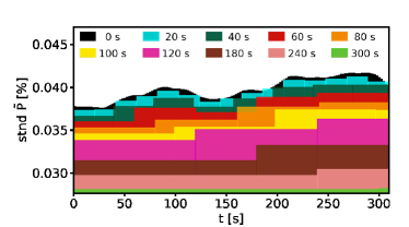
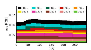
For the sake of comparison, we have also computed the variation of the mean and the standard deviation with time for different integration times assuming that for each observation we can cover the whole field of view simultaneously with the necessary number of slits (hereafter, the multiple-slit spectropolarimeter case; see Fig. 10). By comparing figures 3, 6, and 10, we can conclude that the impact of the time integration on the characteristics of the polarization signal, at least for the times relevant to the Sr I 4607 Å line, are rather reduced. The largest impact is found for the filter polarimeter case, but this is purely due to the smaller SNR of the case study, as ignoring the noise results in a similar decrease in the average and the standard deviation (see top panels in Fig. 6).
5. Concluding comments
We have solved the radiative transfer problem of scattering polarization in the Sr I 4607 Å line in a 3D magneto-convection time series model of the quiet solar photosphere. We studied the impact on the disk-center scattering polarization map due to the limited time resolution by integrating an increasing number of snapshots to simulate increasingly longer observing exposures.
As expected, taking into account the finite time resolution of spectropolarimetric observations in our theoretical results leads to a reduction of the average linear polarization signal, as well as to a decrease in the visibility of its spatial variability which we have characterized by means of the standard deviation.
We chose two instrumental setups of interest, a filter polarimeter similar to that used by Zeuner et al. (2020) and the ViSP instrument at DKIST.
For integration times below the evolution time scale of the granulation ( min), we find that the linear polarization signals in the filter polarimeter setup are strongly affected by the noise, demonstrated by the remarkable agreement that can be found between the histograms of the linear polarization signals from our simulations and from the unreconstructed observations in Zeuner et al. (2020). If we instead compare our simulation without noise with the reconstruction in Zeuner et al. (2020), we can see that our theoretical forward scattering signals are larger by about a factor . However, we think that this difference is mainly due to the limitations of their denoising reconstruction method, and not so much to real intrinsic differences between the prediction and the observations. It is clear, however, that further observations with better signal to noise ratio are needed in order to fully demonstrate this.
We have also shown the type of interesting observations of the disk-center polarization signals of the Sr I 4607 Å line that we can expect from the ViSP instrument at the upcoming DKIST. We must emphasize that, due to the limited minutes duration of our time series, we underestimate the effect of the time evolution of the solar plasma when scanning the field of view, as we can only loop over the time series, reducing the variability of the granulation pattern.
In conclusion, our results do indicate that it will be worthwhile to use the DKIST to map the forward scattering polarization of the Sr I 4607 Å line to achieve the unprecedented spatio-temporal resolution expected for such 4 m aperture telescope. This should be attempted using both, a filter polarimeter having a FWHM significantly smaller than the one considered in this paper and the ViSP, but the ideal instrument would be a multi-slit spectropolarimeter capable of simultaneously observing a 2D field of view. The data that such near-future observations will provide will be very valuable to probe the unresolved magnetism of the inter-granular lanes via the Hanle effect.
References
- Amari et al. (2015) Amari, T., Luciani, J.-F., & Aly, J.-J. 2015, Nature, 522, 188
- Bianda et al. (2018) Bianda, M., Berdyugina, S., Gisler, D., et al. 2018, ArXiv e-prints
- del Pino Alemán et al. (2020) del Pino Alemán, T., Trujillo Bueno, J., Casini, R., & Manso Sainz, R. 2020, ApJ, 891, 91
- del Pino Alemán et al. (2018) del Pino Alemán, T., Trujillo Bueno, J., Štěpán, J., & Shchukina, N. 2018, ApJ, 863, 164
- Dhara et al. (2019) Dhara, S. K., Capozzi, E., Gisler, D., et al. 2019, A&A, 630, A67
- Elmore et al. (2014) Elmore, D. F., Rimmele, T., Casini, R., et al. 2014, in Society of Photo-Optical Instrumentation Engineers (SPIE) Conference Series, Vol. 9147, Ground-based and Airborne Instrumentation for Astronomy V (Proc SPIE), 914707
- Faurobert-Scholl et al. (1995) Faurobert-Scholl, M., Feautrier, N., Machefert, F., Petrovay, K., & Spielfiedel, A. 1995, A&A, 298, 289
- Fried (1966) Fried, D. L. 1966, Journal of the Optical Society of America (1917-1983), 56, 1372
- Gandorfer (2002) Gandorfer, A. 2002, The Second Solar Spectrum: A high spectral resolution polarimetric survey of scattering polarization at the solar limb in graphical representation. Volume II: 3910 Å to 4630 Å
- Iglesias et al. (2016) Iglesias, F. A., Feller, A., Nagaraju, K., & Solanki, S. K. 2016, A&A, 590, A89
- Landi Degl’Innocenti & Landolfi (2004) Landi Degl’Innocenti, E., & Landolfi, M. 2004, Polarization in Spectral Lines (Kluwer Academic Publishers)
- Manso Sainz & Trujillo Bueno (2011) Manso Sainz, R., & Trujillo Bueno, J. 2011, ApJ, 743, 12
- Rempel (2014) Rempel, M. 2014, ApJ, 789, 132
- Rempel (2017) —. 2017, ApJ, 834, 10
- Stenflo et al. (1997) Stenflo, J. O., Bianda, M., Keller, C. U., & Solanki, S. K. 1997, A&A, 322, 985
- Trujillo Bueno (2001) Trujillo Bueno, J. 2001, in Astronomical Society of the Pacific Conference Series, Vol. 236, Advanced Solar Polarimetry – Theory, Observation, and Instrumentation, ed. M. Sigwarth, 161
- Trujillo Bueno et al. (2002) Trujillo Bueno, J., Landi Degl’Innocenti, E., Collados, M., Merenda, L., & Manso Sainz, R. 2002, Nature, 415, 403
- Trujillo Bueno & Shchukina (2007) Trujillo Bueno, J., & Shchukina, N. 2007, ApJ, 664, L135
- Trujillo Bueno & Shchukina (2009) —. 2009, ApJ, 694, 1364
- Trujillo Bueno et al. (2004) Trujillo Bueno, J., Shchukina, N., & Asensio Ramos, A. 2004, Nature, 430, 326
- Štěpán & Trujillo Bueno (2013) Štěpán, J., & Trujillo Bueno, J. 2013, A&A, 557, A143
- Štěpán & Trujillo Bueno (2016) —. 2016, ApJ, 826, L10
- Zeuner et al. (2020) Zeuner, F., Manso Sainz, R., Feller, A., et al. 2020, The Astrophysical Journal, 893, L44