Simulation of the cosmic ray effects for the LiteBIRD satellite observing the CMB B-mode polarization

Abstract

The LiteBIRD satellite is planned to be launched by JAXA in the late 2020s. Its main purpose is to observe the large-scale B-mode polarization in the Cosmic Microwave Background (CMB) anticipated from the Inflation theory. LiteBIRD will observe the sky for three years at the second Lagrangian point (L2) of the Sun-Earth system. Planck was the predecessor for observing the CMB at L2, and the onboard High Frequency Instrument (HFI) suffered contamination by glitches caused by the cosmic-ray (CR) hits. We consider the CR hits can also be a serious source of the systematic uncertainty for LiteBIRD. Thus, we have started a comprehensive end-to-end simulation study to assess impact of the CR hits for the LiteBIRD detectors. Here, we describe procedures to make maps and power spectra from the simulated time-ordered data, and present initial results. Our initial estimate is that $C_{l}^{BB}$ by CR is $\sim 2\times 10^{-6}~{}\mu$K${}_{\mathrm{CMB}}^{2}$ in a one-year observation with 12 detectors assuming that the noise is 1 aW/$\sqrt{\mathrm{Hz}}$ for the differential mode of two detectors constituting a polarization pair.

1 INTRODUCTION

LiteBIRD is a satellite dedicated for observing the anisotropy of the linear polarization of the Cosmic Microwave Background (CMB). It aims to detect the B-mode signal at a large angular scale ($l<200$) with the sensitivity of the tensor-to-scalar ratio $\Delta r\leq 0.001$ for constraining the theory of inflation. LiteBIRD has three telescopes, (LFT, MFT, and HFT), covering 15 frequency bands over 34–448 GHz. At the focal plane of each telescope, thousands of Transition Edge Sensor (TES) bolometers are placed, cooled at 100 mK. LiteBIRD is planned to be launched in the late 2020s by JAXA and is currently under design by an international collaboration among many institutions in Europe, North America, and Japan. General descriptions can be found elsewhere[1, 2].

LiteBIRD will scan the entire sky for three years from the second Lagrange point (L2) of the Sun-Earth system. It is becoming a popular destination among astronomical satellites for providing a more thermally benign environment than near-Earth orbits. However, L2 is also known to provide a more harsh environment in terms of cosmic-ray (CR) radiation [3]. CRs at L2 mainly consist of the Galactic Cosmic Rays (GCR) and Solar Energetic Particles (SEP). GCR is a permanent component with a hard spectrum, while SEP is an eruptive component with a soft spectrum associated with solar flares. Two major effects are anticipated in response to CR radiation: total-dose effects (TDE) and single event effects (SEE). Here, we consider SEE to the detector caused by GCR. SEP events are eruptive and small in a fraction of time, thus the data can be discarded during events similarly to Planck HFI[3].

Previous satellites suffered impacts on scientific products caused by SEE of the detectors by GCR [4]. It will be more serious for future satellites with an increasingly high demand on instrument sensitivity. It is mandatory to assess the impact of the CRs based on simulation at an early stage of the mission before fixing the hardware design. This is currently underway for LiteBIRD. An early result is described in a series of two articles. One is by Stever et al.[5], which describes the overview of this study and covers the details of the simulation from the CR spectrum to the Time-Ordered Data (TOD) and predicted $\Delta r$. This article covers the details of the simulation from the TOD to sky maps and power spectrum.

We first start with a brief comparison with the Planck HFI (§ 2), which is the predecessor to LiteBIRD, to predict the CR effects of LiteBIRD. We describe our simulation in § 3 for the input data (§ 3.1) and the output products (§ 3.2). In § 4, we discuss its validity (§ 4.1) and scaleability (§ 4.2), and discuss implications obtained through this exercise. We conclude in § 5.

2 COMPARISON WITH PANCK HFI

The High Frequency Instrument (HFI)[6] on the Planck satellite[7] is the closest predecessor of LiteBIRD for observing the sky in the 100–857 GHz band over a large angular scale at L2 using low-temperature detectors cooled at 100 mK. HFI had 20 spider-web bolometers (SWB) sensitive to thermal intensity and 16 Polarization-Sensitive Bolometer pairs (PSB-a and PSB-b). The spider-like radio absorbers were designed to minimize the cross section to CRs[8] and the temperature rise by input energy was detected by NTD Germanium thermistors. Each detector was situated on its own Si wafer die and was sensitive only to a single frequency and a single linear polarization direction.

HFI achieved unprecedented sensitivity and demonstrated both the technical feasibility and the superb scientific performance of low-temperature detectors operating at L2 [9]. However, it also suffered contamination by CRs, which appeared as numerous glitches of a short rise and slow decay profile in the TOD. Through the studies of in-orbit data[7, 3] as well as ground testing[4], it was found that the glitches are classified into three populations characterized by different time scales and amplitudes, which were dubbed as short, long, and slow glitches. The long glitches were the most numerous population, which were caused by CR events hitting the Si die of the detector. The rapid propagation of thermal energy as ballistic (athermal) phonons played a role in heat conduction. Short glitches were less dominant, which were caused by CR events directly impacting the absorbers and thermisters. Slow glitches were least frequent, which were considered to originate from the part unique to PSB-a, as the population was only found in PSB-a. Eventually, these glitches were removed by subtracting a template of each population in the time domain during the ground pipeline processing.

Accounting on some major design differences between LiteBIRD and Planck HFI, we can predict the impact to some extent. The first difference is the number of detector channels, in which the number increases by $\sim$10² times for LiteBIRD (Table 2). A single detector has multiple channels sensitive to different frequencies and directions of linear polarization. Many detectors are fabricated in a single common Si wafer (Fig. 1). A single CR hit on a wafer will impact all the detectors on the wafer, and cause common-mode noise among different frequency bands and between two polarization angles. As the wafer area and volume are much larger in LiteBIRD than Planck HFI, the event rate of the long glitches will be much higher but the amplitude will be smaller for a larger heat capacity. These may make the noise spectrum caused by long glitches behaves more like a Gaussian white noise.

Comparison of Planck HFI and LiteBIRD. For the wafer, LF-1 is used for LiteBIRD as a representative. Satellite/ Thermometer Si wafer Instrument Type $\tau$^a $f_{\mathrm{sample}}$^b Area^c $C$^d Det num^e Area^c Depth^f $C$^d (ms) (Hz) (mm²) (pJ/K) (cm²) (mm) (nJ/K) Plank / HFI NTD Ge 10 180 0.03 0.9 1 0.4-0.8 0.36 0.3 LiteBIRD TES 3 19 0.4 1.1 216 100 2.5 15

• Time constant of the detector, including thermo-electric feedback of a loop gain of 10 for TES.

• Downlink data rate per detector channel.

• Area of target. Surrounding parts included for LiteBIRD.

• Heat capacitance of target.

• Number of detector channels in a wafer excluding dark detectors.

• Depth of target.

The second difference is the data rate. Because of the increased number of detectors albeit a similar telemetry bandpass to the ground stations, the data rate per detector must be reduced for LiteBIRD to 19 Hz. In Planck HFI, the rate of 180 Hz for each detector allowed to resolve CR glitches in time with a time constant of $>$10 ms and remove them by template fitting in the time domain. In contrast, in LiteBIRD, the data rate is slower by $\sim$10 times and the detector time constant is faster with the thermo-electric feedback of TES by $\sim$3 times. It is thus impossible to resolve glitches in time. Removal techniques similar to Planck HFI cannot be employed.

The third difference is the use of a Half-Wave Plate (HWP) in LiteBIRD. The target sky signals through the telescope optics are modulated at a frequency of 4$f_{\mathrm{HWP}}$, where e.g., $f_{\mathrm{HWP}}=0.77$ Hz is the rotation speed of the HWP for LFT. CR signals are not through the telescope optics, but are demodulated as if they were in the data processing together with the target signals. Under such design conditions, the strategy to suppress CR contamination is to spread the CR power flatly over a wide range of frequencies and increase the signal-to-noise ratio at a particular frequency of 4$f_{\mathrm{HWP}}$. It is not straightforward to assess all these effects in analytical calculations, particularly when these are convolved with telescope responses, satellite spins, and precessions. We, therefore, embarked on end-to-end simulation from the CR spectrum at L2 to the power spectrum of three-year observations.

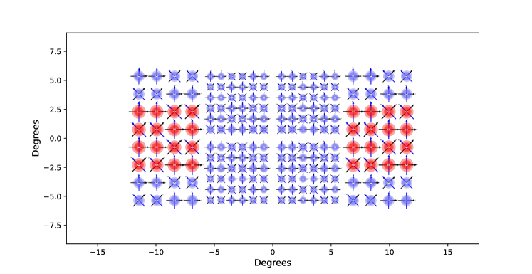
Figure 1: Focal plane layout of LFT. The circle represents the position of each pixel, which is sensitive to three bands (represented by circles proportional to beam size) in two linear polarization directions (by two arrows orthogonal to each other). The part used for the simulation in this study is the three pixels in the red area.

3 RESULTS

3.1 Input data

We simulated TODs consisting only of the CR noise for a 90-minute length for 12 detector channels on 3 pixels in a wafer (LF-1) of LFT (Fig. 1). Each channel represents one TES reading. In the simulation, one pixel stores four TES as shown in Fig. 3. Each TES reads antenna power of one of the two polarization orientations in one of the two frequencies (78 and 100 GHz) in one of the three pixels in the wafer as shown in Fig. 3. The LF-1 wafer actually stores 6$\times$6 pixels of three frequencies of two polarization pairs with a total of 216 TES channels without dark channels. For computational limitations, we simulated only 12 of them.

The LF-1 wafer has a size of 100$\times$100 mm² area and a depth of 2.5 mm made with Si. The wafer is thermally anchored to the heat bath at the four sides. We simulated the CR hits upon the LF-1 wafer following the GCR spectrum and flux obtained with the PAMELA experiment[10, 11]. We expect $\sim$400 s^-1 hit per wafer. Each CR event deposits energy, which spreads over the entire wafer as heat propagation. The average deposit energy is $\sim$1.3 MeV (0.2 pJ). The propagation is calculated using a finite element method, and the temperature beneath the 12 TES detector channels was derived as a function of time. Coupled differential equations —one describing the thermal coupling between the TES and the Si wafer beneath the TES and the other describing the electric circuit of TES under a constant bias current— were solved. As a result, we obtained TOD made only with CR events in the unit of power. The details of the simulation is given in Stever et al.[5].

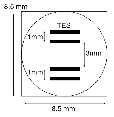
Figure 2: Position of TES in a pixel in the simulation. The circle represents the size of the lenslet for the pixel. The four parallel rectangles represent the TES. The pairs of top and bottom two are for the 78 and 100 GHz, respectively. Each pair reads two orthogonal directions of the linear polarization.

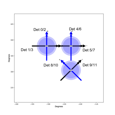
Figure 3: Part of the LF-1 wafer used in the simulation. Three pixels cover different positions of the sky separated by $\sim$0.75 arcdeg. Two polarization angles are shown with arrows, while two frequency bands are by circles proportional to the beam size. The assignment of the 12 channels is shown with the DetIDs.

The TOD in the time domain and its power spectrum are shown in Fig. 4. The TOD is simulated at a time resolution of 153 Hz, which is decimated from the original 20 MHz by a factor of 2¹⁷ by multiple stages of the cascaded integrator and comb filter. This is further decimated by a factor of 2³ to 19.1 Hz to match with our 20 Hz telemetry bandpass using a finite impulse response digital filter. In the current spacecraft design, the decimation by 2¹⁷ is performed by the warm electronics using FPGA, and the additional decimation by 2³ is by the payload module digital processing unit using CPU.

In the time domain, it is clearly seen that all 12 channels are strongly correlated. This is what we expect for LiteBIRD. The LF-1 wafer has 216 TES channels, all of which share a common Si wafer. At the temperature ($\sim$100 mK) of the Si wafer, the heat generated by a CR propagates fast. The traveling speed is much faster than the characteristic time scale of TES (a few ms) and the time resolution of the TOD (153 Hz) regardless of whether the propagation is by diffusion or ballistic process. Therefore, a single CR hit on the Si wafer affects all channels, which is almost synchronous in this time resolution. In the frequency domain, all channels show a flat spectrum with a power of $\sim$8.5 aW/$\sqrt{\mathrm{Hz}}$.

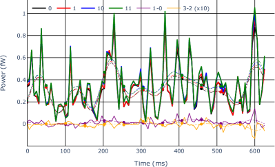
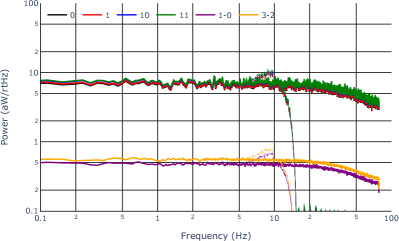
Figure 4: Input CR data in the time (left) and frequency (right) domains. The duration of time in the right is the same with two cycles of $4f_{\mathrm{HWP}}$ of LFT. Different channels are shown in different colors. Only four channels (det 0, 1, 10, 11) are shown for clarity. The difference between (0 and 1) and (2 and 3) is also shown. The 153 Hz data before decimation is shown by thick lines, while the 19 Hz date after decimation is by thin lines. The power can be converted to the equivalent thermo-dynamic temperature with a ratio of 0.2 aW $\sim$ 1 $\mu$K_CMB.

3.2 Output maps and power spectra

We simulated maps using TODs of a one-year length to have a coverage of the entire sky to calculate the angular power spectrum to the lowest scale of $l=2$. We produced one-year length TODs in two different methods. One (method A) is to shuffle and replicated the 90-minute TOD many times. This method is used when we evaluate the effects related to the common-mode nature of the CR noise in time. We first divided the TOD into ten pieces of a nine-minute length and selected one randomly 5840 times to make it a one-year length. There are $10^{5840}$ combinations of such selection and a sufficient number of realizations can be achieved in the simulation. All channels use the simulated data at the same time in order to preserve the correlation among them. This, however, produces artificial correlation in time within a given channel, despite the fact that the TODs are shuffled. When we need to remove this effect, we made the TODs with white noise randomly for the entire year for all the channels (method B). The amplitude of the white noise was set to 1.0 aW/$\sqrt{\mathrm{Hz}}$. In making $Q$ and $U$ maps, what matters is the differential mode of the TODs of two channels constituting a polarization pair (1–0 in Fig. 4 right), not the TOD of individual two channels (0 or 1). When there is no correlation between the two channels, the differential-mode TOD would have a white noise of an amplitude of $\sqrt{2}\times 8.5$ aW/$\sqrt{\mathrm{Hz}}$. When there is a strong correlation, as in the simulation, the differential-mode TOD has an amplitude of $\sim$0.5 aW/$\sqrt{\mathrm{Hz}}$. The simulation setup is not realistic enough to simulate the subtle difference between pair channels, so we tentatively use 1.0 aW/$\sqrt{\mathrm{Hz}}$ as an amplitude and interpret the result by scaling this value.

We used TOAST, which is a software framework for simulating and processing timestream data collected by telescopes. The sky is represented by pixels with an equal area based on the HEALPix [12] and its python implementation healpy library [13]. We used the pixelization parameter $N_{\mathrm{side}}=256$, which divides the entire sky with $N_{\mathrm{pix}}=12N_{\mathrm{side}}^{2}=786432$ pixels with an area corresponding to a square with a side of 13.7 arcmin. The angular scale up to $l_{\mathrm{max}}=767$ is obtained and the number of independent components in the spherical harmonic function is $N_{\mathrm{sph}}=(l_{\mathrm{max}}+2)(l_{\mathrm{max}}+1)/2=295296$.

LiteBIRD scans the sky by a combination of a spin, a precession, and a rotation around the Sun. The precession axis is along the anti-Sun direction, which moves at a speed of 360 deg year^-1. The precession rate is 192.348 min per rotation with an angle of 45 degrees. Along the precession axis, the satellite spins at a rate of 20 min per rotation with an angle of 50 degrees. The resultant sky coverage is depicted in the hit maps showing how many visits are made by detectors for each sky pixel in a given observation time (Fig. 5).

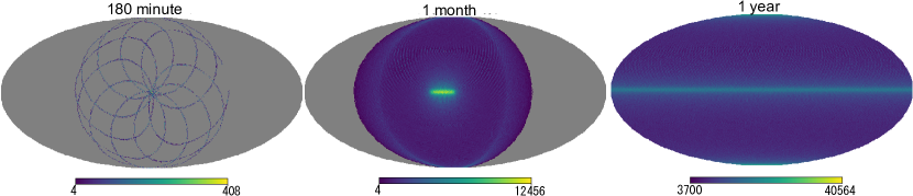
Figure 5: Hit maps over (left) 180 minutes, (middle) one month and (right) one year. The color bars indicate the number of visits for each pixel.

At a given time $t$, the satellite is observing at a sky position $p(t)$ characterized by the Stokes parameters $I(p)$, $Q(p)$, and $U(p)$. In LiteBIRD, the $U$ and $Q$ signals are further modulated by the HWP that is constantly rotating at a speed of $\omega_{\mathrm{HWP}}$. The $i$’th detector signal at a time $t$ is then given by

$$d_{i}(t)=I(p)+Q(p)\cos{2\psi_{i}}+U(p)\sin{2\psi_{i}}+n_{i}(t),$$ (1)

where $n_{i}(t)$ is the noise and $\psi_{i}(t)$ is the modulation angle given by

$$\psi_{i}(t)=\psi_{0}(t)+\psi_{i}+2\omega_{\mathrm{HWP}}t,$$ (2)

in which $\psi_{0}(t)$ is the relative angle of the focal plane to the sky, $\psi_{i}$ is the relative angle of the $i$’th detector to the focal plane. The modulation by HWP is $4f_{\mathrm{HWP}}=4\omega_{\mathrm{HWP}}/2\pi\sim$3.1 Hz for LFT. In the matrix form,

$$\bm{d}=\bm{P}(t,p)\bm{m}(p)+\bm{n},$$ (3)

where $\bm{m}(p)$ is a vector of the three Stokes parameters. The map making is a process to derive $\bm{m}(p)$ from observed $\bm{d}$. The simplest approach is to minimize

$$\chi^{2}=(\bm{d}-\bm{Pm})\bm{C}^{-1}_{\rm{n}}(\bm{d}-\bm{Pm}),$$ (4)

where $\bm{C}_{\rm{n}}=\langle\bm{n}\bm{n}^{T}\rangle$ is the noise covariance, and obtain the most plausible value of $\bm{m}(p)$ as

$$\tilde{\bm{m}}=(\bm{P}^{T}\bm{C}_{\rm{n}}^{-1}P)^{-1}P^{T}\bm{C}_{\rm{n}}^{-1}\bm{d}.$$ (5)

In making maps with TOAST from the simulated TOD (Fig. 4), we developed a new module so that we can feed noise as a time series. The map making was made separately for each day using multiprocessing and co-added in the map domain to make a one-year map. In this manner, we can complete the map making in a few hours using a personal computer equipped with 12 CPUs with a 3 GHz clock. We do not use the destriping technique developed mainly to mitigate long-term fluctuations such as 1/$f$ detector noise. More sophisticated algorithm can be developed in the future by making the full use of the features of the CR noise.

Fig.6 shows the resultant $T=I$, $Q$ and $U$ maps of one year made with the method B. The statistics of the maps are shown in Table 1. The monopole component is removed from the $T$ map, but not from the $Q$ and $U$ maps. Still, the mean value is small enough in the $Q$ and $U$ maps, indicating that they are made mostly from the differences of polarization pair channels that are balanced with each other. Finally, we calculated the power spectra using the anafast program of the healpy library. The program separates the $E$ and $B$ components and calculates the auto power spectra of $C_{l}^{TT}$, $C_{l}^{EE}$, and $C_{l}^{BB}$ as well as the cross power spectra of $C_{l}^{TE}$, $C_{l}^{TB}$, and $C_{l}^{EB}$. We show $C_{l}^{EE}$ and $C_{l}^{BB}$ relevant for the B-mode polarization detection.

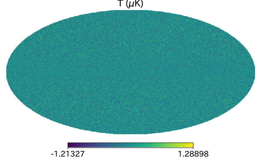
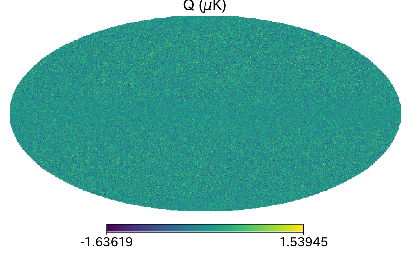
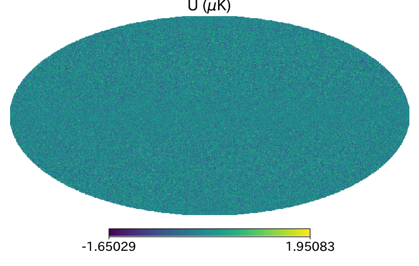
Figure 6: Simulated maps in the equatorial coordinate in the Mollweide projection: $T$ (left), $Q$ (middle), and $U$ (right) in the unit of $\mu$K_CMB.

Table 1: Statistics of the maps.

Map	Mean ($\mu$KCMB)	Min ($\mu$KCMB)	Max ($\mu$KCMB)	RMS ($\mu$KCMB)	$C_{l,est}$($\mu$K${}_{\mathrm{CMB}}^{2}$)
$T$	–1.4$\times 10^{-4}$	–1.2	1.2	0.23	2.4$\times 10^{-6}$
$Q$	–2.6$\times 10^{-4}$	–1.8	1.7	0.33	4.8$\times 10^{-6}$
$U$	–1.3$\times 10^{-4}$	–1.9	1.6	0.33	4.8$\times 10^{-6}$

4 DISCUSSION

4.1 Confirmation of results

4.1.1 Realizations

We first check how much fluctuation is expected in the simulation. We repeated the map-making with five different realizations of one-year TODs made the method B and compared the results in Fig 7. The power spectra values in both $C_{l}^{EE}$ and $C_{l}^{BB}$ fluctuates by a factor of a 2–3 at low-$l$, which provides an estimate of the uncertainty in the simulation.

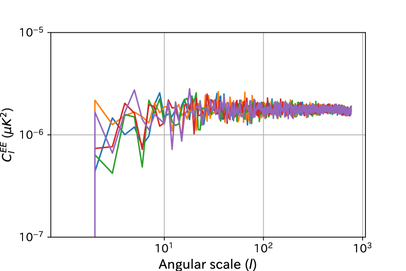
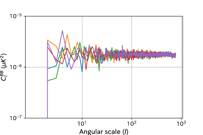
Figure 7: Power spectra of (left) $C_{l}^{EE}$ and (right) $C_{l}^{BB}$ for five different realizations of the one-year map simulation.

4.1.2 Values of output products

We next check if the values of the output products are consistent with the input TOD by an order estimate. First, the TOD has a power of $\sim$5.0 $\mu$K_CMB/$\sqrt{\mathrm{Hz}}$ at $4f_{\mathrm{HWP}}$ for the differential mode (1–0 or 3–2). This is relevant for estimating the noise in the $Q$ and $U$ maps because the two channels read two orthogonal directions at the same position at the same time in the same band (Fig. 3), hence their common mode is attributed more to the $I$ component and the differential mode to the $Q$ or $U$ component in Eqn. 1. In a one year observation, each sky pixel is exposed for $T_{\rm{pix}}=1\times 365\times 24\times 60\times 60/N_{\rm{pix}}\sim 40~{}\mathrm{s}$ on average. Therefore, the RMS value of the map is expected to be $\sim 5.0/\sqrt{2T_{\rm{pix}}N_{\mathrm{det}}}\sim 0.4~{}\rm{\mu K_{\mathrm{CMB}}}$ (Table. 1). Here, $N_{\mathrm{det}}=3$ is the number of detector pixels (see discussion below in § 4.2.2). This is consistent with the values in Table 1 for the $Q$ and $U$ maps. From the RMS of these maps, we can estimate the value of the coefficients of the spherical harmonic oscillator function as $|a_{lm,\mathrm{est}}|\sim\mathrm{RMS}\sqrt{4\pi/N_{\mathrm{sph}}}.$ From this, we can further estimate the value of angular power spectrum as $C_{l,\mathrm{est}}\sim|a_{lm,\mathrm{est}}|^{2}.$ The esitimated $C_{l,\mathrm{est}}$ is given in Table 1. The values for $Q$ and $U$ maps can be compared to $C_{l}^{EE}$ and $C_{l}^{BB}$ (Fig. 7) assuming that the fluctuation of $EE$ and $BB$ are equivalent to the that of $Q$ and $U$. They agree within a factor of a few.

4.1.3 Distribution of output products

We finally check that the $Q$ and $U$ maps by CR can be approximated as Gaussian, which was implicitly assumed when adopting the method B. We made maps using the TODs made with the method A, expecting that the distribution of the $a_{lm}$ follows the Gaussian. The distribution is shown in Fig. 8 separately for the real and imaginary parts and for $Q$ and $U$ maps, which is fitted very well with a single Gaussian function.

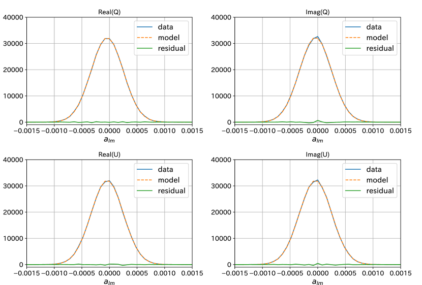
Figure 8: Distribution of $a_{lm}$ values of $Q$ (top) and $U$ (bottom) maps separately for the real (left) and imaginary (right) parts. The simulation results made with the method A are shown in blue, which is fitted with a single Gaussian model in orange. The residuals to the fit are in green.

4.2 Dependencies

4.2.1 On observation time

We first investigate the dependence of the angular power spectra on the observation time. As the TOD made with the method B is not correlated in the direction of time, we expect that the $C_{l}$ value will decrease proportionally to the inverse of the total integration time. We combined all the five one-year maps used in § 4.1 to simulate a five-year observation and compared the result with the one obtained with one year. The result is shown in Fig. 9. The $C_{l}$ value in the five-year observation was reduced from that in the one-year observation by a factor of $\sim$5 both in EE and BB as expected.

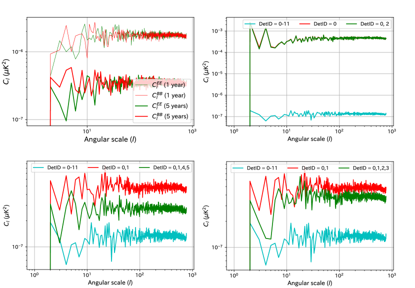
Figure 9: (Top left) Comparison of power spectra $C_{l}^{EE}$ (green) and $C_{l}^{BB}$ (red) for one-year (thin lines) and five-year (thick lines) observations using the method B. (Others) Comparison of power spectrum $C_{l}^{BB}$ for different subsets of detector channels using the method A.

4.2.2 On the number of detector channels

We next investigate the dependence on the number of detector channels. In this case, the situation is more complex, as all the detectors are strongly correlated (Fig. 4) in time. Some observe different polarization angle, sky position, or frequency band. To investigate the dependence, we used the TODs made with the method A and generated maps and power spectra from a subset of the 12 detector channels (Table 2). The detector identification (DetID) follows Fig. 3. The mean and the standard deviation of the TOD is slightly different among the 12 channels reflecting the fact that they are located in a different location in the LF-1 wafer; i.e., in the different distances from the thermal anchors on the four sides of the wafer. We normalized the TOD to remove the effects by this difference so that we can focus only on the dependence on the number of detectors.

Table 2: Mean and standard deviation over $l$ of $C_{l}^{BB}$ for subsets of detectors made with the method A.

Subset	Polarization	Pixel	Band	Mean ($\mu$K${}_{\mathrm{CMB}}^{2}$)	Standard deviation ($\mu$K${}_{\mathrm{CMB}}^{2}$)
0	1	1	1	5.1$\times 10^{-4}$	9.5$\times 10^{-5}$
0,2	1	1	2	4.7$\times 10^{-4}$	9.3$\times 10^{-5}$
0,1	2	1	1	4.8$\times 10^{-7}$	4.6$\times 10^{-8}$
0,1,2,3	2	1	2	3.8$\times 10^{-7}$	3.7$\times 10^{-8}$
0,1,4,5	2	2	2	2.7$\times 10^{-7}$	2.4$\times 10^{-8}$
0–11	2	3	2	1.3$\times 10^{-7}$	1.3$\times 10^{-8}$

First, we examine the angular power spectrum made only with DetID$=$0 (Fig. 9). The mean value of $C_{l}^{BB}$ is significantly elevated (Table 2). This is because a large part of the CR noise is attributed to $Q$ and $U$ in Eqn. 1. In contrast, when we use both orientations (DetID$=$0, 1), the value decreases as the dominant common-mode CR power is attributed preferentially to $I$.

Second, we compare the result with DetID$=$(0, 1) and DetID$=$(0, 1, 4, 5) in Fig. 9 and Table 2. In the latter set, the DetID$=$(0, 1) and (4, 5) pairs observe different positions of the sky at the same time. For a given position of the sky, the two pairs observe at different times, hence are not correlated. Therefore, the mean $C_{l}^{BB}$ value is reduced proportionally to the inverse of the pair number.

Third, we compare the result with DetID$=$(0, 1) and DetID$=$(0, 1, 2, 3) in Fig. 9 and Table 2. In the latter set, the DetID$=$(0, 1) and (2, 3) pairs observe the same position of the sky at the same time. The two pair differences 0–1 and 2–3 are not correlated as much as individual channels (Fig. 4a), thus some additional information can be obtained by adding another pair. Therefore, the mean $C_{l}^{BB}$ value is reduced to some extent.

Finally, we compare the results using all detector channels DetID $=$ 0–11 with the others. The mean $C_{l}^{BB}$ value is reduced by $\sim$3 times from DetID$=$(0, 1, 2, 3), suggesting that the power spectrum increases proportionally to the inverse of the number of sky positions observed at the same time.

4.3 Implications

In § 4.1, we confirmed that (i) the CR noise is nearly Gaussian in the $Q$ and $U$ map domain, and (ii) the values in the maps and the power spectra generated by TOAST are consistent with the input TOD. In § 4.2, we found that the power spectrum $C_{l}^{BB}$ by CR noise is reduced inverse-proportionally when we increase the integration time and the number of sky positions observed at the same time. If we assume that the input CR power is 1 aW/$\sqrt{\mathrm{Hz}}$ for the differential mode of two channels constituting a polarization pair, the expected $C_{l}^{\mathrm{BB}}\sim 2\times 10^{-6}~{}\mu$K${}_{\mathrm{CMB}}^{2}$ for one year observation with three pixels (Fig. 9a). This value scales with the exposure time and the number of pixels. If this is the case, the impact of the CR upon the B-mode measurement of an order of $\approx$10${}^{-6}\mu$K${}_{\mathrm{CMB}}^{2}$ would be at a manageable level, if not negligible.

1. The assumption of 1 aW/$\sqrt{\mathrm{Hz}}$ for the differential mode power of the paired polarization channels needs to be verified. This depends on the detailed design of the detectors, which is not included in the simulation yet.

2. The TOD of all detector channels are strongly coupled. This will bring a common-mode noise common among multiple frequency bands observed with the same detector pixel and pose a new challenge in separating CMB component from others in the spectrum.

3. Two sky positions at a fixed separation should be strongly correlated, as they are observed at the same time with a given pair of pixels. This is not evident in our result (Fig. 9) with only three pixels, but may emerge when more pixels are used.

4. The detector channels in a wafer have different responses due to the temperature gradient persistent over the wafer, which is anchored to the thermal bath only locally at the four sides. This will make the scaleability with the detector number more complex than a simple inverse law.

We expected there would be some extra correlations between sky pixels observed at the same by each of the pairs around $l\sim$200, but there are no features. If we use all of the pixels on the focal plane instead of just three, we may see some correlations.

5 SUMMARY

We presented an initial result of our end-to-end simulation of the CR noise. We presented details of the process from the TOD to maps and power spectra using TOAST. We examined the validity and scaleability of the products. We obtained several implications to make a more robust estimate, which need to be addressed in future studies.

Acknowledgments

We acknowledge useful comments by Aritoki Suzuki, Adrian Lee, Andrea Catalano, Reijo Keskitalo, Theodore Kisner, Giuseppe Puglisi, Hans Kristian Eriksen, and Masashi Hazumi.

Some of the results in this paper have been derived using the healpy and HEALPix package. This research used resources of (1) JAXA super computer system JSS2 for “Assessment of cosmic-ray for CMB observation satellite LiteBIRD” (code name: CWU10), (2) the National Energy Research Scientific Computing Center (NERSC), a U.S. Department of Energy Office of Science User Facility operated under Contract No. DE-AC02-05CH11231, (3) the Central Computing System owned and operated by the Computing Research Center at KEK.

This work is supported in Japan by ISAS/JAXA for Pre-Phase A2 studies, by the acceleration program of JAXA research and development directorate, by the World Premier International Research Center Initiative (WPI) of MEXT, by the JSPS Core-to-Core Program of A. Advanced Research Networks, and by JSPS KAKENHI Grant Numbers JP15H05891, JP17H01115, JP17H01125, and JP18K03715. The Italian LiteBIRD phase A contribution is supported by the Italian Space Agency (ASI Grants No. 2020-9-HH.0 and 2016-24-H.1-2018), the National Institute for Nuclear Physics (INFN) and the National Institute for Astrophysics (INAF). The French LiteBIRD phase A contribution is supported by the Centre National d’E tudes Spatiale (CNES), by the Centre National de la Recherche Scientifique (CNRS), and by the Commissariat à l’Energie Atomique (CEA). The Canadian contribution is supported by the Canadian Space Agency. The US contribution is supported by NASA grant no. 80NSSC18K0132. Norwegian participation in LiteBIRD is supported by the Research Council of Norway (Grant No. 263011). The Spanish LiteBIRD phase A contribution is supported by the Spanish Agencia Estatal de Investigación (AEI), project refs. PID2019-110610RB-C21 and AYA2017-84185-P. Funds that support the Swedish contributions come from the Swedish National Space Agency (SNSA/Rymdstyrelsen) and the Swedish Research Council (Reg. no. 2019-03959). The German participation in LiteBIRD is supported in part by the Excellence Cluster ORIGINS, which is funded by the Deutsche Forschungsgemeinschaft (DFG, German Research Foundation) under Germany’s Excellence Strategy (Grant No. EXC-2094-390783311).

References

- [1] Sugai, H., Ade, P. A. R., Akiba, Y., Alonso, D., Arnold, K., Aumont, J., Austermann, J., Baccigalupi, C., Banday, A. J., Banerji, R., Barreiro, R. B., Basak, S., Beall, J., Beckman, S., Bersanelli, M., Borrill, J., Boulanger, F., Brown, M. L., Bucher, M., Buzzelli, A., Calabrese, E., Casas, F. J., Challinor, A., Chan, V., Chinone, Y., Cliche, J.-F., Columbro, F., Cukierman, A., Curtis, D., Danto, P., de Bernardis, P., de Haan, T., De Petris, M., Dickinson, C., Dobbs, M., Dotani, T., Duband, L., Ducout, A., Duff, S., Duivenvoorden, A., Duval, J.-M., Ebisawa, K., Elleflot, T., Enokida, H., Eriksen, H. K., Errard, J., Essinger-Hileman, T., Finelli, F., Flauger, R., Franceschet, C., Fuskeland, U., Ganga, K., Gao, J.-R., Génova-Santos, R., Ghigna, T., Gomez, A., Gradziel, M. L., Grain, J., Grupp, F., Gruppuso, A., Gudmundsson, J. E., Halverson, N. W., Hargrave, P., Hasebe, T., Hasegawa, M., Hattori, M., Hazumi, M., Henrot-Versille, S., Herranz, D., Hill, C., Hilton, G., Hirota, Y., Hivon, E., Hlozek, R., Hoang, D.-T., Hubmayr, J., Ichiki, K., Iida, T., Imada, H., Ishimura, K., Ishino, H., Jaehnig, G. C., Jones, M., Kaga, T., Kashima, S., Kataoka, Y., Katayama, N., Kawasaki, T., Keskitalo, R., Kibayashi, A., Kikuchi, T., Kimura, K., Kisner, T., Kobayashi, Y., Kogiso, N., Kogut, A., Kohri, K., Komatsu, E., Komatsu, K., Konishi, K., Krachmalnicoff, N., Kuo, C. L., Kurinsky, N., Kushino, A., Kuwata-Gonokami, M., Lamagna, L., Lattanzi, M., Lee, A. T., Linder, E., Maffei, B., Maino, D., Maki, M., Mangilli, A., Martínez-González, E., Masi, S., Mathon, R., Matsumura, T., Mennella, A., Migliaccio, M., Minami, Y., Mistuda, K., Molinari, D., Montier, L., Morgante, G., Mot, B., Murata, Y., Murphy, J. A., Nagai, M., Nagata, R., Nakamura, S., Namikawa, T., Natoli, P., Nerval, S., Nishibori, T., Nishino, H., Nomura, Y., Noviello, F., O’Sullivan, C., Ochi, H., Ogawa, H., Ogawa, H., Ohsaki, H., Ohta, I., Okada, N., Okada, N., Pagano, L., Paiella, A., Paoletti, D., Patanchon, G., Piacentini, F., Pisano, G., Polenta, G., Poletti, D., Prouvé, T., Puglisi, G., Rambaud, D., Raum, C., Realini, S., Remazeilles, M., Roudil, G., Rubiño-Martín, J. A., Russell, M., Sakurai, H., Sakurai, Y., Sandri, M., Savini, G., Scott, D., Sekimoto, Y., Sherwin, B. D., Shinozaki, K., Shiraishi, M., Shirron, P., Signorelli, G., Smecher, G., Spizzi, P., Stever, S. L., Stompor, R., Sugiyama, S., Suzuki, A., Suzuki, J., Switzer, E., Takaku, R., Takakura, H., Takakura, S., Takeda, Y., Taylor, A., Taylor, E., Terao, Y., Thompson, K. L., Thorne, B., Tomasi, M., Tomida, H., Trappe, N., Tristram, M., Tsuji, M., Tsujimoto, M., Tucker, C., Ullom, J., Uozumi, S., Utsunomiya, S., Van Lanen, J., Vermeulen, G., Vielva, P., Villa, F., Vissers, M., Vittorio, N., Voisin, F., Walker, I., Watanabe, N., Wehus, I., Weller, J., Westbrook, B., Winter, B., Wollack, E., Yamamoto, R., Yamasaki, N. Y., Yanagisawa, M., Yoshida, T., Yumoto, J., Zannoni, M., and Zonca, A., “Updated Design of the CMB Polarization Experiment Satellite LiteBIRD,” Journal of Low Temperature Physics 199, 1107–1117 (may 2020).
- [2] Hazumi, M., Ade, P. A. R., Akiba, Y., Alonso, D., Arnold, K., Aumont, J., Baccigalupi, C., Barron, D., Basak, S., Beckman, S., Borrill, J., Boulanger, F., Bucher, M., Calabrese, E., Chinone, Y., Cho, S., Cukierman, A., Curtis, D. W., de Haan, T., Dobbs, M., Dominjon, A., Dotani, T., Duband, L., Ducout, A., Dunkley, J., Duval, J. M., Elleflot, T., Eriksen, H. K., Errard, J., Fischer, J., Fujino, T., Funaki, T., Fuskeland, U., Ganga, K., Goeckner-Wald, N., Grain, J., Halverson, N. W., Hamada, T., Hasebe, T., Hasegawa, M., Hattori, K., Hattori, M., Hayes, L., Hidehira, N., Hill, C. A., Hilton, G., Hubmayr, J., Ichiki, K., Iida, T., Imada, H., Inoue, M., Inoue, Y., Irwin, K. D., Ishino, H., Jeong, O., Kanai, H., Kaneko, D., Kashima, S., Katayama, N., Kawasaki, T., Kernasovskiy, S. A., Keskitalo, R., Kibayashi, A., Kida, Y., Kimura, K., Kisner, T., Kohri, K., Komatsu, E., Komatsu, K., Kuo, C. L., Kurinsky, N. A., Kusaka, A., Lazarian, A., Lee, A. T., Li, D., Linder, E., Maffei, B., Mangilli, A., Maki, M., Matsumura, T., Matsuura, S., Meilhan, D., Mima, S., Minami, Y., Mitsuda, K., Montier, L., Nagai, M., Nagasaki, T., Nagata, R., Nakajima, M., Nakamura, S., Namikawa, T., Naruse, M., Nishino, H., Nitta, T., Noguchi, T., Ogawa, H., Oguri, S., Okada, N., Okamoto, A., Okamura, T., Otani, C., Patanchon, G., Pisano, G., Rebeiz, G., Remazeilles, M., Richards, P. L., Sakai, S., Sakurai, Y., Sato, Y., Sato, N., Sawada, M., Segawa, Y., Sekimoto, Y., Seljak, U., Sherwin, B. D., Shimizu, T., Shinozaki, K., Stompor, R., Sugai, H., Sugita, H., Suzuki, A., Suzuki, J., Tajima, O., Takada, S., Takaku, R., Takakura, S., Takatori, S., Tanabe, D., Taylor, E., Thompson, K. L., Thorne, B., Tomaru, T., Tomida, T., Tomita, N., Tristram, M., Tucker, C., Turin, P., Tsujimoto, M., Uozumi, S., Utsunomiya, S., Uzawa, Y., Vansyngel, F., Wehus, I. K., Westbrook, B., Willer, M., Whitehorn, N., Yamada, Y., Yamamoto, R., Yamasaki, N., Yamashita, T., and Yoshida, M., “LiteBIRD: A Satellite for the Studies of B-Mode Polarization and Inflation from Cosmic Background Radiation Detection,” Journal of Low Temperature Physics 194, 443–452 (mar 2019).
- [3] Ade, P. A., Aghanim, N., Armitage-Caplan, C., Arnaud, M., Ashdown, M., Atrio-Barandela, F., Aumont, J., Baccigalupi, C., Banday, A. J., Barreiro, R. B., Battaner, E., Benabed, K., Benoît, A., Benoit-Lévy, A., Bernard, J. P., Bersanelli, M., Bielewicz, P., Bobin, J., Bock, J. J., Bond, J. R., Borrill, J., Bouchet, F. R., Bridges, M., Bucher, M., Burigana, C., Cardoso, J. F., Catalano, A., Challinor, A., Chamballu, A., Chiang, H. C., Chiang, L. Y., Christensen, P. R., Church, S., Clements, D. L., Colombi, S., Colombo, L. P., Couchot, F., Coulais, A., Crill, B. P., Curto, A., Cuttaia, F., Danese, L., Davies, R. D., De Bernardis, P., De Rosa, A., De Zotti, G., Delabrouille, J., Delouis, J. M., Désert, F. X., Diego, J. M., Dole, H., Donzelli, S., Doré, O., Douspis, M., Dupac, X., Efstathiou, G., Enßlin, T. A., Eriksen, H. K., Finelli, F., Forni, O., Frailis, M., Franceschi, E., Galeotta, S., Ganga, K., Giard, M., Girard, D., Giraud-Héraud, Y., González-Nuevo, J., Górski, K. M., Gratton, S., Gregorio, A., Gruppuso, A., Hansen, F. K., Hanson, D., Harrison, D., Henrot-Versillé, S., Hernández-Monteagudo, C., Herranz, D., Hildebrandt, S. R., Hivon, E., Hobson, M., Holmes, W. A., Hornstrup, A., Hovest, W., Huffenberger, K. M., Jaffe, A. H., Jaffe, T. R., Jones, W. C., Juvela, M., Keihänen, E., Keskitalo, R., Kisner, T. S., Kneissl, R., Knoche, J., Knox, L., Kunz, M., Kurki-Suonio, H., Lagache, G., Lamarre, J. M., Lasenby, A., Laureijs, R. J., Lawrence, C. R., Leonardi, R., Leroy, C., Lesgourgues, J., Liguori, M., Lilje, P. B., Linden-Vørnle, M., López-Caniego, M., Lubin, P. M., MacIás-Pérez, J. F., Mandolesi, N., Maris, M., Marshall, D. J., Martin, P. G., Martínez-González, E., Masi, S., Massardi, M., Matarrese, S., Matthai, F., Mazzotta, P., McGehee, P., Melchiorri, A., Mendes, L., Mennella, A., Migliaccio, M., Miniussi, A., Mitra, S., Miville-Deschênes, M. A., Moneti, A., Montier, L., Morgante, G., Mortlock, D., Mottet, S., Munshi, D., Murphy, J. A., Naselsky, P., Nati, F., Natoli, P., Netterfield, C. B., Nørgaard-Nielsen, H. U., Noviello, F., Novikov, D., Novikov, I., Osborne, S., Oxborrow, C. A., Paci, F., Pagano, L., Pajot, F., Paoletti, D., Pasian, F., Patanchon, G., Perdereau, O., Perotto, L., Perrotta, F., Piacentini, F., Piat, M., Pierpaoli, E., Pietrobon, D., Plaszczynski, S., Pointecouteau, E., Polenta, G., Ponthieu, N., Popa, L., Poutanen, T., Pratt, G. W., Prézeau, G., Prunet, S., Puget, J. L., Rachen, J. P., Racine, B., Reinecke, M., Remazeilles, M., Renault, C., Ricciardi, S., Riller, T., Ristorcelli, I., Rocha, G., Rosset, C., Roudier, G., Rusholme, B., Sanselme, L., Santos, D., Sauvé, A., Savini, G., Scott, D., Shellard, E. P., Spencer, L. D., Starck, J. L., Stolyarov, V., Stompor, R., Sudiwala, R., Sureau, F., Sutton, D., Suur-Uski, A. S., Sygnet, J. F., Tauber, J. A., Tavagnacco, D., Terenzi, L., Toffolatti, L., Tomasi, M., Tristram, M., Tucci, M., Umana, G., Valenziano, L., Valiviita, J., Van Tent, B., Vielva, P., Villa, F., Vittorio, N., Wade, L. A., Wandelt, B. D., Yvon, D., Zacchei, A., and Zonca, A., “Planck 2013 results. X. HFI energetic particle effects: Characterization, removal, and simulation,” Astronomy and Astrophysics 571, 31 (nov 2014).
- [4] Catalano, A., Ade, P., Atik, Y., Benoit, A., Bréele, E., Bock, J. J., Camus, P., Charra, M., Crill, B. P., Coron, N., Coulais, A., Désert, F. X., Fauvet, L., Giraud-Héraud, Y., Guillaudin, O., Holmes, W., Jones, W. C., Lamarre, J. M., Macías-Pérez, J., Martinez, M., Miniussi, A., Monfardini, A., Pajot, F., Patanchon, G., Pelissier, A., Piat, M., Puget, J. L., Renault, C., Rosset, C., Santos, D., Sauvé, A., Spencer, L., and Sudiwala, R., “Characterization and physical explanation of energetic particles on Planck HFI instrument,” Journal of Low Temperature Physics 176, 773–786 (sep 2014).
- [5] Stever, S. L., Ghigna, T., Tominaga, M., and Tsujimoto, M., “Simulations of systematic effects arising from cosmic rays in the LiteBIRD space telescope , and effects on the measurements of CMB B modes .,” JCAP (2021).
- [6] Lamarre, J. M., Puget, J. L., Ade, P. A., Bouchet, F., Guyot, G., Lange, A. E., Pajot, F., Arondel, A., Benabed, K., Beney, J. L., Benoît, A., Bernard, J. P., Bhatia, R., Blanc, Y., Bock, J. J., Bréelle, E., Bradshaw, T. W., Camus, P., Catalano, A., Charra, J., Charra, M., Church, S. E., Couchot, F., Coulais, A., Crill, B. P., Crook, M. R., Dassas, K., De Bernardis, P., Delabrouille, J., De Marcillac, P., Delouis, J. M., Désert, F. X., Dumesnil, C., Dupac, X., Efstathiou, G., Eng, P., Evesque, C., Fourmond, J. J., Ganga, K., Giard, M., Gispert, R., Guglielmi, L., Haissinski, J., Henrot-Versillé, S., Hivon, E., Holmes, W. A., Jones, W. C., Koch, T. C., Lagardère, H., Lami, P., Landé, J., Leriche, B., Leroy, C., Longval, Y., MacÍas-Pérez, J. F., MacIaszek, T., Maffei, B., Mansoux, B., Marty, C., Masi, S., Mercier, C., Miville-Deschênes, M. A., Moneti, A., Montier, L., Murphy, J. A., Narbonne, J., Nexon, M., Paine, C. G., Pahn, J., Perdereau, O., Piacentini, F., Piat, M., Plaszczynski, S., Pointecouteau, E., Pons, R., Ponthieu, N., Prunet, S., Rambaud, D., Recouvreur, G., Renault, C., Ristorcelli, I., Rosset, C., Santos, D., Savini, G., Serra, G., Stassi, P., Sudiwala, R. V., Sygnet, J. F., Tauber, J. A., Torre, J. P., Tristram, M., Vibert, L., Woodcraft, A., Yurchenko, V., and Yvon, D., “Planck pre-launch status: The HFI instrument, from specification to actual performance,” Astronomy and Astrophysics 520, 9 (sep 2010).
- [7] Ade, P. A., Aghanim, N., Arnaud, M., Ashdown, M., Aumont, J., Baccigalupi, C., Baker, M., Balbi, A., Banday, A. J., Barreiro, R. B., Bartlett, J. G., Battaner, E., Benabed, K., Bennett, K., Benoît, A., Bernard, J. P., Bersanelli, M., Bhatia, R., Bock, J. J., Bonaldi, A., Bond, J. R., Borrill, J., Bouchet, F. R., Bradshaw, T., Bremer, M., Bucher, M., Burigana, C., Butler, R. C., Cabella, P., Cantalupo, C. M., Cappellini, B., Cardoso, J. F., Carr, R., Casale, M., Catalano, A., Cayón, L., Challinor, A., Chamballu, A., Charra, J., Chary, R. R., Chiang, L. Y., Chiang, C., Christensen, P. R., Clements, D. L., Colombi, S., Couchot, F., Coulais, A., Crill, B. P., Crone, G., Crook, M., Cuttaia, F., Danese, L., D’Arcangelo, O., Davies, R. D., Davis, R. J., De Bernardis, P., De Bruin, J., De Gasperis, G., De Rosa, A., De Zotti, G., Delabrouille, J., Delouis, J. M., Désert, F. X., Dick, J., Dickinson, C., Dolag, K., Dole, H., Donzelli, S., Doré, O., Dörl, U., Douspis, M., Dupac, X., Efstathiou, G., Enßlin, T. A., Eriksen, H. K., Finelli, F., Foley, S., Forni, O., Fosalba, P., Frailis, M., Franceschi, E., Freschi, M., Gaier, T. C., Galeotta, S., Gallegos, J., Gandolfo, B., Ganga, K., Giard, M., Giardino, G., Gienger, G., Giraud-Héraud, Y., González, J., González-Nuevo, J., Górski, K. M., Gratton, S., Gregorio, A., Gruppuso, A., Guyot, G., Haissinski, J., Hansen, F. K., Harrison, D., Helou, G., Henrot-Versillé, S., Hernández-Monteagudo, C., Herranz, D., Hildebrandt, S. R., Hivon, E., Hobson, M., Holmes, W. A., Hornstrup, A., Hovest, W., Hoyland, R. J., Huffenberger, K. M., Jaffe, A. H., Jagemann, T., Jones, W. C., Juillet, J. J., Juvela, M., Kangaslahti, P., Keihänen, E., Keskitalo, R., Kisner, T. S., Kneissl, R., Knox, L., Krassenburg, M., Kurki-Suonio, H., Lagache, G., Lähteenmäki, A., Lamarre, J. M., Lange, A. E., Lasenby, A., Laureijs, R. J., Lawrence, C. R., Leach, S., Leahy, J. P., Leonardi, R., Leroy, C., Lilje, P. B., Linden-Vørnle, M., López-Caniego, M., Lowe, S., Lubin, P. M., MacÍas-Pérez, J. F., MacIaszek, T., MacTavish, C. J., Maffei, B., Maino, D., Mandolesi, N., Mann, R., Maris, M., Martínez-González, E., Masi, S., Massardi, M., Matarrese, S., Matthai, F., Mazzotta, P., McDonald, A., McGehee, P., Meinhold, P. R., Melchiorri, A., Melin, J. B., Mendes, L., Mennella, A., Mevi, C., Miniscalco, R., Mitra, S., Miville-Deschênes, M. A., Moneti, A., Montier, L., Morgante, G., Morisset, N., Mortlock, D., Munshi, D., Murphy, A., Naselsky, P., Natoli, P., Netterfield, C. B., Nørgaard-Nielsen, H. U., Noviello, F., Novikov, D., Novikov, I., O’Dwyer, I. J., Ortiz, I., Osborne, S., Osuna, P., Oxborrow, C. A., Pajot, F., Paladini, R., Partridge, B., Pasian, F., Passvogel, T., Patanchon, G., Pearson, D., Pearson, T. J., Perdereau, O., Perotto, L., Perrotta, F., Piacentini, F., Piat, M., Pierpaoli, E., Plaszczynski, S., Platania, P., Pointecouteau, E., Polenta, G., Ponthieu, N., Popa, L., Poutanen, T., Prézeau, G., Prunet, S., Puget, J. L., Rachen, J. P., Reach, W. T., Rebolo, R., Reinecke, M., Reix, J. M., Renault, C., Ricciardi, S., Riller, T., Ristorcelli, I., Rocha, G., Rosset, C., Rowan-Robinson, M., Rubiño-Martín, J. A., Rusholme, B., Salerno, E., Sandri, M., Santos, D., Savini, G., Schaefer, B. M., Scott, D., Seiffert, M. D., Shellard, P., Simonetto, A., Smoot, G. F., Sozzi, C., Starck, J. L., Sternberg, J., Stivoli, F., Stolyarov, V., Stompor, R., Stringhetti, L., Sudiwala, R., Sunyaev, R., Sygnet, J. F., Tapiador, D., Tauber, J. A., Tavagnacco, D., Taylor, D., Terenzi, L., Texier, D., Toffolatti, L., Tomasi, M., Torre, J. P., Tristram, M., Tuovinen, J., Türler, M., Tuttlebee, M., Umana, G., Valenziano, L., Valiviita, J., Varis, J., Vibert, L., Vielva, P., Villa, F., Vittorio, N., Wade, L. A., Wandelt, B. D., Watson, C., White, S. D., White, M., Wilkinson, A., Yvon, D., Zacchei, A., and Zonca, A., “Planck early results. I. The Planck mission,” Astronomy and Astrophysics 536, A1 (dec 2011).
- [8] Holmes, W. A., Bock, J. J., Crill, B. P., Koch, T. C., Jones, W. C., Lange, A. E., and Paine, C. G., “Initial test results on bolometers for the Planck high frequency instrument,” Applied Optics 47, 5996 (nov 2008).
- [9] Aghanim, N., Akrami, Y., Ashdown, M., Aumont, J., Baccigalupi, C., Ballardini, M., Banday, A. J., Barreiro, R. B., Bartolo, N., Basak, S., Benabed, K., Bernard, J. P., Bersanelli, M., Bielewicz, P., Bond, J. R., Borrill, J., Bouchet, F. R., Boulanger, F., Bucher, M., Burigana, C., Calabrese, E., Cardoso, J. F., Carron, J., Challinor, A., Chiang, H. C., Colombo, L. P., Combet, C., Couchot, F., Crill, B. P., Cuttaia, F., De Bernardis, P., De Rosa, A., De Zotti, G., Delabrouille, J., Delouis, J. M., Di Valentino, E., Diego, J. M., Doré, O., Douspis, M., Ducout, A., Dupac, X., Efstathiou, G., Elsner, F., Enßlin, T. A., Eriksen, H. K., Falgarone, E., Fantaye, Y., Finelli, F., Frailis, M., Fraisse, A. A., Franceschi, E., Frolov, A., Galeotta, S., Galli, S., Ganga, K., Génova-Santos, R. T., Gerbino, M., Ghosh, T., González-Nuevo, J., Górski, K. M., Gratton, S., Gruppuso, A., Gudmundsson, J. E., Handley, W., Hansen, F. K., Henrot-Versillé, S., Herranz, D., Hivon, E., Huang, Z., Jaffe, A. H., Jones, W. C., Karakci, A., Keihänen, E., Keskitalo, R., Kiiveri, K., Kim, J., Kisner, T. S., Krachmalnicoff, N., Kunz, M., Kurki-Suonio, H., Lagache, G., Lamarre, J. M., Lasenby, A., Lattanzi, M., Lawrence, C. R., Levrier, F., Liguori, M., Lilje, P. B., Lindholm, V., López-Caniego, M., Ma, Y. Z., Maciás-Pérez, J. F., Maggio, G., Maino, D., Mandolesi, N., Mangilli, A., Martin, P. G., Martínez-González, E., Matarrese, S., Mauri, N., McEwen, J. D., Melchiorri, A., Mennella, A., Migliaccio, M., Miville-Deschênes, M. A., Molinari, D., Moneti, A., Montier, L., Morgante, G., Moss, A., Mottet, S., Natoli, P., Pagano, L., Paoletti, D., Partridge, B., Patanchon, G., Patrizii, L., Perdereau, O., Perrotta, F., Pettorino, V., Piacentini, F., Puget, J. L., Rachen, J. P., Reinecke, M., Remazeilles, M., Renzi, A., Rocha, G., Roudier, G., Salvati, L., Sandri, M., Savelainen, M., Scott, D., Sirignano, C., Sirri, G., Spencer, L. D., Sunyaev, R., Suur-Uski, A. S., Tauber, J. A., Tavagnacco, D., Tenti, M., Toffolatti, L., Tomasi, M., Tristram, M., Trombetti, T., Valiviita, J., Vansyngel, F., Van Tent, B., Vibert, L., Vielva, P., Villa, F., Vittorio, N., Wandelt, B. D., Wehus, I. K., and Zonca, A., “Planck 2018 results: III. High frequency instrument data processing and frequency maps,” Astronomy and Astrophysics 641, A3 (sep 2020).
- [10] Casolino, M., De Simone, N., Bongue, D., Pia De Pascale, M., Di Felice, V., Marcelli, L., Minori, M., Picozza, P., Sparvoli, R., Castellini, G., Adriani, O., Bonechi, L., Bongi, M., Bottai, S., Papini, P., Ricciarini, S., Spillantini, P., Taddei, E., Vannuccini, E., Barbarino, G., Campana, D., Carbone, R., De Rosa, G., Osteria, G., Boezio, M., Bonvicini, V., Mocchiutti, E., Vacchi, A., Zampa, G., Zampa, N., Bruno, A., Saverio Cafagna, F., Ricci, M., Hofverberg, P., Pearce, M., Carlson, P., Bogomolov, E., Yu. Krutkov, S., N. Nikonov, N., I. Vasilyev, G., Menn, W., Simon, M., M. Galper, A., Grishantseva, L., Koldashov, S., Leonov, A., V. Mikhailov, V., A. Voronov, S., T. Yurkin, Y., G. Zverev, V., A. Bazilevskaya, G., N. Kvashnin, A., Maksumov, O., and Stozhkov, Y., “Two Years of Flight of the Pamela Experiment: Results and Perspectives,” Journal of the Physical Society of Japan 78, 35–40 (jan 2009).
- [11] Picozza, P., Galper, A. M., Castellini, G., Adriani, O., Altamura, F., Ambriola, M., Barbarino, G. C., Basili, A., Bazilevskaja, G. A., Bencardino, R., Boezio, M., Bogomolov, E. A., Bonechi, L., Bongi, M., Bongiorno, L., Bonvicini, V., Cafagna, F., Campana, D., Carlson, P., Casolino, M., De Marzo, C., De Pascale, M. P., De Rosa, G., Fedele, D., Hofverberg, P., Koldashov, S. V., Krutkov, S. Y., Kvashnin, A. N., Lund, J., Lundquist, J., Maksumov, O., Malvezzi, V., Marcelli, L., Menn, W., Mikhailov, V. V., Minori, M., Misin, S., Mocchiutti, E., Morselli, A., Nikonov, N. N., Orsi, S., Osteria, G., Papini, P., Pearce, M., Ricci, M., Ricciarini, S. B., Runtso, M. F., Russo, S., Simon, M., Sparvoli, R., Spillantini, P., Stozhkov, Y. I., Taddei, E., Vacchi, A., Vannuccini, E., Voronov, S. A., Yurkin, Y. T., Zampa, G., Zampa, N., and Zverev, V. G., “PAMELA - A Payload for Antimatter Matter Exploration and Light-nuclei Astrophysics,” Astroparticle Physics 27, 296–315 (aug 2006).
- [12] Gorski, K. M., Hivon, E., Banday, A. J., Wandelt, B. D., Hansen, F. K., Reinecke, M., and Bartelmann, M., “HEALPix: A Framework for High‐Resolution Discretization and Fast Analysis of Data Distributed on the Sphere,” The Astrophysical Journal 622, 759–771 (apr 2005).
- [13] Zonca, A., Singer, L., Lenz, D., Reinecke, M., Rosset, C., Hivon, E., and Gorski, K., “healpy: equal area pixelization and spherical harmonics transforms for data on the sphere in Python,” Journal of Open Source Software 4, 1298 (mar 2019).