Topological Defects Formation with Momentum Dissipation

Abstract

We employ holographic techniques to explore the effects of momentum dissipation on the formation of topological defects during the critical dynamics of a strongly coupled superconductor after a linear quench of temperature. The gravity dual is the dRGT massive gravity in which the conservation of momentum in the boundary field theory is broken by the presence of a bulk graviton mass. From the scaling relations of defects number and “freeze-out” time to the quench rate for various graviton masses, we demonstrate that the momentum dissipation induced by graviton mass has little effect on the scaling laws compared to the Kibble-Zurek mechanism. Inspired from Pippard’s formula in condensed matter, we propose an analytic relation between the coherence length and the graviton mass, which agrees well with the numerical results from the quasi-normal modes analysis. As a result, the coherence length decreases with respect to the graviton mass, which indicates that the momentum dissipation will augment the number of topological defects.

1 Introduction

Non-equilibrium dynamics of strongly coupled system is one of the most challenging tasks in theoretical physics. It is not only interesting in cosmology and particle physics, but also interesting within condensed matter physics henkel ; hohenberg ; Polkovnikov:2010yn . In recent years, the central question in understanding the strongly coupled theory was how the critical dynamics across a phase transition react to a time dependent coupling, i.e., a thermal or quantum quench. We investigate the critical dynamics of a strongly coupled superconducting phase transition within the AdS/CFT correspondence from string theory Maldacena:1997re , focusing on the formation and evolution of topological defects after a thermal quench. Spontaneous topological defect formation in such transition is a fundamental component of the celebrated Kibble-Zurek mechanism (KZM) Kibble:1976sj ; Kibble:1980mv ; Zurek:1985qw .

The basic idea of KZM is that: As a continuous symmetry is spontaneously broken during a second order phase transition, the evolution of the system stops being adiabatic and enters the “freeze-out” region as a result of the critical slowing down nearby the critical point. Topological defects will form at the interfaces where different symmetry-breaking domains meet and satisfy the “geodesic rule” Bowick:1992rz . KZM predicts a universal power law between the topological defects number and the quench rate. Such mechanism was first introduced by Kibble Kibble:1976sj ; Kibble:1980mv into Cosmology that as a result of relativistic causality, topological defects such as cosmic strings, monopoles, and etc., can form in the subsequent evolution of the Universe. It was later introduced by Zurek into condensed matter physics that the vortex lines may occur in a superfluid when the system is quenched, which is accessible in the laboratory Zurek:1985qw . This scenario was supported by various numerical studies Laguna:1996pv ; Yates:1998kx ; Ibaceta:1998yy ; Antunes:1998rz ; Donaire:2004gp ; Das:2011cx ; Gillman:2017ycq , and experiments carried out in a variety of systems Chuang:1991zz ; Bowick:1992rz ; Digal:1998ak ; Baeuerle:1996zz ; Ruutu:1995qz ; Carmi:2000zz ; Monaco:2002zz ; Maniv:2003zz ; Golubchik:2010zz ; Ado1 ; Ado2 .

The theory of KZM was proposed in a spatially homogenous background in which the momentum is conserved. However, real materials, which are composed of electrons, atom lattices, impurities and so on, do not possess such kind of momentum conservations (or have conservation only modulo the reciprocal lattice vectors) due to the spatial inhomogeneities MT . It will be quite important to investigate the KZM in the strongly coupled systems with momentum dissipation in the framework of holography. From holography, there have been a number of models built to study momentum dissipation by implementing the effects of translational symmetry breaking. Several approaches among these are to include the lattice effects Hartnoll:2012rj , or study the charge transport in the background of a spatially modulated bulk Horowitz:2012ky ; Horowitz:2012gs ; Horowitz:2013jaa ; Donos:2012js , or in the presence of impurities directly Hartnoll:2008hs ; Anantua:2012nj . However, due to the involved technics in such models, another conceptually distinct approach to holographic momentum dissipation was suggested in Vegh:2013sk . This approach does not make use of any conventional mechanism of translational symmetry breaking, but instead provides an effective bulk description of a theory without momentum conservation from massive gravity. Applications of gauge/gravity duality on non-equilibrium dynamics can be found in Liu:2018crr ; Guo:2018mip ; Gao:2019baf ; Lan:2020kwn ; Wittmer:2020mnm ; Ewerz:2020wyp ; Erdmenger:2020flu ; Ecker:2021ukv . Previous holographic work on KZM were carried out in Sonner:2014tca ; Chesler:2014gya ; Zeng:2019yhi ; Li:2019oyz ; delCampo:2021rak ; Xia:2020cjl ; Li:2021dwp , without any momentum dissipation in the background.

Holographic massive gravity exhibits momentum dissipation Davison:2013jba by giving a mass to the graviton. This mass breaks the diffeomorphism invariance of the gravitation theory, via the holographic dictionary, it in turn violates the conservation of energy-momentum in the dual field theory. Many clues have shown that the effect of massive graviton in the bulk gravity can be considered as the effect from the lattice in the dual field theory on the boundary Blake:2013owa ; Hu:2015dnl . Recently, a nonlinear massive gravity theory has been proposed by de Rham et.al. (dRGT theory) deRham:2010ik ; deRham:2010kj , and later it is found to be ghost-free Hassan:2011hr ; Hassan:2011tf . Note that, the dRGT massive gravity is thought to be the only healthy theory in Poincaré invariant setups, and there have been numerous studies in dRGT massive gravity which we will not list all of them Blake:2013bqa ; Cai:2014znn ; Hu:2015xva ; Xu:2015rfa ; Hendi:2015hoa .

Our goal in this paper is to explore the effect of the momentum dissipation (equivalently the effect of graviton mass) on the critical dynamics across a second-order phase transition after a linear quench of temperature from the holographic $(3+1)$-dimensional dRGT massive gravity. Quantized superconductor vortices will turn out due to KZM after quench. We will see that the momentum dissipation has little effect on the KZM scaling laws of the vortex number and “freeze-out” time to the quench rate. However, it is interesting to see that the coherence length $\hat{\xi}$ of the order parameter at the “freeze-out” time decreases with respect to the graviton mass $m$ from the quasi-normal modes (QNMs) analysis. Physically, it implies that the momentum dissipation will reduce the coherence length. Inspired from Pippard’s formula for the coherence length and mean free path abp , we propose an analytic expression between the coherence length $\hat{\xi}$ and the graviton mass $m$. This analytic relation is in good agreement with the results from QNMs analysis. Moreover, we also investigate the relations between the number of vortices $n$ and the graviton mass $m$ from both numerical simulations and analytic approach, and find that they fit very well as $m$ is not too large. The resulting vortex number will increase as graviton mass grows, which in turn indicates that momentum dissipation will enlarge the number of ovrtices.

The outline of the paper is as follows. In Sec.2, we briefly review the KZM, and build up the holographic model in the (3+1)-dimensional dRGT massive gravity in in Sec.3; Sec.4 contains the main analytical and numerical results of our paper to study the generations of vortices and the relations between graviton mass; The conclusions are drawn in Sec.5; In the Appendix A we briefly introduce the dRGT massive gravity.

2 A brief review of Kibble-Zurek mechanism

KZM is a paradigmatic theory to describe spontaneous generation of topological defects in non-equilibrium critical dynamics Kibble:1976sj ; Kibble:1980mv ; Zurek:1985qw . In the vicinity of critical point of a second-order phase transition, critical opalescence and critical slowing-down implies that the coherence length $\xi$ and the relaxation time $\tau$ diverge as

$$\xi(\epsilon)=\xi_{0}|\epsilon|^{-\nu},\qquad\tau(\epsilon)=\tau_{0}|\epsilon|^{-\nu z},$$ (1)

in which $\xi_{0}$ and $\tau_{0}$ are constant coefficients depending on the microscopic physics, while $\nu$ and $z$ are the static and dynamic critical exponents in equilibrium states, and $\epsilon$ is the dimensionless distance to the critical temperature, $\epsilon\equiv 1-T/T_{c}$. KZM assumes a linear quench across the critical point as $\epsilon(t)=t/\tau_{Q}$, in which $\tau_{Q}$ is the quench rate (or quench time). The “freeze-out” time occurs at the instant $\hat{t}$ when the relaxation time of the system $\tau$ equals the time scale of the quench to the critical point, then the dynamics approximately freezes (from nearly adiabatic to approximately impulse behavior within the time interval [$-\hat{t}$, $\hat{t}$]). Therefore, the “freeze-out” time can be readily obtained as

$$\hat{t}=(\tau_{0}\tau_{Q}^{\nu z})^{\frac{1}{1+\nu z}}.$$ (2)

The key insight of the KZM is that the average size $\hat{\xi}$ of the domains in the broken symmetry phase is set by the the equilibrium coherence length $\xi$ evaluated at the freeze-out time $\hat{t}$, i.e., $\hat{\xi}=\xi(\hat{t})$. Thus, the size of the symmetry-breaking domain is given by,

$$\hat{\xi}=\xi_{0}\left(\frac{\tau_{Q}}{\tau_{0}}\right)^{{\nu}/{(1+\nu z)}}$$ (3)

Topological defects will occur at the interfaces between various symmetry-breaking domains if they satisfy the “geodesic rules” Bowick:1992rz . Therefore, the above estimate of the $\hat{\xi}$ can be recast as an estimate for the resulting number of topological defects,

$$n\approx\frac{Ap}{\hat{\xi}^{d}}=\frac{Ap}{\xi_{0}^{d}}\left(\frac{\tau_{0}}{\tau_{Q}}\right)^{\frac{d\nu}{1+\nu z}}.$$ (4)

where $A$ is the volume size of the system, $p$ is the average probability for the domains to form defects and $d$ is the spatial dimension of the system. This relation is verified to be universal in various dimensions and for different kinds of topological defects Laguna:1996pv ; Yates:1998kx ; Ibaceta:1998yy ; Antunes:1998rz ; Donaire:2004gp ; Das:2011cx ; Gillman:2017ycq ; Chuang:1991zz ; Bowick:1992rz ; Digal:1998ak ; Baeuerle:1996zz ; Ruutu:1995qz ; Carmi:2000zz ; Monaco:2002zz ; Maniv:2003zz ; Golubchik:2010zz . In particular, the generated topological defects are vortices for superfluids or superconductors in $d=2$ system. We will investigate the KZM for vortices in a strongly coupled superconductor system with background momentum dissipation by virtue of the AdS/CFT technique in the following.

3 Holographic setup

The gravity background we adopt is the dRGT massive gravity in $(3+1)$-dimensional bulk spacetime deRham:2010ik ; deRham:2010kj (Please consult Appendix A for a brief review of dRGT massive gravity). In order to study the dynamics in this background, we work under the Vaidya-AdS solution with flat space $k=0$ and zero charge $q=0$ (We have scaled the AdS radius $L\equiv 1$.).

$$ds^{2}=\frac{1}{z^{2}}\left[-f(z)dt^{2}-2dtdz+\left(dx^{2}+dy^{2}\right)\right],$$ (5)

where

$$f(z)=1-Mz^{3}+\frac{c_{1}m^{2}}{2}z+c_{2}m^{2}z^{2},$$ (6)

in which $M$ is the mass parameter of the black hole, $c_{i}~{}(i=1,2)$ are constants and $m$ stands for the graviton mass. Location of the AdS boundary is $z=0$ while the horizon is $z=z_{+}$. Hawking temperature of the black brane thus is

$$T=\frac{1}{4\pi}\left(\frac{3}{z_{+}}+{c_{1}m^{2}}+{c_{2}m^{2}}z_{+}\right).$$ (7)

We work in the probe limit and adopt the conventional Maxwell-complex scalar action for holographic superconductors hartnoll

$$S_{\rm matter}=\int d^{4}x\sqrt{-g}\left[-\frac{1}{4}F_{\mu\nu}F^{\mu\nu}-|D_{\mu}\Psi|^{2}-m_{\psi}^{2}|\Psi|^{2}\right]$$ (8)

in which $F_{\mu\nu}=\partial_{\mu}A_{\nu}-\partial_{\nu}A_{\mu}$ is the Maxwell field strength, $A_{\mu}$ is the $U(1)$ gauge field, $D_{\mu}=\nabla_{\mu}-iA_{\mu}$ is the covariant derivative and $m_{\psi}$ is the mass of the complex scalar field $\Psi$. Thus, the equations of motion can be obtained

$$0 = (\nabla_{\mu}-iA_{\mu})(\nabla^{\mu}-iA^{\mu})\Psi-m_{\Psi}^{2}\Psi,$$ (9)

$$\nabla_{\nu}F^{\nu\mu} = i(\Psi^{\ast}(\nabla^{\mu}-iA^{\mu})\Psi-\Psi(\nabla^{\mu}+iA^{\mu})\Psi^{\ast}).$$ (10)

It is convenient to work in axial gauge by setting $A_{z}=0$, and take the ansatz for other fields as $\Psi=\Psi(t,z,x,y),A_{t,x,y}=A_{t,x,y}(t,z,x,y)$.

3.1 Holographic renormalization and boundary conditions

In order to solve the above equations, we need to impose suitable boundary conditions at the horizon $(z=z_{+})$ and at the AdS boundary $(z=0)$. Near the boundary $z\to 0$, fields can be expanded as,

$$\Psi=\Psi_{0}z^{\Delta_{-}}+\Psi_{1}z^{\Delta_{+}}+\mathcal{O}(z^{\Delta_{+}+1}),~{}~{}~{}A_{\mu}=a_{\mu}+b_{\mu}z+\mathcal{O}(z^{2}),$$ (11)

with $\Delta_{\pm}={\left(3\pm\sqrt{9+4m_{\psi}^{2}}\right)}/{2}$ are the conformal dimensions of dual scalar operators on boundary. Following the AdS/CFT dictionary, the interpretation of $\Psi_{0}$ is that it sources the symmetry breaking operator $\hat{O}$, while $a_{t}$ and $a_{i}$ are the chemical potential and superfluid velocity in the boundary, respectively. The physical meaning of $\Psi_{1}$ and $b_{\mu}$ will be clear after the holographic renormalization.

From holographic renormalization Skenderis:2002wp , varying the renormalized on-shell action with respect to the source terms one can achieve the corresponding conjugate variables. In order to obtain finite on-shell action, we should add the counter terms of the scalar fields $S_{\rm ct}=\int d^{3}x\sqrt{-\gamma}\Psi^{*}\Psi$ into the divergent on-shell action, where $\gamma$ is determinant of the reduced metric on the boundary. We set Neumann boundary conditions for gauge fields in order to get the dynamical gauge fields in the boundary. In order to have a well-defined variation, the surface term $S_{\rm sf}=\int d^{3}x\sqrt{-\gamma}n^{\mu}F_{\mu\nu}A^{\nu}$ should also be added, where $n^{\mu}$ is the normal vector perpendicular to the boundary. Hence, we can get the finite renormalized on-shell action $S_{\rm ren}$. The expectation value of the order parameter can be obtained from the holographic renormalization by varying $S_{\rm ren}$ with respect to $\Psi_{0}$, resulting in $\langle\hat{O}\rangle=\Psi_{1}$.

We impose $\Psi_{0}=0$ all time in order to have a spontaneous symmetry breaking of the order parameter. This translates into a homogenous Dirichlet boundary condition for the field $\Psi$ in the AdS boundary, i.e., $\Psi|_{z=0}=0$. Expanding the $z$-component of the Maxwell equations near boundary, we reach $\partial_{t}b_{t}+\partial_{i}J^{i}=0$, which is exactly a conservation equation of the charge density $\rho$ and current $J^{i}$ on the boundary, since from the variation of $S_{\rm ren}$ one can get $b_{t}=-\rho$ and $J^{i}=-b_{i}-(\partial_{i}a_{t}-\partial_{t}a_{i})$. At the horizon, we demand the regularity of the fields. Since the metric component $g_{tt}$ is zero at the horizon, the component $A_{t}$ should be vanishing, while other fields are finite at the horizon.

3.2 Numerical schemes

We choose $m_{\psi}^{2}=-2$ without loss of generality and set $c_{1}=1,c_{2}=-1/2$ in order to make the background thermodynamically stable Hu:2015dnl ; Cai:2014znn . For convenience of the numerical calculation, we set the black hole mass parameter as $M=1$ and the location of horizon at $z_{+}=1$. From holographic superconductor hartnoll , increasing the chemical potential or the charge density equals decreasing the temperature of the system. We choose to increase the charge density $\rho$ in our paper. In addition, the temperature of the black hole $T$ has the mass dimension one while the charge density $\rho$ has mass dimension two from the dimensional analysis. Therefore, in order to linearize the temperature near the critical point according to KZM, we quench the charge density $\rho$ as $\rho(t)=\rho_{c}(1-t/\tau_{Q})^{-2}$, where $\rho_{c}$ is the critical charge density for the static and homogeneous holographic superconducting system. We should note that different graviton masses $m$ correspond to different $\rho_{c}$, which is shown in Fig.1

Figure 1: Critical charge density versus graviton mass. Red dots are numerical results while the blue line is a fitted critical curve. Upper the critical curve the system is in a superconducting phase while below the curve it is in a normal metal phase (shaded region).

We quench the system from normal state with initial temperature $T_{i}=1.4T_{c}$ to superconducting state with the final equilibrium temperature $T_{f}=0.8T_{c}$. The size of the boundary system is $(x,y)=(50,50)$. We take advantage of the Chebyshev pseudo-spectral method in the radial direction $z$ and use the Fourier decomposition in the $(x,y)$-directions since the periodic boundary condition is imposed along $(x,y)$-directions. The grids in $z$-direction is 21 while the grids along $(x,y)$-directions are $201\times 201$. We thermalize the system by adding random seeds for the fields at the initial time. The random seeds are sampled in the bulk by satisfying the white noise distributions $\langle s(t,\vec{x})\rangle=0$ and $\langle s(t,\vec{x})s(t^{\prime},\vec{x}^{\prime})\rangle=\zeta\delta(t-t^{\prime})\delta(\vec{x}-\vec{x}^{\prime})$, with the amplitude $\zeta\approx 10^{-3}$. The system evolves by using the 4th order Runge-Kutta method with time step $\Delta t=0.01$. Filtering of the high momentum modes are implemented following the “2/3’s rule” that the uppermost one third Fourier modes are removed Chesler:2013lia .

4 Results

4.1 KZM scalings of vortex number and “freeze-out” time

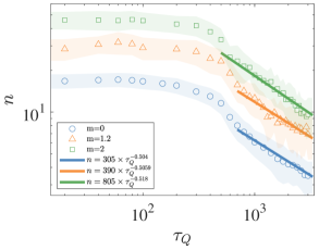
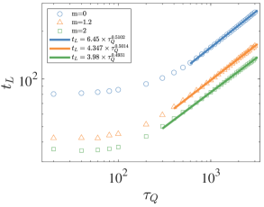
Figure 2: (Left panel) Double logarithmic relation between vortex number $n$ and quench time $\tau_{Q}$ for graviton mass $m=(0,1.2,2)$. The circles, triangles and squares are the numerical data while the straight lines are the best fitted lines in the slow quench regime (larger $\tau_{Q}$). The shaded regions represent the standard deviations away from the mean values. For the slow quench, the scaling relations satisfy the KZM scaling laws very well; However, for fast quench (smaller $\tau_{Q}$), vortex number $n$ is almost constant beyond the scope of KZM. (Right panel) Double logarithmic relation between the lag time $t_{L}$ and quench rate $\tau_{Q}$. For slow quench the relation between $t_{L}$ and $\tau_{Q}$ satisfy the KZM scalings very well, while for fast quench $t_{L}$ keeps almost constant. This figure was obtained by running $100$ times of simulations for each $\tau_{Q}$ and $m$.

In this subsection, we will examine the KZM scaling laws in Eqs.(2) and (4), depending on the graviton mass. We count the vortex number $n$ as the order parameter $\langle\hat{O}\rangle$ saturates to its equilibrium value. Scalings between the number $n$ and quench time $\tau_{Q}$ under different graviton mass $m$ are exhibited in the left panel of Fig.2. The shaded regions correspond to the standard deviations from the mean values. In the fast quench regime (small $\tau_{Q}$) the vortex number approximately saturates due to the finite size effect, which is consistent with previous results in condensed matter or holography Chesler:2014gya ; Sonner:2014tca ; Zeng:2019yhi ; Li:2019oyz . However, in the slow quench regime (large $\tau_{Q}$), the vortex number will decrease with respect to quench time satisfying the scaling relations as $n_{m=0}\approx 305\times\tau_{Q}^{-0.504}$, $n_{m=1.2}\approx 390\times\tau_{Q}^{-0.5059}$ and $n_{m=2}\approx 805\times\tau_{Q}^{-0.518}$ respectively. From this figure, we can conclude that as $m$ grows, or equivalently momentum dissipation gets stronger, the number of vortices will increase as well. In other words, from the relation $n\propto 1/\hat{\xi}^{2}$ we can deduce that the momentum dissipation will reduce the coherence length. We will study this relation between coherence length and the graviton mass in the next subsection in details.

The “freeze-out” time $\hat{t}$ can be reflected by studying the lag time $t_{L}$ that defined as order parameter begins to grow rapidly Das:2011cx ; Sonner:2014tca ; Zeng:2019yhi . In numerics we operationally set $t_{L}$ as $\langle\hat{O}\rangle\sim 0.1$ following Sonner:2014tca ; Zeng:2019yhi ; Das:2011cx . On the right panel of Fig.2 we exhibit the relation between $t_{L}$ and $\tau_{Q}$. The error bars are not shown since they are very tiny. We see that for fast quench the lag time is almost constant for different $m$’s. However, for slow quench, one can read that $t_{L}\approx 6.45\times\tau_{Q}^{0.5102}$ for $m=0$, $t_{L}\approx 4.347\times\tau_{Q}^{0.5014}$ for $m=1.2$ and $t_{L}\approx 3.98\times\tau_{Q}^{0.4931}$ for $m=2$. Therefore, from the two KZM scaling relations in Eqs.(2) and (4), one can readily evaluate the dynamic critical exponent $z$ and the static critical exponent $\nu$ on the boundary as $(\nu\approx 0.514496,z\approx 2.0246),(\nu\approx 0.50732,z\approx 1.98221)$ and $(\nu\approx 0.510949,z\approx 1.90386)$ for $m=(0,1.2,2)$ respectively, in which the exponent matches the mean-field theory values with $z=2$ and $\nu=1/2$. This means graviton mass in dRGT massive gravity does not alter the KZM scaling laws, which in turn indicates that the existence of graviton mass does not affect critical exponents, $z$ and $\nu$, in the boundary field theory. The boundary field theory remains as a mean-field theory, which is consistent with the assumption of AdS/CFT correspondence that the boundary is a mean-field theory in large $N$ limit Zaanen:2015oix .

4.2 Coherence length and graviton mass

4.2.1 Quasi-normal modes analysis

From previous section 2, we see that the average size of the symmetry-breaking domains $\hat{\xi}$ is approximately the coherence length of the order parameter at the “freeze-out” time $\hat{t}$ Zurek:1985qw . Fortunately, from holography one can compute the coherence length from QNMs of the scalar field in the bulk by choosing suitable boundary conditions Kovtun:2005ev ; Maeda:2009wv . The QNMs correspond to the poles of the retarded Green’s function of the dual field theory. One can read off the coherence length $\xi$ from the correlation function

$$\langle O(\omega,k)O^{\dagger}(-\omega,-k)\rangle\sim\frac{1}{i\tilde{c}\omega+k^{2}+1/\xi^{2}}.$$ (12)

where $k$ and $\omega$ are the momentum and frequency of perturbation modes respectively, while $\tilde{c}$ is a parameter. QNMs are computed from small fluctuations of the background fields, such that $\Psi(t,z,x)=\psi_{0}(z)+\psi(z)e^{-i\omega t+ikx}$, where $\psi_{0}(z)$ is the static background of scalar field while $\psi(z)e^{-i\omega t+ikx}$ is small fluctuations with respect to the background. For simplicity, we have assumed the fluctuations as plane waves in the only $x$-direction. We calculate the QNMs in the symmetric phase, i.e., in the normal phase that the background $\psi_{0}(z)$ is vanishing. This is because from KZM, dynamics ceases to be adiabatic and enters an impulse stage within the time interval [$-\hat{t}$, $\hat{t}$] as we learned from previous section 2. The starting of the symmetry breaking will occur at the instant $t\approx-\hat{t}$, which is in the normal phase before the critical point. This greatly simplifies the complexity of the calculations.

It is convenient to work out the QNMs in the Schwarzschild-AdS metric of the spacetime Sonner:2014tca ; Zeng:2019yhi . Substituting the scalar field $\Psi(t,z,x)$ into the EoMs (9),(10), and extracting the first order of the perturbations $\psi(z)$, we arrive at the decoupled linear equation as

$$\psi^{\prime\prime}+\frac{f^{\prime}}{f}\psi^{\prime}+\left(\frac{(A_{t}+\omega)^{2}}{f^{2}}+\frac{zf^{\prime}-k^{2}z^{2}+2}{z^{2}f}-\frac{2}{z^{2}}\right)\psi=0$$ (13)

in which $A_{t}$ is the background gauge field. We impose the ingoing boundary conditions at the horizon $z_{+}=1$,

$$\psi_{z_{+}}=(z-1)^{-\frac{iw}{4\pi T}}(1+\mathcal{O}(z-1)),$$ (14)

where $T$ is the Hawking temperature of black hole. Vanishing boundary conditions are imposed at the boundary $z=0$. We adopt the determinant method Zeng:2019yhi to calculate the QNMs and fix the quench rate as $\tau_{Q}=20$ (other quench rates will have similar results). More specifically, we employ the Chebyshev differential matrix to convert the differentiation with respect to spacetime coordinate into a matrix. Zeros of the determinant of the resulting matrix are the QNMs after imposing the above boundary conditions. The lowest mode in the QNMs makes the most contribution to the perturbations. In practice, the lowest mode is the mode that is closest to the real axis. We can evaluate the coherence length from Eq.(12) by setting $\omega=0$, and arrive at $\hat{\xi}=1/|{\rm Im}(k^{*})|$ where $k^{*}$ is the lowest mode in those QNMs. After solving the Eq.(13) one can get a series of QNMs in the complex $k$-plane, as is shown in the left panel of Fig.3 for $m=2$. The red dots, symmetric and closest to the real axis, stand for the lowest poles $k^{*}$. Other sub-leading poles (in blue squares), all locate in the imaginary axis, are also symmetric to the real axis. Different graviton masses correspond to different series of QNMs, leading to a relation between coherence lengths and $m$, i.e., $\hat{\xi}=\hat{\xi}(m)$, which are shown as red dots in the right panel of Fig.3.

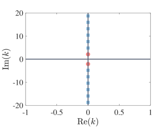
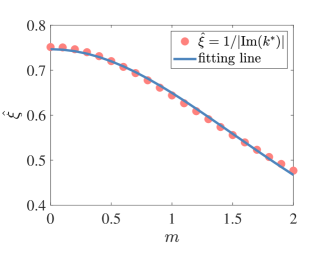
Figure 3: (Left panel) QNMs in the complex $k$-plane for $m=2$ and $\omega=0$. The leading poles nearest the real axis, marked by red dots, determine the behavior of correlations at large distances. The blue squares are the sub-leading poles which are not important to the correlations. (Right panel) Coherence length $\hat{\xi}$ of the order parameter at the “freeze-out” time versus the graviton mass $m$. The red dots represent $\hat{\xi}=1/|{\rm Im}(k^{*})|$, where $k^{*}$ are the leading QNMs, and the blue line is the fitting line $\hat{\xi}\approx 0.7466/(1+0.1496m^{2})$ from Eq.(17). For both panels, we fix the quench rate as $\tau_{Q}=20$.

4.2.2 Analytic relation between $\hat{\xi}$ and $m$

The analytic relation between the coherence length $\hat{\xi}$ and the graviton mass $m$ was seldom discussed. In Hu:2015dnl , the authors found that the coherence length would decrease with respect to the graviton mass in the system of a holographic Josephson junction. However, they did not propose an analytic relation between $\hat{\xi}$ and $m$. In this subsection, we will seek this analytic relation between $\hat{\xi}$ and $m$ and show that this relation matches well with the numerical results from QNMs analysis.

From the discussions in Vegh:2013sk ; Davison:2013jba ; Blake:2013owa , the graviton mass $m$ effectively plays a role of momentum dissipation in the boundary field theory. This momentum dissipation might be from scatterings of electrons to lattices or impurities, which lead to the assumption in Drude model that the relation between the mean free path $l$ and scattering time $\tau_{s}$ is $\tau_{s}=l/V_{F}$, in which $V_{F}$ is the Fermi velocity MT . In condensed matter physics, the coherence length $\xi$ can be related to the mean free path $l$ from Pippard’s formula abp ; MT ,

$$\frac{1}{\xi}=\frac{1}{\xi_{p}}+\frac{1}{\alpha l},$$ (15)

where $\xi_{p}$ is the coherence length of a pure material without any scatterings, and $\alpha$ is a numerical constant. Then from the relation $\tau_{s}=l/V_{F}$ in Drude model, we get

$$\xi=\frac{\xi_{p}}{1+\frac{\xi_{p}}{\alpha V_{F}}\,\tau_{s}^{-1}}$$ (16)

Fortunately, from holography Blake:2013bqa $\tau_{s}$ can be related to the graviton mass $m$ as $\tau_{s}^{-1}=\gamma m^{2}$ where $\gamma$ is a coefficient independent of $m$. Therefor, we finally reach

$$\xi=\frac{a}{1+bm^{2}}.$$ (17)

where $a=\xi_{p}$ and $b={\xi_{p}\gamma}/(\alpha V_{F})$. The fitting of this relation (17) is exhibited as blue line in the right panel of Fig.3, with fitting parameters as $a\approx 0.7466$ and $b\approx 0.1496$. From Fig.3 we see that the numerical results (red dots) from QNMs analysis are fitted very well with the analytic relation Eq.(17). Therefore, the coherence length $\hat{\xi}$ at the “freeze-out” time will decrease as $m$ increases. This also means stronger momentum dissipation in the boundary field will reduce the average size of the symmetry-breaking domains, which in turn implies that the vortex number $n$ would grow with respect to graviton mass according to $n\varpropto 1/\hat{\xi}^{2}$ in Eq.(4).

4.3 Vortex number and graviton mass

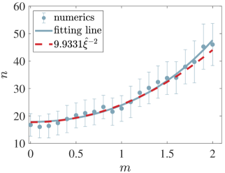
Figure 4: Vortex number $n$ versus the graviton mass $m$. Blue solid dots and error bars are from numerical data while blue line is the best fit as $n\approx 17.82\times\left(1+0.1585m^{2}\right)^{2}$. Error bars denote the standard deviations. From the relation $n\approx Ap\hat{\xi}^{-2}$ in Eq.(4), the numerical data from QNMs analysis in the right panel of Fig.3 can be recast into the red dashed line to link the relations between $n$ and $m$. The blue solid line matches very well with the red dashed line as $m\lesssim 1.5$. The quench rate in this figure is the same as in Fig.3, i.e., $\tau_{Q}=20$.

We count the vortex number at the final equilibrium state of the system, where the order parameter is well developed. From the above analysis, we expect that the vortex number $n$ would increase with the graviton mass, and satisfying the following relation via Eq.(4) and Eq.(17):

$$n\approx\frac{Ap}{\hat{\xi}^{2}}=\frac{Ap}{a^{2}}\left(1+bm^{2}\right)^{2}$$ (18)

The numerical results of the vortex number $n$ versus the graviton mass $m$ are shown as solid blue dots in Fig.4 with error bars presenting the standard deviations. The solid blue line is the fitting relation of the numerical results as $n=17.82\times\left(1+0.1585m^{2}\right)^{2}$ from Eq.(18). Compared to the above $b\approx 0.1496$ in Eq.(17) from the right panel of Fig.3, we can see that the values of the coefficient before $m^{2}$ are close to each other within $5.6151\%$ errors. Estimates of parameter $b$ from these two methods, i.e., one is from the fitting of relation $n\sim m$, the other is from the fitting of $\hat{\xi}\sim m$, match each other very well! This also indicates that our conjecture of the relation between coherence length and graviton mass, viz. Eq.(17) is very trustable.

The overall factor in the front of Eq.(18) can even provide us the estimate of the probability $p$, which is the probability for the symmetry-breaking domains to form vortices, in Eq.(4). We already knew $a\approx 0.7466$ in Eq.(17) from the right panel of Fig.3, and the size of the system is $A=50\times 50=2500$, thus we can readily get $p\approx 17.82\times 0.7466^{2}/2500\approx 0.003973$ and $n\approx Ap/\hat{\xi}^{2}\approx 9.9331\hat{\xi}^{-2}$. The later relation is plotted as red dashed line in the Fig.4, where $\hat{\xi}$ comes from the QNMs analysis in the right panel of Fig.3. We see that the red dashed line fits very well with the blue fitting line except in the large regime of $m$, such as $m>1.5$. This discrepancy originates from the differences between the two fitted values of $b$, i.e, $b\approx 0.1496$ from Eq.(17) and $b\approx 0.1585$ from Eq.(18). However, the error between these two $b$’s is small, therefore, it is fair to say that our assumption of the relation between the coherence length and the graviton mass, viz. Eq.(17) is reliable.

5 Conclusions and discussions

In summary, we have investigated the effects of momentum dissipation induced by the graviton mass on the critical dynamics in the background of a $(3+1)$-dimensional dRGT massive gravity by taking advantage of the AdS/CFT correspondence. The KZM scaling laws of the vortex number and the “freeze-out” time with respect to the quench rate were not affected by the graviton mass. This in turn indicated that the static and dynamic critical exponents were not changed by the existence of graviton mass. It further implied that the boundary field theory was always like a mean-field theory in spite of the graviton mass.

However, the outcome of vortex numbers depended on the graviton mass, since momentum dissipation would shrink the size of the symmetry-breaking domains. Inspired from Pippard’s formula on the coherence length and the mean free path, we proposed an analytical relation between the coherence length and the graviton mass. This relation was verified from the QNMs analysis of the perturbations of the scalar field, which was a key result in our paper. We further investigated the relation between the number of vortices and the graviton mass both analytically and numerically, and the results were consistent with each other. Therefore, in conclusion, the momentum dissipation induced by graviton mass would increase the number of vortices, although it would not affect the KZM scaling laws.

Appendix A A Brief Review of dRGT massive Gravity

Let us consider the action for an $(n+2)$-dimensional ghost-free dRGT massive gravityVegh:2013sk ; Cai:2014znn

$$S=\frac{1}{16\pi G}\int d^{n+2}x\sqrt{-g}\left[R+\frac{n(n+1)}{L^{2}}-\frac{1}{4}F^{2}+m^{2}\sum_{i}^{4}c_{i}\mathcal{U}_{i}(g,\textbf{f})\right],$$ (19)

where $L$ is the radius of the AdS_n+2 spacetime, $m$ stands for the graviton mass parameter, f is a fixed symmetric tensor usually called the reference metric, $c_{i}$ are constants, and $\mathcal{U}_{i}$ are symmetric polynomials of the eigenvalues of the $(n+2)\times(n+2)$ matric $\mathcal{K}^{\mu}_{~{}\nu}\equiv\sqrt{g^{\mu\alpha}\textbf{f}_{\alpha\nu}}$:

$$\mathcal{U}_{1} = [\mathcal{K}],$$

$$\mathcal{U}_{2} = [\mathcal{K}]^{2}-[\mathcal{K}^{2}],$$

$$\mathcal{U}_{3} = [\mathcal{K}]^{3}-3[\mathcal{K}][\mathcal{K}^{2}]+2[\mathcal{K}^{3}],$$

$$\mathcal{U}_{4} = [\mathcal{K}]^{4}-6[\mathcal{K}^{2}][\mathcal{K}]^{2}+8[\mathcal{K}^{3}][\mathcal{K}]+3[\mathcal{K}^{2}]^{2}-6[\mathcal{K}^{4}].$$ (20)

The square root in $\mathcal{K}$ means $(\sqrt{A})^{\mu}_{~{}\nu}(\sqrt{A})^{\nu}_{~{}\lambda}=A^{\mu}_{~{}\lambda}$ and $[\mathcal{K}]=K^{\mu}_{~{}\mu}=\sqrt{g^{\mu\alpha}\textbf{f}_{\alpha\mu}}$. The equations of motion turn out to be

$$R_{\mu\nu}-\frac{1}{2}Rg_{\mu\nu}-\frac{n(n+1)}{2L^{2}}g_{\mu\nu}-\frac{1}{2}\left(F_{\mu\sigma}F_{\nu}^{\ \sigma}-\frac{1}{4}g_{\mu\nu}F^{2}\right)+m^{2}\chi_{\mu\nu} = 8\pi GT_{\mu\nu},$$ (21)

$$\nabla_{\mu}F^{\mu\nu} = 0,$$ (22)

where

$$\chi_{\mu\nu} = -\frac{c_{1}}{2}(\mathcal{U}_{1}g_{\mu\nu}-\mathcal{K}_{\mu\nu})-\frac{c_{2}}{2}(\mathcal{U}_{2}g_{\mu\nu}-2\mathcal{U}_{1}\mathcal{K}_{\mu\nu}+2\mathcal{K}_{\mu\nu}^{2})-\frac{c_{3}}{2}(\mathcal{U}_{3}g_{\mu\nu}-3\mathcal{U}_{2}\mathcal{K}_{\mu\nu}$$ (23)

$$+6\mathcal{U}_{1}\mathcal{K}_{\mu\nu}^{2}-6\mathcal{K}_{\mu\nu}^{3})-\frac{c_{4}}{2}(\mathcal{U}_{4}g_{\mu\nu}-4\mathcal{U}_{3}\mathcal{K}_{\mu\nu}+12\mathcal{U}_{2}\mathcal{K}_{\mu\nu}^{2}-24\mathcal{U}_{1}\mathcal{K}_{\mu\nu}^{3}+24\mathcal{K}_{\mu\nu}^{4})$$

One can choose a special form of reference metric as

$$\mathbf{f}_{\mu\nu}={\rm diag}\{0,0,h_{ij}\}.$$ (24)

where $h_{ij}$ is the metric on a two-dimensional constant curvature space. A black hole solution of (3+1)-dimensional dRGT massive gravity with this reference metric is Hu:2016mym

$$ds^{2} = -r^{2}f(r)dt^{2}+\frac{dr^{2}}{r^{2}f(r)}+r^{2}h_{ij}dx^{i}dx^{j},$$ (25)

$$f(r) = \frac{k}{r^{2}}+\frac{1}{L^{2}}-\frac{M}{r^{3}}+\frac{q^{2}}{4r^{4}}+\frac{c_{1}m^{2}}{2r}+\frac{c_{2}m^{2}}{r^{2}}$$ (26)

where $h_{ij}dx^{i}dx^{j}$ is the line element for the 2-dimensional spherical, flat or hyperbolic space with $k=\{1,0,-1\}$ respectively. $M$ is the black hole mass parameter while $q$ is the electric charge of it. Hawking temperature of this black hole solution thus is

$$T_{BH}=\frac{\left(r^{2}f(r)\right)^{\prime}}{4\pi}\bigg{|}_{r=r_{+}}=\frac{1}{4\pi r_{+}}\left(k+\frac{3r_{+}^{2}}{L^{2}}-\frac{q^{2}}{4r_{+}^{2}}+c_{1}m^{2}r_{+}+c_{2}m^{2}\right).$$ (27)

in which $r_{+}$ is the horizon of the black hole. In order to study the dynamics in this background, it is convenient to work under the Vaidya-AdS solution by making the transformation $d\upsilon=dt+dr/\left(r^{2}f(r)\right)$

$$ds^{2} = -r^{2}f(r)d\upsilon^{2}+2d\upsilon dr+r^{2}h_{ij}dx^{i}dx^{j}.$$ (28)

By setting

$$\upsilon\to t,\ \ \ r\to 1/z,\ \ \ h_{ij}\to\delta_{ij},\ \ \ k\to 0,\ \ \ q\to 0,$$ (29)

one can obtain the line element (5) in the main text.

References

- (1) M. Henkel, H. Hinrichsen and S. Lübeck, “Non-equilibrium phase transitions”, Volume I, II, Springer Science & Business Media (2008).
- (2) P.C. Hohenberg and B.I. Halperin, “Theory of dynamic critical phenomena”, Rev. Mod. Phys., 49, 435, (1977)
- (3) A. Polkovnikov, K. Sengupta, A. Silva and M. Vengalattore, “Nonequilibrium dynamics of closed interacting quantum systems,” Rev. Mod. Phys. 83, 863 (2011)
- (4) J. M. Maldacena, “The Large N limit of superconformal field theories and supergravity,” Int. J. Theor. Phys. 38, 1113-1133 (1999) doi:10.1023/A:1026654312961 [arXiv:hep-th/9711200 [hep-th]].
- (5) T. W. B. Kibble, “Topology of Cosmic Domains and Strings,” J. Phys. A 9, 1387 (1976).
- (6) T. W. B. Kibble, “Some Implications of a Cosmological Phase Transition,” Phys. Rept. 67, 183 (1980).
- (7) W. H. Zurek, “Cosmological Experiments in Superfluid Helium?,” Nature 317, 505 (1985).
- (8) M. J. Bowick, L. Chandar, E. A. Schiff and A. M. Srivastava, “The Cosmological Kibble mechanism in the laboratory: String formation in liquid crystals,” Science 263, 943-945 (1994) doi:10.1126/science.263.5149.943 [arXiv:hep-ph/9208233 [hep-ph]].
- (9) P. Laguna and W. H. Zurek, “Density of kinks after a quench: When symmetry breaks, how big are the pieces?,” Phys. Rev. Lett. 78, 2519-2522 (1997) doi:10.1103/PhysRevLett.78.2519 [arXiv:gr-qc/9607041 [gr-qc]].
- (10) A. Yates and W. H. Zurek, “Vortex formation in two-dimensions: When symmetry breaks, how big are the pieces?,” Phys. Rev. Lett. 80, 5477-5480 (1998) doi:10.1103/PhysRevLett.80.5477 [arXiv:hep-ph/9801223 [hep-ph]].
- (11) D. Ibaceta and E. Calzetta, “Counting defects in an instantaneous quench,” Phys. Rev. E 60, 2999-3008 (1999) doi:10.1103/PhysRevE.60.2999 [arXiv:hep-ph/9810301 [hep-ph]].
- (12) N. D. Antunes, L. M. A. Bettencourt and W. H. Zurek, “Vortex string formation in a 3-D U(1) temperature quench,” Phys. Rev. Lett. 82, 2824-2827 (1999) doi:10.1103/PhysRevLett.82.2824 [arXiv:hep-ph/9811426 [hep-ph]].
- (13) M. Donaire, T. W. B. Kibble and A. Rajantie, “Spontaneous vortex formation on a superconductor film,” New J. Phys. 9, 148 (2007) doi:10.1088/1367-2630/9/5/148 [arXiv:cond-mat/0409172 [cond-mat]].
- (14) A. Das, J. Sabbatini and W. H. Zurek, “Winding up superfluid in a torus via Bose Einstein condensation,” Sci. Rep. 2, 352 (2011) doi:10.1038/srep00352 [arXiv:1102.5474 [cond-mat.other]].
- (15) E. Gillman and A. Rajantie, “Kibble Zurek mechanism of topological defect formation in quantum field theory with matrix product states,” Phys. Rev. D 97, no.9, 094505 (2018) doi:10.1103/PhysRevD.97.094505 [arXiv:1711.10452 [quant-ph]].
- (16) I. Chuang, B. Yurke, R. Durrer and N. Turok, “Cosmology in the Laboratory: Defect Dynamics in Liquid Crystals,” Science 251, 1336-1342 (1991) doi:10.1126/science.251.4999.1336
- (17) S. Digal, R. Ray and A. M. Srivastava, “Observing correlated production of defect - anti-defects in liquid crystals,” Phys. Rev. Lett. 83, 5030 (1999) doi:10.1103/PhysRevLett.83.5030 [arXiv:hep-ph/9805502 [hep-ph]].
- (18) C. Baeuerle, Y. M. Bunkov, S. N. Fisher, H. Godfrin and G. R. Pickett, “Laboratory simulation of cosmic string formation in the early Universe using superfluid He-3,” Nature 382, 332-334 (1996) doi:10.1038/382332a0
- (19) V. M. H. Ruutu, V. B. Eltsov, A. J. Gill, T. W. B. Kibble, M. Krusius, Y. G. Makhlin, B. Placais, G. E. Volovik and W. Xu, “Big bang simulation in superfluid He-3-b: Vortex nucleation in neutron irradiated superflow,” Nature 382, 334 (1996) doi:10.1038/382334a0 [arXiv:cond-mat/9512117 [cond-mat]].
- (20) R. Carmi, E. Polturak and G. Koren, “Observation of Spontaneous Flux Generation in a Multi-Josephson-Junction Loop,” Phys. Rev. Lett. 84, 4966-4969 (2000) doi:10.1103/PhysRevLett.84.4966
- (21) R. Monaco, J. Mygind and R. J. Rivers, “Zurek-Kibble Domain Structures: The Dynamics of Spontaneous Vortex Formation in Annular Josephson Tunnel Junctions,” Phys. Rev. Lett. 89, 080603 (2002) doi:10.1103/PhysRevLett.89.080603 [arXiv:cond-mat/0112321 [cond-mat.supr-con]].
- (22) A. Maniv, E. Polturak and G. Koren, “Observation of Magnetic Flux Generated Spontaneously During a Rapid Quench of Superconducting Films,” Phys. Rev. Lett. 91, 197001 (2003) doi:10.1103/PhysRevLett.91.197001 [arXiv:cond-mat/0304359 [cond-mat]].
- (23) D. Golubchik, E. Polturak and G. Koren, “Evidence for Long-Range Correlations within Arrays of Spontaneously Created Magnetic Vortices in a Nb Thin-Film Superconductor,” Phys. Rev. Lett. 104, 247002 (2010) doi:10.1103/PhysRevLett.104.247002
- (24) A. del Campo, G. De Chiara, G. Morigi, M. B. Plenio, A. Retzker, “Structural defects in ion crystals by quenching the external potential: the inhomogeneous Kibble-Zurek mechanism,” Phys. Rev. Lett. 105, 075701 (2010)
- (25) Gabriele De Chiara, Adolfo del Campo, Giovanna Morigi, Martin B. Plenio, Alex Retzker, “Spontaneous nucleation of structural defects in inhomogeneous ion chains,” New J. Phys. 12, 115003 (2010)
- (26) M. Tinkham, “Introduction to Superconductivity,” McGraw Hill, (1975).
- (27) S. A. Hartnoll and D. M. Hofman, “Locally Critical Resistivities from Umklapp Scattering,” Phys. Rev. Lett. 108, 241601 (2012) doi:10.1103/PhysRevLett.108.241601 [arXiv:1201.3917 [hep-th]].
- (28) G. T. Horowitz, J. E. Santos and D. Tong, “Optical Conductivity with Holographic Lattices,” JHEP 07, 168 (2012) doi:10.1007/JHEP07(2012)168 [arXiv:1204.0519 [hep-th]].
- (29) G. T. Horowitz, J. E. Santos and D. Tong, “Further Evidence for Lattice-Induced Scaling,” JHEP 11, 102 (2012) doi:10.1007/JHEP11(2012)102 [arXiv:1209.1098 [hep-th]].
- (30) G. T. Horowitz and J. E. Santos, “General Relativity and the Cuprates,” JHEP 06, 087 (2013) doi:10.1007/JHEP06(2013)087 [arXiv:1302.6586 [hep-th]].
- (31) A. Donos and S. A. Hartnoll, “Interaction-driven localization in holography,” Nature Phys. 9, 649-655 (2013) doi:10.1038/nphys2701 [arXiv:1212.2998 [hep-th]].
- (32) S. A. Hartnoll and C. P. Herzog, “Impure AdS/CFT correspondence,” Phys. Rev. D 77, 106009 (2008) doi:10.1103/PhysRevD.77.106009 [arXiv:0801.1693 [hep-th]].
- (33) R. J. Anantua, S. A. Hartnoll, V. L. Martin and D. M. Ramirez, “The Pauli exclusion principle at strong coupling: Holographic matter and momentum space,” JHEP 03, 104 (2013) doi:10.1007/JHEP03(2013)104 [arXiv:1210.1590 [hep-th]].
- (34) D. Vegh, “Holography without translational symmetry,” [arXiv:1301.0537 [hep-th]].
- (35) H. Liu and J. Sonner, “Holographic systems far from equilibrium: a review,” [arXiv:1810.02367 [hep-th]].
- (36) M. Guo, E. Keski-Vakkuri, H. Liu, Y. Tian and H. Zhang, “Dynamical Phase Transition from Nonequilibrium Dynamics of Dark Solitons,” Phys. Rev. Lett. 124, no.3, 031601 (2020) doi:10.1103/PhysRevLett.124.031601 [arXiv:1810.11424 [hep-th]].
- (37) M. Gao, Y. Jiao, X. Li, Y. Tian and H. Zhang, “Black and gray solitons in holographic superfluids at zero temperature,” JHEP 05, 167 (2019) doi:10.1007/JHEP05(2019)167 [arXiv:1903.12463 [hep-th]].
- (38) S. Lan, H. Liu, Y. Tian and H. Zhang, “Landau Instability and soliton formations,” [arXiv:2010.06232 [hep-th]].
- (39) P. Wittmer, C. M. Schmied, T. Gasenzer and C. Ewerz, “Vortex motion quantifies strong dissipation in a holographic superfluid,” [arXiv:2011.12968 [hep-th]].
- (40) C. Ewerz, A. Samberg and P. Wittmer, “Dynamics of a Vortex Dipole in a Holographic Superfluid,” [arXiv:2012.08716 [hep-th]].
- (41) J. Erdmenger, N. Evans, W. Porod and K. S. Rigatos, “Gauge/gravity dual dynamics for the strongly coupled sector of composite Higgs models,” JHEP 02, 058 (2021) doi:10.1007/JHEP02(2021)058 [arXiv:2010.10279 [hep-ph]].
- (42) C. Ecker, J. Erdmenger and W. Van Der Schee, “Non-equilibrium steady state formation in 3+1 dimensions,” [arXiv:2103.10435 [hep-th]].
- (43) J. Sonner, A. del Campo and W. H. Zurek, “Universal far-from-equilibrium Dynamics of a Holographic Superconductor,” Nature Commun. 6, 7406 (2015)
- (44) P. M. Chesler, A. M. Garcia-Garcia and H. Liu, “Defect Formation beyond Kibble-Zurek Mechanism and Holography,” Phys. Rev. X 5, no. 2, 021015 (2015)
- (45) H. B. Zeng, C. Y. Xia and H. Q. Zhang, “Topological defects as relics of spontaneous symmetry breaking from black hole physics,” JHEP 03, 136 (2021) doi:10.1007/JHEP03(2021)136 [arXiv:1912.08332 [hep-th]].
- (46) Z. H. Li, C. Y. Xia, H. B. Zeng and H. Q. Zhang, “Formation and critical dynamics of topological defects in Lifshitz holography,” JHEP 04 (2020), 147 doi:10.1007/JHEP04(2020)147 [arXiv:1912.10450 [hep-th]].
- (47) A. del Campo, F. J. Gómez-Ruiz, Z. H. Li, C. Y. Xia, H. B. Zeng and H. Q. Zhang, “Universal Statistics of Vortices in a Newborn Holographic Superconductor: Beyond the Kibble-Zurek Mechanism,” [arXiv:2101.02171 [cond-mat.stat-mech]].
- (48) C. Y. Xia and H. B. Zeng, “Winding up a finite size holographic superconducting ring beyond Kibble-Zurek mechanism,” Phys. Rev. D 102, no.12, 126005 (2020) doi:10.1103/PhysRevD.102.126005 [arXiv:2009.00435 [hep-th]].
- (49) Z. H. Li, C. Y. Xia, H. B. Zeng and H. Q. Zhang, “Topological defects and local gauge symmetry: clusters of strongly coupled equal-sign vortices,” [arXiv:2103.01485 [hep-th]].
- (50) R. A. Davison, “Momentum relaxation in holographic massive gravity,” Phys. Rev. D 88, 086003 (2013) doi:10.1103/PhysRevD.88.086003 [arXiv:1306.5792 [hep-th]].
- (51) M. Blake, D. Tong and D. Vegh, “Holographic Lattices Give the Graviton an Effective Mass,” Phys. Rev. Lett. 112, no.7, 071602 (2014) doi:10.1103/PhysRevLett.112.071602 [arXiv:1310.3832 [hep-th]].
- (52) Y. P. Hu, H. F. Li, H. B. Zeng and H. Q. Zhang, “Holographic Josephson Junction from Massive Gravity,” Phys. Rev. D 93, no.10, 104009 (2016) doi:10.1103/PhysRevD.93.104009 [arXiv:1512.07035 [hep-th]].
- (53) C. de Rham and G. Gabadadze, “Generalization of the Fierz-Pauli Action,” Phys. Rev. D 82, 044020 (2010) doi:10.1103/PhysRevD.82.044020 [arXiv:1007.0443 [hep-th]].
- (54) C. de Rham, G. Gabadadze and A. J. Tolley, “Resummation of Massive Gravity,” Phys. Rev. Lett. 106, 231101 (2011) doi:10.1103/PhysRevLett.106.231101 [arXiv:1011.1232 [hep-th]].
- (55) S. F. Hassan and R. A. Rosen, “Resolving the Ghost Problem in non-Linear Massive Gravity,” Phys. Rev. Lett. 108, 041101 (2012) doi:10.1103/PhysRevLett.108.041101 [arXiv:1106.3344 [hep-th]].
- (56) S. F. Hassan, R. A. Rosen and A. Schmidt-May, “Ghost-free Massive Gravity with a General Reference Metric,” JHEP 02, 026 (2012) doi:10.1007/JHEP02(2012)026 [arXiv:1109.3230 [hep-th]].
- (57) R. G. Cai, Y. P. Hu, Q. Y. Pan and Y. L. Zhang, “Thermodynamics of Black Holes in Massive Gravity,” Phys. Rev. D 91, no.2, 024032 (2015) doi:10.1103/PhysRevD.91.024032 [arXiv:1409.2369 [hep-th]].
- (58) Y. P. Hu and H. Zhang, “Misner-Sharp Mass and the Unified First Law in Massive Gravity,” Phys. Rev. D 92, no.2, 024006 (2015) doi:10.1103/PhysRevD.92.024006 [arXiv:1502.00069 [hep-th]].
- (59) J. Xu, L. M. Cao and Y. P. Hu, “P-V criticality in the extended phase space of black holes in massive gravity,” Phys. Rev. D 91, no.12, 124033 (2015) doi:10.1103/PhysRevD.91.124033 [arXiv:1506.03578 [gr-qc]].
- (60) S. H. Hendi, B. Eslam Panah and S. Panahiyan, “Einstein-Born-Infeld-Massive Gravity: adS-Black Hole Solutions and their Thermodynamical properties,” JHEP 11, 157 (2015) doi:10.1007/JHEP11(2015)157 [arXiv:1508.01311 [hep-th]].
- (61) M. Blake and D. Tong, “Universal Resistivity from Holographic Massive Gravity,” Phys. Rev. D 88, no.10, 106004 (2013) doi:10.1103/PhysRevD.88.106004 [arXiv:1308.4970 [hep-th]].
- (62) A. B. Pippard, “An Experimental and Theoretical Study of the Relation between Magnetic field and Current in a Superconductor,” Proc. R. Soc. Lond. A 1953 216, 547-568 doi: 10.1098/rspa.1953.0040
- (63) S. A. Hartnoll, C. P. Herzog and G. T. Horowitz, “Building a Holographic Superconductor,” Phys. Rev. Lett. 101 (2008) 031601
- (64) K. Skenderis, “Lecture notes on holographic renormalization,” Class. Quant. Grav. 19, 5849-5876 (2002) doi:10.1088/0264-9381/19/22/306 [arXiv:hep-th/0209067 [hep-th]].
- (65) P. M. Chesler and L. G. Yaffe, “Numerical solution of gravitational dynamics in asymptotically anti-de Sitter spacetimes,” JHEP 1407 (2014) 086 [arXiv:1309.1439 [hep-th]].
- (66) J. Zaanen, Y. W. Sun, Y. Liu and K. Schalm, “Holographic Duality in Condensed Matter Physics,” Cambridge University Press, 2015
- (67) P. K. Kovtun and A. O. Starinets, “Quasinormal modes and holography,” Phys. Rev. D 72, 086009 (2005) doi:10.1103/PhysRevD.72.086009 [arXiv:hep-th/0506184 [hep-th]].
- (68) K. Maeda, M. Natsuume and T. Okamura, “Universality class of holographic superconductors,” Phys. Rev. D 79, 126004 (2009) doi:10.1103/PhysRevD.79.126004 [arXiv:0904.1914 [hep-th]].
- (69) Y. P. Hu, X. X. Zeng and H. Q. Zhang, “Holographic Thermalization and Generalized Vaidya-AdS Solutions in Massive Gravity,” Phys. Lett. B 765, 120-126 (2017) doi:10.1016/j.physletb.2016.12.028 [arXiv:1611.00677 [hep-th]].