Giant dipole resonance in Sm isotopes within TDHF method

Abstract

In this work, we have studied the isovector giant dipole resonance (IVGDR) in even-even Sm isotopes within time-dependent Hartree-Fock (TDHF) with four Skyrme forces SLy6, SVbas, SLy5 and UNEDF1. The approach we have followed is somewhat similar to the one we did in our previous work in the region of Neodymium (Nd, Z=60) [Physica Scripta (2020)]. We have calculated the dipole strength of ${}^{128-164}\text{Sm}$, and compared with the available experimental data. An overall agreement between them is obtained. The dipole strength in neutron-deficient ${}^{128-142}\text{Sm}$ and in neutron-rich ${}^{156-164}\text{Sm}$ isotopes are predicted. Shape phase transition as well as shape coexistence in Sm isotopes are also investigated in the light of IVGDR. In addition, the correlation between the quadrupole deformation parameter $\beta_{2}$ and the splitting $\Delta E/\bar{E}_{m}$ of the giant dipole resonance (GDR) spectra is studied. The results confirm that $\Delta E/\bar{E}_{m}$ is proportional to quadrupole deformation $\beta_{2}$.

1 Introduction

Giant resonances (GRs) represent an excellent example of collective modes of many,if not all, particles in the nucleus harakeh2001 . GRs are of particular importance because they currently provide the most reliable information about the bulk behavior of the nuclear many-body system. The so-called isovector giant diople resonance (IVGDR) is the oldest and best known of giant resonances. This is due to high selectivity for isovector $E_{1}$ in photo-absorption experiments. Several attempts of theoretical description of GDR have been made using the liquid drop model. Among them, Goldhaber and Teller (GT) interpreted it as collective vibrations of the protons moving against the neutrons in the nucleus with the centroid energy of the form $E_{c}\propto A^{-1/6}$goldhaber1948 . Somewhat later, Steinwedel and Jensen (SJ) interpreted it as a vibration of proton fluid against neutron fluid with a fixed surface where the centroid energy has the form $E_{c}\propto A^{-1/3}$ speth1981 . The experimental data are adjusted by a combination of these two berman1975 : in light nuclei, the data follow the law $A^{-1/6}$, while the dependence $A^{-1/3}$ becomes more and more dominant for increasing values of A. Since its first observation bothe1937 , it has been much studied both experimentally (see for example Refs.carlos1971 ; carlos1974 ; berman1975 ; donaldson2018 ) and theoretically (see for example Refs.goeke1982 ; maruhn2005 ; reinhard2008 ; yoshida2011 ; benmenana2020 ).

The GDR spectra of nucleus can predict its shape (spherical, prolate, oblate, triaxial). It has a single peak for heavier spherical nuclei while in light nuclei it is split into several fragments harakeh2001 . In deformed nuclei, the GDR strength is split in two components corresponding to oscillations of neutrons versus protons along and perpendicular to the symmetry axis speth1991 ; harakeh2001 . Several microscopic approaches have been employed to study GDRs in deformed nuclei such as Separable Random-Phase-Approximation (SRPA) reinhard2008 ; reinhard2007c , time-dependent Skyrme-Hartree-Fock method  maruhn2005 ; fracasso2012 , Relativistic Quasi-particle Random Phase Approximation (RQRPA) ring2009 and Extended Quantum Molecular Dynamics (EQMD) wang2017 . Experimentally, the GDR is induced by various ways such as photoabsorption carlos1971 ; carlos1974 ; Masur2006 inelastic scattering donaldson2018 ; ramakrishnan1996 ,$\gamma$-decay gundlach1990 .

The time-dependent Hartree-Fock (TDHF) dirac1930 method has been employed in many works to investigate GRs in nuclei. It provides a good approximation for GR. Early, TDHF calculations concentrated on giant monopole resonance (GMR)blocki1979 ; chomaz1987 because they require only a spherical one-dimensional code. In the last few years with the increase in computer power, large scale TDHF calculations become possible with no assumptions on the spatial symmetry of the systemmaruhn2005 ; maruhn2006 ; stevenson2004 . Such calculations are performed by codes using a fully three dimensional (3D) Cartesian grid in coordinate space sky3d .

In our previous work benmenana2020 , TDHF method provided an accurate description of the GDR in ${}^{124-160}\text{Nd}$ isotopes. Four Skyrme forces were used in this work. We obtained an overall agreement with experiment with slight advantage for SLy6 CHABANAT1998 . In this paper, we aim to study another even-even isotopic chain namely ${}^{128-164}\text{Sm}$ with four Skyrme forces SLy6 CHABANAT1998 , SLy5 CHABANAT1998 , SVbasreinhard2009 and UNEDF1 kortelainen2012 . The first three forces were used in our previous work benmenana2020 and gave acceptable results for GDR in Nd isotopes. The new Skyrme force UNEDF1 provided also satisfactory results in. Many previous experimental and theoretical works have studied the isotopic chain of Samarium Sm (Z = 62). From the experimental point of view one can see for example Ref.carlos1974 ) and from the theoretical one Refs.yoshida2011 ; wang2017 . Besides the study of GDR, many works (Refs.yoshida2011 ; ring2009 ; tao2013 ) studied the so-called pygmy dipole resonance (PDR) which correspond to low-energy E₁ strength in nuclei with a pronounced neutron exces. The pygmy mode is regarded as vibration of the weakly bound neutron skin of the neutron-rich nucleus against the isospin-symmetric core composed of neutrons and protons paar2007 . In Ref. yoshida2011 , the authors studied PDR in some spherical nuclei such as ${}^{144}\text{Sm}$ and deformed ones such as ${}^{152-154}\text{Sm}$. For spherical nuclei, they found a concentration of the E₁ strength in low-energy between 8 and 10 MeV, whereas for deformed nuclei the dipole strength is fragmented into low-energy states. They also showed that the nuclear deformation increases the low-lying strength E₁ at E $<$ 10 MeV. The PDR mode is out of our current work in which we aim at a description of the GDR which lie at a high excitation energy range of $\sim$ 10-20 MeV.

In this paper, the TDHF approximation negele1982 has been applied to study the GDR and shape evolution in even-even Sm (Z=62) isotopes from mass number A=128 to A=164. This study is done with SKY3D code sky3d which uses a fully three dimensional (3D) Cartesian grid in coordinate space with no spatial symmetry restrictions and includes all time-odd terms. Consequently, it is possible to study both spherical and deformed system within the limitation of mean field theory. Due to the open-shell nature of these nuclei, pairing and deformation properties must be taken into account in this study. Firstly, a static calculation gives some properties of the ground-state of the nucleus like root mean square (r.m.s), $\beta_{2}$, $\gamma$. In dynamic calculation, the ground-state of the nucleus is boosted by imposing a dipole excitation to obtain the GDR spectra and some of its properties (resonance energies, width).

The paper is organized as follows: in Sec.2, we give a brief description of TDHF method and the GDR in deformed nuclei. In Sec.3, we present details of the numerical calculations. Our results and discussion are presented in Sec.4. Finally, Sec.5 gives the summary.

2 Time-Dependent Hartree-Fock method (TDHF) to giant resonances

2.1 TDHF method

The time-dependent Hartree-Fock (TDHF) approximation has been extensively discussed in several references engel1975 ; kerman1976 ; koonin1977 . A brief introduction of the TDHF method is presented as follows.
  The TDHF is a self-consistent mean field (SCMF) theory which was proposed by Dirac in 1930 dirac1930 . It generalizes the static hartree-Fock (HF) and has been very successful in describing the dynamic properties of nuclei such as for example, giant resonances maruhn2005 ; stevenson2004 ; reinhard2007 ; blocki1979 and Heavy-ion collisions simenel2018 ; maruhn2006 .
  The TDHF equations are determined from the variation of Dirac action

$${}S\equiv S_{t_{0},t_{1}}[\psi]=\int_{t_{0}}^{t_{1}}dt\bra{\psi(t)}\bigg{(}i\hbar\frac{d}{dt}-\hat{H}\bigg{)}\ket{\psi(t)},$$ (1)

where $\ket{\psi}$ is the Slater determinant, $t_{0}$ and $t_{1}$ define the time interval, where the action S is stationary between the fixed endpoints $t_{0}$ and $t_{1}$, and $\hat{H}$ is the Hamiltonian of the system. The energy of the system is defined as $E=\bra{\psi}\hat{H}\ket{\psi}$, and we have

$${}\bra{\psi}\frac{d}{dt}\ket{\psi}=\sum_{i=1}^{N}\bra{\varphi_{i}}\frac{d}{dt}\ket{\varphi_{i}},$$ (2)

where $\ket{\varphi_{i}}$ are the occupied single-particle states. The action S can be expressed as

$${}S = \int_{t_{0}}^{t_{1}}dt\bigg{(}i\hbar\sum_{i=1}^{N}\bra{\varphi_{i}}\frac{d}{dt}\ket{\varphi_{i}}-E[\varphi_{i}]\bigg{)}$$ (3)

$$= \int_{t_{0}}^{t_{1}}dt\bigg{(}i\hbar\sum_{i=1}^{N}\int dx\,\varphi_{i}^{*}(x,t)\frac{d}{dt}\varphi_{i}(x,t)-E[\varphi_{i}]\bigg{)}$$

The variation of the action S with respect to the wave functions $\varphi_{i}^{*}$ reads

$${}\frac{\delta S}{\delta\varphi_{i}^{*}(x,t)}=0,$$ (4)

for each $i=1....N$, $t_{0}\leq t\leq{t_{1}}$ and for all $x$. More details can be found for example in Refs. kerman1976 ; simenel2012 . We finally get the TDHF equation

$${}i\hbar\frac{\partial}{\partial t}\varphi_{i}(t)=\hat{h}[\rho(t)]\varphi_{i}(t)\quad\text{for}\quad 1\leq i\leq\text{N}.$$ (5)

where $\hat{h}$ is the single-particle Hartree-Fock Hamiltonian.

The TDHF equations (5) are solved iteratively by a small time step $\Delta t$ during which we assume that the Hamiltonian remains constant. To conserve the total energy E, it is necessary to apply a symmetric algorithm by time reversal, and therefore to estimate the Hamiltonian at time $t+\frac{\Delta t}{2}$ to evolve the system between time $t\;\text{and}\;t+\Delta t$ flocard1978 ; bonche1976

$${}\ket{\varphi(t+\Delta t)}\simeq e^{-i\frac{\Delta t}{\hbar}\hat{h}(t+\frac{\Delta t}{2})}\ket{\varphi(t)}.$$ (6)

2.2 Giant dipole resonance in deformed nuclei

In deformed axially symmetric nuclei, one of the most spectacular properties of the GDR is its splitting into two components associated to vibrations of neutrons against protons along (K=0) and perpendicularly to (K=1) the symmetry axis. Therefore, the GDR strength represents a superposition of two resonances with energies $E_{i}\sim R_{i}^{-1}\sim A^{-1/3}$ speth1981 where R is the nuclear radius, and even three resonances in the case of asymmetric nuclei. This splitting has been observed experimentally carlos1974 ; berman1975 ; Masur2006 ; donaldson2018 and treated theoretically by different models maruhn2005 ; reinhard2008 ; yoshida2011 . For the axially symmetric prolate nuclei, the GDR spectra present two peaks where the low-energy $E_{z}$ corresponds to the oscillations along the major axis of symmetry and the high-energy $E_{x}=E_{y}$ corresponds to the oscillations along transverse minor axes of the nuclear ellipsoid, due to $E\sim R^{-1}$. For an oblate nucleus, it is the opposite situation to the prolate case. For triaxial nuclei, the oscillations along three axes are different ,i.e., $E_{x}\neq E_{y}\neq E_{z}$. For spherical nuclei, the vibrations along three axes degenerate and their energies coincide $E_{x}=E_{y}=E_{z}$.

3 Details of Calculations

In this work, the GDR in even-even ${}^{128-164}\text{Sm}$ isotopes has been studied by using the code Sky3D (v1.1) sky3d . This code solves the HF as well as TDHF equations for Skyrme interactions SKYRME1958 . Calculations were performed with four Skyrme functional: SLy6 CHABANAT1998 , SLy5CHABANAT1998 , SVbasreinhard2009 , UNEDF1 kortelainen2012 . These Skyrme forces are widely used for the ground state properties (binding energies, radii…) and dynamics (as giant resonances) of nuclei including deformed ones. In particular they provide a reasonable description of the GDR: SLy6maruhn2005 ; reinhard2008 , SVbasreinhard2009 , SLy5fracasso2012 and UNEDF1 kortelainen2012 . The parameters set of these functionals used in this study is shown in Table 1.

Table 1: Parameters ($t,x$) of the Skyrme forces used in this work.

Parameters	UNEDF1	SVbas	SLy6	SLy5
$t_{0}$ (MeV.fm3)	-2078.328	-1879.640	-2479.500	-2484.880
$t_{1}$ (MeV.fm5)	239.401	313.749	-1762.880	483.130
$t_{2}$ (MeV.fm5)	1574.243	112.676	-448.610	-549.400
$t_{3}$ (MeV.fm3+3σ)	14263.646	12527.389	13673.000	13763.000
$x_{0}$	0.054	0.258	0.825	0.778
$x_{1}$	-5.078	-0.381	-0.465	-0.328
$x_{2}$	-1.366	-2.823	-1.000	-1.000
$x_{3}$	-0.161	0.123	1.355	1.267
$\sigma$	0.270	0.300	0.166	0.166
W0 (MeV.fm5)	76.736	124.633	122.000	126.000

A first step of calculation concerns a static calculation which allows to determine the ground state for a given nucleus. This state is obtained by solving the static HF + BCS equations (8) in a three-dimensional (3D) Cartesian mesh with a damped gradient iteration method on an equidistant grid and without symmetry restrictions sky3d .

$${}\hat{h}\psi_{i}(x)=\epsilon_{i}\psi_{i}(x)\quad\text{for}\quad i=1,....,A,$$ (7)

where $\hat{h}$ is the single-particle Hamiltonien, and $\epsilon_{i}$ is the single-particle energy of the state $\psi_{i}(x)$ with $x=(\vec{r},\sigma,\tau)$.
We used a cubic box with size a = 24 fm and a grid spacing of $\Delta x$ = 1.00 fm in each direction. In SKY3D code sky3d , the static HF + BCS equations (7) are solved iteratively until a convergence is obtained ,i.e., when for example the sum of the single-particle energy fluctuations becomes less than a certain value determined at the beginning of the static calculation. In this study we take as a convergence value $10^{-5}$ which is sufficient for heavy nuclei (for more details see Ref. sky3d . The pairing is treated in the static calculation, which allows to calculate the pairing energy

$${}E_{pair}=\frac{1}{4}\sum_{q\in\{p,n\}}V_{pair,q}\int d^{3}r|\xi_{q}|^{2}F(r)$$ (8)

where the pairing density $\xi_{q}$ reads sky3d

$${}\xi(\vec{r})=\sum_{\alpha\in\{p,n\}}\sum_{s}u_{\alpha}v_{\alpha}|\psi_{\alpha}(\vec{r},s)|^{2}$$ (9)

where $v_{\alpha}$, $u_{\alpha}=\sqrt{1-v_{\alpha}^{2}}$ are the occupation and non-occupation amplitude of single-particle state $\psi_{\alpha}$ , respectively, and the function $F=1$ or $F=1-\rho/\rho_{0}$ gives a pure $\delta$-interaction (DI), also called volume pairing (VDI) where $\rho_{0}\rightarrow\infty$ or density dependent $\delta$-interaction (DDDI), respectively, while $\rho_{0}=0.16$ fm^-3 is the saturation density. $V_{P,N}$ represents the pairing strength which is obtained from the force definition in the SKY3D code sky3d .

In dynamic calculations, the ground-state wave function obtained by the static calculations is excited by an instantaneous initial dipole boost operator in order to put the nucleus in the dipole mode maruhn2005 ; simenel2009 ; stevenson2008 .

$${}\varphi_{\alpha}^{(g.s)}(r)\longrightarrow\varphi_{\alpha}(r,t=0)=\exp(ib\hat{D})\varphi_{\alpha}^{(g.s)}(r),$$ (10)

where $\varphi_{\alpha}^{(g.s)}(r)$ represents the ground-state of nucleus before the boost, b is the boost amplitude of the studied mode , and $\hat{D}$ the associated operator. In our case, $\hat{D}$ represents the isovector dipole operator defined as

$${}\hat{D} = \frac{NZ}{A}\bigg{(}\frac{1}{Z}\sum_{p=1}^{Z}\vec{z}_{p}-\frac{1}{N}\sum_{n=1}^{N}\vec{z}_{n}\bigg{)}$$ (11)

$$= \frac{NZ}{A}\bigg{(}\vec{R}_{Z}-\vec{R}_{N}\bigg{)},$$

where $\vec{R}_{Z}$ (resp. $\vec{R}_{N}$ ) measures the proton (resp. neutron) average position on the z axis.

The spectral distribution of the isovector dipole strength is obtained by applying a boost (10) with a small value of the amplitude of the boost b to stay well in the linear regime of the excitation. For a long enough time, the dipole moment $\hat{D}=\bra{\psi(t)}\hat{D}\ket{\psi(t)}$ is recorded along the dynamical evolution. Finally, the dipole strength $S_{D}(\omega)$ can be obtained by performing the Fourier transform $D(\omega)$ of the signal $\hat{D}(t)$, defined as ring1980

$${}S_{D}(\omega) = \sum_{\nu}\delta(E-E_{\nu})\big{|}\bra{\nu}\hat{D}\ket{0}\big{|}^{2}.$$ (12)

Some filtering is necessary to avoid artifacts in the spectra obtained by catting the signal at a certain final time, in order to the signal vanishes at the end of the simulation time. In practice we use windowing in the time domain by damping the signal $D(t)$ at the final time with $cos\big{(}\frac{\pi t}{2T_{fin}}\big{)}^{n}$ sky3d .

$${}D(t)\longrightarrow D_{fil}=D(t).cos\bigg{(}\frac{\pi t}{2T_{fin}}\bigg{)}^{n},$$ (13)

where n represents the strength of filtering and $T_{fin}$ is the final time of the simulation. More details can be founded in Refs. sky3d ; reinhard2006 .
In this work, all dynamic calculations were performed in a cubic space with 24 x 24 x 24 fm³ according to the three directions (x, y, z) and a grid spacing of 1 fm. We chose nt= 4000 as a number of time steps to be run, and dt = 0.2 fm/c is the time step, so T_f = 800 fm/c is the final time of simulation. Pairing is frozen in the dynamic calculation ,i.e., the BCS occupation numbers are frozen at their initial values during time evolution.

4 Results and Discussion

In this section we present our numerical results of static calculations concerning some properties of the ground-state, and dynamic calculations concerning some properties of the GDR for ${}^{128-164}\text{Sm}$ nuclei.

4.1 Ground-state properties

The isotopic chain of Sm (Z=62) studied in this work displays a transition from spherical, when neutron number N is close to magic number N = 82, to the axially deformed shapes when N increases or decreases carlos1974 ; meng2005 ; wang2017 ; naz2018 . Among the properties of the ground-state of nuclei, there are the deformation parameters $\beta_{2}$ and $\gamma$ which give an idea on the shape of the nucleus ring1980 ; takigawa2017 . These deformation parameters are defined as follows sky3d

$${}\beta=\sqrt{a_{0}^{2}+2a_{2}^{2}}\qquad,\quad\gamma=atan\bigg{(}\frac{\sqrt{2}a_{2}}{a_{0}}\bigg{)}$$ (14)

$${}a_{m}=\frac{4\pi}{5}\frac{Q_{2m}}{AR^{2}}\qquad,\quad R=1.2A^{1/3}(fm),$$ (15)

where $Q_{2m}$ is the quadrupole moment defined as

$${}Q_{2m}=\int\rho(\vec{r})r^{2}Y_{2m}(\theta,\varphi)d\vec{r}$$ (16)

The deformation parameters ($\beta$,$\gamma$) often called Bohr-Mottelson parameters are treated as a probe to select the ground-state of all nuclei in this article. Table 2 displays the numerical results obtained for the deformation parameters ($\beta_{2}$,$\gamma$) based on Eq. (14) of ${}^{128-164}\text{Sm}$ isotopes with four Skyrme forces, including the available experimental data from Ref.raman2001 and the HFB calculations based on the D1S Gogny force HFB for comparison. Fig. 1 shows the variation of $\beta_{2}$ as a function of neutrons number N.

Table 2: The deformation parameters ($\beta_{2}$,$\gamma$) calculated with UNEDF1, SVbas, SLy6, and SLy5 are compared with the experimental data are from Ref.raman2001 , and data from Ref.HFB .

Nuclei	UNEDF1	SVbas	SLy6	SLy5	HFB$\_$Gogny.HFB	Exp. raman2001
${}^{128}\text{Sm}$	(0.406; $0.0^{\circ}$)	(0.398; $4.8^{\circ}$)	(0.402; $8.6^{\circ}$)	(0.401; $7.6^{\circ}$)	(0.398; $8.0^{\circ}$)	—–
${}^{130}\text{Sm}$	(0.393; $0.1^{\circ}$)	(0.377; $0.0^{\circ}$)	(0.381; $0.0^{\circ}$)	(0.381; $0.0^{\circ}$)	(0.377; $0.0^{\circ}$)	—–
${}^{132}\text{Sm}$	(0.388; $0.0^{\circ}$)	(0.374; $0.0^{\circ}$)	(0.371; $0.0^{\circ}$)	(0.382; $0.0^{\circ}$)	(0.380; $0.0^{\circ}$)	—–
${}^{134}\text{Sm}$	(0.377; $0.0^{\circ}$)	(0.399; $0.0^{\circ}$)	(0.308; $14.8^{\circ}$)	(0.314; $12.2^{\circ}$)	(0.436; $0.0^{\circ}$)	0.366
${}^{136}\text{Sm}$	(0.260; $21.3^{\circ}$)	(0.252; $22.5^{\circ}$)	(0.261; $22.4^{\circ}$)	(0.263; $21.9^{\circ}$)	(0.252; $22.0^{\circ}$)	0.293
${}^{138}\text{Sm}$	(0.205; $27.5^{\circ}$)	(0.207; $26.1^{\circ}$)	(0.228; $25.6^{\circ}$)	(0.227; $25.2^{\circ}$)	(0.183; $25.0^{\circ}$)	0.208
${}^{140}\text{Sm}$	(0.026; $14.8^{\circ}$)	(0.113; $0.0^{\circ}$)	(0.181; $27.7^{\circ}$)	(0.181; $27.6^{\circ}$)	(0.147; $35.0^{\circ}$)	—–
${}^{142}\text{Sm}$	(0.000; $20.6^{\circ}$)	(0.000; $14.4^{\circ}$)	(0.001; $0.0^{\circ}$)	(0.003; $17.0^{\circ}$)	(0.000; $0.0^{\circ}$)	—–
${}^{144}\text{Sm}$	(0.001; $4.0^{\circ}$)	(0.000; $8.5^{\circ}$)	(0.000; $12.7^{\circ}$)	(0.000; $1.5^{\circ}$)	(0.000; $0.0^{\circ}$)	0.087
${}^{146}\text{Sm}$	(0.014; $58.0^{\circ}$)	(0.052; $1.2^{\circ}$)	(0.063; $0.0^{\circ}$)	(0.064; $0.7^{\circ}$)	(0.045; $2.0^{\circ}$)	—–
${}^{148}\text{Sm}$	(0.128; $0.0^{\circ}$)	(0.151; $0.2^{\circ}$)	(0.167; $3.6^{\circ}$)	(0.162; $0.0^{\circ}$)	(0.167; $0.0^{\circ}$)	0.142
${}^{150}\text{Sm}$	(0.211; $0.0^{\circ}$)	(0.220; $0.0^{\circ}$)	(0.225; $0.0^{\circ}$)	(0.223; $0.0^{\circ}$)	(0.204; $0.0^{\circ}$)	0.193
${}^{152}\text{Sm}$	(0.302; $0.0^{\circ}$)	(0.306; $0.0^{\circ}$)	(0.305; $0.0^{\circ}$)	(0.302; $0.0^{\circ}$)	(0.273; $0.0^{\circ}$)	0.306
${}^{154}\text{Sm}$	(0.335; $0.0^{\circ}$)	(0.337; $0.0^{\circ}$)	(0.341; $0.0^{\circ}$)	(0.338; $0.0^{\circ}$)	((0.347; $0.0^{\circ}$)	0.341
${}^{156}\text{Sm}$	(0.349; $0.0^{\circ}$)	(0.348; $0.0^{\circ}$)	(0.350; $0.0^{\circ}$)	(0.349; $0.0^{\circ}$)	(0.336; $0.0^{\circ}$)	—–
${}^{158}\text{Sm}$	(0.357; $0.0^{\circ}$)	(0.356; $0.0^{\circ}$)	(0.362; $0.0^{\circ}$)	(0.363; $0.0^{\circ}$)	(0.351; $0.0^{\circ}$)	—–
${}^{160}\text{Sm}$	(0.361; $0.0^{\circ}$)	(0.360; $0.0^{\circ}$)	(0.368; $0.0^{\circ}$)	(0.366; $0.0^{\circ}$)	(0.361; $0.0^{\circ}$)	—–
${}^{162}\text{Sm}$	(0.365; $0.0^{\circ}$)	(0.362; $0.0^{\circ}$)	(0.369; $0.0^{\circ}$)	(0.367; $0.0^{\circ}$)	(0.360; $0.0^{\circ}$)	—–
${}^{164}\text{Sm}$	(0.367; $0.0^{\circ}$)	(0.363; $0.0^{\circ}$)	(0.373; $0.0^{\circ}$)	(0.369; $0.0^{\circ}$)	(0.360; $0.0^{\circ}$)	—–

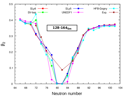
Figure 1: The Quadrupole deformation parameter $\beta_{2}$ of ${}^{124-160}\text{Nd}$ isotopes as function of their neutron number N. The experimental data are from Ref. raman2001 .

From Fig.1, we can see the $\beta_{2}$ values of our calculations are generally close to experimental ones raman2001 . On the other hand, there is an agreement between our calculations and HFB theory based on the D1S Gogny forceHFB . In the vicinity of the region where N = 82, the $\beta_{2}$ values show minima ($\beta_{2}\simeq 0$) as expected because all nuclei with the magic number N=82 are spherical. For the ${}^{140}\text{Sm}$ nucleus, we find different results between the four Skyrme forces in this study. For the Skyrme forces SLy6 and SLy5, ${}^{140}\text{Sm}$ has a triaxial shape ($\gamma\simeq 28.0^{\circ}$). It has a prolate shape for SV-bas ($\gamma=0.0^{\circ}$), and has an approximate spherical form for UNEDF1 force ($\beta_{2}\simeq 0.026$). For comparison, Calculations by Möller et al.moller2008 , based on the finite-range droplet model, predicted the ground state of ${}^{140}\text{Sm}$ nucleus to be triaxial ($\gamma=30.0^{\circ}$). In table 2, the ($\beta_{2}$,$\gamma$) values obtained in this work as well as those of HFB theory based on the D1S Gogny forceHFB and avialable experimental data raman2001 show a shape transition from spherical ${}^{144}\text{Sm}$ (N=82) to deformed shape below and above the magic neutron number N=82. For ${}^{128-144}\text{Sm}$ isotopes below N = 82, the isotopic chains exhibit a transition from prolate ($\gamma=0.0^{\circ}$) to spherical shape ($\beta_{2}\simeq 0.000$) passing through triaxial form ($22.0^{\circ}\leq\gamma\leq 28.0^{\circ}$) for ${}^{136-140}\text{Sm}$ isotopes, and for neutron number higher than N = 82, both the experimental and theoretical results show that the prolate deformation increases gradually and then saturates at a value which closes to $\beta_{2}\simeq$ 0.368.

4.2 Giant dipole resonance in ${}^{128-164}\text{Sm}$ nuclei

Based on the TDHF ground states for ${}^{128-164}\text{Sm}$ isotopes obtained in static calculations, we perform dynamic calculation such as GDR in this work to obtain some of its properties as we will see later.

4.2.1 The time evolution of the dipole moment $D_{m}(t)$

The dipole moment $D_{m}(t)$ defined by Eq. (11) allows to predict the collective motions of nucleons along the three directions x, y and z. The time evolution of $D^{i}_{m}(t)$ where i denotes x, y and z of ${}^{138}\text{Sm}$, ${}^{144}\text{Sm}$ and ${}^{154}\text{Sm}$ is plotted in Fig. 2. We note that the collective motion of nucleons in GDR is done generally along two axes. The oscillation frequency $\omega_{i}$ is related to the nuclear radius $R_{i}$ by $\omega_{i}\propto R_{i}^{-1}$ where i$\in${x,y,z}. Fig. 2(a) shows the time evolution of dipole moment for ${}^{144}\text{Sm}$ and ${}^{154}\text{Sm}$.

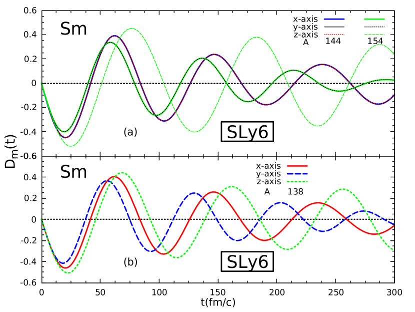
Figure 2: The dipole moment $D_{m}(t)$ as function of the simulation time t(fm/c) calculated with the Skyrme force SLy6 for ${}^{138}\text{Sm}$, ${}^{144}\text{Sm}$ and ${}^{154}\text{Sm}$.

For the ${}^{144}\text{Sm}$ nucleus, the three components $D^{x}_{m}(t)$, $D^{y}_{m}(t)$ and $D^{z}_{m}(t)$ are identical ,i.e., the oscillation frequencies along the three axes are equal ( $\omega_{x}=\omega_{y}=\omega_{z}$) which confirms that this nucleus has a spherical shape as we predicted in static calculations ($\beta_{2}\simeq 0.000$). For the ${}^{154}\text{Sm}$ nucleus, the $D^{x}_{m}(t)$ and $D^{y}_{m}(t)$ values are identical and differ from the values of $D^{z}_{m}(t)$ ,i.e., the oscillation frequencies along the symmetry z-axis $\omega_{z}$ are lower than that along the two other axes x and y which they are equal $\omega_{x}=\omega_{y}$. This confirms that ${}^{154}\text{Sm}$ has a prolate shape because $\omega_{z}<\omega_{x}=\omega_{y}$Masur2006 which is consistent with our static calculations ($\gamma=0.0^{\circ}$). We point out that we found almost the same situation for the prolate nuclei namely ${}^{130-134}\text{Sm}$ and ${}^{148-164}\text{Sm}$. In Fig. 2(b), the values of the three components $D^{i}_{m}(t)$ are different from each other in the case of the ${}^{138}\text{Sm}$ nucleus. We notice that the oscillation frequencies $\omega_{i}$ along the three axes are different from each other $\omega_{x}\neq\omega_{y}\neq\omega_{z}$ which confirms that this nucleus has a triaxial shape as we predicted in static calculations ($\gamma\simeq 25.0^{\circ}$). The same situation occurs for ${}^{136}\text{Sm}$. We note also that the time evolution of dipole moment $D_{m}(t)$ is almost the same for the others Skyrme forces (SLy5, UNEDF1, SVbas) with an exception for some nuclei as ${}^{140}\text{Sm}$. The periodicity of the three components $D^{i}_{m}(t)$ allows the excitation energies $E_{i}$ to be estimated for the oscillations along each of the three axes. For ${}^{144}\text{Sm}$, we obtain, for $D^{x}_{m}(t)$, $D^{y}_{m}(t)$ and $D^{z}_{m}(t)$, the same period T $\simeq$ 84.3 fm/c giving an excitation energy $E_{x}=E_{y}=E_{z}\simeq$ 14.70 MeV. This value is slightly lower than the experimental one $E_{GDR}^{exp.}$=15.3$\pm$ 0.1 carlos1974 . The table 3 shows the excitation energies for ${}^{138}\text{Sm}$ and ${}^{154}\text{Sm}$ nuclei with Skyrme force SLy6.

Table 3: The excitation energies along the three axes for ${}^{138}\text{Sm}$ and ${}^{154}\text{Sm}$ with Sly6, obtained from the time evolution of $D^{i}_{m}(t)$.

Nuclei		$E_{x}$(MeV)			$E_{y}$(MeV)			$E_{z}$(MeV)
${}^{138}\text{Sm}$		14.75			16.52			13.40
${}^{154}\text{Sm}$		15.62			15.62			11.90

4.2.2 GDR Spectrum

The calculation of the Fourier transform of the isovector signal D(t) allows to obtain the GDR energy spectrum. The spectral strength S(E) (12) is simply the imaginary part of the Fourier transform of D(t).

Figs. 3 - 6 display the GDR spectra in ${}^{128-164}\text{Sm}$ isotopes calculated with the four Skyrme forces, compared with the available experimental data carlos1974 . It needs to be pointed out that the experimental data for Sm isotopes from A=128 to A=142, and from A=152 to A=160, and ${}^{146}\text{Sm}$ are not yet available. The calculated GDR spectra in ${}^{144-154}\text{Sm}$ isotopes together with the available experimental data carlos1974 are shown in Fig.3. It can be seen that all four Skyrme forces give generally acceptable agreement with the experiment with a slight down-shift of the order of 0.5 MeV for SLy5, SLy6 in the case of the spherical nucleus ${}^{144}\text{Sm}$ and the weakly deformed ${}^{148-150}\text{Sm}$ nuclei , and slight up-shift ($\sim$ 0.5 MeV) for SVbas force. The agreement is better for deformed ${}^{152-154}\text{Sm}$ nuclei , where all Skyrme forces produce the deformation splitting, in which rare-earth nuclei as Samarium (Sm) with neutron number N$\approx$90 show an example of shape transitionscarlos1974 ; maruhn2005 ; benmenana2020 . For ${}^{144}\text{Sm}$ (N=82), its GDR strength has a single-humped shape. The vibrations along the three axes degenerate ,i.e., they are the same resonance energy $E_{i}$ ($E_{x}=E_{y}=E_{z}$), which confirms that this nucleus is spherical due to the relation $E_{i}\propto R_{i}^{-1}$ where i$\in${x,y,z} speth1981 . For ${}^{148}\text{Sm}$ and ${}^{150}\text{Sm}$ nuclei, the two resonance peaks move away slightly from each other but the total GDR presents one peak, so they are also weakly deformed nuclei with prolate shape. For ${}^{152}\text{Sm}$ and ${}^{154}\text{Sm}$ nuclei, the total GDR splits into two distinct peaks which confirms that these nuclei are strongly deformed with prolate shape since the oscillations along the major axis (K=0 mode) are characterized by lower frequencies than the oscillations perpendicular to this axis (K=1 mode) speth1991 .

The isotope ${}^{146}\text{Sm}$ for which we do not have experimental data, SLy6, Sly5 and SVbas give a weakly deformed nucleus ($\beta_{2}\simeq$0.06) where the resonance peaks along the major and the minor axis are very close together, whereas UNEDF1 gives an approximate spherical nucleus ($\beta_{2}\simeq$0.01). Calculations in Ref. naz2018 , based on the self-consistent Relativistic-Hartree-Bogoliubov (RHB) formalism, predicted a shape coexistence for ${}^{146}\text{Sm}$. In order to verify the shape coexistence wood1992 ; heyde2011 in ${}^{146}\text{Sm}$ nucleus, we redid the static calculations several times from different initial deformations with SLy6 force. In all cases, we obtained two minima (prolate and oblate) whose their properties are displayed in Table 4. We can see that the difference in energy between these two minima is around $\Delta$(B.E)$\simeq$ 0.07 MeV. This is a clear indication of a shape coexistence in ${}^{146}\text{Sm}$ nucleus. According to the value of deformation parameter $\gamma$, this competition of shape is between oblate ($\gamma=60^{\circ}$) and prolate ($\gamma=0^{\circ}$) shape, but the deformation is very weak ($\beta_{2}\simeq 0.05$) in both cases. Fig.4 shows the calculated GDR spectra corresponding to two minima (prolate, oblate). It confirms this suggestion: the upper panel (Fig.4(a)) shows an oblate shape for ${}^{146}\text{Sm}$ due to oscillations along the shorter axis (K=0 mode) which are characterized by higher energies than the oscillations along the axis ($\mid$K$\mid$=1 mode) perpendicular to it, while the lower panel (Fig.4(b)) shows a prolate shape for this nucleus. In both cases, the deformation splitting $\Delta$E between the two peaks is too small which confirms that this nucleus is very weakly deformed.

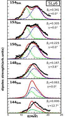
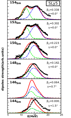
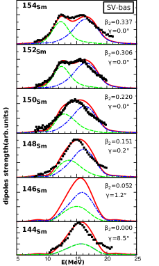
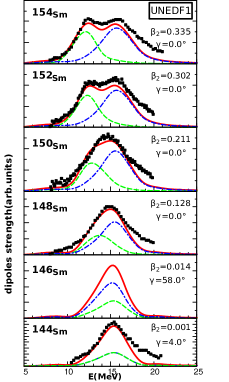
Figure 3: (Color online) GDR spectra in the chain of ${}^{144-154}\text{Sm}$ calculated with SLy6, SLy5, SVbas and UNEDF1. The solid(red), dashed(green) and dotted-dashed(blue) lines denote the dipole strengths: total, along the long axis and the short axis (multiplied by 2) respectively. The calculated strength total is compared with the experimental data carlos1974 depicted by black solid squares.

Table 4: The ground-state properties of two minima for ${}^{146}\text{Sm}$ nucleus.

Properties		Prolate minimum			Oblate minimum
Binding energy (B.E)		-1999.73 MeV			-1999.66 MeV
Root mean square (r.m.s)		4.970 fm			4.969 fm
Quadrupole deformation $\beta_{2}$		0.063			0.048
Deformation parameter $\gamma$		$0^{\circ}$			$60^{\circ}$

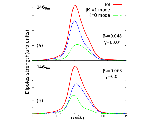
Figure 4: (Color online) The calculated GDR spectra for ${}^{146}\text{Sm}$ with the Skyrme force SLy6.

,

Fig.5 shows the GDR strength in neutron-deficient ${}^{128-142}\text{Sm}$ isotopes. We can see that the deformation decreases gradually from the well deformed nucleus ${}^{128}\text{Sm}$ ($\beta_{2}\simeq$0.4) to the approximate spherical one ${}^{142}\text{Sm}$ ($\beta_{2}\simeq$0.0) ,i.e., when the neutron number N increases and closes to the magic number N=82. We note that all Skyrme forces in this work give almost the same GDR spectra except for ${}^{140}\text{Sm}$. According to the GDR strength along the three axes, the ${}^{128}\text{Sm}$ nucleus is weakly triaxial with SLy6, SLy5 and SVbas whereas it has a prolate shape with UNEDF1. For the ${}^{130-132}\text{Sm}$ isotopes, all the four Skyrme forces predict a prolate shape for them. For ${}^{134}\text{Sm}$, SVbas and UNEDF1 predict a prolate shape, while SLy5 and SLy6 give a weak triaxial shape. For ${}^{136-138}\text{Sm}$ isotopes, we can see that the oscillations along the three axes correspond to different resonance energies $E_{i}$ ($E_{x}\neq E_{y}\neq E_{z}$), which shows that these nuclei are deformed with triaxial shape. The four Skyrme forces give different results for ${}^{140}\text{Sm}$ as displayed in Fig.5. The SLy family (SLy5 and SLy6) predict a triaxial shape, SVbas predicts a prolate shape while UNEDF1 gives an approximate spherical shape. For ${}^{142}\text{Sm}$, all Skyrme forces predict a spherical shape where the GDR strengths along the three axes are identical ,i.e., ($E_{x}=E_{y}=E_{z}$).

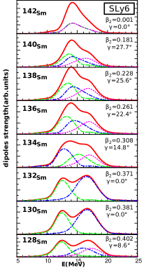
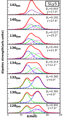
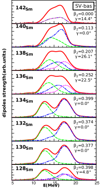
Figure 5: (Color online) GDR spectra in the isotopic chain ${}^{128-142}\text{Sm}$ calculated with SLy6, SLy5, SVbas and UNEDF1. The solid(red), dashed(green) and dotted-dashed(blue) lines denote the dipole strengths: total, along the long axis and the short axis(multiplied by 2 except ${}^{136-140}\text{Sm}$) respectively. The dotted (magenta) line denotes the strength along the third middle axis in the case of the triaxial nuclei ${}^{136-140}\text{Sm}$.

Fig.6 shows the GDR strength in neutron-rich ${}^{156-164}\text{Sm}$ isotopes. We can see that all Skyrme forces provide quite similar results. From ${}^{156}\text{Sm}$ (N=94) to ${}^{164}\text{Sm}$ (N=102), the deformation gradually gets broader, and their GDRs acquire a pronounced double-humped shape. Therefore, these nuclei are strongly deformed with prolate shape since the oscillations energies along the longer axis (z-axis) are lower than those of oscillations along the short axis (x and y axes) ,i.e., $E_{z}<E_{x}=E_{y}$.

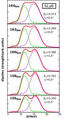
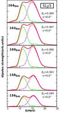
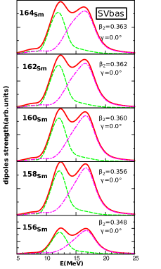
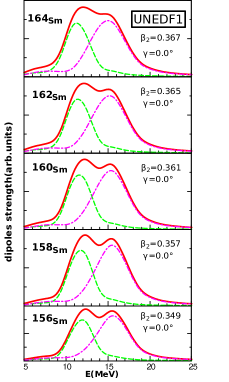
Figure 6: (color online) The GDR spectra in the isotopic chain ${}^{156-164}\text{Sm}$ calculated with SLy6, SLy5, SVbas and UNEDF1. The solid(red), dashed(green) and dotted-dashed(magenta) lines denote the dipole strengths: total, along the long axis and the short axis(multiplied by 2) respectively.

In order to compare the results between different Skyrme forces under consideration, we plot their GDR spectra into one figure, together with experimental data. Fig.7 shows the GDR strength in ${}^{144}\text{Sm}$, and ${}^{154}\text{Sm}$ calculated by the four Skyrme forces as well as the experimental data from Ref.carlos1974 . It can be seen there is a dependence of the GDR spectra on various Skyrme forces. We note a small shift of the average peak position of $\sim$ 1 MeV between these forces. The peak position of energy obtained with the Skyrme force SVbas is located highest among these four Skyrme forces. For the spherical nucleus ${}^{144}\text{Sm}$, the Skyrme force UNEDF1 reproduces well the shape and the peak among the four Skyrme forces. The agreement is less perfect with other forces. The SLy5 and SLy6 forces give very similar results, the strength exhibits a slight downshift while a slight upshift with SVbas functional. For the deformed nucleus ${}^{154}\text{Sm}$, there is an excellent agreement between the different functionals and the experiment, with a slight upshift for the K=1 mode for SVbas force. We can explain this dependence y the fact that it is linked to certain basic characteristics and nuclear properties of the Skyrme forces as shown in Table 5. The isovector effective mass $m_{1}^{*}/m$ is related to the sum rule enhancement factor $\kappa$ by $m_{1}^{*}/m=1/(1+\kappa)$ berman1975 , i.e., the larger isovector effective mass corresponds to the lighter value of the enhancement factor. We can easily see that the increase of the factor $\kappa$ (i.e., low isovector effective mass $m_{1}^{*}/m$) causes the GDR strength to shift towards the higher energy region, as indicated in Ref.nesterenko2006 for the GDR in ${}^{154}\text{Sm}$, ${}^{238}\text{U}$ and ${}^{154}\text{No}$, and in Ref.oishi2016 for ${}^{174}\text{Yb}$. For example, the large collective shift in SVbas can be related to a very high enhancement factor $\kappa$=0.4 compared to other Skyrme forces. In addition to the dependence with the enhancement factor $\kappa$, Fig.7 also shows a connection between GDR energy and symmetry energy $a_{sym}$. The peak energy of the GDR moves towards the higher energy region when $a_{sym}$ decreases, as pointed in Ref.stone2007 for the GDR in doubly magic ${}^{208}\text{Pb}$, and in our previous work for Nd isotopes benmenana2020 .

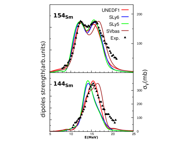
Figure 7: (Color online) The calculated GDR spectra ${}^{144}\text{Sm}$ and ${}^{154}\text{Sm}$ with Skyrme forces UNEDF1, SLy6, SLy5 and SVbas for . the experimental data carlos1974 are depicted by triangle.

Table 5: The sum rule enhancement factor $\kappa$, isovector effective mass $m_{1}^{*}/m=1/(1+\kappa)$, and symmetry energy $a_{sym}$ for the Skyrme forces under consideration.

Forces		$m_{1}^{*}/m$			$\kappa$			$a_{sym}(MeV)$
SLy6 CHABANAT1998		0.80			0.25			31.96
SLy5 CHABANAT1998		0.80			0.25			32.03
UNEDF1 kortelainen2012		$\simeq$1.00			0.001			28.98
SVbas reinhard2009		0.715			0.4			30.00

4.2.3 Relation between deformation splitting $\Delta E$ and quadrupole deformation $\beta_{2}$

As we mentioned above, the GDR strength splits into two peaks for deformed nuclei. Each peak corresponds to a resonance energy $E_{i}$ of GDR. We denoted by $E_{1}$ and $E_{2}$ the energies corresponding to K=0 and K=1 modes respectively. The total resonance energy of giant resonance is defined by the formula garg2018

$${}E_{m}=\frac{\int_{0}^{+\infty}S(E)EdE}{\int_{0}^{+\infty}S(E)dE},$$ (17)

where S(E) (12) is the strength function of giant resonance. In Table 6 , the resonance energies E₁ and E₂ of ${}^{128-164}\text{Sm}$ nuclei are presented, including the available experimental data from Ref.carlos1974 . From this table, we can see an overall agreement between our results and the experimental data, with a slightly advantage for the Sly6 functional. For instance, the result of the semi-spherical ${}^{144}\text{Sm}$ gives $E_{GDR}^{SLy6}$=15.05 MeV which is very close to $E_{GDR}^{Exp.}$=(15.30 $\pm$ 0.10) MeV. Also for deformed nuclei as ${}^{152}\text{Sm}$ and ${}^{154}\text{Sm}$, the results ($E_{1},E_{2}$) with SLy6 are very close to those of experiment.

Table 6: The resonance energy centroids $E_{1}$ and $E_{2}$ of ${}^{128-164}\text{Sm}$ corresponding to oscillation along the major axis (K=0) and the minor axis (K=1) respectively. The experimental data are from ref. carlos1974 .

	UNEDF1		SVBas		SLy5		SLy6		Exp.carlos1971
Nuclei	E1	E2	E1	E2	E1	E2	E1	E2	E1	E2
${}^{\textbf{128}}\textbf{Sm}$	13.36	17.79	13.36	17.75	12.54	16.61	12.76	16.90	—	—
${}^{\textbf{130}}\textbf{Sm}$	13.32	17.68	13.46	17.64	12.58	16.49	12.82	16.76	—	—
${}^{\textbf{132}}\textbf{Sm}$	13.15	17.59	13.47	17.55	12.63	16.46	12.89	16.69	—	—
${}^{\textbf{134}}\textbf{Sm}$	13.22	17.43	13.22	17.60	12.96	16.13	13.22	16.35	—	—
${}^{\textbf{136}}\textbf{Sm}$	14.00	16.84	14.20	16.91	13.27	15.87	13.50	16.11	—	—
${}^{\textbf{138}}\textbf{Sm}$	14.34	16.51	14.47	16.66	13.48	15.70	13.70	15.95	—	—
${}^{\textbf{140}}\textbf{Sm}$	15.42	15.73	14.93	16.25	13.73	15.50	13.95	15.72	—	—
${}^{\textbf{142}}\textbf{Sm}$	15.59	15.59	15.78	15.78	14.80	14.83	15.03	15.04	—	—
${}^{\textbf{144}}\textbf{Sm}$	15.57	15.57	15.79	15.79	14.84	14.84	15.05	15.05	15.30$\pm$ 0.1	—
${}^{\textbf{146}}\textbf{Sm}$	15.27	15.45	15.45	15.85	14.15	14.95	14.34	15.16	—	—
${}^{\textbf{148}}\textbf{Sm}$	14.07	15.69	14.25	16.15	13.34	15.24	14.29	15.47	14.80$\pm$ 0.1	—
${}^{\textbf{150}}\textbf{Sm}$	13.40	15.86	13.62	16.31	12.91	15.38	13.06	15.59	14.60$\pm$ 0.1	—
${}^{\textbf{152}}\textbf{Sm}$	12.80	16.07	13.14	16.65	12.46	15.62	12.60	15.82	12.45$\pm$ 0.1	15.85$\pm$ 0.1
${}^{\textbf{154}}\textbf{Sm}$	12.53	16.06	12.93	16.98	12.23	15.70	12.37	15.91	12.35$\pm$ 0.1	16.10$\pm$ 0.1
${}^{\textbf{156}}\textbf{Sm}$	12.36	15.97	12.80	16.55	12.12	15.64	12.26	15.82	—	—
${}^{\textbf{158}}\textbf{Sm}$	12.22	15.84	12.69	16.47	12.01	15.60	12.15	15.77	—	—
${}^{\textbf{160}}\textbf{Sm}$	12.08	15.69	12.35	16.37	11.87	15.51	12.07	15.69	—	—
${}^{\textbf{162}}\textbf{Sm}$	11.96	15.53	12.52	16.26	11.87	15.40	11.99	15.57	—	—
${}^{\textbf{164}}\textbf{Sm}$	11.84	15.37	12.44	16.14	11.82	15.33	11.95	15.50	—	—

Fig. 8 displays the resonance energies ($E_{1}$, $E_{2}$) evolution as function of the neutron number N from ${}^{128}\text{Sm}$ (N=66) to ${}^{164}\text{Sm}$ (N=102). We can see for all the four Skyrme forces that the resonance energy $E_{1}$ along the major axis (k=0 mode) increases with the neutron number N (i.e., mass number A) until the region around N=82 (magic number) and then trends to decreases. The opposite happens for the resonance energy $E_{2}$, i.e., it decreases with the increasing of N until N=82 , and then gradually increases. We can clearly see that the SLy6 reproduces the experimental data best among the four Skyrme forces. It was shown to provide a satisfying description of the GDR for spherical and deformed nuclei nesterenko2008 ; reinhard2008 . The SVbas functional gives somewhat high values of $E_{1}$ and $E_{2}$ among the other forces due to its large enhancement factor $\kappa$ ($\kappa$=0.4) as we discussed above.

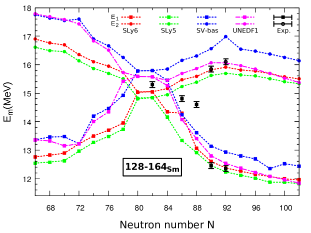
Figure 8: (Color online) The peak positions $E_{1}$ and $E_{2}$ of GDR in ${}^{128-164}\text{Sm}$ along major axis (square symbol) and minor axis (circle symbol) respectively. The experimental data are depicted by black square ($E_{1}$) and circle ($E_{2}$).

In Fig. 9, we plotted the evolution of the GDR-splitting value $\Delta E=E_{2}-E_{1}$ as a function of the neutron number N. It can be easily seen for all the four Skyrme forces, that the GDR splitting $\Delta$E decreases gradually with the increase of N and then increases. It takes the minimum value $\Delta E$=0 at N=82 (magic Number ) which corresponds to the spherical nucleus ${}^{144}\text{Sm}$ and achieves a maximum for strongly deformed nuclei as ${}^{164}\text{Sm}$. Such a result confirms that the splitting of GDR is related to the deformation structure of nuclei.

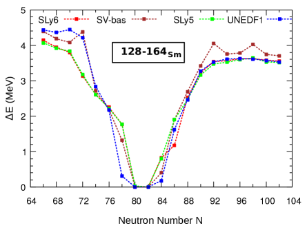
Figure 9: (Color online) The GDR-splitting $\Delta E$ as a function of the neutron number N for ${}^{128-164}\text{Sm}$ nuclei calculated with SLy6, SVbas, SLy5 and UNEDF1.

Since the GDR-splitting is caused by the deformation, it is possible to relate the nuclear deformation parameter $\beta_{2}$ with the ratio $\Delta E/\bar{E}$, where $\bar{E}$ is the mean resonance energy. Fig. 10 displays the correlation between the quadrupole deformation $\beta_{2}$ and $\Delta E/\bar{E}$ for ${}^{128-164}\text{Sm}$ nuclei calculated with the Skyrme forces under consideration. We can see for all of the four Skyrme forces that there is an almost linear relationship between $\Delta E/\bar{E}$ and $\beta_{2}$, i.e.,

$${}\Delta E/\bar{E}\simeq a.\beta_{2},$$ (18)

where a is a parameter depending slightly on the Skyrme force. This fact confirms that the size of the GDR-splitting is proportional to the quadrupole deformation parameter $\beta_{2}$. The relation (18) was already studied in Refs. okamoto1958 ; ring2009 ; benmenana2020 .

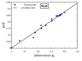
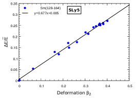
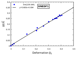
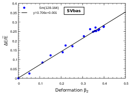
Figure 10: (Color online) The correlation between the deformation parameter $\beta_{2}$ and the ratio $\Delta E/\bar{E}$. circles denote the data in the Sm isotopes and lines are the fitting results.

5 Conclusion

The isovector giant dipole resonance (IVGDR) has been investigated in the isotopic chain of Samarium (Sm). The study covers even-even Sm isotopes from ${}^{128}\text{Sm}$ to ${}^{164}\text{Sm}$. The investigations have been done within the framework of time dependent Hartree-Fock (TDHF) method based on the Skyrme functional. The calculations were performed with Four Skyrme forces: SLy6, SLy5, SVbas and UNEDF1. In static calculations, some properties of ground state like the deformation parameters ($\beta_{2},\gamma$) have been calculated by using SKY3D code sky3d . In dynamic calculations, the dipole moment D_m(t) and the strength of GDR are calculated and compared with the available experimental data carlos1974 . The results obtained showed that TDHF method can reproduce the shape and the peak of the GDR spectra. All four Skyrme forces generally reproduce the average position of the GDR strength with a small shift depending on the used Skyrme force. The agreement is better with the SLy6 force among these Skyrme forces. The GDR strengths in ${}^{128-142}\text{Sm}$, ${}^{146}\text{Sm}$ and ${}^{156-164}\text{Sm}$ nuclei are also predicted in this work.

Finally, some properties of GDR ($\bar{E}$, $E_{1}$, $E_{2}$, $\Delta E$ ) have been calculated with the four Skyrme forces. The results with SLy6 were very close to the experimental data compared to the other forces. A correlation between the ratio $\Delta E/\bar{E}$ and the quadrupole deformation parameter $\beta_{2}$ was found. For all Skyrme forces, we have found the relation $\Delta E/\bar{E}=a.\beta_{2}+b$ with the value of b is negligible.

In the light of the successful description of the GDR in deformed nuclei with the TDHF method, it was expected that this latter can also be applied for treating the shape coexistence as we predicted for ${}^{146}\text{Sm}$ with the SLy6 force.

References

- (1) M. N. Harakeh and A. Woude, Giant Resonances: fundamental high-frequency modes of nuclear excitation, vol. 24. Oxford University Press on Demand, (2001).
- (2) M. Goldhaber and E. Teller Phys. Rev., vol. 74, p. 1046, (1948).
- (3) J. Speth and A. van der Woude Reports on Progress in Physics, vol. 44, p. 719, (1981).
- (4) B. L. Berman and S. Fultz Reviews of Modern Physics, vol. 47, p. 713, (1975).
- (5) W. Bothe and W. Gentner Z.Phys, vol. 106, p. 236, (1937).
- (6) P. Carlos, H. Beil, R. Bergere, A. Lepretre, and A. Veyssiere Nuclear Physics A, vol. 172, p. 437, (1971).
- (7) P. Carlos, H. Beil, R. Bergere, A. Lepretre, A. De Miniac, and A. Veyssiere Nuclear Physics A, vol. 225, p. 171, (1974).
- (8) L. Donaldson, C. Bertulani, J. Carter, and al. Physics Letters B, vol. 776, p. 133, (2018).
- (9) K. Goeke and J. Speth Annual Review of Nuclear and Particle Science, vol. 32, p. 65, (1982).
- (10) J. A. Maruhn, P. G. Reinhard, P. D. Stevenson, J. R. Stone, and M. R. Strayer Phys. Rev. C, vol. 71, p. 064328, (2005).
- (11) W. Kleinig, V. O. Nesterenko, J. Kvasil, P.-G. Reinhard, and P. Vesely Phys. Rev. C, vol. 78, p. 044313, (2008).
- (12) K. Yoshida and T. Nakatsukasa Phys. Rev. C, vol. 83, p. 021304, (2011).
- (13) A. A. B. Mennana, Y. E. Bassem, and M. Oulne Physica Scripta, vol. 95, p. 065301, 2020.
- (14) S. Josef, Electric and magnetic giant resonances in nuclei, vol. 7. World Scientific, (1991).
- (15) V. Nesterenko, W. Kleinig, J. Kvasil, P. Vesely, and P.-G. Reinhard International Journal of Modern Physics E, vol. 16, p. 624, (2007).
- (16) S. Fracasso, E. B. Suckling, and P. Stevenson Physical Review C, vol. 86, p. 044303, (2012).
- (17) D. P. n. Arteaga, E. Khan, and P. Ring Phys. Rev. C, vol. 79, p. 034311, (2009).
- (18) S. S. Wang, Y. G. Ma, X. G. Cao, W. B. He, H. Y. Kong, and C. W. Ma Phys. Rev. C, vol. 95, p. 054615, (2017).
- (19) V. M. Masur and L. M. Mel’nikova Physics of Particles and Nuclei, vol. 37, p. 923, (2006).
- (20) E. Ramakrishnan, T. Baumann, and al. Physical review letters, vol. 76, p. 2025, (1996).
- (21) J. Gundlach, K. Snover, J. Behr, and al. Physical review letters, vol. 65, p. 2523, (1990).
- (22) P. A. M. Dirac Mathematical Proceedings of the Cambridge Philosophical Society, vol. 26, p. 376, (1930).
- (23) J. Błocki and H. Flocard Physics Letters B, vol. 85, p. 163, (1979).
- (24) P. Chomaz, N. Van Giai, and S. Stringari Physics Letters B, vol. 189, p. 375, (1987).
- (25) J. A. Maruhn, P.-G. Reinhard, P. D. Stevenson, and M. R. Strayer Phys. Rev. C, vol. 74, p. 027601, (2006).
- (26) P. Stevenson, M. Strayer, J. Rikovska Stone, and W. Newton International Journal of Modern Physics E, vol. 13, p. 181, (2004).
- (27) B. Schuetrumpf, P.-G. Reinhard, P. Stevenson, A. Umar, and J. Maruhn Computer Physics Communications, vol. 229, p. 211, (2018).
- (28) E. Chabanat, P. Bonche, P. Haensel, J. Meyer, and R. Schaeffer Nuclear Physics A, vol. 635, p. 231, (1998).
- (29) P. Klüpfel, P.-G. Reinhard, T. J. Bürvenich, and J. A. Maruhn Phys. Rev. C, vol. 79, p. 034310, (2009).
- (30) M. Kortelainen, J. McDonnell, W. Nazarewicz, P.-G. Reinhard, J. Sarich, N. Schunck, M. V. Stoitsov, and S. M. Wild Phys. Rev. C, vol. 85, p. 024304, (2012).
- (31) C. Tao, Y. Ma, G. Zhang, X. Cao, D. Fang, H. Wang, et al. Physical Review C, vol. 87, no. 1, p. 014621, 2013.
- (32) N. Paar, D. Vretenar, E. Khan, and G. Colo Reports on Progress in Physics, vol. 70, no. 5, p. 691, 2007.
- (33) J. W. Negele Reviews of Modern Physics, vol. 54, p. 913, (1982).
- (34) Y. Engel, D. Brink, K. Goeke, S. Krieger, and D. Vautherin Nuclear Physics A, vol. 249, p. 215, (1975).
- (35) A. Kerman and S. Koonin Annals of Physics, vol. 100, p. 332, (1976).
- (36) S. E. Koonin, K. T. R. Davies, V. Maruhn-Rezwani, H. Feldmeier, S. J. Krieger, and J. W. Negele Phys. Rev. C, vol. 15, p. 1359, (1977).
- (37) P.-G. Reinhard, L. Guo, and J. Maruhn The European Physical Journal A, vol. 32, p. 19, (2007).
- (38) C. Simenel and A. Umar Progress in Particle and Nuclear Physics, vol. 103, p. 19, (2018).
- (39) C. Simenel The European Physical Journal A, vol. 48, p. 152, (2012).
- (40) H. Flocard, S. E. Koonin, and M. S. Weiss Phys. Rev. C, vol. 17, p. 1682, (1978).
- (41) P. Bonche, S. Koonin, and J. W. Negele Phys. Rev. C, vol. 13, p. 1226, (1976).
- (42) T. Skyrme Nuclear Physics, vol. 9, p. 615, (1958).
- (43) C. Simenel and P. Chomaz Phys. Rev. C, vol. 80, p. 064309, (2009).
- (44) J. M. Broomfield and P. D. Stevenson Journal of Physics G: Nuclear and Particle Physics, vol. 35, p. 095102, (2008).
- (45) P. Ring and P. Schuck, The nuclear many-body problem. Springer-Verlag, (1980).
- (46) P.-G. Reinhard, P. D. Stevenson, D. Almehed, J. A. Maruhn, and M. R. Strayer Phys. Rev. E, vol. 73, p. 036709, (2006).
- (47) J. Meng, W. Zhang, S. Zhou, H. Toki, and L. Geng The European Physical Journal A-Hadrons and Nuclei, vol. 25, p. 23, (2005).
- (48) T. Naz, G. Bhat, S. Jehangir, S. Ahmad, and J. Sheikh Nuclear Physics A, vol. 979, p. 1, (2018).
- (49) K. W. N. Takigawa, ”Fundamentals of Nuclear Physics”. Springer Japan, (2017).
- (50) S. RAMAN, C. NESTOR, and P. TIKKANEN Atomic Data and Nuclear Data Tables, vol. 78, p. 1, (2001).
- (51) J.-P. Delaroche, M. Girod, J. Libert, H. Goutte, S. Hilaire, S. Péru, N. Pillet, and G. Bertsch Physical Review C, vol. 81, p. 014303, (2010).
- (52) P. Möller, R. Bengtsson, B. Carlsson, P. Olivius, T. Ichikawa, H. Sagawa, and A. Iwamoto Atomic Data and Nuclear Data Tables, vol. 94, p. 758, (2008).
- (53) J. Wood, K. Heyde, W. Nazarewicz, M. Huyse, and P. Van Duppen Physics reports, vol. 215, p. 101, (1992).
- (54) K. Heyde and J. L. Wood Reviews of Modern Physics, vol. 83, p. 1467, (2011).
- (55) V. Nesterenko, W. Kleinig, J. Kvasil, P. Vesely, P.-G. Reinhard, and D. Dolci Physical Review C, vol. 74, p. 064306, (2006).
- (56) T. Oishi, M. Kortelainen, and N. Hinohara Phys. Rev. C, vol. 93, p. 034329, (2016).
- (57) J. R. Stone and P.-G. Reinhard Progress in Particle and Nuclear Physics, vol. 58, p. 587, (2007).
- (58) U. Garg and G. Colò Progress in Particle and Nuclear Physics, vol. 101, p. 55, (2018).
- (59) V. Nesterenko, W. Kleinig, J. Kvasil, P. Vesely, and P.-G. Reinhard International Journal of Modern Physics E, vol. 17, p. 89, (2008).
- (60) K. Okamoto Phys. Rev., vol. 110, p. 143, (1958).