A solution to the fifth and the eighth Busemann-Petty problems in a small neighborhood of the Euclidean ball

Abstract.

We show that the fifth and the eighth Busemann-Petty problems have positive solutions for bodies that are sufficiently close to the Euclidean ball in the Banach-Mazur distance.

1. Introduction

In 1956, Busemann and Petty [BP] posed ten problems about symmetric convex bodies, of which only the first one has been solved (see [K]). Their fifth and eighth problems are as follows.

Problem 5.

If for an origin-symmetric convex body $K\subset{\mathbb{R}^{n}}$, $n\geq 3$, we have

(1) $$h_{K}(\theta)\textnormal{vol}_{n-1}(K\cap\theta^{\perp})=C\qquad\forall\theta\in S^{n-1},$$

where the constant $C$ is independent of $\theta$, must $K$ be an ellipsoid?

Here $S^{n-1}$ is the unit sphere in $\mathbb{R}^{n}$, $\theta^{\perp}=\{x\in{\mathbb{R}^{n}}:\langle x,\theta\rangle=0\}$ is the hyperplane orthogonal to the direction $\theta\in S^{n-1}$ and passing through the origin, and $h_{K}(\theta)=\max\limits_{x\in K}\langle x,\theta\rangle$ is the support function of the convex body $K\subset{\mathbb{R}^{n}}$.

Problem 8.

If for an origin-symmetric convex body $K\subset{\mathbb{R}^{n}}$, $n\geq 3$, we have

(2) $$f_{K}(\theta)=C(\textnormal{vol}_{n-1}(K\cap\theta^{\perp}))^{n+1}\qquad\forall\theta\in S^{n-1},$$

where the constant $C$ is independent of $\theta$, must $K$ be an ellipsoid?

Here $f_{K}$ is the curvature function of $K$, which is the reciprocal of the Gaussian curvature viewed as a function of the unit normal vector (see [Sch, pg. 419]).

The Euclidean ball clearly satisfies (1) and (2). If a body $K$ satisfies (1), then so does $TK$ for any linear transformation $T\in GL(n)$ (with constant $C\cdot|\det T|$). Similarly, if a body $K$ satisfies (2), then so does $TK$ for any linear transformation $T\in GL(n)$ (with constant $C\cdot|\det T|^{1-n}$). Hence, (1) and (2) are satisfied by ellipsoids.

In this paper we prove the following result.

Theorem.

Let $n\geq 3$. If an origin-symmetric convex body $K\subset{\mathbb{R}^{n}}$ satisfies (1) or (2) and is sufficiently close to the Euclidean ball in the Banach-Mazur metric, then $K$ must be an ellipsoid.

In dimension 2, there are convex bodies satisfying (1) that are not ellipses but, nevertheless, can be arbitrarily close to the unit disc. The curve bounding such a body is a so-called Radon curve, see [D]. On the other hand, the only convex bodies satisfying (2) in dimension 2 are the ellipses [P, Theorem 5.6].

2. Invariance of Busemann-Petty problems under linear transformations

Both Busemann-Petty problems are invariant under linear transformations in the sense that if a symmetric convex body $K$ satisfies (1) or (2), then so does $TK$ where $T$ is an invertible linear map from ${\mathbb{R}^{n}}$ to itself.

This statement is almost obvious for Problem 5. Indeed, let $H$ be any hyperplane in ${\mathbb{R}^{n}}$ passing through the origin and let $H_{s}$ be a support hyperplane of $K$ parallel to $H$. Consider any point $p\in K\cap H_{s}$ and the cone $C_{K,H}$ with the base $K\cap H$ and the vertex $p$. Note that due to the symmetry of $K$ and the fact that $H_{s}$ is parallel to $H$, the volume $\textrm{vol}_{n}(C_{K,H})$ of this cone is independent of the particular choice of $H_{s}$ and $p$. Moreover, we clearly have $C_{TK,TH}=T(C_{K,H})$, so $\textrm{vol}_{n}(C_{TK,TH})=|\det T|\textrm{vol}_{n}(C_{K,H})$. Since for $H=\theta^{\perp}$ this volume can be expressed as $\textrm{vol}_{n}(C_{K,H})=\frac{1}{n}\textrm{vol}_{n-1}(K\cap\theta^{\perp})h_{K}(\theta)$, we see that property (1) is merely the statement that $\textrm{vol}_{n}(C_{K,H})$ is independent of the choice of the hyperplane $H$ (this was exactly how the fifth Busemann-Petty problem was originally formulated in [BP]).

The invariance of (2) under linear transformations is somewhat less transparent. When $K$ has smooth non-degenerate $C^{2}$-boundary with strictly positive Gaussian curvature at each point, we can restate it as follows.

Let, as before, $H$ be an arbitrary hyperplane passing through the origin, let $H_{s}$ be one of the two supporting hyperplanes of $K$ parallel to $H$, and let $p\in K\cap H_{s}$. For $t\in(0,1)$, let $H^{t}$ be the hyperplane between $H$ and $H_{s}$ parallel to $H$ such that the distance between $H_{s}$ and $H^{t}$ is $t$ times the distance $d$ between $H_{s}$ and $H$. Then, for small $t$, the $(n-1)$-dimensional volume $\textrm{vol}_{n-1}(K\cap H^{t})$ is approximately proportial to $\frac{t^{\frac{n-1}{2}}d^{\frac{n-1}{2}}}{\sqrt{G(p)}}$ where $G(p)$ is the Gaussian curvature of $\partial K$ at $p$.

Note now that $\frac{\textrm{vol}_{n-1}(K\cap H^{t})}{\textrm{vol}_{n-1}(K\cap H)}$ is invariant under linear transformations and $d\,\textrm{vol}_{n-1}(K\cap H)=n\,\textrm{vol}_{n}(C_{K,H})$ is multiplied by $|\det T|$ when we replace $K$ by $TK$ and $H$ by $TH$. Thus, $G(p)\textrm{vol}_{n-1}(K\cap H)^{n+1}$ equals (up to a constant factor depending on the dimension $n$ only)

$$\lim\limits_{t\to 0}t^{n-1}\textrm{vol}_{n}(C_{K,H})^{n-1}\Big{[}\frac{\textrm{vol}_{n-1}(K\cap H)}{\textrm{vol}_{n-1}(K\cap H^{t})}\Big{]}^{2},$$

and thus is multiplied by $|\det T|^{n-1}$ when we replace $K$ by $TK$ and $H$ by $TH$.

In general, it is unclear to us what degree of smoothness Busemann and Petty assumed when posing Problem 8. We will handle the most general case, when (2) is understood in the sense that the surface area measure of $K$ is absolutely continuous with respect to the $(n-1)$-dimensional Lebesgue measure on the unit sphere and its Radon-Nikodym density is equal to the right-hand side. In this case, the geometric meaning of (2) is less transparent but the invariance of (2) under linear transformations still follows from the computations in [Lu]. The reader will lose almost nothing, however, by assuming that $\partial K$ is smooth and non-degenerate, but $K$ is close to the unit ball only in the Banach-Mazur distance and not in $C^{2}$.

3. From the Banach-Mazur distance to the Hausdorff one

Applying an appropriate linear transformation, we can assume that the constants in (1) and (2) are equal to those for the unit ball $B^{n}_{2}$ and that $(1-\varepsilon)rB^{n}_{2}\subset K\subset(1+\varepsilon)rB^{n}_{2}$ for some $r>0$ with some small $\varepsilon>0$.

Our task here will be to show that $r$ must be close to $1$, i.e., $K$ must be close to the unit Euclidean ball $B^{n}_{2}$ in the Hausdorff metric. We have

(3) $$(1-\varepsilon)rh_{B^{n}_{2}}\leq h_{K}\leq(1+\varepsilon)rh_{B^{n}_{2}}$$

and

(4) $$(1-\varepsilon)^{n-1}r^{n-1}\textrm{vol}_{n-1}(B^{n}_{2}\cap\theta^{\perp})\leq\textrm{vol}_{n-1}(K\cap\theta^{\perp})\leq$$

$$(1+\varepsilon)^{n-1}r^{n-1}\textrm{vol}_{n-1}(B^{n}_{2}\cap\theta^{\perp}).$$

In the case of (1), combining (3) and (4) with the equation

$$h_{K}(\theta)\textrm{vol}_{n-1}(K\cap\theta^{\perp})=h_{B^{n}_{2}}(\theta)\textrm{vol}_{n-1}(B^{n}_{2}\cap\theta^{\perp}),$$

we obtain $(1-\varepsilon)^{n}r^{n}\leq 1\leq(1+\varepsilon)^{n}r^{n}$, i.e., $\frac{1}{1+\varepsilon}\leq r\leq\frac{1}{1-\varepsilon}$.

In the case of (2), we can integrate both sides with respect to the $(n-1)$-dimensional Lebesgue measure on $S^{n-1}$ to conclude (see [Sch], Section 5.3.1) that

(5) $$\Sigma(K)=\int_{S^{n-1}}f_{K}(\theta)dm_{n-1}(\theta)=$$

$$c_{n}\int_{S^{n-1}}\left(\textrm{vol}_{n-1}(K\cap\theta^{\perp})\right)^{n+1}dm_{n-1}(\theta),$$

where $\Sigma(K)$ is the surface area of $\partial K$ and $c_{n}$ is defined by

$$\Sigma(B^{n}_{2})=c_{n}\int_{S^{n-1}}\left(\textrm{vol}_{n-1}(B^{n}_{2}\cap\theta^{\perp})\right)^{n+1}dm_{n-1}(\theta).$$

From our assumption $(1-\varepsilon)rB^{n}_{2}\subset K\subset(1+\varepsilon)rB^{n}_{2}$, it follows that

$$(1-\varepsilon)^{n-1}r^{n-1}\Sigma(B^{n}_{2})\leq\Sigma(K)\leq(1+\varepsilon)^{n-1}r^{n-1}\Sigma(B^{n}_{2}),$$

which, together with (4) and (5), gives

$$(1-\varepsilon)^{n-1}r^{n-1}\leq(1+\varepsilon)^{(n-1)(n+1)}r^{(n-1)(n+1)}$$

and

$$(1+\varepsilon)^{n-1}r^{n-1}\geq(1-\varepsilon)^{(n-1)(n+1)}r^{(n-1)(n+1)},$$

i.e.,

$$\frac{1-\varepsilon}{(1+\varepsilon)^{n+1}}\leq r^{n}\leq\frac{1+\varepsilon}{(1-\varepsilon)^{n+1}}.$$

4. The isotropic position

We have seen in the previous section that, without loss of generality, we may assume that $(1-\varepsilon)B^{n}_{2}\subset K\subset(1+\varepsilon)B^{n}_{2}$. However, this requirement still leaves some freedom as to what affine image of $K$ to choose. In this section we will reduce this freedom even further by putting $K$ into the so-called isotropic position, i.e., the position where

$$\int_{K}\langle x,y\rangle^{2}dy=c\,|x|^{2}\qquad\qquad\forall x\in{\mathbb{R}^{n}}.$$

The existence of such a position is well known and easy to derive (see [BGVV], Section 2.3.2). Indeed, for an arbitrary symmetric convex body $K$, the mapping

$${\mathbb{R}^{n}}\ni x\,\mapsto\int_{K}\langle x,y\rangle^{2}dy=\sum\limits_{i,j}\Big{(}\int_{K}y_{i}y_{j}dy\Big{)}x_{i}x_{j}$$

is a positive-definite quadratic form. Thus, it can be written as $\langle Sx,x\rangle$, where $S$ is a self-adjoint positive definite operator on ${\mathbb{R}^{n}}$.

Moreover, if $K=B^{n}_{2}$, then $S=c_{n}I$ for some $c_{n}>0$. If $(1-\varepsilon)B^{n}_{2}\subset K$, then

$$\langle Sx,x\rangle=\int_{K}\langle x,y\rangle^{2}dy\geq\int_{(1-\varepsilon)B^{n}_{2}}\langle x,y\rangle^{2}dy=(1-\varepsilon)^{n+2}c_{n}|x|^{2}$$

and, similarly, if $K\subset(1+\varepsilon)B^{n}_{2}$, then

$$\langle Sx,x\rangle\leq(1+\varepsilon)^{n+2}c_{n}|x|^{2}.$$

Thus, setting $\widetilde{S}=c_{n}^{-1}S$, we have

$$(1-\varepsilon)^{n+2}|x|^{2}\leq\langle\widetilde{S}x,x\rangle\leq(1+\varepsilon)^{n+2}|x|^{2}.$$

It follows that

$$(1-\varepsilon)^{n(n+2)}\leq\det(\widetilde{S})\leq(1+\varepsilon)^{n(n+2)}$$

and

$$\|\widetilde{S}\|\leq(1+\varepsilon)^{n+2},\quad\|\widetilde{S}^{-1}\|\leq(1-\varepsilon)^{-(n+2)},$$

whence the operator $T=\sqrt{\det(\widetilde{S})^{-\frac{1}{n}}\widetilde{S}}$ satisfies

$$\det T=1,\qquad\qquad\|T\|,\,\|T^{-1}\|\leq\Big{(}\frac{1+\varepsilon}{1-\varepsilon}\Big{)}^{\frac{n+2}{2}},$$

and $T^{-1}ST^{-1}$ is a multiple of the identity.

The body $\widetilde{K}=T^{-1}K$ satisfies

$$\int_{\widetilde{K}}\langle x,y\rangle^{2}dy=\int_{K}\langle x,T^{-1}y\rangle^{2}dy=\int_{K}\langle T^{-1}x,y\rangle^{2}dy=$$

$$\langle ST^{-1}x,T^{-1}x\rangle=\langle T^{-1}ST^{-1}x,x\rangle=c|x|^{2}$$

for some $c>0$, while we also have

$$(1-\varepsilon)\Big{(}\frac{1-\varepsilon}{1+\varepsilon}\Big{)}^{\frac{n+2}{2}}B^{n}_{2}\subset T^{-1}(1-\varepsilon)B^{n}_{2}\subset T^{-1}K$$

$$\subset T^{-1}(1+\varepsilon)B^{n}_{2}\subset(1+\varepsilon)\Big{(}\frac{1+\varepsilon}{1-\varepsilon}\Big{)}^{\frac{n+2}{2}}B^{n}_{2}.$$

5. The analytic reformulation

Let $\rho_{K}$, $h_{K}:S^{n-1}\to{\mathbb{R}}$ be the radial and the support functions of the convex body $K$ respectively, i.e.,

$$\rho_{K}(\theta)=\max\{t>0:\,t\theta\in K\}$$

and

$$h_{K}(\theta)=\max\{\langle x,\theta\rangle:\,x\in K\}.$$

The $(n-1)$-dimensional volume of the section $K\cap\theta^{\perp}$ is given by

$$\textrm{vol}_{n-1}(K\cap\theta^{\perp})=c_{n}\mathcal{R}\Big{[}\rho_{K}^{n-1}\Big{]},$$

where $c_{n}$ is a positive constant depending on the dimension $n$ only and $\mathcal{R}$ is the Radon transform on $S^{n-1}$, i.e.,

$$\mathcal{R}f(\theta)=\int_{S^{n-1}\cap\theta^{\perp}}f(\xi)d\sigma(\xi)$$

with $\sigma$ being the $(n-2)$-dimensional Lebesgue measure on $S^{n-1}\cap\theta^{\perp}$ normalized by the condition $\sigma(S^{n-1}\cap\theta^{\perp})=1$, i.e., $\mathcal{R}1=1$. Thus, condition (1) can be rewritten as $h_{K}\mathcal{R}\Big{[}\rho_{K}^{n-1}\Big{]}=C$, where, due to the normalization made at the beginning of Section 3, the constant $C$ should be the same as for the unit ball $B^{n}_{2}$, i.e., $C=1$. So, we arrive at the equation

(6) $$h_{K}=\Big{(}\mathcal{R}\Big{[}\rho_{K}^{n-1}\Big{]}\Big{)}^{-1}.$$

Rewriting (2) in terms of $h_{K}$ and $\rho_{K}$ is trickier. The right-hand side presents no problem: it is just proportional to $\Big{(}\mathcal{R}\Big{[}\rho_{K}^{n-1}\Big{]}\Big{)}^{n+1}$. So, the equation becomes $f_{K}=C\Big{(}\mathcal{R}\Big{[}\rho_{K}^{n-1}\Big{]}\Big{)}^{n+1}$. Due to the normalization made at the beginning of Section 3, the constant $C$ should be the same as for the unit ball $B^{n}_{2}$, i.e., $C=1$. However, $f_{K}$ can be readily expressed in terms of $h_{K}$ only if $h_{K}$ is $C^{2}$ and we have made no such assumption.

The expression for $f_{K}$ in the $C^{2}$-case can be written as $f_{K}=Ah_{K}$ where the operator $A$ is defined as follows. For a function $h\in C^{2}(S^{n-1})$ denote by $H(x)$ its degree $1$ homogeneous extension to the entire space (i.e., $H(x)=|x|h(\frac{x}{|x|})$ for $x\neq 0$). Let $\widehat{H}=(H_{x_{i}x_{j}})_{i,j=1}^{n}$ be the Hessian of $H$ and let $\widehat{H}_{j}$ be the matrix obtained from $H$ by removing the $j$-th row and the $j$-th column. Let $Ah$ be the restriction of $\sum\limits_{j=1}^{n}\det\widehat{H}_{j}$ to the unit sphere $S^{n-1}$ (see [Sch], Corollary 2.5.3).

We shall show that when $\rho_{K}$ is close to $1$, we can solve the equation

$$Ah=\Big{(}\mathcal{R}\Big{[}\rho_{K}^{n-1}\Big{]}\Big{)}^{n+1}$$

with $h$ close to $1$ in $C^{2}$. This $h$ will determine a convex body $L$ that satisfies $f_{L}=f_{K}$. By the uniqueness theorem (see [Sch], Theorem 8.1.1) we will then conclude that $K=L$, so $h_{K}=h$ and the smoothness of $h_{K}$ will be justified a posteriori. Thus, it will be possible to rewrite (2) as

(7) $$Ah_{K}=\Big{(}\mathcal{R}\Big{[}\rho_{K}^{n-1}\Big{]}\Big{)}^{n+1}.$$

6. Maximal function

For $e\in S^{n-1}$, $\vartheta\in(0,\pi]$, let $S_{\vartheta}(e)=\{e^{\prime}\in S^{n-1},\,\langle e,e^{\prime}\rangle\geq\cos\vartheta\}$ denote the spherical cap centered at $e$ with spherical radius $\vartheta$. The spherical Hardy-Littlewood maximal function is defined by

$$Mf(e)=\max\limits_{\vartheta\in(0,\pi]}\frac{1}{\sigma(S_{\vartheta}(e))}\int_{S_{\vartheta}(e)}|f(x)|d\sigma(x),\qquad f\in L^{1}(S^{n-1}),$$

where $\sigma$ is the surface measure on $S^{n-1}$ normalized by the condition $\sigma(S^{n-1})$ $=1$. It is well known that $M$ is bounded as an operator from $L^{2}(S^{n-1})$ to itself (see [Kn]).

Lemma 1.

Let $K$ be a $2$-dimensional origin-symmetric convex body and let $R$ be a positive real number. Let $h_{K}=R+\omega$ be the support function of $K$ and let $e\in S^{1}$ be a unit vector. Assume that $h_{K}(e)\leq R\cos\vartheta$ for some $\vartheta\in(0,\frac{\pi}{2})$. Denote by $e^{\prime}(t)$ the unit vector situated clockwise from $e$ and making an angle $t$ with $e$. Then

$$|\omega(e)|\leq\frac{35}{\vartheta}\int_{\frac{\vartheta}{5}}^{\vartheta}|\omega(e^{\prime}(t))|dt.$$

Proof.

Note that the hypothesis $h_{K}(e)\leq R\cos\vartheta$ implies that $\omega(e)<0$. If $\omega(e^{\prime}(t))\geq\frac{1}{7}|\omega(e)|$ for all $t\in[\frac{4\vartheta}{5},\vartheta]$, the inequality clearly holds. Assume now that $\omega(e^{\prime}(t_{0}))<\frac{1}{7}|\omega(e)|$ for some $t_{0}\in[\frac{4\vartheta}{5},\vartheta]$. Let $p$ be the intersection point of the lines $\langle x,e\rangle=R+\omega(e)$ and $\langle x,e^{\prime}(t_{0})\rangle=R+\frac{1}{7}|\omega(e)|$. Then $p$ lies clockwise from $e$ and, since $|p|>R$ and $\langle p,e\rangle=h_{K}(e)<R\cos\vartheta$, the angle $\alpha$ between $p$ and $e$ is at least $\vartheta$ (see Figure 1). Also, since $\langle p,e\rangle=h_{K}(e)>0$, we have $\alpha<\frac{\pi}{2}$.

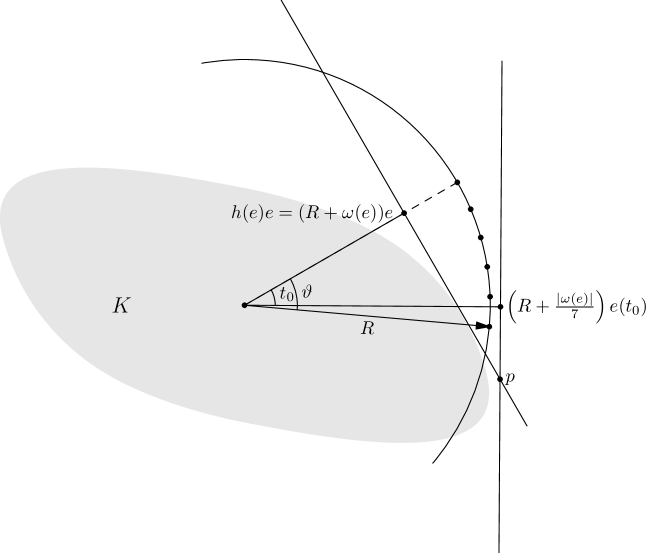
Figure 1. The body $K$, the lines $\langle x,e\rangle=R+\omega(e)$, $\langle x,e^{\prime}(t_{0})\rangle=R+\frac{1}{7}|\omega(e)|$, and the point $p$

Since $K$ is contained entirely in the angle $\langle x,e\rangle\leq R+\omega(e)$, $\langle x,e^{\prime}(t_{0})\rangle\leq R+\frac{1}{7}|\omega(e)|$ with vertex $p$, we have $h_{K}(e^{\prime}(t))\leq\langle p,e^{\prime}(t)\rangle=|p|\cos(\alpha-t)$ for all $t\in[0,t_{0}]$.

We shall now use the following elementary property of the cosine function: if $\gamma$, $\delta$$>0$ and $[\gamma-\delta,\gamma+\delta]\subset[0,\frac{\pi}{2}]$, then $\cos\beta\leq\frac{3\cos(\gamma-\delta)+\cos(\gamma+\delta)}{4}$ for all $\beta\in[\gamma,\gamma+\delta]$. Indeed, since $\cos\beta\leq\cos\gamma$, it suffices to show that

$$\cos\gamma\leq\frac{3\cos(\gamma-\delta)+\cos(\gamma+\delta)}{4}=\cos\gamma\cos\delta+\frac{1}{2}\sin\gamma\sin\delta.$$

Rewriting this as $\cos\gamma(1-\cos\delta)\leq\frac{1}{2}\sin\gamma\sin\delta$ and using the identity $1-\cos\delta$ $=\frac{1-\cos^{2}\delta}{1+\cos\delta}$ $=\frac{\sin^{2}\delta}{1+\cos\delta}$, we see that we need to prove that $\frac{\cos\gamma}{1+\cos\delta}\sin^{2}\delta\leq\frac{1}{2}\sin\gamma\sin\delta$. However, since $0\leq\delta\leq\gamma\leq\frac{\pi}{2}$, we have $\cos\gamma\leq\cos\delta\leq 1$ and $\sin\gamma\geq\sin\delta$, so the left hand side is at most $\frac{1}{2}\sin^{2}\delta$ and the right hand side is at least that.

Applying this property to the interval $[\alpha-t_{0},\alpha]$, i.e., with $\gamma=\alpha-\frac{t_{0}}{2}$, $\delta=\frac{t_{0}}{2}$, we conclude that

$$h_{K}(e^{\prime}(t))\leq\frac{3}{4}\Bigl{(}R+\frac{1}{7}|\omega(e)|\Bigr{)}+\frac{1}{4}(R+\omega(e))=R-\frac{1}{7}|\omega(e)|$$

for every $t\in[0,\frac{t_{0}}{2}]\supset[\frac{\vartheta}{5},\frac{2\vartheta}{5}]$ and the conclusion of the lemma follows again. ∎

Corollary 1.

Let $K$ be a convex body in ${\mathbb{R}^{n}}$ and let $R>0$. Let $h_{K}=R+\omega$ be the support function of $K$ and let $e\in S^{n-1}$ be a unit vector. Assume that $h_{K}(e)\leq R\cos\vartheta$ for some $\vartheta\in(0,\frac{\pi}{2})$. Then

$$|\omega(e)|\leq C\,\frac{1}{\sigma(S_{\vartheta}(e))}\int_{S_{\vartheta}(e)}|\omega(e^{\prime})|d\sigma(e^{\prime}).$$

Proof.

We will use the parametrization $e^{\prime}=e^{\prime}(t,v)\in S^{n-1}$ where $t$ is the angle between $e$ and $e^{\prime}$, and $v\in S^{n-1}\cap e^{\perp}$ is such that $e^{\prime}=e\cos t+v\sin t$.

Note that $d\sigma_{n-1}(e^{\prime})=c_{n}(\sin t)^{n-2}dtd\sigma_{n-2}(v)$. It follows from the lemma applied to the projection of $K$ to the plane spanned by $e$ and $v$ that

$$|\omega(e)|\leq\frac{35}{\vartheta}\int_{\frac{\vartheta}{5}}^{\vartheta}|\omega(e^{\prime}(t,v))|dt\leq\frac{35}{\vartheta\left(\sin(\frac{\vartheta}{5})\right)^{n-2}}\int_{0}^{\vartheta}|\omega(e^{\prime}(t,v))|(\sin t)^{n-2}dt.$$

Integrating this inequality with respect to $v$ and observing that $\sigma(S_{\vartheta}(e))\asymp\vartheta^{n-1}\asymp\vartheta(\sin(\frac{\vartheta}{5}))^{n-2}$, we get the statement of the corollary. ∎

Lemma 2.

Assume that a symmetric convex body $K$ is very close to the unit ball and $l\in{\mathbb{N}}$. Let $h=h_{K}$ and $\rho=\rho_{K}$ be the support and the radial functions of $K$ respectively. Trivially, $\rho\leq h$. Let $h=\sum\limits_{m=0}^{\infty}h_{m}$ be the decomposition of $h$ into spherical harmonics (since $h$ is even, only $h_{m}$ with even $m$ are not identically $0$). Put $\eta=\sum\limits_{m=1}^{l}h_{m}$, $\nu=\sum\limits_{m=l+1}^{\infty}h_{m}$. We claim that for every $\varepsilon,l>0$ there exists $\delta_{0}=\delta_{0}(\varepsilon,l)$ such that whenever $\|h-1\|_{\infty}\leq\delta_{0}$, the inequality

$$h-\rho\leq\varepsilon\|\eta\|_{L^{2}}+CM\nu$$

holds, where $C$ is an absolute constant and $M$ is the spherical Hardy-Littlewood maximal function.

Proof.

We have

$$\rho(e)=\inf\limits_{\{e^{\prime}\in S^{n-1},\langle e,e^{\prime}\rangle>0\}}\frac{h(e^{\prime})}{\langle e,e^{\prime}\rangle}.$$

Note that the admissible range of $e^{\prime}$ can be further restricted to $|e-e^{\prime}|<\delta$ with arbitrarily small $\delta>0$, provided that $\delta_{0}$ is chosen small enough. Indeed, since $h(e^{\prime})\geq\frac{1-\delta_{0}}{1+\delta_{0}}h(e)$, $e^{\prime}$ can compete with $e$ only if $\langle e,e^{\prime}\rangle\geq\frac{1-\delta_{0}}{1+\delta_{0}}$, so

$$|e-e^{\prime}|^{2}=2(1-\langle e,e^{\prime}\rangle)\leq\frac{4\delta_{0}}{1+\delta_{0}}<\delta^{2}$$

if $\delta_{0}>0$ is chosen appropriately. Now observe also that all norms on the finite-dimensional space of polynomials of degree not exceeding $l$ on the unit sphere are equivalent, and that any semi-norm is dominated by any norm, whence

$$\|\eta\|_{C(S^{n-1})}\leq C(l)\|\eta\|_{L^{2}(S^{n-1})}\qquad\textrm{and}\qquad\|\nabla\eta\|_{C(S^{n-1})}\leq C(l)\|\eta\|_{L^{2}(S^{n-1})}.$$

In particular, if $|e-e^{\prime\prime}|<2\delta$, we get

$$|\eta(e)-\eta(e^{\prime\prime})|\leq 4\|\nabla\eta\|_{C(S^{n-1})}\delta\leq 4C(l)\delta\|\eta\|_{L^{2}(S^{n-1})}.$$

Let us now assume that $e^{\prime}\in S^{n-1}$, with $|e-e^{\prime}|<\delta$, is a competitor, so $\frac{h(e^{\prime})}{\langle e,e^{\prime}\rangle}\leq h(e)$. Then, if $\vartheta$ is the angle between $e$ and $e^{\prime}$, we have $h(e^{\prime})\leq h(e)\cos\vartheta$, so we can apply Corollary 1 to the vector $e^{\prime}$ with $R=h(e)$ and conclude that

$$h(e)-\frac{h(e^{\prime})}{\langle e,e^{\prime}\rangle}\leq h(e)-h(e^{\prime})\leq\frac{C}{\sigma(S_{\vartheta}(e^{\prime}))}\int\limits_{S_{\vartheta}(e^{\prime})}|h(e)-h(e^{\prime\prime})|d\sigma(e^{\prime\prime})$$

$$\leq\frac{C^{\prime}}{\sigma(S_{2\vartheta}(e))}\int\limits_{S_{2\vartheta}(e)}|h(e)-h(e^{\prime\prime})|d\sigma(e^{\prime\prime}).$$

However,

$$|h(e)-h(e^{\prime\prime})|\leq|\eta(e)-\eta(e^{\prime\prime})|+|\nu(e)|+|\nu(e^{\prime\prime})|,$$

and

$$|\eta(e)-\eta(e^{\prime\prime})|\leq 4C(l)\delta\|\eta\|_{L^{2}(S^{n-1})},$$

while

$$|\nu(e)|\leq M\nu(e)\qquad\textrm{and}\qquad\frac{1}{\sigma(S_{2\vartheta}(e))}\int\limits_{S_{2\theta}(e)}|\nu(e^{\prime\prime})|d\sigma(e^{\prime\prime})\leq M\nu(e),$$

so the desired statement follows if we choose $\delta>0$ so that $4C^{\prime}C(l)\delta<\varepsilon$. ∎

7. Contraction

Let ${\mathfrak{M}}$ be a bounded linear operator on $L^{2}=L^{2}(S^{n-1})$ such that ${\mathfrak{M}}$ is proportional to the identity on every space ${\mathcal{H}}_{m}$ of spherical harmonics of degree $m$, i.e., for some $\mu_{m}\in{\mathbb{R}}$,

$${\mathfrak{M}}f=\sum\limits_{m\geq 0}\mu_{m}f_{m}\qquad\textrm{where}\qquad f=\sum\limits_{m\geq 0}f_{m}\qquad\textrm{and}\qquad f_{m}\in{\mathcal{H}}_{m}$$

is the spherical harmonic decomposition of $f\in L^{2}(S^{n-1})$. We say that ${\mathfrak{M}}$ is a strong contraction if

$$\max\limits_{m\geq 0}|\mu_{m}|<1,\quad\textrm{and}\qquad\lim\limits_{m\to\infty}\mu_{m}=0.$$

Lemma 3.

Assume that ${\mathfrak{M}}$ as above is a strong contraction. Then, there exists $\delta\in(0,1)$ such that for any symmetric convex body $K$ and any $c\in(1-\delta,1+\delta)$, the conditions

$$1-\delta\leq\rho_{K}\leq 1+\delta,\qquad\|(h_{K}-h_{\scriptscriptstyle{0}})-{c\,\mathfrak{M}}(\rho_{K}-r_{\scriptscriptstyle{0}})\|_{L^{2}}\leq\delta\|\rho_{K}-r_{\scriptscriptstyle{0}}\|_{L^{2}},$$

imply $h_{K}=\rho_{K}=const$. Here, $h_{\scriptscriptstyle{0}}$ and $r_{\scriptscriptstyle{0}}$ are the constant terms of the spherical harmonic decomposition of $h_{K}$ and $\rho_{K}$, respectively.

Proof.

Fix a large $l$ and consider the decompositions

$$h_{K}=h_{\scriptscriptstyle{0}}+\eta+\nu\qquad\textrm{and}\qquad\rho_{K}=r_{\scriptscriptstyle{0}}+\varphi+\psi,$$

where $h_{\scriptscriptstyle{0}}$, $r_{\scriptscriptstyle{0}}$ are the constant terms, $\eta$ and $\varphi$ are the parts corresponding to the harmonics of degrees $1$ to $l$ and $\nu$ and $\psi$ are the parts corresponding to the harmonics of degrees greater than $l$.

Fix $\varepsilon>0$. Since the projection to any sum of spaces of spherical harmonics in $L^{2}$ has norm $1$, we have

(8) $$\|\eta-c\,{\mathfrak{M}}\varphi\|_{L^{2}}\leq\|h_{K}-h_{\scriptscriptstyle{0}}-c\,{\mathfrak{M}}(\rho_{K}-r_{\scriptscriptstyle{0}})\|_{L^{2}}\leq$$

$$\delta\|\rho_{K}-r_{\scriptscriptstyle{0}}\|_{L^{2}}\leq\delta(\|\varphi\|_{L^{2}}+\|\psi\|_{L^{2}}).$$

Similarly,

(9) $$\|\nu-c\,{\mathfrak{M}}\psi\|_{L^{2}}\leq\delta(\|\varphi\|_{L^{2}}+\|\psi\|_{L^{2}}).$$

From (9) we obtain that

$$\|\nu\|_{L^{2}}\leq c\,\|{\mathfrak{M}}\psi\|_{L^{2}}+\delta(\|\varphi\|_{L^{2}}+\|\psi\|_{L^{2}})\leq$$

(10) $$(1+\delta)(\max\limits_{m>l}|\mu_{m}|)\|\psi\|_{L^{2}}+\delta(\|\varphi\|_{L^{2}}+\|\psi\|_{L^{2}})\leq\varepsilon(\|\varphi\|_{L^{2}}+\|\psi\|_{L^{2}})$$

if $l$ is large enough (recall that $\lim\limits_{m\to\infty}\mu_{m}=0$) and $\delta$ is small enough. The same computation for $\eta$, using in this case that $\max\limits_{m\geq 0}|\mu_{m}|<1$, yields

(11) $$\|\eta\|_{L^{2}}\leq(1+2\delta)(\|\varphi\|_{L^{2}}+\|\psi\|_{L^{2}}).$$

On the other hand, by Lemma 2 and the boundedness of the maximal function in $L^{2}$, we have

$$\|h_{K}-\rho_{K}\|_{L^{2}}\leq\varepsilon\|\eta\|_{L^{2}}+C\|\nu\|_{L^{2}},$$

which implies

(12) $$\|\eta-\varphi\|_{L^{2}}\leq\varepsilon\|\eta\|_{L^{2}}+C\|\nu\|_{L^{2}}\quad\textrm{and}\quad\|\nu-\psi\|_{L^{2}}\leq\varepsilon\|\eta\|_{L^{2}}+C\|\nu\|_{L^{2}}.$$

Combining (8), (9), (10), (11), and (12), we obtain

$$\|\varphi-c\,{\mathfrak{M}}\varphi\|_{L^{2}}+\|\psi-c\,{\mathfrak{M}}\psi\|_{L^{2}}$$

$$\leq\|\varphi-\eta\|_{L^{2}}+\|\eta-c\,{\mathfrak{M}}\varphi\|_{L^{2}}+\|\psi-\nu\|_{L^{2}}+\|\nu-c\,{\mathfrak{M}}\psi\|_{L^{2}}$$

$$\leq C(\delta+\varepsilon)(\|\varphi\|_{L^{2}}+\|\psi\|_{L^{2}}).$$

On the other hand, for any function $\chi\in L^{2}(S^{n-1})$, we have

$$\|\chi-c\,{\mathfrak{M}}\chi\|_{L^{2}}\geq(1-(1+\delta)\max\limits_{m\geq 0}|\mu_{m}|)\|\chi\|_{L^{2}},$$

so we can conclude that $\varphi=0$, $\psi=0$ if $\,C(\delta+\varepsilon)<1-(1+\delta)\max\limits_{m\geq 0}|\mu_{m}|$. ∎

Remark 1.

Note that $(h_{K}-h_{\scriptscriptstyle{0}})-{c\,\mathfrak{M}}(\rho_{K}-r_{\scriptscriptstyle{0}})$ is orthogonal to constants and, therefore, its $L^{2}$-norm does not exceed $\|(h_{K}-\lambda)-{c\,\mathfrak{M}}(\rho_{K}-r_{\scriptscriptstyle{0}})\|_{L^{2}}$ for any $\lambda\in{\mathbb{R}}$. Thus, to verify the conditions of the lemma it suffices to check that

$$\|(h_{K}-\lambda)-{c\,\mathfrak{M}}(\rho_{K}-r_{\scriptscriptstyle{0}})\|_{L^{2}}\leq\delta\|\rho_{K}-r_{\scriptscriptstyle{0}}\|_{L^{2}}$$

with any $\lambda\in{\mathbb{R}}$ of our choice.

8. Properties of the function $(\mathcal{R}[\rho_{K}^{\alpha}])^{\beta}$ when $\rho_{K}$ is close to $1$

Let $K$ be a symmetric convex body in the isotropic position such that $1-\delta\leq\rho_{K}\leq 1+\delta$ for some small $\delta>0$. Let $\alpha,\beta\in{\mathbb{R}}$. We want to derive several useful properties of the function $(\mathcal{R}[\rho_{K}^{\alpha}])^{\beta}$.

The first observation is that $\rho_{K}$ is Lipschitz with Lipschitz constant $5\sqrt{\delta}$. Indeed, let $x,y\in S^{n-1}$. If $|x-y|\geq\frac{\sqrt{\delta}}{2}$, then we have

$$|\rho_{K}(x)-\rho_{K}(y)|\leq 2\delta\leq 4\sqrt{\delta}|x-y|,$$

so we may assume that $0<|x-y|<\frac{\sqrt{\delta}}{2}$. Without loss of generality, $\rho_{K}(x)\geq\rho_{K}(y)$. Let us denote $X=\rho_{K}(x)x$, $Y=\rho_{K}(y)y$, where $X,Y\in\partial K$. By the convexity of $K$, every point on the line $Y-t(X-Y)$ with $t\geq 0$ lies outside $K$ and, therefore, outside $(1-\delta)B_{2}^{n}$ as well. Hence,

$$(1-\delta)^{2}\leq|Y-t(X-Y)|^{2}=|Y|^{2}-2t\langle X-Y,Y\rangle+t^{2}|X-Y|^{2}.$$

Since $|Y|^{2}\leq(1+\delta)^{2}$, we conclude that, for all $t\geq 0$,

(13) $$2t\langle X-Y,Y\rangle-t^{2}|X-Y|^{2}\leq 4\delta.$$

From (13) it follows that

(14) $$\langle X-Y,Y\rangle\leq 2\sqrt{\delta}|X-Y|.$$

Indeed, if $\langle X-Y,Y\rangle\leq 0$, the inequality is obvious. Otherwise, we can plug $t=\frac{\langle X-Y,Y\rangle}{|X-Y|^{2}}$ into (13), obtaining $\frac{\langle X-Y,Y\rangle^{2}}{|X-Y|^{2}}\leq 4\delta$, which is equivalent to (14). Now, equation (14) can be rewritten as

$$|X||Y|\langle x,y\rangle-|Y|^{2}\leq 2\sqrt{\delta}|X-Y|,$$

or, equivalently,

$$|Y|\left(|X|-|Y|\right)\leq 2\sqrt{\delta}|X-Y|+|X||Y|(1-\langle x,y\rangle).$$

Observe that $1-\langle x,y\rangle=\frac{1}{2}|x-y|^{2}\leq\frac{\sqrt{\delta}}{4}|x-y|$, while $|X-Y|\leq|X|-|Y|+|Y||x-y|$. Hence,

$$|X|-|Y|\leq\frac{2\sqrt{\delta}}{|Y|}\left(|X|-|Y|\right)+\left(2+\frac{|X|}{4}\right)\sqrt{\delta}|x-y|.$$

Now, if $\delta\in(0,1/25)$,

$$\frac{2\sqrt{\delta}}{|Y|}\leq\frac{2\sqrt{\delta}}{1-\delta}\leq\frac{2/5}{1-1/25}<\frac{1}{2},$$

and we conclude that

$$|X|-|Y|\leq 2\left(2+\frac{|X|}{4}\right)\sqrt{\delta}|x-y|\leq\left(4+\frac{1+\delta}{2}\right)\sqrt{\delta}|x-y|\leq 5\sqrt{\delta}|x-y|,$$

as required.

Since the mapping $t\mapsto t^{p}$ is Lipschitz on any compact subset of $(0,+\infty)$ and the Radon transform does not increase the Lipschitz constant of the function, we immediately conclude that $(\mathcal{R}[\rho_{K}^{\alpha}])^{\beta}$ has Lipschitz constant at most $C_{\alpha,\beta}\sqrt{\delta}$.

Let now $r_{\scriptscriptstyle{0}}=\int\limits_{S^{n-1}}\rho_{K}d\sigma$ be the mean value of $\rho_{K}$ on the unit sphere. Clearly, $|r_{\scriptscriptstyle{0}}-1|\leq\delta$, so $|\rho_{K}-r_{\scriptscriptstyle{0}}|\leq 2\delta$ and, thereby, $\mathcal{R}|\rho_{K}-r_{\scriptscriptstyle{0}}|\leq 2\delta$ as well. Now, using the fact that $t\mapsto t^{p}$ is $C^{2}$ on any compact subset of $(0,+\infty)$ and linearizing, we successively derive that

$$|\rho_{K}^{\alpha}-(r_{\scriptscriptstyle{0}}^{\alpha}+\alpha r_{\scriptscriptstyle{0}}^{\alpha-1}(\rho_{K}-r_{\scriptscriptstyle{0}}))|\leq C_{\alpha}\delta|\rho_{K}-r_{\scriptscriptstyle{0}}|,$$

$$|\mathcal{R}[\rho_{K}^{\alpha}]-(r_{\scriptscriptstyle{0}}^{\alpha}+\alpha r_{\scriptscriptstyle{0}}^{\alpha-1}\mathcal{R}(\rho_{K}-r_{\scriptscriptstyle{0}}))|\leq C_{\alpha}\,\delta\mathcal{R}|\rho_{K}-r_{\scriptscriptstyle{0}}|,$$

$$|(\mathcal{R}[\rho_{K}^{\alpha}])^{\beta}-(r_{\scriptscriptstyle{0}}^{\alpha}+\alpha r_{\scriptscriptstyle{0}}^{\alpha-1}\mathcal{R}(\rho_{K}-r_{\scriptscriptstyle{0}}))^{\beta}|\leq C_{\alpha,\beta}\,\delta\mathcal{R}|\rho_{K}-r_{\scriptscriptstyle{0}}|,$$

$$|(\mathcal{R}[\rho_{K}^{\alpha}])^{\beta}-(r_{\scriptscriptstyle{0}}^{\alpha\beta}+\alpha\beta r_{\scriptscriptstyle{0}}^{\alpha\beta-1}\mathcal{R}(\rho_{K}-r_{\scriptscriptstyle{0}}))|\leq C_{\alpha,\beta}\,\delta\mathcal{R}|\rho_{K}-r_{\scriptscriptstyle{0}}|.$$

Thus, $(\mathcal{R}[\rho_{K}^{\alpha}])^{\beta}=r_{\scriptscriptstyle{0}}^{\alpha\beta}+\gamma$, where

$$|\gamma-\alpha\beta r_{\scriptscriptstyle{0}}^{\alpha\beta-1}\mathcal{R}(\rho_{K}-r_{\scriptscriptstyle{0}})|\leq C_{\alpha,\beta}\,\delta\mathcal{R}|\rho_{K}-r_{\scriptscriptstyle{0}}|.$$

In particular, we conclude that $|\gamma|\leq C_{\alpha,\beta}\,\delta$, which, together with the above observation about the Lipschitz constant, implies that

$$\|\gamma\|_{C^{\frac{1}{2}}}=\max\limits_{S^{n-1}}|\gamma|+\sup\limits_{x,y\in S^{n-1},x\neq y}\,\frac{|\gamma(x)-\gamma(y)|}{|x-y|^{\frac{1}{2}}}\leq C_{\alpha,\beta}\,\sqrt{\delta}.$$

Now let $\rho_{K}-r_{\scriptscriptstyle{0}}=Y_{2}+Y_{4}+\dots$ be the spherical harmonic decomposition of $\rho_{K}-r_{\scriptscriptstyle{0}}$. It follows from the definition of the isotropic position that

$$0=\int\limits_{K}p(x)dx=c_{n}\int\limits_{S^{n-1}}\rho_{K}^{n+2}(x)p(x)d\sigma(x)$$

for all quadratic polynomials $p(x)=\sum\limits_{i,j}a_{ij}x_{i}x_{j}$ with $\sum\limits_{i=1}^{n}a_{ii}=0$. In other words, $\rho_{K}^{n+2}$ has no second order term in its spherical harmonic decomposition.

On the other hand,

$$|\rho_{K}^{n+2}-(r_{\scriptscriptstyle{0}}^{n+2}+(n+2)r_{\scriptscriptstyle{0}}^{n+1}(\rho_{K}-r_{\scriptscriptstyle{0}}))|\leq C\delta|\rho_{K}-r_{\scriptscriptstyle{0}}|.$$

Taking the second order component in the spherical harmonic decomposition of the expression under the absolute value sign on the left hand side, we get

$$(n+2)r_{\scriptscriptstyle{0}}^{n+1}\|Y_{2}\|_{L^{2}(S^{n-1})}\leq C\delta\|\rho_{K}-r_{\scriptscriptstyle{0}}\|_{L^{2}(S^{n-1})},$$

so

$$\|Y_{2}\|_{L^{2}(S^{n-1})}\leq C^{\prime}\delta\|\rho_{K}-r_{\scriptscriptstyle{0}}\|_{L^{2}(S^{n-1})}.$$

9. A solution to the fifth Busemann-Petty problem in a small neighborhood of the Euclidean ball

Recall that for the fifth Busemann-Petty problem we have the equation $h_{K}=(\mathcal{R}[\rho_{K}^{n-1}])^{-1}$. By the results of the previous section, the right hand side can be written as

$$r_{\scriptscriptstyle{0}}^{-n+1}-(n-1)r_{\scriptscriptstyle{0}}^{-n}\mathcal{R}(\rho_{K}-r_{\scriptscriptstyle{0}})+\gamma^{\prime},$$

where $|\gamma^{\prime}|\leq C\delta\mathcal{R}|\rho_{K}-r_{\scriptscriptstyle{0}}|$, so $\|\gamma^{\prime}\|_{L^{2}(S^{n-1})}\leq C\delta\|\rho_{K}-r_{\scriptscriptstyle{0}}\|_{L^{2}(S^{n-1})}$.

Let ${\mathfrak{M}}$ be the linear operator that maps every $m$-th order spherical harmonic $Z_{m}$ to

$$-(n-1)\mathcal{R}Z_{m}=-(n-1)(-1)^{\frac{m}{2}}\frac{1\cdot 3\cdot\ldots\cdot(m-1)}{(n-1)(n+1)\cdot\ldots\cdot(n+m-3)}Z_{m}$$

for even $m\geq 4$ and to $0$ for other $m$. Then ${\mathfrak{M}}$ is a strong contraction and

$$\|(h_{K}-r_{\scriptscriptstyle{0}}^{-n+1})-r_{\scriptscriptstyle{0}}^{-n}{\mathfrak{M}}(\rho_{K}-r_{\scriptscriptstyle{0}})\|_{L^{2}(S^{n-1})}\leq$$

$$r_{\scriptscriptstyle{0}}^{-n}\|Y_{2}\|_{L^{2}(S^{n-1})}+\|\gamma^{\prime}\|_{L^{2}(S^{n-1})}\leq C\delta\|\rho_{K}-r_{\scriptscriptstyle{0}}\|_{L^{2}(S^{n-1})},$$

so Lemma 3 and Remark 1 yield $h_{K}=\rho_{K}=const$, i.e., $K$ is a ball, provided that $\delta$ is small enough.

10. A solution to the eighth Busemann-Petty problem in a small neighborhood of the Euclidean ball

We now turn to the equation $Ah_{K}=(\mathcal{R}[\rho_{K}^{n-1}])^{n+1}$ (see Section 5). Below we will use several standard results about $A$ and the Laplace operator which, for completeness, are proven in the Appendices.

By the results of Section 8, $(\mathcal{R}[\rho_{K}^{n-1}])^{n+1}$ can be rewritten as $r_{\scriptscriptstyle{0}}^{(n-1)(n+1)}+\gamma$, where $\|\gamma\|_{C^{\frac{1}{2}}}\leq C\sqrt{\delta}$ and

$$\gamma=(n-1)(n+1)r_{\scriptscriptstyle{0}}^{(n-1)(n+1)-1}\mathcal{R}(\rho_{K}-r_{\scriptscriptstyle{0}})+\gamma^{\prime},$$

$$\|\gamma^{\prime}\|_{L^{2}(S^{n-1})}\leq C\delta\|\rho_{K}-r_{\scriptscriptstyle{0}}\|_{L^{2}(S^{n-1})}.$$

Then

$$A\frac{h_{K}}{r_{\scriptscriptstyle{0}}^{n+1}}=1+r_{\scriptscriptstyle{0}}^{-(n-1)(n+1)}\gamma$$

and, provided that $\delta>0$ is small enough, we can apply Lemma 4 (see Appendix II) and the uniqueness theorem (see [Sch], Theorem 8.1.1) to obtain

$$\frac{h_{K}}{r_{\scriptscriptstyle{0}}^{n+1}}=1+\varphi^{\prime}+\varphi^{\prime\prime},$$

where

(15) $$\widetilde{\Delta}\varphi^{\prime}=r_{\scriptscriptstyle{0}}^{-(n-1)(n+1)}\gamma$$

(see Appendix II for the definition of $\widetilde{\Delta}$) and

$$\|\varphi^{\prime\prime}\|_{L^{2}(S^{n-1})}\leq\varepsilon r_{\scriptscriptstyle{0}}^{-(n-1)(n+1)}\|\gamma\|_{L^{2}(S^{n-1})}\leq C\varepsilon\|\rho_{K}-r_{\scriptscriptstyle{0}}\|_{L^{2}(S^{n-1})}$$

with as small $\varepsilon>0$ as we want.

Furthermore, the solution of equation (15) splits into $\varphi^{\prime}_{1}+\varphi_{2}^{\prime}$ where $\varphi_{1}^{\prime}$ solves

$$\widetilde{\Delta}\varphi_{1}^{\prime}=(n-1)(n+1)r_{\scriptscriptstyle{0}}^{-1}{\mathcal{R}}(\rho_{K}-r_{\scriptscriptstyle{0}}),$$

and $\varphi_{2}^{\prime}$ solves $\widetilde{\Delta}\varphi_{2}^{\prime}=r_{\scriptscriptstyle{0}}^{-(n-1)(n+1)}\gamma^{\prime}$.

The norm of $\varphi_{2}^{\prime}$ can be estimated immediately:

$$\|\varphi_{2}^{\prime}\|_{L^{2}(S^{n-1})}\leq C\|\gamma^{\prime}\|_{L^{2}(S^{n-1})}\leq C\delta\|\rho_{K}-r_{\scriptscriptstyle{0}}\|_{L^{2}(S^{n-1})}.$$

As to $\varphi_{1}^{\prime}$, it is equal to (see the end of Appendix I)

$$r_{\scriptscriptstyle{0}}^{-1}\sum\limits_{{\begin{subarray}{c}m\geq 2\\ m\,\text{even}\end{subarray}}}\mu_{m}Y_{m},$$

where $\rho_{K}=r_{\scriptscriptstyle{0}}+\sum\limits_{{\begin{subarray}{c}m\geq 2\\ m\,\text{even}\end{subarray}}}Y_{m}\,$ is the spherical harmonic decomposition of $\rho_{K}$ and

$$\mu_{m}=\frac{(n-1)(n+1)}{(1-m)(m+n-1)}(-1)^{\frac{m}{2}}\frac{1\cdot 3\cdot\ldots\cdot(m-1)}{(n-1)(n+1)\cdot\ldots\cdot(n+m-3)},$$

so $\mu_{2}=1$ and $|\mu_{m}|<1$ for $m\geq 4$, $\mu_{m}\to 0$ as $m\to\infty$. Since

$$\|Y_{2}\|_{L^{2}(S^{n-1})}\leq C\delta\|\rho_{K}-r_{\scriptscriptstyle{0}}\|_{L^{2}(S^{n-1})},$$

we conclude that

$$\|\varphi_{1}^{\prime}-r_{\scriptscriptstyle{0}}^{-1}{\mathfrak{M}}(\rho_{K}-r_{\scriptscriptstyle{0}})\|_{L^{2}(S^{n-1})}\leq C\delta\|\rho_{K}-r_{\scriptscriptstyle{0}}\|_{L^{2}(S^{n-1})},$$

with the strong contraction ${\mathfrak{M}}$ given by $Z_{m}\mapsto\mu_{m}Z_{m}$, $m$ even, $m\geq 4$; $Z_{m}\mapsto 0$ for all other $m$.

Putting all these estimates together, we conclude that

$$\|(h_{K}-r_{\scriptscriptstyle{0}}^{n+1})-r_{\scriptscriptstyle{0}}^{n}{\mathfrak{M}}(\rho_{K}-r_{\scriptscriptstyle{0}})\|_{L^{2}(S^{n-1})}\leq\varepsilon\|\rho_{K}-r_{\scriptscriptstyle{0}}\|_{L^{2}(S^{n-1})},$$

with as small $\varepsilon>0$ as we want, provided that $\delta>0$ is small enough. Now we can apply Lemma 3 and Remark 1 again to conclude that $h_{K}=\rho_{K}=const$, so $K$ is a ball.

11. Appendix I. Solving the Laplace equation

Below we shall use the following notation. For a function $f:S^{n-1}\to{\mathbb{R}}$ and $\alpha\in(0,1)$, we shall denote

$$\|f\|_{C^{\alpha}}=\|f\|_{C^{\alpha}(S^{n-1})}=\max\limits_{S^{n-1}}|f|+\sup\limits_{x,y\in S^{n-1},\,x\neq y}\frac{|f(x)-f(y)|}{|x-y|^{\alpha}},$$

$$\|f\|_{C^{2+\alpha}}=\|f\|_{C^{2+\alpha}(S^{n-1})}=$$

$$\max\limits_{S^{n-1}}|f|+\max\limits_{x\in S^{n-1},\,i=1,\dots,n}|F_{x_{i}}(x)|+\max\limits_{i,j=1,\dots,n}\|F_{x_{i}x_{j}}\|_{C^{\alpha}(S^{n-1})},$$

where $F(x)=|x|f(\frac{x}{|x|})$ is the $1$-homogeneous extension of $f$ to ${\mathbb{R}^{n}}\setminus\{0\}$ (we assume that it is at least $C^{2}$ in ${\mathbb{R}^{n}}\setminus\{0\}$).

Let $g:S^{n-1}\to{\mathbb{R}}$ be an even $C^{\alpha}$ function on the unit sphere $S^{n-1}$ with some $\alpha\in(0,1)$. Let ${\mathcal{G}}$ be the $(-1)$-homogeneous extension of $g$ to ${\mathbb{R}^{n}}\setminus\{0\}$, i.e., ${\mathcal{G}}(x)=|x|^{-1}g(\frac{x}{|x|})$ for $x\neq 0$. We will show that there exists a unique $1$-homogeneous even function $F:{\mathbb{R}^{n}}\to{\mathbb{R}}$ of class $L^{1}_{loc}$ such that $\Delta F={\mathcal{G}}$ in ${\mathbb{R}^{n}}$ in the sense of generalized functions. Moreover, $F\in C^{2+\alpha}(S^{n-1})$ and for all $i,j=1,\dots,n$, we have

(16) $$\|F_{x_{i}x_{j}}\|_{L^{2}(S^{n-1})}\leq C\|g\|_{L^{2}(S^{n-1})},\qquad\|F\|_{C^{2+\alpha}(S^{n-1})}\leq C\|g\|_{C^{\alpha}(S^{n-1})},$$

with some $C=C(n,\alpha)>0$.

11.1. Uniqueness

If we have two even $1$-homogeneous functions $F_{1}$, $F_{2}$ such that $\Delta F_{1}=\Delta F_{2}={\mathcal{G}}$ in ${\mathbb{R}^{n}}$, then $F_{1}-F_{2}$ is an even $1$-homogeneous harmonic function, but the only such function is $0$.

11.2. Existence

Now we will show that the function $F$ defined by

$$F(x)=c_{n}\int\limits_{\mathbb{R}^{n}}\Big{[}\frac{1}{|x-y|^{n-2}}-\frac{1}{|y|^{n-2}}\Big{]}{\mathcal{G}}(y)dy$$

is a well-defined $1$-homogeneous function on ${\mathbb{R}^{n}}$ satisfying $\Delta F={\mathcal{G}}$ and estimates (16). Here, $c_{n}$ is chosen so that $\Delta\frac{c_{n}}{|x|^{n-2}}=\delta_{0}$ (the Dirac delta measure) in the sense of generalized functions, and the integral is understood as $\lim\limits_{R\to\infty}\int\limits_{B(0,R)}$.

In order to show the convergence of the integral, we note that

$$\frac{1}{|x-y|^{n-2}}-\frac{1}{|y|^{n-2}}=(n-2)\frac{\langle x,y\rangle}{|y|^{n}}+O\Big{(}\frac{1}{|y|^{n}}\Big{)}$$

as $y\to\infty$ uniformly on compact sets in $x$.

Since ${\mathcal{G}}$ is even, the integral of $\frac{\langle x,y\rangle}{|y|^{n}}{\mathcal{G}}(y)$ over each sphere centered at the origin vanishes. Since ${\mathcal{G}}$ is $(-1)$-homogeneous, we have $\frac{1}{|y|^{n}}{\mathcal{G}}(y)=O(\frac{\|g\|_{C}}{|y|^{n+1}})$ as $y\to\infty$, which is integrable at $\infty$.

The singularities at $x\in S^{n-1}$ and $0$ are of degrees $-(n-2)$ and $-(n-1)$ respectively, so the local integrability there presents no problem either, and we get the estimate

$$\|F\|_{C(S^{n-1})}\leq C\|g\|_{C(S^{n-1})}.$$

The change of variable $y\mapsto-y$ and the identity ${\mathcal{G}}(y)={\mathcal{G}}(-y)$ imply that $F$ is even.

To show the $1$-homogeneity of $F$, take $t>0$ and apply the change of variable $y\mapsto ty$ to write

$$F(tx)=c_{n}\lim\limits_{R\to\infty}\int\limits_{B(0,R)}\Big{(}\frac{1}{|tx-y|^{n-2}}-\frac{1}{|y|^{n-2}}\Big{)}{\mathcal{G}}(y)dy=$$

$$c_{n}\lim\limits_{R\to\infty}\int\limits_{B(0,\frac{R}{t})}\Big{(}\frac{1}{|tx-ty|^{n-2}}-\frac{1}{|ty|^{n-2}}\Big{)}{\mathcal{G}}(ty)d(ty)=$$

$$c_{n}\,t\,\lim\limits_{R\to\infty}\int\limits_{B(0,\frac{R}{t})}\Big{(}\frac{1}{|x-y|^{n-2}}-\frac{1}{|y|^{n-2}}\Big{)}{\mathcal{G}}(y)dy=tF(x),$$

(we used that $\frac{1}{|tz|^{n-2}}=\frac{1}{t^{n-2}}\frac{1}{|z|^{n-2}}$, ${\mathcal{G}}(ty)=t^{-1}{\mathcal{G}}(y)$, and $d(ty)=t^{n}dy$).

To estimate $\|F\|_{C^{2+\alpha}(S^{n-1})}$, we split the integral defining $F$ into 3 parts. Let $\xi_{1}$, $\xi_{2}$, $\xi_{3}:[0,+\infty)$ $\to[0,1]$ be as on Figure 2, so $\xi_{i}$ are Lipschitz with constant 4, and $\xi_{1}+\xi_{2}+\xi_{3}=1$.

Figure 2. The functions $\xi_{i}$, $i=1,2,3$

Put ${\mathcal{G}}_{i}(x)={\mathcal{G}}(x)\xi_{i}(|x|)$ and

$$F_{i}(x)=c_{n}\int\limits_{{\mathbb{R}^{n}}}\Big{[}\frac{1}{|x-y|^{n-2}}-\frac{1}{|y|^{n-2}}\Big{]}{\mathcal{G}}_{i}(y)dy,$$

so ${\mathcal{G}}={\mathcal{G}}_{1}+{\mathcal{G}}_{2}+{\mathcal{G}}_{3}$ and $F=F_{1}+F_{2}+F_{3}$.

Our first observation is that ${\mathcal{G}}_{2}(y)$ is an $\alpha$-Hölder, compactly supported function on ${\mathbb{R}^{n}}$, with $C^{\alpha}$-norm bounded by $C\|g\|_{C^{\alpha}(S^{n-1})}$.

Indeed, we clearly have $\max\limits_{\mathbb{R}^{n}}|{\mathcal{G}}_{2}|\leq 4\max\limits_{S^{n-1}}|g|$. On the other hand,

$$|{\mathcal{G}}_{2}(x)-{\mathcal{G}}_{2}(y)|=\Big{|}\xi_{2}(|x|)|x|^{-1}g\Big{(}\frac{x}{|x|}\Big{)}-\xi_{2}(|y|)|y|^{-1}g\Big{(}\frac{y}{|y|}\Big{)}\Big{|}.$$

Since $\widetilde{\xi}_{2}(t)=\xi_{2}(t)t^{-1}$ is a compactly supported Lipschitz function on $[0,+\infty)$, it is also $\alpha$-Hölder for any $\alpha\in(0,1)$, i.e.,

$$|\widetilde{\xi}_{2}(t)-\widetilde{\xi}_{2}(s)|\leq C|t-s|^{\alpha}\quad\textrm{for all}\quad t,s\geq 0.$$

Thus, if $x,y\in\overline{B(0,2)}\setminus B(0,\frac{1}{4})$, then

$$\left|\widetilde{\xi}_{2}(|x|)g\left(\frac{x}{|x|}\right)-\widetilde{\xi}_{2}(|y|)g\left(\frac{y}{|y|}\right)\right|\leq$$

$$|\widetilde{\xi}_{2}(|x|)-\widetilde{\xi}_{2}(|y|)|\,\left|g\left(\frac{x}{|x|}\right)\right|+|\widetilde{\xi}_{2}(|y|)|\,\left|g\left(\frac{x}{|x|}\right)-g\left(\frac{y}{|y|}\right)\right|\leq$$

$$C\,\Bigl{|}|x|-|y|\Bigr{|}^{\alpha}\max\limits_{S^{n-1}}|g|+4\Big{|}\frac{x}{|x|}-\frac{y}{|y|}\Big{|}^{\alpha}\|g\|_{C^{\alpha}(S^{n-1})}\leq$$

$$C\,\|g\|_{C^{\alpha}(S^{n-1})}\Big{(}|x-y|^{\alpha}+\Big{|}\frac{x}{|x|}-\frac{y}{|y|}\Big{|}^{\alpha}\Big{)}\leq C\,\|g\|_{C^{\alpha}(S^{n-1})}|x-y|^{\alpha},$$

because the mapping $x\mapsto\frac{x}{|x|}$ is $C^{1}$ and, thereby, Lipschitz on $\overline{B(0,2)}\setminus B(0,\frac{1}{4})$.

If $x,y\notin\overline{B(0,2)}\setminus B(0,\frac{1}{4})$, then ${\mathcal{G}}_{2}(x)={\mathcal{G}}_{2}(y)=0$, so the inequality

$$|{\mathcal{G}}_{2}(x)-{\mathcal{G}}_{2}(y)|\leq C\,\|g\|_{C^{\alpha}(S^{n-1})}|x-y|^{\alpha}$$

holds trivially. Finally, if $x\in\overline{B(0,2)}\setminus B(0,\frac{1}{4})$ but $y\notin\overline{B(0,2)}\setminus B(0,\frac{1}{4})$, then the segment $[x,y]$ intersects the boundary of $\overline{B(0,2)}\setminus B(0,\frac{1}{4})$ at some point $y^{\prime}$, so ${\mathcal{G}}_{2}(y)={\mathcal{G}}_{2}(y^{\prime})=0$ and

$$|{\mathcal{G}}_{2}(x)-{\mathcal{G}}_{2}(y)|=|{\mathcal{G}}_{2}(x)-{\mathcal{G}}_{2}(y^{\prime})|\leq$$

$$C\,\|g\|_{C^{\alpha}(S^{n-1})}|x-y^{\prime}|^{\alpha}\leq C\,\|g\|_{C^{\alpha}(S^{n-1})}|x-y|^{\alpha}.$$

The functions ${\mathcal{G}}_{1}$ and ${\mathcal{G}}_{3}$ are supported on $\overline{B(0,\frac{1}{2})}$ and ${\mathbb{R}^{n}}\setminus B(0,\frac{3}{2})$, respectively, and satisfy the bound

$$|{\mathcal{G}}_{1}(y)|,\,|{\mathcal{G}}_{3}(y)|\leq\frac{1}{|y|}\max\limits_{S^{n-1}}|g|.$$

Now we are ready to estimate $\|F\|_{C^{2+\alpha}(S^{n-1})}$. Consider $x$ with $\frac{3}{4}\leq|x|\leq\frac{5}{4}$. Note that $x\mapsto\frac{1}{|x-y|^{n-2}}$ is a $C^{3}$-function (in $x$) in this domain with uniformly bounded (in $y$) $C^{3}$-norm as long as $y\in\overline{B(0,\frac{1}{2})}$. Hence, $F_{1}\in C^{3}(\overline{B(0,\frac{5}{4})}\setminus B(0,\frac{3}{4}))$ and

$$\|F_{1}\|_{C^{3}(\overline{B(0,\frac{5}{4})}\setminus B(0,\frac{3}{4}))}\leq C\|g\|_{L^{1}(S^{n-1})}$$

(the constant term $\int\limits_{{\mathbb{R}^{n}}}\frac{1}{|y|^{n-2}}{\mathcal{G}}_{1}(y)dy$ is also bounded by $C\|g\|_{L^{1}(S^{n-1})}$).

To estimate $F_{3}$, note that for $|x|\leq\frac{5}{4}$ and $|y|\geq\frac{3}{2}$, we have

$$\Big{|}\frac{1}{|x-y|^{n-2}}-\frac{1}{|y|^{n-2}}-(n-2)\frac{\langle x,y\rangle}{|y|^{n}}\Big{|}\leq\frac{C}{|y|^{n}},$$

$$\Big{|}\frac{\partial}{\partial x_{i}}\frac{1}{|x-y|^{n-2}}-(n-2)\frac{y_{i}}{|y|^{n}}\Big{|}\leq\frac{C}{|y|^{n}},$$

$$\Big{|}\frac{\partial^{2}}{\partial x_{i}\partial x_{j}}\frac{1}{|x-y|^{n-2}}\Big{|}\leq\frac{C}{|y|^{n}},$$

and

$$\Big{|}\frac{\partial^{3}}{\partial x_{i}\partial x_{j}\partial x_{k}}\frac{1}{|x-y|^{n-2}}\Big{|}\leq\frac{C}{|y|^{n+1}}.$$

Since $y\mapsto\frac{\langle x,y\rangle}{|y|^{n}}$ and $y\mapsto\frac{y_{i}}{|y|^{n}}$ are odd functions, their integrals against the even function ${\mathcal{G}}_{3}(y)$ over any sphere centered at the origin are $0$ and, therefore,

$$|F_{3}|,|\nabla F_{3}|,|\nabla^{2}F_{3}|\leq C\int\limits_{{\mathbb{R}^{n}}\setminus B(0,\frac{3}{2})}|y|^{-n}|{\mathcal{G}}_{3}(y)|dy\leq C\|g\|_{L^{1}(S^{n-1})}$$

and

$$|\nabla^{3}F_{3}|\leq C\int\limits_{{\mathbb{R}^{n}}\setminus B(0,\frac{3}{2})}|y|^{-n-1}|{\mathcal{G}}_{3}(y)|dy\leq C\|g\|_{L^{1}(S^{n-1})},$$

so

$$\|F_{3}\|_{C^{3}(\overline{B(0,\frac{5}{4})})}\leq C\|g\|_{L^{1}(S^{n-1})}.$$

It remains to estimate $F_{2}$. We clearly have

$$|F_{2}(x)|\leq C\|g\|_{C(S^{n-1})}\int\limits_{\overline{B(0,2)}\setminus B(0,\frac{1}{4})}\Big{|}\frac{1}{|x-y|^{n-2}}-\frac{1}{|y|^{n-2}}\Big{|}dy\leq C\|g\|_{C(S^{n-1})}$$

and

$$|\nabla F_{2}(x)|\leq C\|g\|_{C(S^{n-1})}\int\limits_{\overline{B(0,2)}\setminus B(0,\frac{1}{4})}\frac{1}{|x-y|^{n-1}}dy\leq C\|g\|_{C(S^{n-1})}.$$

As for $(F_{2})_{x_{i}x_{j}}$, these partial derivatives are images of ${\mathcal{G}}_{2}$ under certain Calderón-Zygmund singular integral operators (see [GT], Lemma 4.4 and Theorem 9.9), so, since ${\mathcal{G}}_{2}\in C^{\alpha}{({\mathbb{R}^{n}})}$ and has fixed compact support, we obtain that

$$\|(F_{2})_{x_{i}x_{j}}\|_{C^{\alpha}({\mathbb{R}^{n}})}\leq C\|{\mathcal{G}}_{2}\|_{C^{\alpha}({\mathbb{R}^{n}})}\leq C\|g\|_{C^{\alpha}(S^{n-1})}$$

and

$$\|(F_{2})_{x_{i}x_{j}}\|_{L^{2}({\mathbb{R}^{n}})}\leq C\|{\mathcal{G}}_{2}\|_{L^{2}({\mathbb{R}^{n}})}\leq C\|g\|_{L^{2}(S^{n-1})}.$$

The final conclusion is that

$$\|F\|_{C^{2+\alpha}(S^{n-1})}\leq C\|F\|_{C^{2+\alpha}(\overline{B(0,\frac{5}{4})}\setminus B(0,\frac{3}{4}))}\leq C\|g\|_{C^{\alpha}(S^{n-1})}$$

and

$$\|(F_{2})_{x_{i}x_{j}}\|_{L^{2}(S^{n-1})}\leq C\|(F_{2})_{x_{i}x_{j}}\|_{L^{2}(\overline{B(0,\frac{5}{4})}\setminus B(0,\frac{3}{4}))}\leq C\|g\|_{L^{2}(S^{n-1})}$$

(we used the $(-1)$-homogeneity of $(F_{2})_{x_{i}x_{j}}$ here).

The desired equality $\Delta F={\mathcal{G}}$ follows from the fact that the mapping $x\mapsto\frac{1}{|x-y|^{n-2}}-\frac{1}{|y|^{n-2}}$ is harmonic in $x$ for $|x|\leq 1$, $|y|\geq\frac{3}{2}$. This implies that $\Delta F_{3}=0$ in $B(0,1)$, while $F_{1}+F_{2}$ differs by a constant from the classical Newton potential of the compactly supported $L^{1}$ function ${\mathcal{G}}_{1}+{\mathcal{G}}_{2}={\mathcal{G}}$ in $B(0,1)$. Hence, $\Delta F={\mathcal{G}}$ in $B(0,1)$, and this identity extends to ${\mathbb{R}^{n}}$ by homogeneity.

We shall also need the relation between the spherical harmonic decompositions of $F|_{S^{n-1}}$ and $g$. To this end, we will start with the following computation. Let $P_{m}$ be a homogeneous harmonic polynomial of degree $m$, so that $Y_{m}=P_{m}|_{S^{n-1}}$ is a spherical harmonic of degree $m$. The $1$-homogeneous extension of $Y_{m}$ is $\widetilde{Y}_{m}(x)=|x|^{1-m}P_{m}(x)$. Then

$$\Delta\widetilde{Y}_{m}(x)=\Delta(|x|^{1-m})P_{m}(x)+2\langle\nabla(|x|^{1-m}),\nabla P_{m}(x)\rangle=$$

$$(1-m)(-m-1+n)|x|^{-m-1}P_{m}(x)+2(1-m)|x|^{-m}\frac{\partial}{\partial r}P_{m}(x)=$$

$$|x|^{-1-m}(1-m)(-m-1+n+2m)P_{m}(x)=$$

$$(1-m)(m+n-1)|x|^{-1-m}P_{m}(x).$$

Thus, if $g\in L^{2}(S^{n-1})$ and $g=\sum\limits_{{\begin{subarray}{c}m\geq 0\\ m\,\text{even}\end{subarray}}}Y_{m}$ on $S^{n-1}$, the series

$$F=\sum\limits_{{\begin{subarray}{c}m\geq 0\\ m\,\text{even}\end{subarray}}}\frac{1}{(1-m)(m+n-1)}\widetilde{Y}_{m}$$

converges in $L^{2}_{loc}$ (the series is orthogonal on every ball $B(0,R)$ and $\|\widetilde{Y}_{m}\|_{L^{2}(B(0,R))}$ $\leq C_{R}\|Y_{m}\|_{L^{2}(S^{n-1})})$ and formally solves $\Delta F={\mathcal{G}}$. To show that it is a true solution, it suffices to observe that we have $\Delta F_{(l)}={\mathcal{G}}_{(l)}$ for the partial sums $F_{(l)}$ and ${\mathcal{G}}_{(l)}$ of the corresponding series and $F_{(l)}\to F$ in $L^{2}_{loc}$, ${\mathcal{G}}_{(l)}\to{\mathcal{G}}$ in $L^{1}_{loc}$ as $l\to\infty$. Thus, $\Delta F={\mathcal{G}}$ in the sense of generalized functions. If $g\in C^{\alpha}(S^{n-1})$, then, by the uniqueness part, this solution has to coincide with the explicit solution constructed above, so the spherical harmonic decomposition of $F|_{S^{n-1}}$ is $\sum\limits_{\begin{subarray}{c}m\geq 0\\ m\,\text{even}\end{subarray}}\frac{1}{(1-m)(m+n-1)}Y_{m}$. In particular, the decomposition implies that

$$\|F\|_{L^{2}(S^{n-1})}\leq\|g\|_{L^{2}(S^{n-1})}.$$

12. Appendix II. Solution of Monge-Ampere equation

For a function $f:S^{n-1}\to{\mathbb{R}}$, we denote by $F$ its $1$-homogeneous extension to ${\mathbb{R}^{n}}$. By $Af$ we will denote the restriction of $\sum\limits_{k=1}^{n}\det\widehat{F}_{k}$ to the unit sphere where $\widehat{F}_{k}$ is the matrix obtained from the Hessian $\widehat{F}=(F_{x_{i}x_{j}})^{n}_{i,j=1}$ by deleting the $k$-th row and the $k$-th column.

We now turn to the solution of the equation $Af=g$ where $g$ is close to $1$. Note that $A1=1$. Indeed, since $A$ commutes with the rotations of the sphere, we can check this identity at the point $(1,0,\dots,0)$. The $1$-homogeneous extension of $1$ is $|x|$, so the Hessian is $\Big{(}\frac{\delta_{ij}}{|x|}-\frac{x_{i}x_{j}}{|x|^{3}}\Big{)}_{i,j=1}^{n}$, which at the point $(1,0,\dots,0)$ turns into

$$\begin{bmatrix}0&0&0&\dots&0&0\\ 0&1&0&\dots&0&0\\ 0&0&1&\dots&0&0\\ \vdots&\vdots&\vdots&\ddots&\vdots&\vdots\\ 0&0&0&\dots&1&0\\ 0&0&0&\dots&0&1\end{bmatrix}.$$

The rotation invariance also allows us to compute the linear part of $Af$ (meaning the linear terms in $\Phi_{x_{i}x_{j}}$) for $f=1+\varphi$, where $\Phi$ is the $1$-homogeneous extension of $\varphi$. Again, computing the Hessian at $(1,0,\dots,0)$, we get

$$\widehat{F}=\begin{bmatrix}\Phi_{x_{1}x_{1}}&\Phi_{x_{1}x_{2}}&\dots&\Phi_{x_{1}x_{n}}\\ \Phi_{x_{2}x_{1}}&1+\Phi_{x_{2}x_{2}}&\dots&\Phi_{x_{2}x_{n}}\\ \vdots&\vdots&\ddots&\vdots\\ \Phi_{x_{n}x_{1}}&\Phi_{x_{n}x_{2}}&\dots&1+\Phi_{x_{n}x_{n}}\end{bmatrix},$$

so

$$\sum\limits_{i=1}^{n}\det\widehat{F}_{i}=\det\widehat{F}_{1}+\sum\limits_{i=2}^{n}\det\widehat{F}_{i}=$$

$$1+\sum\limits_{i=2}^{n}\Phi_{x_{i}x_{i}}+(n-1)\Phi_{x_{1}x_{1}}+P(\Phi),$$

where $P(\Phi)$ is some linear combination of products of two or more second partial derivatives of $\Phi$. Note now that, since $\Phi$ is $1$-homogeneous, the mapping $t\mapsto\Phi(t,0,\dots,0)$ is linear and, thereby, $\Phi_{x_{1}x_{1}}(1,0,\dots,0)=0$. Thus we can just as well write $\sum\limits_{i=2}^{n}\Phi_{x_{i}x_{i}}+(n-1)\Phi_{x_{1}x_{1}}$ at $(1,0,\dots,0)$ as $\Delta\Phi(1,0,\dots,0)$. However, $\Delta\Phi$ also commutes with rotations, so we have the identity

$$\sum\limits_{i=1}^{n}\det\widehat{F}_{i}=1+\Delta\Phi+P(\Phi)$$

in general, though $P(\Phi)$ will now be a sum of products of at least two second partial derivatives of $\Phi$ and some fixed functions of $x$ that are smooth near the unit sphere.

Using identities of the type

$$a_{1}a_{2}\dots a_{m}-b_{1}b_{2}\dots b_{m}=(a_{1}-b_{1})a_{2}\dots a_{m}+$$

$$b_{1}(a_{2}-b_{2})a_{3}\dots a_{m}+\cdots+b_{1}\dots b_{m-2}(a_{m-1}-b_{m-1})a_{m}+b_{1}\dots b_{m-1}(a_{m}-b_{m}),$$

we see that for any $1$-homogeneous $C^{2}$-functions $\Psi^{\prime}$, $\Psi^{\prime\prime}$ satisfying

$$\max\limits_{i,j}\|\Psi_{x_{i}x_{j}}^{\prime}\|_{C^{\alpha}(S^{n-1})}\leq 1,\quad\max\limits_{i,j}\|\Psi_{x_{i}x_{j}}^{\prime\prime}\|_{C^{\alpha}(S^{n-1})}\leq 1,$$

we have

(17) $$\|P(\Psi^{\prime})-P(\Psi^{\prime\prime})\|_{L^{2}(S^{n-1})}\leq$$

$$C\max\limits_{i,j}\|\Psi_{x_{i}x_{j}}^{\prime}-\Psi_{x_{i}x_{j}}^{\prime\prime}\|_{L^{2}(S^{n-1})}\max\limits_{i,j}\Bigl{(}\|\Psi_{x_{i}x_{j}}^{\prime}\|_{C(S^{n-1})}+\|\Psi_{x_{i}x_{j}}^{\prime\prime}\|_{C(S^{n-1})}\Bigr{)}$$

and

(18) $$\|P(\Psi^{\prime})-P(\Psi^{\prime\prime})\|_{C^{\alpha}(S^{n-1})}\leq$$

$$C\max\limits_{i,j}\|\Psi_{x_{i}x_{j}}^{\prime}-\Psi_{x_{i}x_{j}}^{\prime\prime}\|_{C^{\alpha}(S^{n-1})}\max\limits_{i,j}\Bigl{(}\|\Psi_{x_{i}x_{j}}^{\prime}\|_{C^{\alpha}(S^{n-1})}+\|\Psi_{x_{i}x_{j}}^{\prime\prime}\|_{C^{\alpha}(S^{n-1})}\Bigr{)}.$$

This will enable us to solve the equation $Af=g$ with $g=1+\gamma$ by iterations if $\|\gamma\|_{C^{\alpha}(S^{n-1})}$ is small enough.

By $\widetilde{\Delta}f$ we shall denote the restriction of the Laplacian $\Delta F$ of $F$ to the unit sphere. Note that the Laplacian $\Delta F$ itself is a $(-1)$-homogeneous function on ${\mathbb{R}^{n}}\setminus\{0\}$ (assuming again that $F$ is twice continuously differentiable away from the origin).

Lemma 4.

For every $\varepsilon>0$, there exists $\delta>0$ such that for every even $g=1+\gamma$ with $\|\gamma\|_{C^{\alpha}(S^{n-1})}\leq\delta$, there exists $f=1+\varphi$ solving $Af=g$ and such that $\|\varphi\|_{C^{2+\alpha}(S^{n-1})}\leq\varepsilon$ and, moreover, $\varphi=\varphi^{\prime}+\varphi^{\prime\prime}$, where $\widetilde{\Delta}\varphi^{\prime}=\gamma$, while $\|\varphi^{\prime\prime}\|_{L^{2}(S^{n-1})}\leq\varepsilon\|\gamma\|_{L^{2}(S^{n-1})}$.

Proof.

Define the sequence $\varphi_{m}$ as follows: $\widetilde{\Delta}\varphi_{0}=\gamma$, $\widetilde{\Delta}\varphi_{1}=\gamma-P(\Phi_{0})$, $\widetilde{\Delta}\varphi_{2}=\gamma-P(\Phi_{1})$, etc., where as before, $\Phi_{m}$ is the $1$-homogeneous extension of $\varphi_{m}$. Recall that by the results of Appendix I, for every even function $\chi\in C^{\alpha}(S^{n-1})$, there exists a unique solution $\psi$ of the equation $\widetilde{\Delta}\psi=\chi$ and we have the estimates

$$\|\psi\|_{C^{2+\alpha}(S^{n-1})}\leq K\|\chi\|_{C^{\alpha}(S^{n-1})},\quad\max\limits_{i,j}\|\Psi_{x_{i}x_{j}}\|_{L^{2}(S^{n-1})}\leq K\|\chi\|_{L^{2}(S^{n-1})}$$

with some constant $K>0$. So, all $\varphi_{m}$ are well-defined.

Let $\delta>0$ be a very small number. Then, under the assumption $\|\gamma\|_{C^{\alpha}(S^{n-1})}\leq\delta$, we have

$$\|\varphi_{0}\|_{C^{2+\alpha}(S^{n-1})}\leq K\|\gamma\|_{C^{\alpha}(S^{n-1})}\leq K\delta.$$

Fix $\kappa\in(0,\frac{1}{K})$. It follows from (18) that as long as

$$\|\psi^{\prime}\|_{C^{2+\alpha}(S^{n-1})},\,\|\psi^{\prime\prime}\|_{C^{2+\alpha}(S^{n-1})}\leq\frac{\kappa}{2C},$$

we have

$$\|P(\Psi^{\prime})-P(\Psi^{\prime\prime})\|_{C^{\alpha}(S^{n-1})}\leq\kappa\|\psi^{\prime}-\psi^{\prime\prime}\|_{C^{2+\alpha}(S^{n-1})}.$$

If $\delta$ is small enough, so that $K\delta<\frac{\kappa}{2C}$, we obtain

$$\|P(\Phi_{0})\|_{C^{\alpha}(S^{n-1})}=\|P(\Phi_{0})-P(0)\|_{C^{\alpha}(S^{n-1})}\leq\kappa K\delta.$$

Hence, from $\widetilde{\Delta}(\varphi_{1}-\varphi_{0})=-P(\Phi_{0})$, we conclude that

$$\|\varphi_{1}-\varphi_{0}\|_{C^{2+\alpha}(S^{n-1})}\leq K(\kappa K)\delta,$$

so

$$\|\varphi_{1}\|_{C^{2+\alpha}(S^{n-1})}\leq K(1+\kappa K)\delta.$$

If this value is still less that $\frac{\kappa}{2C}$, we can continue and write

$$\|P(\Phi_{1})-P(\Phi_{0})\|_{C^{\alpha}(S^{n-1})}\leq\kappa\|\varphi_{1}-\varphi_{0}\|_{C^{2+\alpha}(S^{n-1})}\leq(\kappa K)^{2}\delta.$$

Thus, from $\widetilde{\Delta}(\varphi_{2}-\varphi_{1})=-(P(\Phi_{1})-P(\Phi_{0}))$, we get

$$\|\varphi_{2}-\varphi_{1}\|_{C^{2+\alpha}(S^{n-1})}\leq K(\kappa K)^{2}\delta,$$

$$\|\varphi_{2}\|_{C^{2+\alpha}(S^{n-1})}\leq K(1+\kappa K+(\kappa K)^{2})\delta,$$

and so on. We can continue this chain of estimates as long as

$$K(1+\kappa K+(\kappa K)^{2}+\dots+(\kappa K)^{m})\delta<\frac{\kappa}{2C},$$

which is forever if $\frac{K\delta}{1-\kappa K}<\frac{\kappa}{2C}$.

The outcome is that

$$\|\varphi_{m+1}-\varphi_{m}\|_{C^{2+\alpha}(S^{n-1})}\leq K(\kappa K)^{m+1}\delta,$$

$$\|P(\Phi_{m+1})-P(\Phi_{m})\|_{C^{2+\alpha}(S^{n-1})}\leq(\kappa K)^{m+2}\delta.$$

It follows that the sequence $\varphi_{m}$ converges in $C^{2+\alpha}(S^{n-1})$ to some function $\varphi\in C^{2+\alpha}(S^{n-1})$ with

$$\|\varphi\|_{C^{2+\alpha}(S^{n-1})}\leq\frac{K\delta}{1-\kappa K}<\varepsilon$$

if $\delta>0$ is small enough. This function $\varphi$ will solve the equation $\widetilde{\Delta}\varphi=\gamma-P(\Phi)$, i.e., the function $f=1+\varphi$ will solve $Af=g$.

We put $\varphi^{\prime}=\varphi_{0}$ and $\varphi^{\prime\prime}=\varphi-\varphi_{0}$. It remains to estimate $\|\varphi^{\prime\prime}\|_{L^{2}(S^{n-1})}=$ $\|\varphi-\varphi_{0}\|_{L^{2}(S^{n-1})}$. To this end, we shall use (17) instead of (18) to obtain

$$\|P(\Phi_{0})\|_{L^{2}(S^{n-1})}=\|P(\Phi_{0})-P(0)\|_{L^{2}(S^{n-1})}\leq$$

$$\leq\kappa\max\limits_{i,j}\|(\Phi_{0})_{x_{i}x_{j}}\|_{L^{2}(S^{n-1})}\leq\kappa K\|\gamma\|_{L^{2}(S^{n-1})},$$

so from the equation $\widetilde{\Delta}(\varphi_{1}-\varphi_{0})=-P(\Phi_{0})$, we obtain

$$\|\varphi_{1}-\varphi_{0}\|_{L^{2}(S^{n-1})}\leq\|P(\Phi_{0})\|_{L^{2}(S^{n-1})}\leq\kappa K\|\gamma\|_{L^{2}(S^{n-1})}$$

and

$$\|(\Phi_{1})_{x_{i}x_{j}}-(\Phi_{0})_{x_{i}x_{j}}\|_{L^{2}(S^{n-1})}\leq K\|P(\Phi_{0})\|_{L^{2}(S^{n-1})}\leq K(\kappa K)\|\gamma\|_{L^{2}(S^{n-1})}.$$

Then

$$\|P(\Phi_{1})-P(\Phi_{0})\|_{L^{2}(S^{n-1})}\leq(\kappa K)^{2}\|\gamma\|_{L^{2}(S^{n-1})},$$

and we can continue as above to get inductively the inequalities

$$\|\varphi_{m+1}-\varphi_{m}\|_{L^{2}(S^{n-1})}\leq(\kappa K)^{m+1}\|\gamma\|_{L^{2}(S^{n-1})},$$

$$\|(\Phi_{m+1})_{x_{i}x_{j}}-(\Phi_{m})_{x_{i}x_{j}}\|_{L^{2}(S^{n-1})}\leq K(\kappa K)^{m+1}\|\gamma\|_{L^{2}(S^{n-1})}$$

(that requires the estimate $\max\limits_{i,j}\|(\Phi_{m})_{x_{i}x_{j}}\|_{C(S^{n-1})}\leq\frac{\kappa}{2C}$, but we have already obtained that bound even for the $C^{2+\alpha}$-norm of $\varphi_{m}$).

Adding these estimates up, we get

$$\|\varphi-\varphi_{0}\|_{L^{2}(S^{n-1})}\leq\sum\limits_{m=0}^{\infty}\|\varphi_{m+1}-\varphi_{m}\|_{L^{2}(S^{n-1})}\leq$$

$$\sum\limits_{m=0}^{\infty}(\kappa K)^{m+1}\|\gamma\|_{L^{2}(S^{n-1})}=\frac{\kappa K}{1-\kappa K}\|\gamma\|_{L^{2}(S^{n-1})},$$

and it remains to choose $\kappa>0$ so that $\frac{\kappa K}{1-\kappa K}<\varepsilon$. ∎

References

- [BGVV] S. Brazitikos, A. Giannopoulos, P. Valettas, and B. Vritsiou, Geometry of isotropic convex bodies. Mathematical Surveys and Monographs, 196, AMS, Providence, RI, 2014, 594 pp.
- [BP] H. Busemann and C. Petty, Problems on convex bodies, Math. Scand. 4 (1956), 88–94.
- [D] M. Day, Some characterizations of inner-product spaces, Trans. Amer. Math. Soc. 62 (1947), 320–337.
- [GT] D. Gilbarg and N. S. Trudinger, Elliptic partial differential equations of second order, Springer, 2001.
- [Kn] P. Knopf, Maximal functions of the unit sphere, Pacific J. Math. 129, 1 (1987), 77-84.
- [K] A. Koldobsky, Fourier Analysis in Convex Geometry, Math. Surveys and Monographs, AMS (2005).
- [Lu] E. Lutwak, Extended affine surface area, Adv. Math., 85 (1991), 39-68.
- [P] C. Petty, On the geometrie of the Minkowski plane, Rivista Mat. Univ. Parma, 6 (1955), 269-292.
- [Sch] R. Schneider, Convex Bodies: The Brunn-Minkowski theory, Encyclopedia of Mathematics and its Applications, 44, Cambridge University Press, Cambridge, 2014.