The Atacama Cosmology Telescope: Probing the baryon content of SDSS DR15 galaxies with the thermal and kinematic Sunyaev-Zel’dovich effects

Abstract

We present measurements of the average thermal Sunyaev Zel’dovich (tSZ) effect from optically selected galaxy groups and clusters at high signal-to-noise (up to 12$\sigma$) and estimate their baryon content within a 2.1^′ radius aperture. Sources from the Sloan Digital Sky Survey (SDSS) Baryon Oscillation Spectroscopic Survey (BOSS) DR15 catalog overlap with 3,700 sq. deg. of sky observed by the Atacama Cosmology Telescope (ACT) from 2008 to 2018 at 150 and 98 GHz (ACT DR5), and 2,089 sq. deg. of internal linear combination component-separated maps combining ACT and Planck data (ACT DR4). The corresponding optical depths, $\bar{\tau}$, which depend on the baryon content of the halos, are estimated using results from cosmological hydrodynamic simulations assuming an AGN feedback radiative cooling model. We estimate the mean mass of the halos in multiple luminosity bins, and compare the tSZ-based $\bar{\tau}$ estimates to theoretical predictions of the baryon content for a Navarro–Frenk–White profile. We do the same for $\bar{\tau}$ estimates extracted from fits to pairwise baryon momentum measurements of the kinematic Sunyaev-Zel’dovich effect (kSZ) for the same data set obtained in a companion paper. We find that the $\bar{\tau}$ estimates from the tSZ measurements in this work and the kSZ measurements in the companion paper agree within $1\sigma$ for two out of the three disjoint luminosity bins studied, while they differ by 2-3$\sigma$ in the highest luminosity bin. The optical depth estimates account for one third to all of the theoretically predicted baryon content in the halos across luminosity bins. Potential systematic uncertainties are discussed. The tSZ and kSZ measurements provide a step towards empirical Compton-$\bar{y}$-$\bar{\tau}$ relationships to provide new tests of cluster formation and evolution models.

I Introduction

The thermal Sunyaev-Zel’dovich (tSZ) effect is a consequence of cosmic microwave background (CMB) photons inverse-Compton scattering off electrons in hot, ionized gas, especially that in the intra-cluster medium (ICM) of galaxy clusters and groups, resulting in a shift in the CMB blackbody spectrum Zeldovich and Sunyaev (1969); Sunyaev and Zeldovich (1972). An SZ effect arising from the motion of these groups and clusters, the kinematic SZ (kSZ) effect, has a different spectral signature and is an order of magnitude smaller in amplitude than the tSZ signal, making it significantly more difficult to detect in maps of the CMB. Together, the SZ effects encode rich information about galaxy groups.

The distortion in the CMB due to the tSZ effect depends on the optical depth of the gas, $\bar{\tau}$, as well as the electron temperature, $T_{e}$, and is proportional to the Compton-$y$ parameter. In its sensitivity to the cluster’s integrated line-of-sight pressure profile, the tSZ effect is a valuable, largely redshift-independent probe of gas in the ICM. Measurements of the tSZ effect allow us to study the thermodynamics of the cluster gas, including processes such as active galactic nuclei (AGN) feedback, star formation, radiative cooling, and cluster merger histories. The tSZ effect can also give us information about the shapes and extents of cluster gravitational potential wells and dark matter halos Battaglia (2016); Mroczkowski et al. (2019). By tracing the electron distribution within groups and clusters, the tSZ effect is sensitive to the poorly understood spatial distribution of ionized gas and the baryon content. We are able to estimate the optical depth of the gas within halos by combining tSZ measurements with cosmological hydrodynamic simulations Battaglia (2016). In the case of the “missing baryon” problem, observations suggest that this gas contains fewer baryons than would be predicted by mass-density profile models neglecting heating processes Fukugita and Peebles (2004); Nicastro et al. (2008); Shull et al. (2012); Rasheed et al. (2011); Chiu et al. (2018). These baryons are thought to be located at the outskirts of groups in the diffuse warm-hot intergalactic medium, where they are not easily measured by X-ray observations or the tSZ effect Fukugita and Peebles (2004); Schaan et al. (2016); Ho et al. (2009); Richter et al. (2005); Cen and Ostriker (2006); Chaves-Montero et al. (2019).

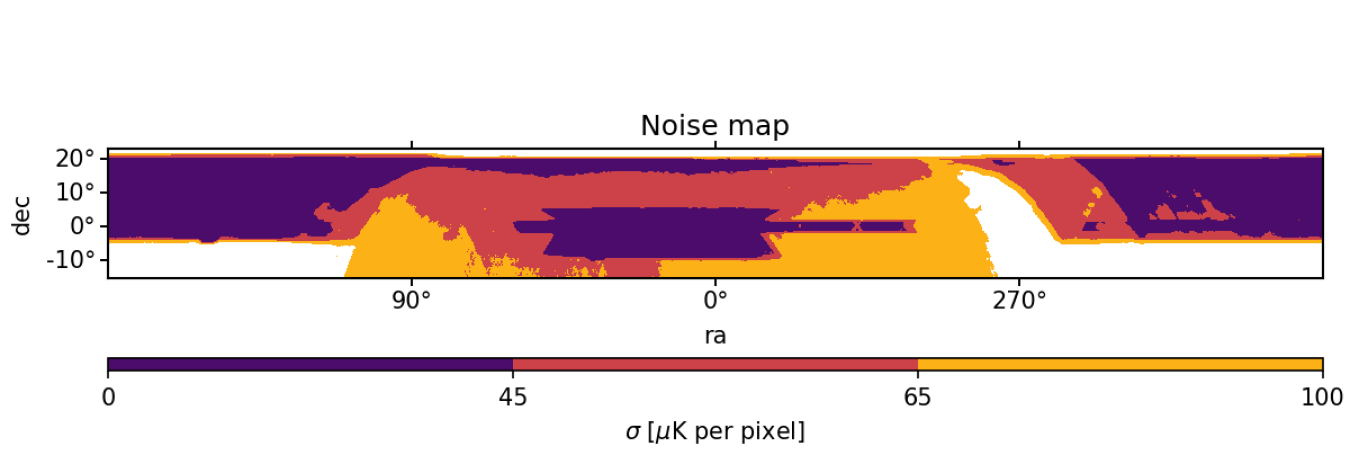
Figure 1: Top: The ACT + Planck map used for the DR5 f150 analysis with the overlapping 343,647 SDSS DR15 selected sources plotted in blue over 3,700 sq. deg., and the BN and D56 areas covered by the ILC maps plotted in green and orange, respectively. Bottom: The inverse white noise variance map associated with the DR5 f150 coadded ACT+Planck map highlighting regions representing a noise equivalence of 45 and 65 $\mu$K per pixel (with a 0.5 arcmin resolution plate Carré projection), which were used to cut the SDSS sample for the DR5 f150 analysis. The orange and yellow regions of higher noise overlapped with 27$\%$ of the DR15 sample. Results are shown for the more conservative 45 $\mu$K per pixel inverse white noise variance map cut, shown in purple. We performed an equivalent cut for the DR5 f090 map and analysis.

While the kSZ effect has an amplitude proportional to both the total cluster gas mass and the cluster’s line-of-sight velocity, it is independent of the gas temperature. When both the tSZ and kSZ effects are measured for the same sample of sources and the optical depth (and thus the total cluster gas mass) is modeled from the tSZ data, the combination can be used to convert the pairwise momentum Hand et al. (2012) measured from the kSZ effect into pairwise velocity, which in turn can be used to constrain cosmological parameters, such as the sum of the neutrino masses Mueller et al. (2015, 2015).

To use tSZ measurements to probe cluster properties, we must extract the tSZ signal from the microwave sky at high significance. Cleaning the tSZ signal from sources of contamination such as competing astrophysical and cosmological signals, instrumentation and atmospheric noise, and dusty galaxy and synchrotron emission can be a challenge. Recent efforts by the Atacama Cosmology Telescope (ACT) Marriage et al. (2011); Hasselfield et al. (2013); Hilton et al. (2018); Aghanim et al. (2019), South Pole Telescope (SPT) Staniszewski et al. (2009); Bleem et al. (2015), and Planck Collaborations Planck Collaboration (2020) have utilized wide-field multi-frequency data to produce measurements of the tSZ effect in CMB data. Heritage for both tSZ stacking and multifrequency dust reconstruction in ACT data includes multiple recent publications Fuzia et al. (2020); Gralla et al. (2014); Su et al. (2017).

In this work we use multi-frequency CMB temperature maps Naess et al. (2020) (Figure 1) from ACT (Data Release 5, DR5) and Planck data, along with component-separated Compton-$y$ maps Madhavacheril et al. (2020) (DR4) to extract our tSZ signals. We perform aperture photometry (AP) on stacked $18^{\prime}\times 18^{\prime}$ map cutouts (submaps) centered on sources from the Sloan Digital Sky Survey (SDSS) Baryon Oscillation Spectroscopic Survey (BOSS DR15 Aguado et al. (2019)) in luminosity selected bins. We bin by luminosity to target the highest signal-to-noise SZ measurements and enable comparisons between independent bins of sources with differing average masses. We select 343,647 luminous red galaxies (LRGs) from the DR15 catalog based on an inverse white noise variance map cut, point source mask, and Planck Galactic plane mask used in the production of the 2015 Planck Compton-$y$ map Planck Collaboration (2016a). We then clean the tSZ signals by removing contaminating emission from dusty galaxies. We convert these tSZ signals to estimates of optical depth, $\bar{\tau}$, by using a hydrodynamical model Battaglia (2016).

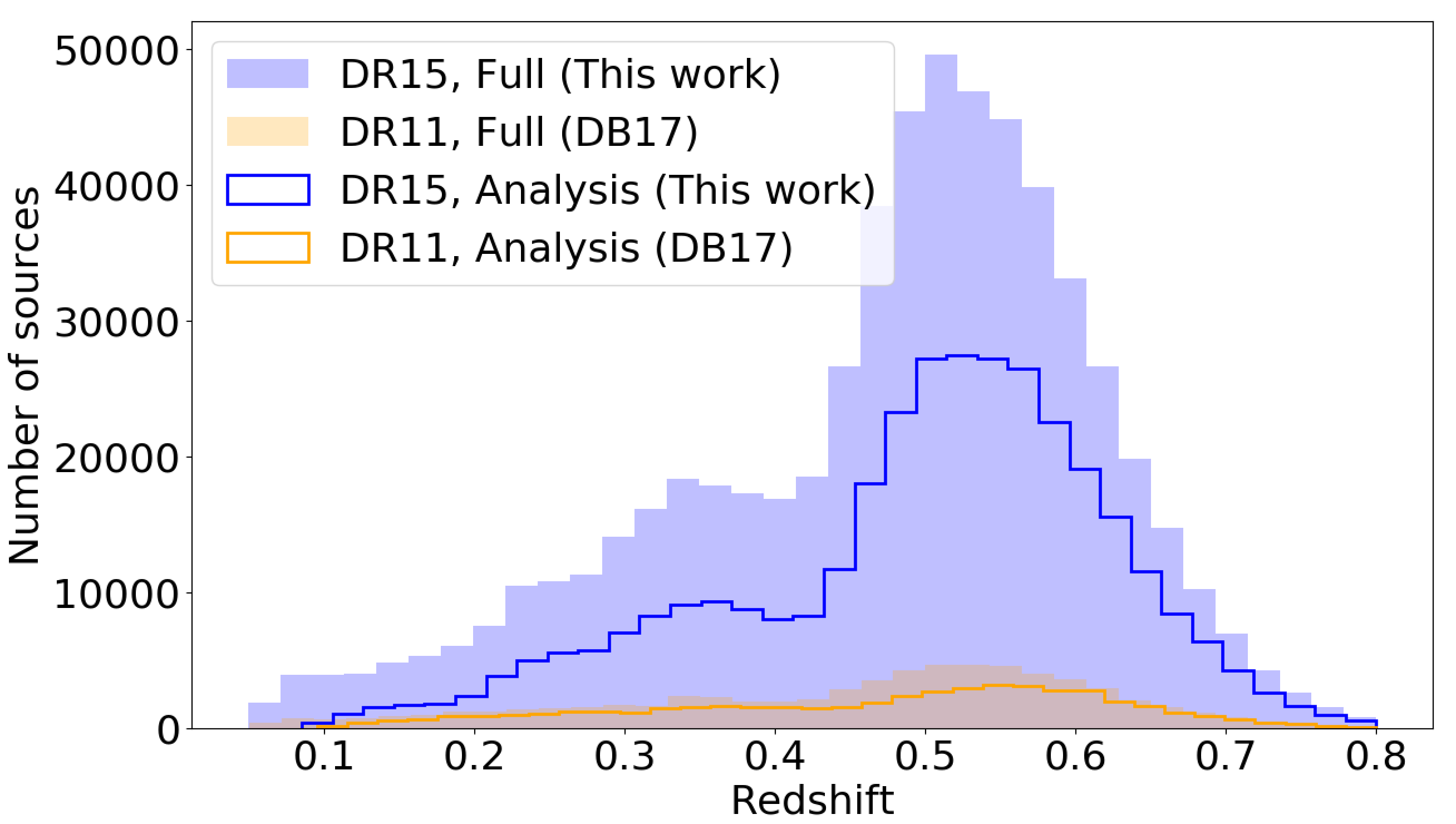
Figure 2: The SDSS DR15 redshift distribution for the 602,461 total galaxy sample and selected 343,647 galaxy sample for analysis overlapping with the ACT+Planck DR5 map, as compared to the $\sim$9 and $\sim$7 times fewer DR11 galaxies overlapping with the ACT DR3 area and those used for the 2017 result (DB17), respectively.

In a companion paper, Calafut et al. 2020 (henceforth C21) Calafut et al. (2021), we report a measurement of the pairwise kSZ signal using the same datasets described here to measure the kSZ effect at $>5\sigma$, a significant improvement over our previous results (De Bernardis et al. 2017, henceforth DB17 De Bernardis et al. (2017)). Previous measurements using the pairwise estimator Ferreira et al. (1999) have been reported by the Planck collaboration using galaxies from SDSS Planck Collaboration (2016b), and the South Pole Telescope collaboration using galaxies from the Dark Energy Survey Soergel et al. (2016). In C21, we obtain optical depth estimates by fitting to an analytical kSZ signal model. In this work, we compare these estimates to $\bar{\tau}$ estimates obtained through tSZ measurements.

In 2011, Hand et al. presented a measurement of the tSZ effect in ACT maps using a matched-filtering method with an assumed profile Hand et al. (2011). In DB17, a 600 deg² map from ACT Data Release 3 (DR3) was analyzed in combination with sources from the SDSS DR11 galaxy catalog (Figure 2) also using a matched filter for the tSZ signal extraction. Then $\bar{\tau}$ was estimated from the same hydrodynamical simulations used in this work. In this work, we adopt the aperture photometry approach for both the tSZ and kSZ analysis and estimate both the tSZ uncertainties and kSZ covariance matrix using jackknife estimates for consistency. The tSZ results presented here are consistent with those in DB17, with smaller uncertainties. The details of the kSZ analysis that differ between this work and DB17 are discussed in C21. Although our galaxy samples are different than those in Hand et al. 2011 Hand et al. (2011), our results are statistically consistent with those results for bins with similar average luminosity.

A pair of contemporary papers from ACT, Amodeo et al. 2020 (A20) Amodeo et al. (2020) and Schaan et al. 2020 (S20) Schaan et al. (2020), use the same ACT DR5 maps Naess et al. (2020) or component-separated maps Madhavacheril et al. (2020) as are used here and in C21, but with a different galaxy sample, to focus on the radial dependence of the kSZ and tSZ signals, i.e., on the baryon profiles. Rather than the pairwise estimator used in C21, S20 uses the velocity reconstruction kSZ estimator, which is convenient for measuring the baryon density profile. To obtain a complete picture of the gas thermodynamics, A20 and S20 stack on the CMASS and LOWZ galaxy samples Ahn et al. (2014), for which clustering and galaxy lensing measurements are available. Because the galaxy samples are different in this work than in A20 and S20, and have different host halo masses, the results from these papers are not directly comparable to ours; however the rough signal-to-noise ratios obtained are comparable. The promise of the pairwise kSZ estimator used in C21 lies in its potential for measurements of the pairwise velocity, if the optical depths of the sources are known. In this paper, we investigate methods of constraining the optical depth. Overall, these various papers are complementary, and highlight the wealth of information in joint kSZ and tSZ measurements.
In Section II we describe the ACT+Planck maps we analyze, and discuss the selection and binning of the SDSS data used for this work. In Section III we summarize our aperture photometry filtering approach towards extracting tSZ signals from our maps and measuring the average Compton-$y$ within our 2.1^′ aperture, $\bar{y}$. We describe how we use a scaling relation from hydrodynamic simulations to convert these measurements of $\bar{y}$ into estimates of halo optical depth, $\bar{\tau}$. We explore dust and beam corrections and possible systematic effects in Section III.C. We calculate theoretical estimates for these halos in Section III.E in order to compare with our estimates. In C21, kSZ-based estimates of $\bar{\tau}$ are obtained for the same dataset. We discuss this in Section III.D. We present the tSZ $\bar{y}$ measurements for each bin and estimated $\bar{\tau}$ values from the tSZ and kSZ results in Section IV. The optical depth estimates from the kSZ signals from C21 and tSZ signals from this work are compared with the theoretical estimates and with one another in Section IV.C. We assume the Planck cosmology for a flat universe Planck Collaboration (2016a): $\Omega_{b}h^{2}=0.02225$, $\Omega_{c}h^{2}=0.1198$, $H_{0}=67.3$ km/s/Mpc, $\sigma_{8}=0.83$, $n_{s}=0.964$. Combining the SZ measurements provides a step towards using observations to refine our models of galaxy formation and feedback, leading towards an empirical $\bar{y}$-$\bar{\tau}$ relationship free of the assumptions required in current simulations.

II Data

				DR5 f150, DR5 f090			DR4 ILC
Bin	Luminosity cut/$10^{10}L_{\odot}$	$M_{\mathrm{vir}}$ cut/$10^{13}M_{\odot}$	$\langle M_{*}\rangle/10^{11}M_{\odot}$	N	$\langle L\rangle/10^{10}L_{\odot}$	$\langle z\rangle$	N	$\langle L\rangle/10^{10}L_{\odot}$	$\langle z\rangle$
L43∗	$L>4.30$	$M>0.52$	2.21	343647	7.4	0.49	190551	7.4	0.50
L61∗	$L>6.10$	$M>1.00$	2.61	213070	8.7	0.51	118852	8.7	0.51
L79∗	$L>7.90$	$M>1.66$	3.17	103159	10.6	0.53	57828	10.6	0.54
L98	$L>9.80$	$M>2.59$	3.84	46956	12.8	0.56	26308	12.8	0.57
L116	$L>11.60$	$M>3.70$	4.50	23504	15.0	0.58	13277	15.0	0.59
L43D∗	$4.30<L<6.10$	$0.52<M<1.00$	1.57	130577	5.2	0.48	71699	5.2	0.48
L61D∗	$6.10<L<7.90$	$1.00<M<1.66$	2.08	109911	6.9	0.48	61024	6.9	0.48
L79D	$7.90<L<9.80$	$1.66<M<2.59$	2.61	56203	8.7	0.51	31520	8.7	0.52
L98D	$9.8<L<11.60$	$2.59<M<3.70$	3.18	23452	10.6	0.54	13031	10.6	0.55

Table I: Luminosity bin labels (the ^∗bins are also analyzed in C21) and cuts (Appendix B), equivalent halo mass cuts, average stellar mass per bin, Number of sources (N), average luminosity ($\langle L\rangle$), and average redshift ($\langle z\rangle$) per luminosity bin for the final DR15 samples used in the DR5 f150, DR5 f090, and ILC Compton-$y$ map analyses. These samples have the noise cut, point source masks and Galactic plane mask applied. The samples differ between the coadded and ILC maps due to the difference in footprints of the two maps, with the ILC maps covering a smaller area on the sky.

II.A ACT data

This analysis uses a component separated internal linear combination (ILC) Compton-$y$ map, referred to as the DR4 ILC map, covering the BN (1633 sq. deg.) and D56 (456 sq. deg.) regions (see Figure 1). The ILC map is comprised of two seasons of observations with the ACTPol receiver Thornton et al. (2016) (ACT DR4) Madhavacheril et al. (2020). In C21, the DR4 ILC map used for the kSZ analysis is a CMB+kSZ map. The ILC approach was designed to account for the anisotropic noise found in ground-based CMB experiments. The ILC method combines multi-frequency data from Planck and ACT and constructs wide-area, arcminute-resolution component-separated maps of CMB temperature and the tSZ effect. CIB-deprojected Compton-$y$ maps are also available, but were not analyzed in this work due to their higher noise. Additionally, ACT DR5 single frequency data at 150 and 98 GHz is coadded with data from Planck at 100 and 143 GHz to cover about 21,100 sq. deg. of sky (3,700 sq. deg. of which overlaps with the SDSS data sample) Naess et al. (2020). These maps are referred to as the DR5 f150 and DR5 f090 maps. While the DR5 data has the highest signal-to-noise ratio, the DR4 ILC results serve to check consistency with a map that already combines the multi-frequency information. A higher signal-to-noise ILC map for the DR5 data is not yet available and so was not analyzed here, but will be useful for future measurements. The beams have FWHM = 1.3^′, 2.1^′, and 1.6^′ for the DR5 f150, DR5 f090 and DR4 ILC maps, respectively, with associated uncertainties of several percent Naess et al. (2020).

The inverse white noise variance map associated with the DR5 data is used for cutting the SDSS data sample (Section II B) and for weighting (Section III B). For the ILC analysis, the DR5 f090 inverse white noise variance map is used for weighting as it best estimates the noise properties in the ILC map. Figure 1 shows the ACT+Planck map overlaid with the selected 343,647 sources from the SDSS DR15 catalog.

For the tSZ measurements, submaps are stacked on the locations of galaxies from the public Sloan Digital Sky Survey Large Scale Structure DR15 catalog from the BOSS survey Dawson et al. (2013). The tSZ signal from the CMB map is measured at the positions of these objects. We assume that higher luminosity optical galaxies trace more massive halos. Systematic effects associated with this assumption are discussed in the context of these data in C21, and have been previously explored for precursor data in Calafut et al. (2017). The assumption that each galaxy traces one halo is discussed in Section III.C.

II.B SDSS data

The 602,461 DR15 LRGs overlapping with the DR5 f150 ACT+Planck map were selected for use in this analysis through a luminosity cut, a cut based on the CMB map noise level, point source masks, and a Galactic plane mask. The catalog was downloaded from the SDSS SkyServer using the query presented in Appendix A. The full catalog, with flags for the cuts described below, is publicly available. The luminosities of the sources are calculated based on their (multiband) de-reddened SDSS composite model magnitudes and K-corrected using the k_correct Blanton and Roweis (2007) software according to the luptitude to flux conversion outlined in Lupton et al. (1999). The DR15 luminosities of the selected sources range from $4.30\times 10^{10}L_{\odot}$ to $2.61\times 10^{12}L_{\odot}$ with an average luminosity of $7.38\times 10^{10}L_{\odot}$. Luminosity bins for joint tSZ and kSZ analyses with C21 were chosen to match two of the luminosity cuts from DB17 ($L=7.9\times 10^{10}L_{\odot}$ and $L=6.1\times 10^{10}L_{\odot}$) as well as one lower luminosity cut ($L=4.3\times 10^{10}L_{\odot}$). The three disjoint bins based on these cuts were selected to have roughly equal spacing, and such that each bin has over 100,000 galaxies that pass cuts for analysis with the DR5 maps (Table I). The cumulative luminosity bins include the highest signal-to-noise SZ measurements, while the disjoint bins enable comparisons between independent bins. Since the tSZ signal-to-noise ratio is higher for high mass halos, we also perform the tSZ analysis for the two highest mass bins from DB17 (L98 and L116) which are not studied in C21. A plot of the luminosity distribution and bins is shown in Appendix B.

After we selected luminosity bins and applied the minimum luminosity cut, which removed 80,162 lower luminosity sources from the sample, we performed an inverse white noise variance cut. Figure 1 shows the inverse white noise variance map that was used to explore cuts in the DR15 sample. Initially two different cuts were studied (45 and 65 $\mu$K per pixel). The more conservative cut of 45 $\mu$K per pixel was selected for all subsequent analyses based on a signal-blind uncertainty analysis which compared the jackknife error bars on the aperture photometry (AP) analysis for the samples cut by 45 $\mu$K per pixel, 65 $\mu$K per pixel, and no noise cut. The 45 $\mu$K per pixel cut removes 27$\%$, or 140,209 sources from the overlapping sample and improves the jackknife error bars as compared to no noise cut.

Galactic plane masking was then performed with the mask used in the production of the 2015 Planck Compton-$y$ map to reduce Galactic contamination Planck Collaboration (2016a). The 50$\%$ mask was selected to conservatively cut sources from the Galactic plane region of the ACT+Planck map, resulting in a cut of 26,521 additional sources from the DR15 sample.

To mask point sources we first used the two source masks developed for Choi et al. 2020 Choi et al. (2020). For the lowest noise D56 region a 15 mJy point source mask was applied, and for the higher noise regions a 100 mJy mask was applied. Together these masks removed an additional 11,922 sources from our sample, leaving us with a final selected sample of 343,647 sources after all masks and cuts are applied.

Figure 2 shows the redshift distributions of the 343,647 DR15 galaxies overlapping with the ACT+Planck map after the luminosity, inverse white noise variance map, Galactic plane mask and point source mask cuts. The 67,938 DR11 sources overlapping with the coadded ACT DR3 map used in our 2017 result are also shown for comparison (DB17 De Bernardis et al. (2017)). The redshifts range from $0.08$ to $0.8$ with an average reshift of $0.49$ for the DR15 catalog.

Histograms of the luminosities depicting cuts and bins are provided in Appendix B. The properties of each luminosity-selected bin are summarized in Table I. The mean stellar masses are estimated from the mean luminosities assuming $M_{*}/L=3.0$ as predicted by the Chabrier IMF Chabrier (2003) and discussed in Kravtsov et al. (2018); Bell and de Jong (2001); Bell et al. (2003); Bernardi et al. (2010). The mean halo masses are derived from the $M_{*}-M_{vir}$ relation from abundance matching as described in Kravtsov et al. (2018). Abundance matching is a statistical technique to model the correlations between galaxy and halo properties based on mapping galaxies to dark matter halos of the same number density in the universe.

The same mass cuts and average redshifts of the sources reported in Table I are used when calculating the linear model prediction from the kSZ measurements in C21.

III Analysis

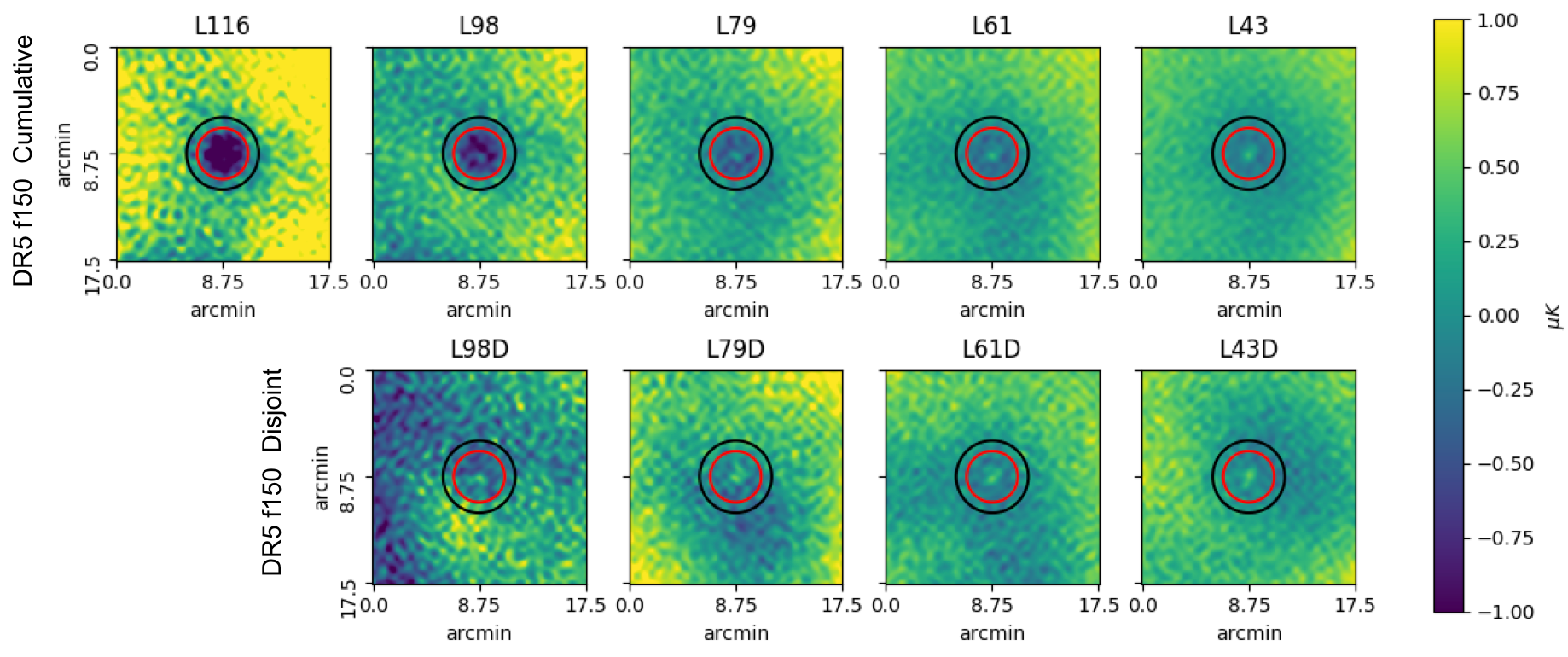
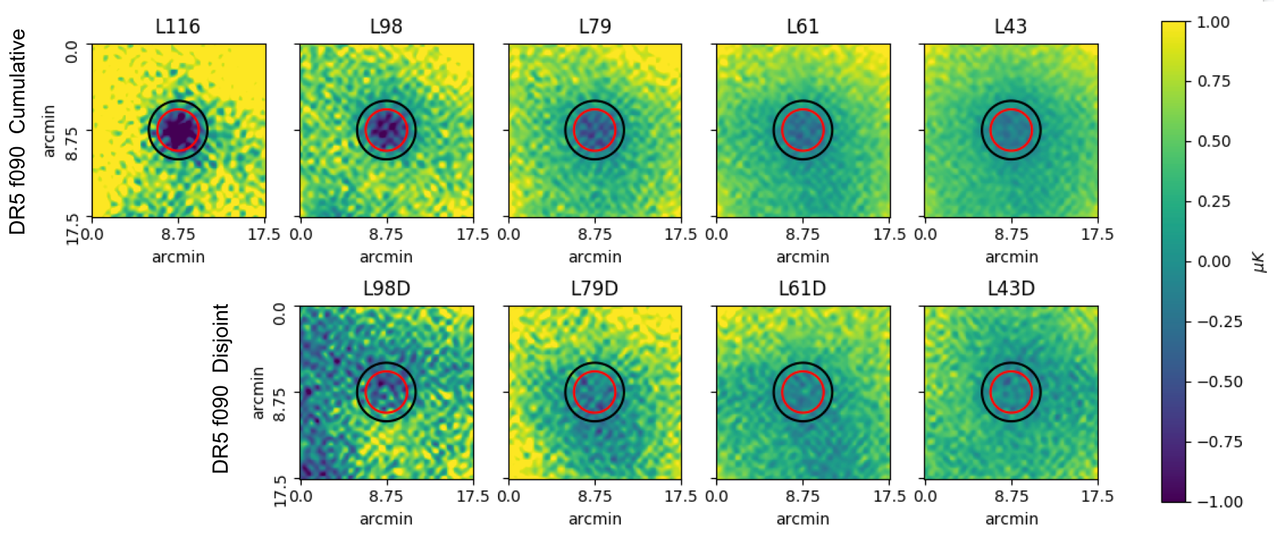
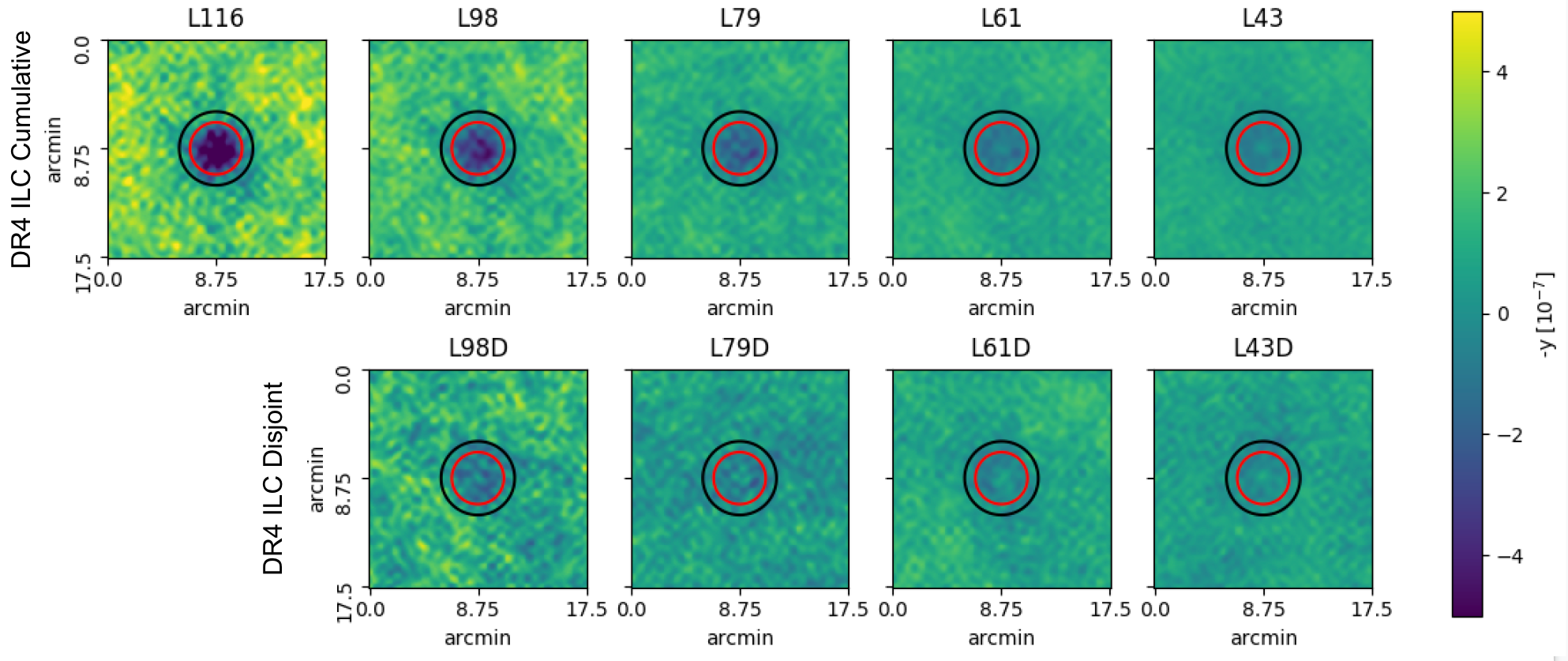
Figure 3: Stacked raw submaps for the five cumulative (top) and four disjoint (bottom) luminosity bins as defined in Table I, for the DR5 f150 map (top two rows, in differential units of CMB temperature which are calibrated to Planck Naess et al. (2020)), the DR5 f090 map (middle two rows, in the same units as the top two rows) and the DR4 ILC Compton-$y$ maps (bottom two rows, in negative units of $y$ to better compare to the coadded maps). The submaps represent the weighted average submaps of the sources in a given bin, where the weight for each source is taken to be the average value inside the accompanying $R_{1}=2.1$ submap in the inverse white noise variance map. The sub-0.5^′-scale structure in the submaps is an artifact of the sub-pixel interpolation and is not physical. The maps are normalized with the average value within the AP annulus, such that the mean of the pixels in the annulus in these maps is equal to zero. The apertures used for the tSZ and kSZ AP are drawn, where $R_{1}=2.1^{\prime}$ (red) and $\sqrt{2}R_{1}$ (black). Radial averages of these submaps are plotted in Figure 4. A central bright spot due to dust on approximately the beam scale can be seen across luminosity bins in the DR5 f150 submaps, but not the DR5 f090 submaps. Dust contamination of the DR4 ILC maps is more subtle, but can be noticed in radial average plots (Figure 4).

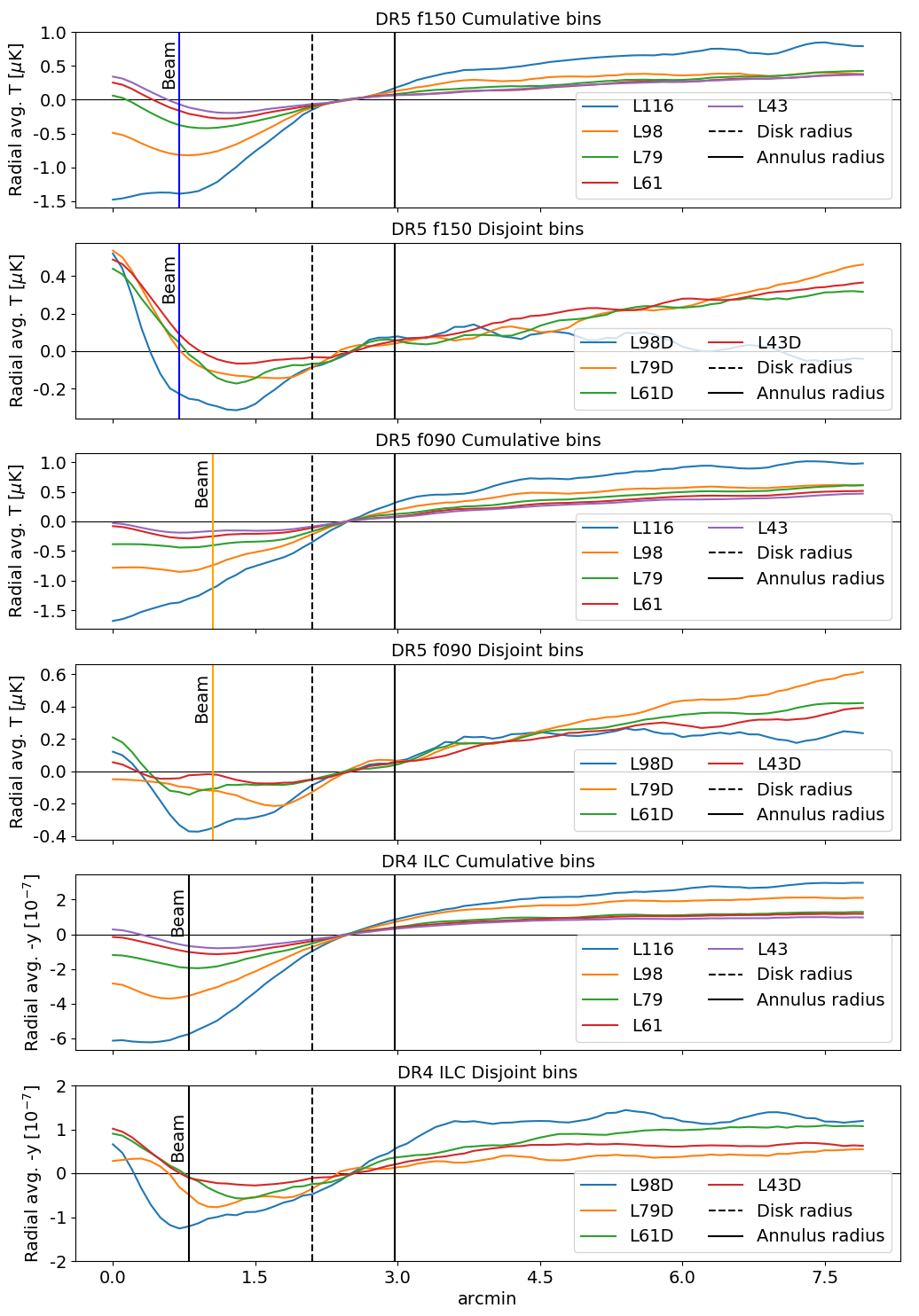
Figure 4: Radial average of the stacked submaps, which have been repixelized to 0.1^′ per pixel, normalized to the average annulus value, for each luminosity bin, for the DR5 f150 and DR5 f090 coadded maps as well as the DR4 ILC map, shown for illustrative purposes only. The native units of the DR5 f150 and DR5 f090 maps are in $\mu\mathrm{K}$ and the DR4 ILC maps in $y$. Negative $y$ is plotted here to compare with the decrements present in temperature. The aperture photometry disk radius is plotted as a vertical black dashed line, and the annulus outer radius is plotted as a vertical solid black line. The beam radius is plotted as a blue vertical line for DR5 f150, an orange vertical line for DR5 f090, and a black vertical line for the effective DR4 ILC beam. A central “bright spot” is observed in nearly all but the most luminous bin, and is attributed to dust emission. Due to this effect, we studied the core-excised AP approach for the DR5 f150 and DR5 f090 analysis (Sections III.B, III.C).

We use aperture photometry (AP) to filter the Compton-$y$ and DR5 f150 maps and extract the tSZ signals by stacking on source-centered submaps. The same 2.1^′ AP filter is used in the kSZ analysis in C21. This approach to comparing estimated optical depths is an improvement over the 2017 result in which a matched filter was used for the tSZ analysis while AP was used for the kSZ analysis.

III.A Filtering CMB maps

We select submaps of 18${}^{\prime}\times 18^{\prime}$ (about three times larger than the outer diameter of the AP annulus) of pixel size 0.5^′, interpolate in the Fourier domain with a pixel size of 0.1^′ per pixel, and reproject to a coordinate system centered at the galaxy center position using pixell. A comparison between different pixelization approaches is discussed in C21 Appendix A, and we use here the same approach adopted in C21. On each source-centered submap, we draw an aperture of $R_{1}=2.1^{\prime}$ located at the central coordinate in RA and DEC provided by the DR15 catalog. The signal associated with the sources is taken to be the average within this aperture, minus the average of the pixels within an annulus of inner radius $R_{1}=2.1^{\prime}$ and an outer radius of $\sqrt{2}R_{1}$. The 2.1^′ size of this annulus was selected to correspond to $\sim$0.8 Mpc based on the average angular diameter distance for the source sample and assumed cosmology (Section I). An associated weight for each source is assigned by taking the average within a $R_{1}=2.1^{\prime}$ disk centered on the same source position on a 18${}^{\prime}\times 18^{\prime}$ submap taken from the inverse white noise variance map. This value is used for weighting the signals in the tSZ analysis.

III.B tSZ signal extraction

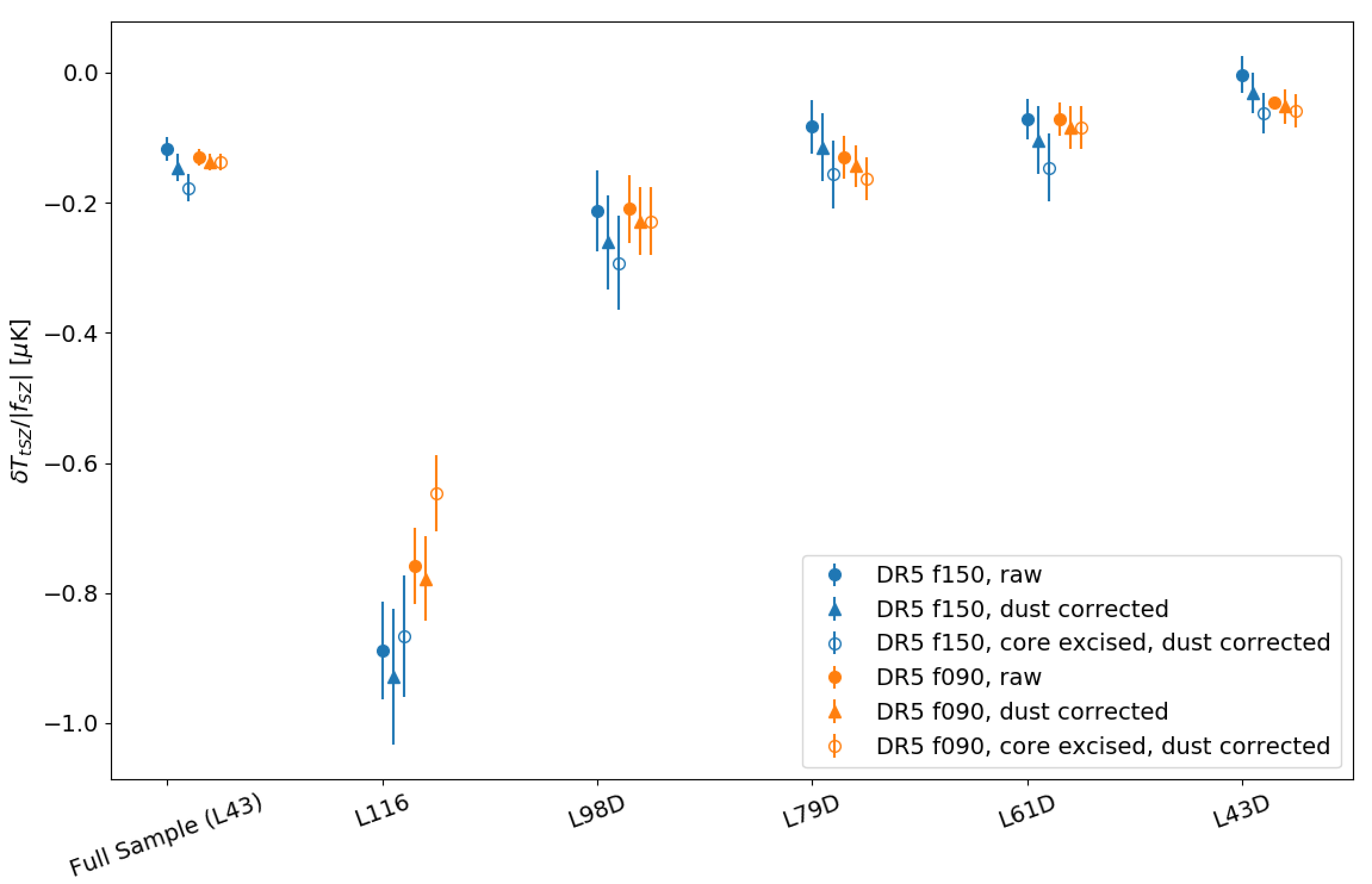
Figure 5: Aperture photometry tSZ signals in units of temperature rescaled by $|f_{\rm SZ}|$ (Equation 2) for disjoint luminosity bins and the full analysis sample, with 1$\sigma$ jackknife estimated uncertainties, for the DR5 f150 and DR5 f090 maps. Raw results using the 2.1^′ radius are compared to results after Herschel dust correction (Section III.C) and the removal of the pixels within a beam-scale radius (0.7^′ for the DR5 f150 map and 1.1^′ for the DR5 f090 map, Section III.B). The DR5 f090 results shown have been beam corrected (Section III.B). The Herschel dust correction has a small effect on the temperature signals and lowers signal-to-noise for the DR5 f090 map due to the relatively large error bars on the dust estimates which are propagated into the uncertainties on tSZ signal. The “core-excised” AP approach removes a noticeable amount of tSZ signal in the L116 bin, as there is less dust contamination apparent on the beam scale in the stacked submaps for this bin as compared to the lower luminosity bins (Figure 4). For the most part, it has less than a $1\sigma$ effect on the tSZ signals, and is not included in the rest of this analysis. The dust corrected (filled triangle) results are propagated through to our comparisons of optical depth estimates.

We stack on the positions of DR15 sources in the nine luminosity bins listed in Table I to measure the average $\delta T_{SZ}$ in differential CMB temperature units from the DR5 f090 and DR5 f150 maps, and the average Compton-$y$ for the DR4 ILC map. Round number luminosity cuts were chosen to yield five cumulative and disjoint luminosity bins, before any cuts were made to the DR15 sample, or any analyses were run. The weighted averages of the stacked submaps for each bin are shown in Figure 3, and the radial averages of these submaps are plotted in Figure 4. The signal associated with each source in a bin is taken to be the average of the $\langle{\rm disk}\rangle-\langle{\rm ring}\rangle$ values per source, weighted by the associated average inverse variance weight per source. The presence of dust emission on angular scales comparable to or less than the beam size is visible in all the maps analyzed, but is most prominent in the DR5 f150 map (Figures 3-4). We study the impact of discarding the pixels within the beam radius from our analysis, as discussed further in Section III.C. This “core-excised” AP method removes the SZ signal within the beam radius along with the dust emission; it has a small (generally $<1\sigma$) effect on the tSZ signals (Figure 5), so it is not adopted for the final analysis. The 2.1^′ AP signals are then averaged in each bin to obtain a stacked tSZ signal, $\delta T_{\rm tSZ}$. The uncertainty associated with the stacked tSZ signal for each bin is obtained using a jackknife estimation method over the sources with 2,000 iterations per bin.

We correct the $\delta T_{\rm tSZ}$ and $\bar{y}$ estimates obtained from the DR5 f090 map to account for the larger DR5 f090 beam (FWHM=2.1^′) compared to the DR5 f150 map (FWHM=1.3^′) Naess et al. (2020). We also correct the $\bar{y}$ estimates from the DR4 ILC map which has an effective beam corresponding to a 1.6^′ FWHM Gaussian Madhavacheril et al. (2020). We compute the beam correction factors as follows: we consider a fiducial pressure profile for the average virial mass ($M_{\mathrm{v}ir}$) in each bin Battaglia et al. (2012); we derive three estimates of the Compton-$y$ signal in a 2.1^′ AP filter, convolved with the f150 and f090 beams from Naess et al. (2020) and with a 1.6^′ FWHM Gaussian beam, using Mop-c GT (see Amodeo et al. (2020) for a detailed description on how the projection from pressure to Compton-$y$ profile and the beam convolution are implemented). We find an AP beam correction of 31% for the DR5 f090 measurements, and a beam correction of -5% for the DR4 ILC measurements. Thus, the DR5 f090 $\delta T_{\rm tSZ}$ measurements are multiplied by 1.3, which propagates into the DR5 f090 Compton-$y$ estimates and resulting analyses, and the DR4 ILC $\bar{y}$ measurements are multiplied by 0.95. The value for the correction changes negligibly across luminosity bins, and is insensitive to our estimate of $M_{\mathrm{v}ir}$ (the change in factor is $\sim 1\%$ if we vary $M_{\mathrm{v}ir}$ in our mass range). While Figures 3 and 4 show the raw data, the DR5 f090 and DR4 ILC data in the rest of this work are multiplied by these factors. We note that because the f150 beam is not exactly Gaussian, but features secondary lobes, we get a negative ($<1$) ILC correction, contrary to what we would expect given the larger ILC FWHM.

For the DR5 f150 and DR5 f090 analysis, we then estimate the aperture-averaged Compton-$y$ parameter $\bar{y}$ from this temperature signal and use a theoretical relation between optical depth and $\bar{y}$ from hydrodynamical simulations to infer the optical depth Battaglia (2016). To obtain the Compton-$y$ parameter we follow the steps detailed in Hasselfield et al. (2013) and DB17. The tSZ temperature signal is related to the Compton-$y$ parameter by

$$\frac{\delta T_{\rm tSZ}(\theta)}{T_{\rm CMB}}=f_{\rm SZ}\hskip 3.0pty(\theta),$$ (1)

where $y(\theta)$ is the Compton parameter at a projected angle $\theta$ from the cluster center and, in the non-relativistic limit, $f_{\rm SZ}$ depends on observed radiation frequency:

$$f_{\rm SZ}=\Big{(}x\frac{e^{x}+1}{e^{x}-1}-4\Big{)}.$$ (2)

Here, $x=h\nu/k_{B}T_{\rm CMB}$ Itoh et al. (2000). The effective band centers vary based on sky position in the coadded maps, so the median values of the SZ-weighted band centers are chosen for our analysis. The appropriately weighted band center frequencies are 97.8 and 149.6 GHz for the DR5 f090 and DR5 f150 maps, respectively, so $f_{\rm SZ,f090}=-1.53$ and $f_{\rm SZ,f150}=-0.958$ Hilton et al. (2020). Relativistic corrections are negligible for this sample mass and can safely be excluded Nozawa et al. (2006). We assume the ACT-based band center frequencies because the ACT measurements dominate over those from $Planck$ at our scales Naess et al. (2020). These frequencies are associated with a 2.4 GHz uncertainty, and detailed bandpass considerations could carry a larger impact (at the few percent level). However, each of these has a small effect on $\bar{y}$ compared to our uncertainties. For each luminosity bin, $\bar{y}$ is obtained from the AP temperature signal $\delta T_{\rm tSZ}$ via equation (1).

A jackknife approach is used to estimate the uncertainties associated with the binned tSZ signals and the covariance matrix for the kSZ analysis. We split the sample of sources into $N$ smaller subsamples and remove one subsample at a time, calculating the weighted average for each bin on the summed $N-1$ subsamples to obtain $N$ realizations of the computation. The jackknife method has the advantage of being self-contained and not requiring external information such as simulated CMB maps. We have varied $N$ to check the convergence of the jackknife algorithm, selecting the value that provided a stable significance against variations of $N$. For the tSZ analysis, a choice of $N=2000$ was conservative.

In simulations with AGN feedback, Battaglia Battaglia (2016) finds the relationship between $\bar{y}$ and optical depth to be

$$\ln(\bar{\tau})=\ln(\tau_{0})+m\ln(\bar{y}/10^{-5})$$ (3)

where $\ln(\tau_{0})=-6.40$ and $m$ = $0.49$ at z = 0.5. We use this to estimate $\bar{\tau}$ from our $\bar{y}$ measurements. The systematic error bars on $\bar{\tau}$ from the $\bar{y}$-$\bar{\tau}$ relationship are calculated by using the Monte Carlo method taking into account the estimated $4\%$ systematic uncertainty on $\ln(\tau_{0})$ and 8$\%$ on $m$. The systematic uncertainties on $\ln(\tau_{0})$ and $m$ were estimated in Battaglia (2016) by taking the largest relative differences between the radiative cooling and AGN feedback models used for Equation 3.

A null test was performed by stacking the ILC sample on a simulated ILC CMB-only map. This test served as a check of our pipeline and jacknife estimates. The same pipeline used in the ILC analysis was used to measure the Compton-$y$ parameter in the simulated CMB map for all luminosity bins in Table I, print stacked submaps as in Figure 3, and plot radial averages as in Figure 4. The Compton-$y$ results for the simulated CMB map were consistent with zero within $1\sigma$ for all luminosity bins. The stacked submaps were also consistent with the same noise level as estimated using the jackknife uncertainty estimations.

III.C tSZ systematic effects

Several systematic effects have the potential to impact the amplitude of the measured tSZ signals. One potential systematic for the tSZ measurement is the light emitted from star-forming SDSS galaxies in the optical/UV that is absorbed by dust grains and re-emitted in the infrared/sub-mm. To account for this, for both coadded maps we fit a model of the spectral energy distribution (SED) to Herschel data from one large extragalactic survey that overlaps with SDSS, the Herschel Astrophysical TeraHertz Large Area Survey (H-ATLAS) Eales et al. (2010), in the three fields GAMA-9, GAMA-12 and GAMA-15. We use the three SPIRE photometric bands centered at 250 $\mu$m, 350 $\mu$m, and 500 $\mu$m. Table II reports the number of galaxies in the SDSS sample overlapping with the Herschel map areas for each luminosity bin analyzed.

We apply an aperture photometry filter at the position of each galaxy in our SDSS sample with aperture 2.1^′ and stack the signal measured from the Herschel maps following the approach described in A20 Amodeo et al. (2020) (see their Appendix B). Using these measurements, we fit a model of the dust SED described by the following modified blackbody:

$$I(\nu)=~{}A_{\rm d}\left(\frac{\nu(1+z)}{\nu_{0}}\right)^{\beta_{\rm d}+3}\frac{e^{(h\nu_{0}/k_{B}T_{\rm d})}-1}{e^{(h\nu(1+z)/k_{B}T_{\rm d})}-1}\,,$$ (4)

where $\nu_{0}=857$ GHz is the rest-frame frequency at which we normalize the dust emission, $A_{\rm d}$ is the amplitude of the dust emission in [kJy/sr], $\beta_{\rm d}$ is the dust spectral index, and $T_{\rm d}$ is the dust temperature in K. We assume flat priors for the the dust amplitude and temperature parameters in the ranges: $0.05<A_{\rm d}~{}{\rm[kJy/sr]}<5$, $10<T_{\rm d}~{}{\rm[K]}<40$. Given the degeneracy among the parameters, we assume a Gaussian prior for the emissivity index centered on 1.2 and with standard deviation of 0.1, truncated in the range $1<\beta_{\rm d}<2.5$, as in Amodeo et al. (2020). We obtain constraints on the model parameters using an MCMC sampler (emcee Foreman-Mackey et al. (2013)) to estimate the posterior probability function. Our best-fit values for the dust temperature are in the range $21<T_{\rm d}~{}{\rm[K]}<30$ across the luminosity bins, with $1\sigma$ uncertainties of $\sim 30$%, and $\beta_{\rm d}=1.2\pm 0.1$ consistent with our prior. We finally infer the amount of dust emission at 150 GHz and 98 GHz. We report our estimates of the dust emission in $\mu$K units; these need to be removed from the tSZ signal in Table II. We obtain these values by multiplying our best fit estimates from eq. 4, with $\nu=150$ GHz and $\nu=98$ GHz, respectively, by the factor $\left(\frac{dB(\nu,T)}{dT}\right)^{-1}$, where $T=T_{\rm CMB}$ and $B$ is the Planck function, in order to convert from the Herschel map intensity units to differential CMB temperature units that match the units of our SZ measurements. Because the error bars on the dust estimates are asymmetric, the largest values for each data point are selected for the more conservative estimate of $\bar{y}/\sigma(\bar{y})$ (Figure 6).

Bin	N	Tdust,150GHz [$\mu$K]	Tdust,98GHz [$\mu$K]
L43	12726	$0.026^{+0.014}_{-0.008}$	$0.012^{+0.008}_{-0.004}$
L61	7784	$0.028^{+0.019}_{-0.010}$	$0.013^{+0.010}_{-0.005}$
L79	3858	$0.029^{+0.016}_{-0.010}$	$0.014^{+0.009}_{-0.005}$
L98	1795	$0.037^{+0.027}_{-0.014}$	$0.017^{+0.014}_{-0.007}$
L116	941	$0.043^{+0.063}_{-0.023}$	$0.021^{+0.031}_{-0.011}$
L43D	4872	$0.026^{+0.022}_{-0.011}$	$0.013^{+0.011}_{-0.005}$
L61D	3926	$0.034^{+0.037}_{-0.017}$	$0.018^{+0.023}_{-0.010}$
L79D	2063	$0.027^{+0.026}_{-0.012}$	$0.014^{+0.015}_{-0.007}$
L98D	854	$0.049^{+0.035}_{-0.021}$	$0.022^{+0.016}_{-0.010}$

Table II: Estimated dust signal and 1$\sigma$ statistical uncertainties for the DR5 f150 and DR5 f090 maps using 4 percent of the SDSS sample used in this analysis overlapping with the Herschel map areas, as computed using the method described in Amodeo et al. (2020).

In the raw data, we observe a central “bright spot” in several luminosity bins in all maps, most notably the DR5 f150 map. We attribute this to additional dust contamination at approximately the beam scale in the stacked submaps (Figure 3), as shown in the radial averages presented in Figure 4.

This apparent dust contamination is particularly present in the DR5 f150 map and is stronger than the emission estimated from Herschel. The apparent angular scale, comparable to the beam size, suggests a compact source. We explored the effect of this excess emission by using a core-excised AP approach for the DR5 maps, using an aperture photometry filter which excluded the central disk on the beam scale (Section III.B). We do not include the core-excised AP approach in our reported results or optical depth comparisons due to the small (generally $<1\sigma$) impact on the tSZ signals, to avoid biasing our results by removing the central portion of the tSZ signal, and to best compare with the results from C21. Thus, while the Herschel dust correction accounts for some of the dust present in the DR5 f150 and DR5 f090 maps, this correction is imperfect, and some contamination remains from source galaxy emission. The effects of the dust correction steps taken on the DR5 f150 and DR5 f090 analyses can be seen in Figure 5.

Another potential cause of increased uncertainty in the tSZ measurements is dust and synchrotron emission from our own galaxy. To account for this, we apply the same 50$\%$ Galactic plane mask as used in the production of the 2015 $Planck$ all-sky Compton-$y$ maps Planck Collaboration (2016a). This cut eliminated 16,977 sources after all other cuts are considered, or 6$\%$ of our final sample, and was found to have a negligible impact on our signal compared to not applying the mask. We do not expect that synchrotron emission from the SDSS galaxies themselves has a significant impact on our discussion in this work based on the core excised comparison shown in Figure 5. Future work could improve upon our results by modeling and removing dust and synchrotron emission from the LRGs.

Our $\bar{y}$ estimates include a contribution from nearby halos, known as the two-halo term (e.g. Hill et al. (2018)), which biases them high when assuming we have only one halo per source. Compared to the Battaglia (2016) simulations, our sample includes lower mass halos and our measurements include a beam, so they will have a larger two-halo contribution. We estimate this contribution using Mop-c GT (see Appendix A of Amodeo et al. (2020) for details on the implementation) and we find that our $\bar{y}$ values are biased high by a factor between 2% and 10% in the luminosity bins of interest. The two-halo bias does not significantly affect the results presented in this work, but will need to be accounted for in future higher signal-to-noise analyses.

The $\bar{y}$-$\bar{\tau}$ relationship (Equation 3) also carries associated systematics. These uncertainties were estimated based on differences between radiative cooling and AGN feedback sub-grid physics models in Battaglia (2017) Battaglia (2016). While this does not encompass the wide variety of existing sub-grid models for the ICM, the two models are very different, and contrast in their inclusion of AGN feedback Battaglia (2016). In addition to the quoted systematic uncertainty between the different models, we conjectured in DB17 that there is also uncertainty in extrapolating from the larger masses in the hydrodynamical simulations to the lower mass objects in the DR11 sample used in DB17 (Section IV.C). New hydrodynamical simulations of lower mass clusters and groups would help address this concern.

III.D kSZ signal extraction

As described in C21, the mean pairwise momentum of groups and clusters as a function of their comoving separation distance is negative at and around separations of 25-50 Mpc, implying that they are moving towards one another on average due to gravity Hamilton et al. (1991); Nityananda and Padmanabhan (1994); Juszkiewicz et al. (1999); Sheth et al. (2001). While the 3-dimensional momentum of the groups is not easily measurable, the mean pairwise momentum $p$ can be still estimated from the line-of-sight component of the momenta Ferreira et al. (1999). The kSZ signal of a given cluster is directly proportional to this line-of-sight momentum: $\delta T_{\rm kSZ,i}\propto-\mathbf{p}_{i}\cdot\mathbf{r}_{i}$, where the unstated multiplicative factors depend on the properties of the cluster (density profile, including angular extent in the sky) and on the pixel scale and angular resolution of the CMB experiment.

The significance of the kSZ measurement is determined by a fit to the analytic prediction of linear perturbation theory for the pairwise velocity Hamilton et al. (1991); Nityananda and Padmanabhan (1994); Juszkiewicz et al. (1999); Sheth et al. (2001); Bhattacharya and Kosowsky (2008); Mueller et al. (2015, 2015), rescaled by the factor $-\bar{\tau}T_{\rm CMB}/c$, where $\bar{\tau}$, the average halo optical depth of the galaxy sample used for the pairwise momentum estimator, is the free parameter of the fit.

	DR5 f150		DR5 f090		DR4 ILC
Bin	$\delta\rm{T}_{\rm{tSZ,corr.}}(\mu$K)	$\bar{y}/10^{-7}$	$\delta\mathrm{T}_{\mathrm{tSZ,corr.}}(\mu$K)	$\bar{y}/10^{-7}$	$\bar{y}/10^{-7}$
L43	-0.14 $\pm$ 0.02	0.53 $\pm$ 0.09	-0.21 $\pm$ 0.02	0.51 $\pm$ 0.06	0.54 $\pm$ 0.08
L61	-0.21 $\pm$ 0.03	0.79 $\pm$ 0.11	-0.29 $\pm$ 0.03	0.70 $\pm$ 0.07	0.78 $\pm$ 0.10
L79+	-0.32 $\pm$ 0.03	1.22 $\pm$ 0.13	-0.47 $\pm$ 0.04	1.12 $\pm$ 0.11	1.28 $\pm$ 0.14
L98	-0.57 $\pm$ 0.06	2.18 $\pm$ 0.22	-0.77 $\pm$ 0.06	1.84 $\pm$ 0.15	2.19 $\pm$ 0.22
L116	-0.89 $\pm$ 0.10	3.42 $\pm$ 0.37	-1.19 $\pm$ 0.10	2.86 $\pm$ 0.24	3.52 $\pm$ 0.34
L43D+	-0.03 $\pm$ 0.03	0.11 $\pm$ 0.13	-0.08 $\pm$ 0.04	0.20 $\pm$ 0.09	0.13 $\pm$ 0.11
L61D+	-0.10 $\pm$ 0.05	0.39 $\pm$ 0.18	-0.13 $\pm$ 0.05	0.31 $\pm$ 0.11	0.28 $\pm$ 0.12
L79D	-0.11 $\pm$ 0.05	0.41 $\pm$ 0.18	-0.22 $\pm$ 0.05	0.53 $\pm$ 0.13	0.46 $\pm$ 0.16
L98D	-0.25 $\pm$ 0.07	0.97 $\pm$ 0.27	-0.35 $\pm$ 0.08	0.85 $\pm$ 0.19	0.78 $\pm$ 0.28

Table III: Thermal SZ results from the DR5 f150, DR5 f090, and DR4 ILC map analyses, along with 1$\sigma$ jackknife uncertainty estimates. Dust-corrected stacked tSZ signals $\delta T_{\rm tSZ}$ and $\bar{y}$ are given for the two coadded temperature maps, and $\bar{y}$ for the DR4 ILC Compton-$y$ map. For the DR5 f150 map, the Herschel dust correction is applied, and the uncertainties associated with these corrections are propagated into the cited jackknife uncertainties. For the DR5 f090 map, the Herschel dust correction and the f090 beam correction scaling factor are applied. The $\bar{y}$ results from the disjoint bins shared with C21 (marked as ⁺bins) are shown in Figure 8.

Figure 6: Average Compton-$y$ in the 2.1^′ aperture for the five disjoint (highest luminosity bin L116 and bin labels with suffix “D”) luminosity bins and the full source sample ($L>4.3\times 10^{10}L_{\odot}$), with jackknife estimated uncertainties, for the DR5 f150 and DR5 f090 maps after dust and beam correction (Sections III.B, III.C, Table II) and the DR4 ILC Compton-$y$ map after beam correction. The lower panel shows the signals divided by their associated uncertainties. The significance of the tSZ effect observed generally decreases for less luminous sources, as expected. The results from each of the three maps are consistent.

III.E Theoretical $\bar{\tau}$ estimate

For comparison with our measurements, we calculate theoretical estimates for the mean optical depths $\bar{\tau}_{\mathrm{theory}}$ for each of the luminosity bins. We follow the derivation in Battaglia (2016) using an NFW profile to estimate the optical depth in a given aperture,

$$\bar{\tau}_{\mathrm{theory}}=\sigma_{\textrm{T}}x_{\mathrm{e}}X_{\mathrm{H}}(1-f_{\star})f_{\mathrm{b}}\frac{M_{\mathrm{vir}}(<\theta_{2.1^{\prime}})}{d_{A}^{2}m_{p}}.$$ (5)

Here $\sigma_{\textrm{T}}$ is the Thomson cross-section, $x_{\mathrm{e}}$ is the electron fraction defined as $x_{\mathrm{e}}=(X_{\mathrm{H}}+1)/(2X_{\mathrm{H}})$, $X_{\mathrm{H}}$ is the primordial hydrogen mass fraction ($X_{\mathrm{H}}=0.76$), $f_{\star}$ is the stellar mass fraction of the halo, $f_{\mathrm{b}}$ is the universal baryon fraction ($\Omega_{\mathrm{b}}/\Omega_{\mathrm{M}}$), $m_{\mathrm{p}}$ is the proton mass, and $d_{A}$ is the angular diameter distance to mean redshift of our sample. The parameter value for $f_{\mathrm{b}}=0.157$ is set from the cosmological parameters we choose. The value for $f_{\star}$ is inferred from the stellar mass-halo mass relation from abundance matching as described in Kravtsov et al. (2018). We define the parameter $f_{\mathrm{c}}$ = $\bar{\tau}_{{\mathrm{o}bs}}/\bar{\tau}_{\mathrm{theory}}$ to compare the estimated $\bar{\tau}$ values (Table IV) to the theoretically predicted values. This parameter represents the fraction of theoretically predicted optical depth obtained by the two SZ measurements, and is of interest to compare the consistency of the two optical depth estimate methods.

		DR5 f150
	$\bar{\tau}_{\mathrm{theory}}$	$\bar{\tau}_{\rm tSZ}$	$\sigma_{\rm sys.}$		$\bar{\tau}_{\rm kSZ}$ [C21]
Bin	$[10^{-4}]$	$[10^{-4}]$	$[10^{-4}]$	$f_{\mathrm{c,tSZ}}\pm({\rm stat.,sys.})$	$[10^{-4}]$	$f_{\mathrm{c,kSZ}}$
L43∗∗	1.39	1.28 $\pm$ 0.10	0.27	0.92 $\pm$ (0.07, 0.20)	0.54 $\pm$ 0.09	0.39 $\pm$ 0.06
L61	1.77	1.55 $\pm$ 0.11	0.30	0.88 $\pm$ (0.06, 0.17)	0.69 $\pm$ 0.11	0.39 $\pm$ 0.06
L79+	2.42	1.92 $\pm$ 0.10	0.34	0.79 $\pm$ (0.04, 0.14)	0.88 $\pm$ 0.18	0.36 $\pm$ 0.07
L98	3.35	2.55 $\pm$ 0.12	0.39	0.76 $\pm$ (0.04, 0.12)
L116	4.44	3.18 $\pm$ 0.17	0.43	0.72 $\pm$ (0.04, 0.10)
L43D+	0.70	0.59 $\pm$ 0.35	0.17	0.85 $\pm$ (0.50, 0.24)	0.46 $\pm$ 0.24	0.66 $\pm$ 0.34
L61D+	1.06	1.10 $\pm$ 0.25	0.25	1.04 $\pm$ (0.24, 0.23)	0.72 $\pm$ 0.26	0.68 $\pm$ 0.25
L79D	1.53	1.12 $\pm$ 0.24	0.25	0.74 $\pm$ (0.16, 0.16)
L98D	2.09	1.71 $\pm$ 0.23	0.33	0.82 $\pm$ (0.11, 0.16)
		DR5 f090
	$\bar{\tau}_{\mathrm{theory}}$	$\bar{\tau}_{\rm tSZ}$	$\sigma_{\rm sys.}$		$\bar{\tau}_{\rm kSZ}$ [C21]
Bin	$[10^{-4}]$	$[10^{-4}]$	$[10^{-4}]$	$f_{\mathrm{c,tSZ}}\pm({\rm stat.,sys.})$	$[10^{-4}]$	$f_{\mathrm{c,kSZ}}$
L43∗∗	1.39	1.25 $\pm$ 0.07	0.27	0.89 $\pm$ (0.05, 0.19)	0.65 $\pm$ 0.13	0.47 $\pm$ 0.09
L61	1.77	1.46 $\pm$ 0.07	0.29	0.82 $\pm$ (0.04, 0.16)	0.82 $\pm$ 0.17	0.46 $\pm$ 0.10
L79+	2.42	1.84 $\pm$ 0.08	0.32	0.76 $\pm$ (0.03, 0.13)	0.79 $\pm$ 0.27	0.33 $\pm$ 0.11
L98	3.35	2.35 $\pm$ 0.10	0.37	0.70 $\pm$ (0.03, 0.11)
L116	4.44	2.91 $\pm$ 0.12	0.41	0.66 $\pm$ (0.03, 0.09)
L43D+	0.70	0.79 $\pm$ 0.18	0.20	1.14 $\pm$ (0.25, 0.29)	0.83 $\pm$ 0.34	1.19 $\pm$ 0.49
L61D+	1.06	0.98 $\pm$ 0.18	0.23	0.92 $\pm$ (0.17, 0.22)	1.07 $\pm$ 0.35	1.01 $\pm$ 0.33
L79D	1.53	1.27 $\pm$ 0.15	0.27	0.83 $\pm$ (0.10, 0.18)
L98D	2.09	1.60 $\pm$ 0.18	0.30	0.77 $\pm$ (0.09, 0.15)
		DR4 ILC
	$\bar{\tau}_{\mathrm{theory}}$	$\bar{\tau}_{\rm tSZ}$	$\sigma_{\rm sys.}$		$\bar{\tau}_{\rm kSZ}$ [C21]
Bin	$[10^{-4}]$	$[10^{-4}]$	$[10^{-4}]$	$f_{\mathrm{c,tSZ}}\pm({\rm stat.,sys.})$	$[10^{-4}]$	$f_{\mathrm{c,kSZ}}$
L43∗∗	1.39	1.29 $\pm$ 0.09	0.27	0.92 $\pm$ (0.07, 0.19)	0.47 $\pm$ 0.12	0.34 $\pm$ 0.09
L61	1.77	1.54 $\pm$ 0.09	0.30	0.87 $\pm$ (0.05, 0.17)	0.74 $\pm$ 0.15	0.42 $\pm$ 0.08
L79+	2.42	1.96 $\pm$ 0.11	0.34	0.81 $\pm$ (0.04, 0.14)	0.78 $\pm$ 0.23	0.32 $\pm$ 0.10
L98	3.35	2.55 $\pm$ 0.13	0.39	0.76 $\pm$ (0.04, 0.12)
L116	4.44	3.22 $\pm$ 0.15	0.43	0.73 $\pm$ (0.03, 0.10)
L43D+	0.70	0.64 $\pm$ 0.26	0.17	0.91 $\pm$ (0.37, 0.25)	0.18 $\pm$ 0.32	0.26 $\pm$ 0.46
L61D+	1.06	0.93 $\pm$ 0.20	0.22	0.88 $\pm$ (0.19, 0.21)	0.69 $\pm$ 0.34	0.65 $\pm$ 0.32
L79D	1.53	1.19 $\pm$ 0.20	0.26	0.78 $\pm$ (0.13, 0.17)
L98D	2.09	1.54 $\pm$ 0.27	0.30	0.74 $\pm$ (0.13, 0.14)

Table IV: Optical depth estimates from the tSZ effect via hydrodynamic simulations, 1$\sigma$ statistical and systematic uncertainties, and fraction of theoretical estimates for mean optical depths ($f_{\mathrm{c}}$, Section III.E) for each luminosity bin and analyzed map. Statistical uncertainties on tSZ estimated optical depth are propagated from the tSZ AP jackknife uncertainty estimates and Hershcel dust corrections. Systematic uncertainties are estimated using the Monte Carlo method taking into account the estimated systematic uncertainties in the $\bar{y}$-$\bar{\tau}$ relationship from simulations (Equation 3). For example, the $\bar{\tau}$ fit from the DR5 f150 tSZ results for $L>4.30\times 10^{10}L_{\odot}$, $1.28\times 10^{-4}$, divided by the theoretical $\bar{\tau}$ estimate of 1.39$\times 10^{-4}$, yields $f_{\mathrm{c}}=0.92$ for that galaxy sample. Selected $\bar{\tau}$ estimates from the pairwise kSZ effect from C21 with bootstrap uncertainties are listed along with $f_{\mathrm{c}}$ for comparison. The fractions for the full galaxy sample (^∗∗bin) are shown in Figure 7, and kSZ results from the three disjoint bins shared with C21 (⁺bins) are shown in Figure 8. Uncertainties on mass estimates from luminosity have not been propagated through to the $\bar{\tau}_{\mathrm{theory}}$ estimate, so $f_{\mathrm{c}}$ is best used for comparison and the study of relative trends.

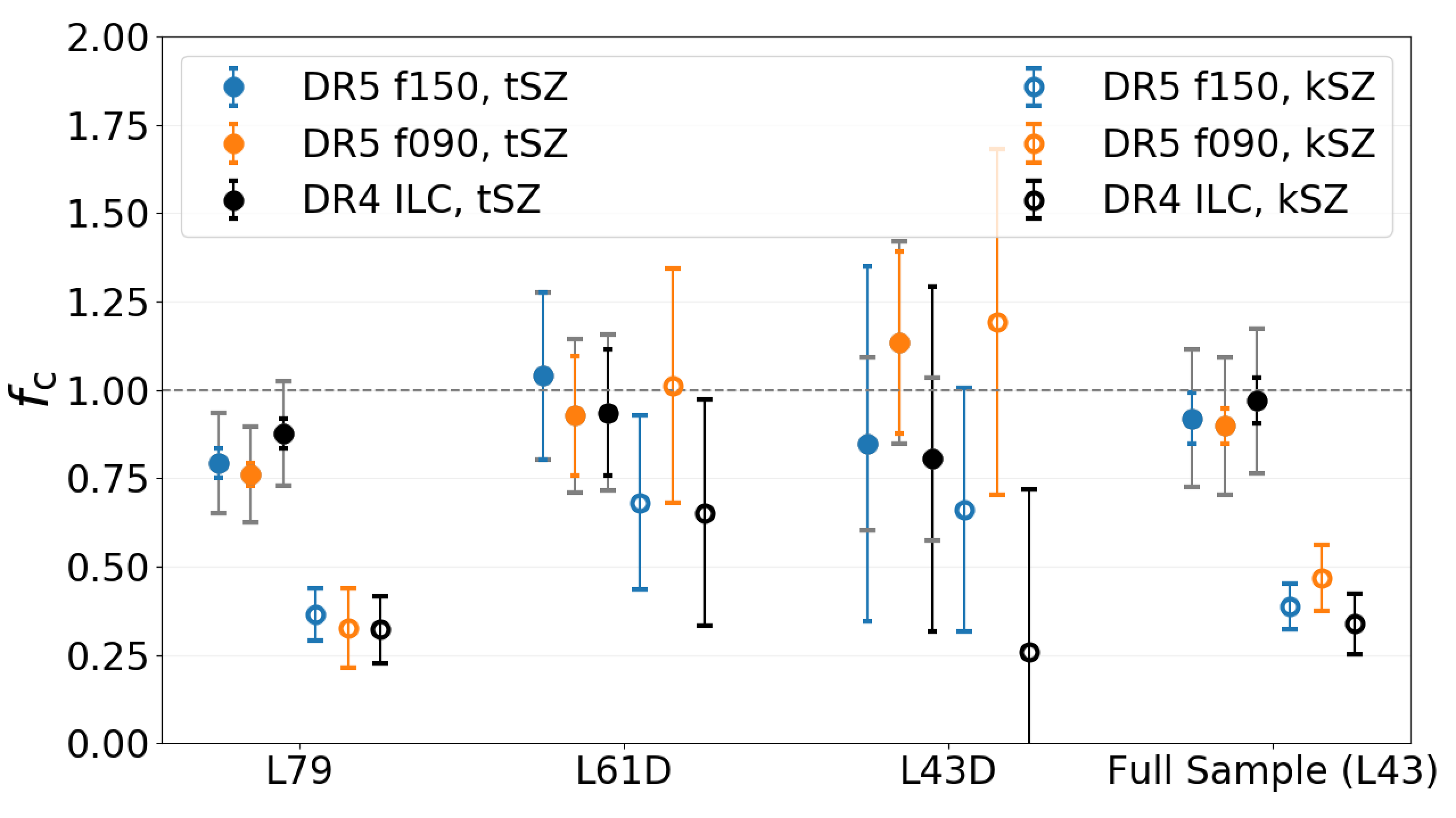
Figure 7: Fraction of the theoretically predicted optical depth ($f_{\rm c}$) for the full DR15 sample. The estimates are extracted from tSZ measurements (filled circles) from three different maps (DR5 f150: blue, DR5 f090: orange, and ILC: black) and kSZ measurements from the same maps, as described in C21 (open circles). The tSZ measurements are converted to optical depth estimates using a scaling relationship from hydrodynamic simulations Battaglia (2016). The tSZ jackknife uncertainties are plotted in color, and the systematic uncertainties from the simulation-based scaling relationship are plotted as grey bars. The plotted kSZ uncertainties are from bootstrap estimates. The kSZ and tSZ results agree within 1$\sigma$ in the L61D and L43D bins, while in the highest signal-to-noise L79 bin they differ at 2-3$\sigma$. This results in the 2-3$\sigma$ difference observed in the full sample, L43. The difference between the kSZ and tSZ results is discussed in Section IV.C. The kSZ results are lowest for the L79 bin.

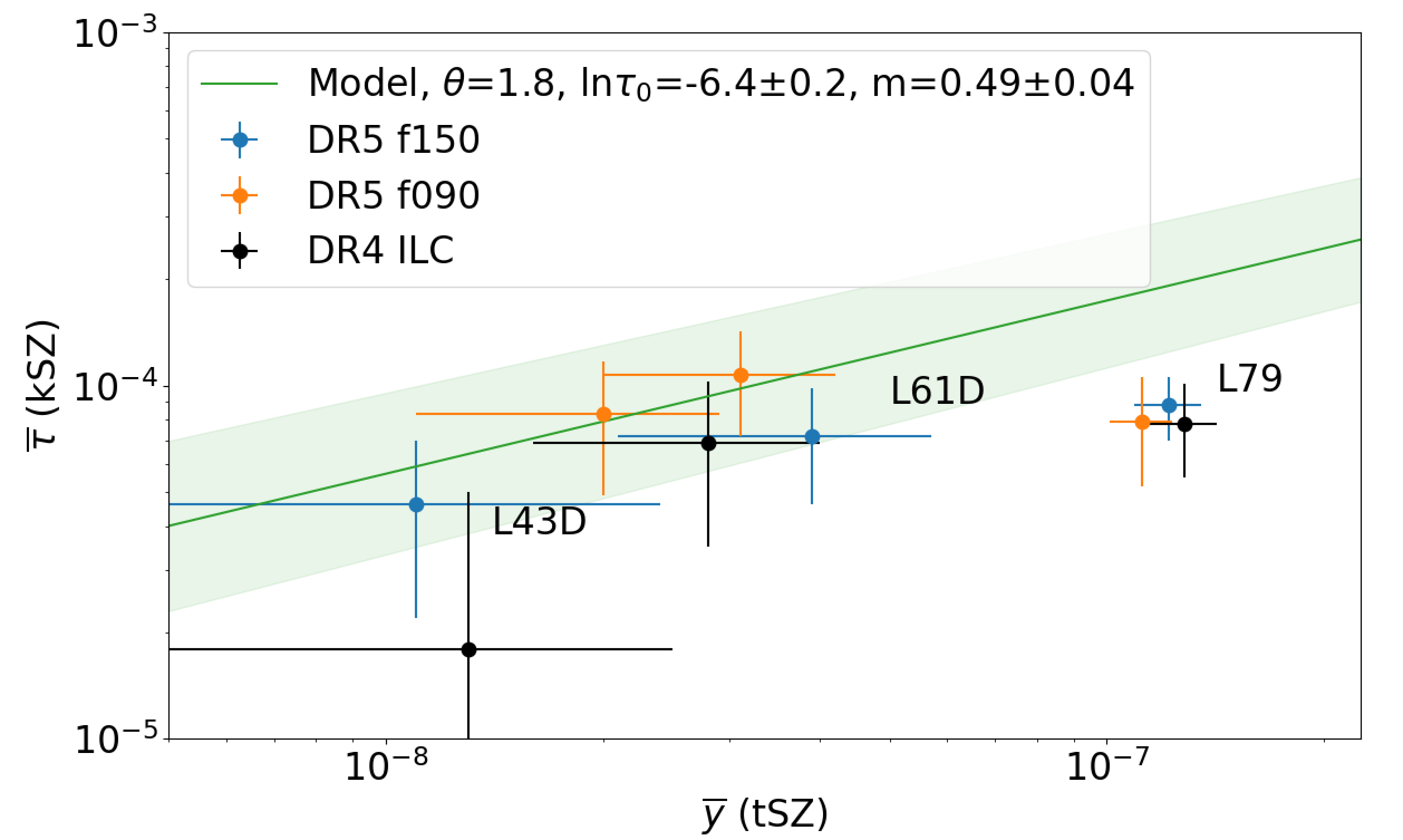
Figure 8: Optical depth fits from kSZ signals versus average Compton-$y$ from the tSZ measurements for the three jointly analyzed disjoint luminosity bins with statistical error bars from jackknife estimates (bootstrap estimated uncertainties for the kSZ, see C21). The scaling relation between $\bar{\tau}$ and $\bar{y}$ from hydrodynamical simulations with aperture $\Theta=1.8^{\prime}$ (the closest scaling relation in Battaglia (2016) to our $2.1^{\prime}$ aperture) is plotted as the green model curve (Equation 3) with the 1$\sigma$ uncertainty envelope shaded. The tSZ and kSZ results in the L43D and L61D luminosity bins are consistent with the model, while the kSZ results in the L79 bin fall below the model line.

IV Results

IV.A tSZ measurements

Table III presents values of $\delta T_{\rm tSZ}$ for each luminosity bin along with the averaged Compton $\bar{y}$ parameter we calculated using the tSZ signal. These results are beam and dust corrected using our Herschel-based estimates, and assume one source per filter (Section III.C). The signal-to-noise ratios for the tSZ measurements are up to 10 for the DR5 f150 map, 12 for the DR5 f090 map, and 10 for the ILC map, with the highest signal-to-noise in the L98 bin for the coadded maps, and the L116 bin for the ILC map. Before the Herschel dust corrections were applied and the uncertainties from those corrections propagated into the statistical tSZ uncertainty estimates, the highest signal-to-noise was seen in the highest luminosity bin (L116) for the coadded maps as well, which is as expected. The average Compton $\bar{y}$ from the tSZ signals in the three maps is presented in Figure 6 along with signal-to-noise per disjoint bin. The $\bar{y}$ measurements are consistent across the maps we analyzed.

The optical depths calculated using Eqn. 3 range from 0.59$\pm 0.35(\mathrm{stat.})\pm 0.17(\mathrm{sys.})\times 10^{-4}$ to 3.22$\pm 0.15(\mathrm{stat.})\pm 0.42(\mathrm{sys.})\times 10^{-4}$ for all nine luminosity bins and three maps, as reported in Table IV. Potential tSZ systematic effects are discussed in Section III.C.

IV.B kSZ measurements

C21 presented a value of $\bar{\tau}=(0.69\pm 0.11)\times 10^{-4}$ as the highest signal-to-noise best fit average optical depth. It was derived from the mean pairwise momentum for the full sample of 343,647 sources and DR5 f150 map using bootstrap uncertainty estimates of the pairwise correlation covariance matrix. In C21, we find that the analytical signal model is a good fit to the data with a best fit $\chi^{2}$ of 10 for 17 degrees of freedom. Selected best fit optical depths from the mean pairwise momentum fits and bootstrap estimated signal-to-noise are reported in Table IV, and shown in Figures 7 and 8, along with the results derived here.

IV.C Optical depth comparisons

Optical depth estimates from the two SZ effects are presented in Table IV along with comparisons to theory. Figure 7 presents the fraction of theoretically predicted optical depth ($f_{\rm c}$) for the three independent joint analysis bins and the full sample, a representation of the baryon fraction we observe within the AP radius for those source samples. The tSZ and kSZ estimates are consistent within $1\sigma$ for the two lower mass disjoint bins (L61D and L43D), while they differ at 2-3$\sigma$ in the highest mass bin (L79), which is also the best constrained. This difference drives 2-3$\sigma$ differences between the tSZ and kSZ results in the cumulative bins. This difference may be decreased if the fixed cosmology assumed for the kSZ optical depth fits were allowed to vary. We look forward to comparing the two tracers in more detail in future work with even more sensitive data sets. The addition of more disjoint bins with sufficient numbers of sources for high signal-to-noise kSZ measurements will aid in the interpretation of any mass-dependent effects. Additionally, the halo mass input in the kSZ theory fits in C21 will continue to be investigated in future analyses. The comparisons with theoretical estimates of the optical depth suggest that between one third and all of the predicted baryons lie within the aperture size of radius 2.1^′, or 1.1 Mpc (for a mean redshift of z = 0.55) studied in this analysis. However, because uncertainties in the luminosity-mass relation for DR15 (Section III.E) are difficult to accurately propagate through to $\bar{\tau}_{\mathrm{theory}}$, it is challenging to draw strong conclusions about baryon content based on our estimates of $f_{\rm c}$. For future high signal-to-noise measurements, careful treatment of the uncertainties, discussed in Kravtsov et al. (2018), will be necessary for accurate interpretation of these SZ results. Here, the $f_{\rm c}$ values are used for making comparisons between the SZ estimates and studying trends.

Figure 8 shows a comparison of $\bar{\tau}$ estimates from kSZ measurements and average Compton-$y$ from tSZ measurements to the power-law scaling relation using an AGN feedback model simulation relation (Equation 3) Battaglia (2016). We expect significant covariance between the data from the different maps. Two of the three disjoint analysis bins are in agreement with the model, while the highest mass bin (L79) is an outlier. This appears to be driven by low kSZ $\bar{\tau}$ estimates for this bin (Fig. 7).

The two-halo contribution to our tSZ measurements, discussed in Sec. III.C, does not affect these results. Propagating our $\bar{y}$ corrections to $\bar{\tau}_{tSZ}$ and then to $f_{\mathrm{c,tSZ}}$ (filled circles in Fig. 8), we get lower tSZ fractions by a factor of 4% for the L43D bin and less for the other bins.

Our fits represent a step towards empirical $\bar{y}$-$\bar{\tau}$ relationships from a fit to kSZ and tSZ measurements. These measurements will thus serve as tests and checks for current and future cosmological simulations, and improve our understanding of galaxy formation and feedback models.

V Conclusion

We have presented estimates of halo optical depths from measurements of the tSZ effect made on the most recent multi-frequency ACT+Planck maps in combination with LRG tracers from the SDSS BOSS DR15 catalog. By combining them with the kSZ measurements presented in C21, we compare estimates of optical depths from the two SZ effects and make progress towards empirical $\bar{y}-\bar{\tau}$ relationships from the SZ effects. We have improved our approach compared to our previous work, DB17, by analyzing the CMB map with the same AP filter for both the kSZ and tSZ analysis, and removing contaminating dust emission by estimating the contribution from dusty star-forming galaxies using Herschel maps and a modified blackbody dust emission model.

The stacked tSZ signals were converted to an estimate of optical depth through a hydrodynamic simulation scaling model Battaglia (2016), while the pairwise kSZ signals were fit to theoretical predictions to find best fit optical depths (C21). The two methods are independent of one another, and each of the SZ results is consistent over the three maps analyzed (DR5 f150, DR5 f090, and DR4 ILC). The results from the tSZ and kSZ measurements agree with one another within 1$\sigma$ in the two lower mass disjoint bins, while they differ by 2-3$\sigma$ in the highest mass bin and thus the cumulative bin. Across all bins, the optical depth estimates from the SZ effects account for one third to all of the theoretically predicted baryon content. When comparing the tSZ $\bar{y}$ measurements and kSZ $\bar{\tau}$ results to the hydrodynamic model, two of the three bins analyzed are in agreement with the model.

Using tSZ data appears to be a promising approach for obtaining accurate estimates of galaxy group and cluster optical depths and eventually estimating the mean pairwise velocity from pairwise momentum measurements, once a better understanding of the relationship between $\bar{y}$ and $\bar{\tau}$ is achieved. Our results help to move us from an era of measurement alone to one of interpretation based on the consistency of previously inaccessible quantities.

With improved data from the complete ACT dataset Henderson et al. (2016) and current and upcoming projects such as CCAT-prime Stacey et al. (2018), the Simons Observatory Simons Observatory Collaboration (2019), DESI Levi et al. (2019), SPT-3G Benson and et al. (2014) and CMB-S4 Abazajian et al. (2015), we will achieve higher signal-to-noise measurements of the SZ signals and be able to probe the baryon content of galaxy clusters and groups and large-scale structure further. Improved multi-frequency data will enable precise measurements of optical depths and peculiar velocities simultaneously for large samples and for single sources, potentially sensitive enough to measure the missing baryons between groups. With these data, the SZ signals are anticipated to become valuable cosmological probes that are complementary to current observables.

VI Acknowledgements

EMV acknowledges support from the NSF Graduate Research Fellowship Program under Grant No. DGE-1650441. MDN acknowledges support from NSF CAREER award 1454881. VC and RB acknowledge support from DoE grant DE-SC0011838, NASA ATP grant 80NSSC18K0695, NASA ROSES grant 12-EUCLID12-0004 and funding related to the Roman High Latitude Survey Science Investigation Team. NB acknowledges support from NSF grant AST-1910021, NASA ATP grant 80NSSC18K0695 and from the Research and Technology Development fund at the Jet Propulsion Laboratory through the project entitled “Mapping the Baryonic Majority”. EC acknowledges support from the STFC Ernest Rutherford Fellowship ST/M004856/2 and STFC Consolidated Grant ST/S00033X/1, and from the European Research Council (ERC) under the European Union’s Horizon 2020 research and innovation programme (Grant agreement No. 849169). SKC acknowledges support from NSF award AST-2001866. JD is supported through NSF grant AST-1814971. RD thanks CONICYT for grant BASAL CATA AFB-170002. RH acknowledges funding from the CIFAR Azrieli Global Scholars program and the Alfred P. Sloan Foundation. JPH acknowledges funding for SZ cluster studies from NSF grant number AST-1615657. KM acknowledges support from the National Research Foundation of South Africa. CS acknowledges support from the Agencia Nacional de Investigación y Desarrollo (ANID) through FONDECYT Iniciación grant no. 11191125. ZX is supported by the Gordon and Betty Moore Foundation.

This work was supported by the U.S. National Science Foundation through awards AST-0408698, AST-0965625, and AST-1440226 for the ACT project, as well as awards PHY-0355328, PHY-0855887 and PHY-1214379. Funding was also provided by Princeton University, the University of Pennsylvania, and a Canada Foundation for Innovation (CFI) award to UBC. ACT operates in the Parque Astronómico Atacama in northern Chile under the auspices of the Comisión Nacional de Investigación Científica y Tecnológica de Chile (CONICYT).

Canadian co-authors acknowledge support from the Natural Sciences and Engineering Research Council of Canada. The Dunlap Institute is funded through an endowment established by the David Dunlap family and the University of Toronto.

Funding for the Sloan Digital Sky Survey IV has been provided by the Alfred P. Sloan Foundation, the U.S. Department of Energy Office of Science, and the Participating Institutions. SDSS-IV acknowledges support and resources from the Center for High Performance Computing at the University of Utah. The SDSS website is www.sdss.org. SDSS-IV is managed by the Astrophysical Research Consortium for the Participating Institutions of the SDSS Collaboration including the Brazilian Participation Group, the Carnegie Institution for Science, Carnegie Mellon University, Center for Astrophysics — Harvard & Smithsonian, the Chilean Participation Group, the French Participation Group, Instituto de Astrofísica de Canarias, The Johns Hopkins University, Kavli Institute for the Physics and Mathematics of the Universe (IPMU) / University of Tokyo, the Korean Participation Group, Lawrence Berkeley National Laboratory, Leibniz Institut für Astrophysik Potsdam (AIP), Max-Planck-Institut für Astronomie (MPIA Heidelberg), Max-Planck-Institut für Astrophysik (MPA Garching), Max-Planck-Institut für Extraterrestrische Physik (MPE), National Astronomical Observatories of China, New Mexico State University, New York University, University of Notre Dame, Observatário Nacional / MCTI, The Ohio State University, Pennsylvania State University, Shanghai Astronomical Observatory, United Kingdom Participation Group, Universidad Nacional Autónoma de México, University of Arizona, University of Colorado Boulder, University of Oxford, University of Portsmouth, University of Utah, University of Virginia, University of Washington, University of Wisconsin, Vanderbilt University, and Yale University.

Appendix A CasJobs SDSS Query

The SDSS data used in this work and C21 was downloaded from the SDSS Catalog Archive Server (CAS) via the SkyServer website in May of 2019. All of the CMASS and LOWZ galaxies should be included in this catalog, in addition to more recently released eBOSS galaxies. We use this approach in defining the catalog to utilize as many SDSS LRGs as possible. The following query returned 602,461 objects. The positions, redshifts, cmodel and Petrosian magnitudes, extinction corrections, and object IDs are recorded for the objects. An RA and DEC cut is applied to target the survey area overlapping with our maps, and the redshifts of the objects are selected to match the range in DB17. “ZWARNING$\_$NOQSO=0” indicates that the automated redshift estimate is reliable for the source. Objects with “zWarning=0” have no known redshift issues. Querying with “sciencePrimary$>$0” selects the best available unique set of spectra for the objects. Bitmasks are applied to exclude SDSS target flags: “SpecObjAll.TILE$>=$ 10324” excludes incorrectly targeted LOWZ galaxies in early BOSS data, and the i-band fiber magnitude is selected to be the same as in DB17.

⬇

SELECT

SpecObjAll.ra, SpecObjAll.dec, SpecObjAll.z,

PhotoObjAll.cModelMag_u,PhotoObjAll.cModelMag_g,PhotoObjAll.cModelMag_r,PhotoObjAll.cModelMag_i,PhotoObjAll.cModelMag_z,PhotoObjAll.cModelMagErr_u,PhotoObjAll.cModelMagErr_g,

PhotoObjAll.cModelMagErr_r,PhotoObjAll.cModelMagErr_i,PhotoObjAll.cModelMagErr_z,

PhotoObjAll.petroMag_u,PhotoObjAll.petroMag_g,PhotoObjAll.petroMag_r,PhotoObjAll.petroMag_i,PhotoObjAll.petroMag_z,PhotoObjAll.petroMagErr_u,PhotoObjAll.petroMagErr_g,

PhotoObjAll.petroMagErr_r,PhotoObjAll.petroMagErr_i,PhotoObjAll.petroMagErr_z,PhotoObjAll.extinction_u,PhotoObjAll.extinction_g,PhotoObjAll.extinction_r,PhotoObjAll.extinction_i,

PhotoObjAll.extinction_z,SpecObjAll.bestObjID into DR15_actplanck_catalog_wbestObjID_PetrANDcModel_20200902_EMV from SpecObjAll, PhotoObjAll, Photoz

WHERE

((SpecObjAll.bestObjID = PhotoObjAll.objID) and (SpecObjAll.bestObjID = Photoz.objID))

and

((((SpecObjAll.ra BETWEEN 142.0 AND 180.0) and (SpecObjAll.dec BETWEEN -8.3 AND 22.0)) or ((SpecObjAll.ra BETWEEN 0.0 AND 142.0) and (SpecObjAll.dec BETWEEN -61.5 AND 22.0))

or ((SpecObjAll.ra BETWEEN 246.0 AND 360.0) and (SpecObjAll.dec BETWEEN -61.5 AND 22.0)) or ((SpecObjAll.ra BETWEEN 180.0 AND 246.0) and (SpecObjAll.dec BETWEEN -8.3 AND 22.0)))

and (SpecObjAll.ZWARNING_NOQSO = 0) and

(SpecObjAll.zWarning = 0) AND

(SpecObjAll.sciencePrimary>0) and

(SpecObjAll.z>0.049) and

(SpecObjAll.z<0.8) and

((((SpecObjAll.BOSS_TARGET1 & 0x0000000000000001) != 0) and

(SpecObjAll.TILE>= 10324)) OR

(((SpecObjAll.BOSS_TARGET1 & 0x0000000000000002)!=0) and

(PhotoObjAll.fiber2Mag_i<21.5))))

Appendix B Luminosity Binning

As discussed in Section II.B, luminosity bins for the joint tSZ and kSZ analyses with C21 were chosen based on luminosity cuts from DB17 ($L>7.9\times 10^{10}L_{\odot}$ and $L>6.1\times 10^{10}L_{\odot}$) as well as one lower luminosity cut, ($L>4.3\times 10^{10}L_{\odot}$). The three disjoint bins were selected to have roughly equal spacing, each with $\sim$100,000 galaxies after cutting for analysis with the DR5 maps (Table I). The luminosity cuts are plotted over a histogram of the SDSS samples in Figure 9.

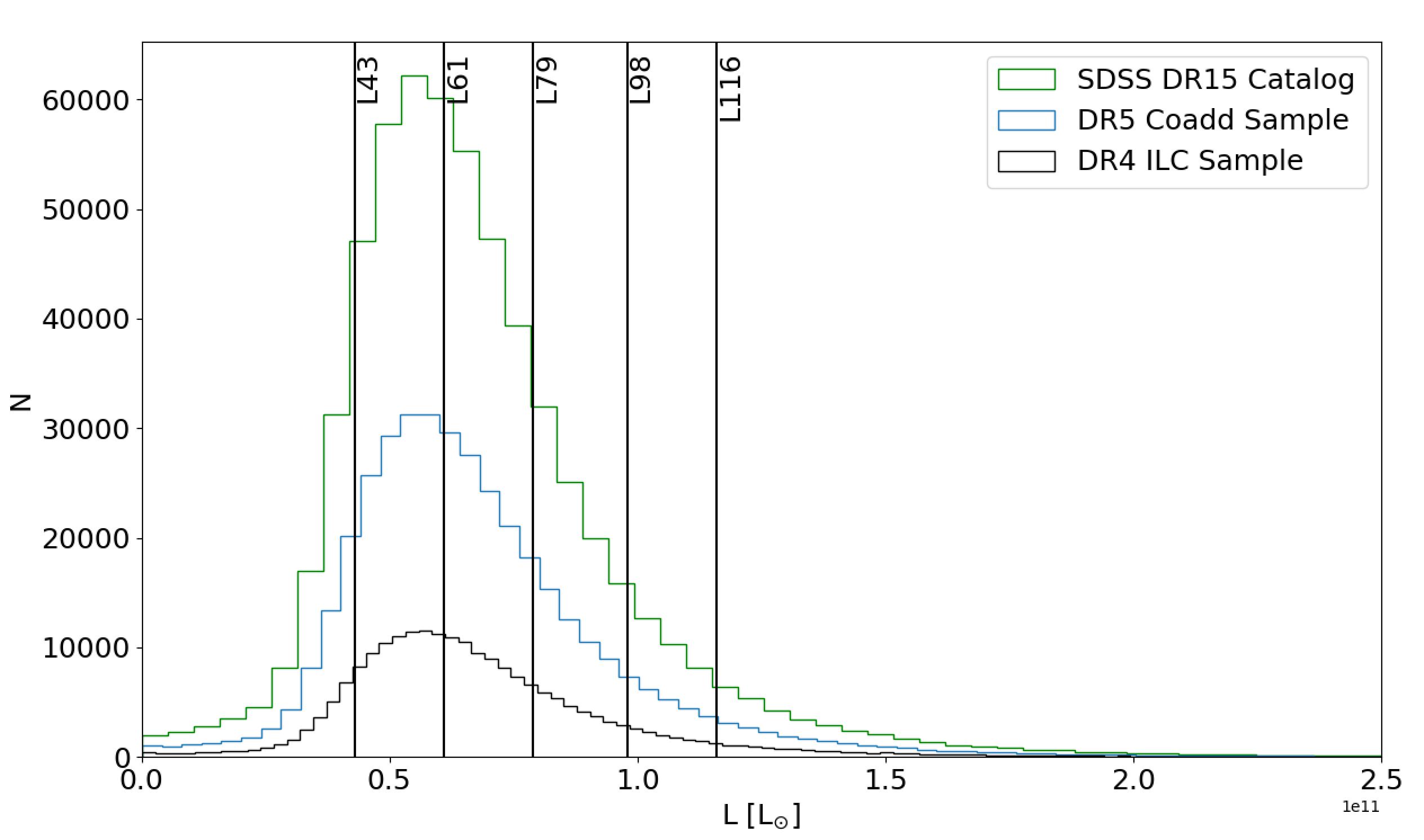
Figure 9: Luminosity bin cuts for the SDSS DR15 catalog plotted over a histogram of the full sample (green), DR5 f150 and DR5 f090 selected analysis sample (blue), and DR4 ILC sample (black). The bottom three bins were selected to each have over 100,000 galaxies for the joint tSZ and kSZ analyses of the DR5 maps, while being roughly evenly spaced and overlapping with bin selection from the DB17 analysis. The top two bins were added for the tSZ analysis to study higher mass bins that have a strong tSZ signal, while also overlapping with DB17 bins.

References

- Zeldovich and Sunyaev (1969) Y. B. Zeldovich and R. A. Sunyaev, Ap&SS 4, 301 (1969).
- Sunyaev and Zeldovich (1972) R. A. Sunyaev and Y. B. Zeldovich, Comments on Astrophysics and Space Physics 4, 173 (1972).
- Battaglia (2016) N. Battaglia, JCAP 8, 058 (2016), eprint arXiv:1607.02442.
- Mroczkowski et al. (2019) T. Mroczkowski et al., BAAS 51, 124 (2019), eprint arXiv:1903.02595.
- Fukugita and Peebles (2004) M. Fukugita and P. J. E. Peebles, ApJ 616, 643 (2004), eprint astro-ph/0406095.
- Nicastro et al. (2008) F. Nicastro, S. Mathur, and M. Elvis, Science (New York, N.Y.) 319, 55 (2008), ISSN 0036-8075, URL http://www.sciencemag.org/cgi/content/full/319/5859/55.
- Shull et al. (2012) J. M. Shull, B. D. Smith, and C. W. Danforth, ApJ 759, 23 (2012), eprint arXiv:1112.2706.
- Rasheed et al. (2011) B. Rasheed, N. Bahcall, and P. Bode, Proceedings of the National Academy of Sciences 108, 3487 (2011), ISSN 0027-8424.
- Chiu et al. (2018) I. Chiu, J. J. Mohr, M. McDonald, S. Bocquet, et al., Monthly Notices of the Royal Astronomical Society 478, 3072–3099 (2018), ISSN 1365-2966.
- Schaan et al. (2016) E. Schaan et al., Phys. Rev. D 93, 082002 (2016).
- Ho et al. (2009) S. Ho, S. DeDeo, and D. Spergel (2009), eprint arXiv:0903.2845.
- Richter et al. (2005) P. Richter, B. D. Savage, T. M. Tripp, and K. R. Sembach, IAU Colloq. 199: Probing Galaxies through Quasar Absorption Lines pp. 469–471 (2005), eprint astro-ph/0412133.
- Cen and Ostriker (2006) R. Cen and J. P. Ostriker, ApJ 650, 560 (2006), eprint astro-ph/0601008.
- Chaves-Montero et al. (2019) J. Chaves-Montero, C. Hernandez-Monteagudo, R. E. Angulo, and J. D. Emberson, arXiv e-prints 1911.10690 (2019).
- Hand et al. (2012) N. Hand et al. (ACT), Phys. Rev. Lett. 109, 041101 (2012), eprint arXiv:1203.4219.
- Mueller et al. (2015) E.-M. Mueller, F. de Bernardis, R. Bean, and M. D. Niemack, Phys. Rev. D 92, 063501 (2015), eprint arXiv:1412.0592.
- Mueller et al. (2015) E.-M. Mueller, F. de Bernardis, R. Bean, and M. D. Niemack, ApJ 808, 47 (2015), eprint arXiv:1408.6248.
- Marriage et al. (2011) T. A. Marriage et al. (ACT), ApJ 737, 61 (2011), eprint arXiv:1010.1065.
- Hasselfield et al. (2013) M. Hasselfield et al. (ACT), JCAP 1307, 008 (2013), eprint arXiv:1301.0816.
- Hilton et al. (2018) M. Hilton, M. Hasselfield, C. Sifón, N. Battaglia, et al. (ACT), ApJS (2018), eprint arXiv:1709.05600.
- Aghanim et al. (2019) N. Aghanim, M. Douspis, G. Hurier, D. Crichton, et al., A&A 632, A47 (2019), eprint arXiv:1902.00350.
- Staniszewski et al. (2009) Z. Staniszewski et al., ApJ 701, 32 (2009), eprint arXiv:0810.1578.
- Bleem et al. (2015) L. Bleem, B. Stalder, T. de Haan, et al., ApJS 216, 27 (2015), eprint arXiv:1409.0850.
- Planck Collaboration (2020) Planck Collaboration, A&A 641, A1 (2020), eprint arXiv:1807.06205.
- Fuzia et al. (2020) B. J. Fuzia et al. (ACT) (2020), eprint arXiv:2001.09587.
- Gralla et al. (2014) M. B. Gralla et al., MNRAS 445, 460 (2014), eprint arXiv:1310.8281.
- Su et al. (2017) T. Su et al., MNRAS 464, 968 (2017), eprint arXiv:1511.06770.
- Naess et al. (2020) S. Naess et al. (ACT) (2020), eprint arXiv:2007.07290.
- Madhavacheril et al. (2020) M. S. Madhavacheril, J. C. Hill, S. Næss, et al. (ACT), Phys. Rev. D 102, 023534 (2020), eprint arXiv:1911.05717.
- Aguado et al. (2019) D. S. Aguado et al., ApJS 240, 23 (2019), eprint arXiv:1812.02759.
- Planck Collaboration (2016a) Planck Collaboration, A&A 594, A22 (2016a), eprint arXiv:1502.01596.
- Calafut et al. (2021) V. Calafut, P. A. Gallardo, E. M. Vavagiakis, S. Amodeo, et al. (ACT) (2021), eprint arXiv:2101.08374.
- De Bernardis et al. (2017) F. De Bernardis et al. (ACT), JCAP 1703, 008 (2017), eprint arXiv:1607.02139.
- Ferreira et al. (1999) P. G. Ferreira, R. Juszkiewicz, H. A. Feldman, et al., ApJ 515, L1 (1999), eprint astro-ph/9812456.
- Planck Collaboration (2016b) Planck Collaboration, A&A 586, A140 (2016b), eprint arXiv:1504.03339.
- Soergel et al. (2016) B. Soergel et al., MNRAS 461, 3172 (2016), eprint arXiv:1603.03904.
- Hand et al. (2011) N. Hand et al., ApJ 736, 39 (2011), eprint arXiv:1101.1951.
- Amodeo et al. (2020) S. Amodeo et al. (ACT) (2020), eprint arXiv:2009.05558.
- Schaan et al. (2020) E. Schaan et al. (ACT) (2020), eprint arXiv:2009.05557.
- Ahn et al. (2014) C. P. Ahn et al., ApJS 211, 17 (2014), eprint arXiv:1307.7735.
- Thornton et al. (2016) R. J. Thornton et al. (ACT), ApJS 227, 21 (2016), eprint arXiv:1605.06569.
- Dawson et al. (2013) K. S. Dawson et al., Astron. J. 145, 10 (2013), eprint arXiv:1208.0022.
- Calafut et al. (2017) V. Calafut, R. Bean, and B. Yu, Phys. Rev. D 96, 123529 (2017), eprint arXiv:1710.01755.
- Blanton and Roweis (2007) M. R. Blanton and S. Roweis, AJ 133, 734 (2007), eprint astro-ph/0606170.
- Lupton et al. (1999) R. H. Lupton, J. E. Gunn, and A. S. Szalay, AJ 118, 1406 (1999), eprint astro-ph/9903081.
- Choi et al. (2020) S. K. Choi et al. (ACT) (2020), eprint arXiv:2007.07289.
- Chabrier (2003) G. Chabrier, PASP 115, 763 (2003), eprint astro-ph/0304382.
- Kravtsov et al. (2018) A. Kravtsov, A. Vikhlinin, and A. Meshcheryakov, Astron. Lett. 44, 8 (2018).
- Bell and de Jong (2001) E. F. Bell and R. S. de Jong, ApJ 550, 212 (2001), eprint astro-ph/0011493.
- Bell et al. (2003) E. F. Bell, D. H. McIntosh, N. Katz, and M. D. Weinberg, ApJS 149, 289 (2003), eprint astro-ph/0302543.
- Bernardi et al. (2010) M. Bernardi, F. Shankar, J. B. Hyde, S. Mei, F. Marulli, and R. K. Sheth, MNRAS 404, 2087 (2010), eprint arXiv:0910.1093.
- Battaglia et al. (2012) N. Battaglia, J. R. Bond, C. Pfrommer, and J. L. Sievers, ApJ 758, 75 (2012), eprint arXiv:1109.3711.
- Itoh et al. (2000) N. Itoh, S. Nozawa, and Y. Kohyama, ApJ 533, 588 (2000), eprint astro-ph/9812376.
- Hilton et al. (2020) M. Hilton et al. (ACT), arXiv:2009.11043 (2020).
- Nozawa et al. (2006) S. Nozawa, N. Itoh, Y. Suda, and Y. Ohhata, Nuovo Cimento B Serie 121, 487 (2006), eprint astro-ph/0507466.
- Eales et al. (2010) S. Eales et al., PASP 122, 499 (2010), eprint arXiv:0910.4279.
- Foreman-Mackey et al. (2013) D. Foreman-Mackey, D. W. Hogg, D. Lang, and J. Goodman, PASP 125, 306 (2013), eprint arXiv:1202.3665.
- Hill et al. (2018) J. C. Hill, E. J. Baxter, A. Lidz, J. P. Greco, and B. Jain, Phys. Rev. D 97, 083501 (2018), eprint arXiv:1706.03753.
- Hamilton et al. (1991) A. J. S. Hamilton, P. Kumar, E. Lu, and A. Matthews, ApJ 374, L1 (1991).
- Nityananda and Padmanabhan (1994) R. Nityananda and T. Padmanabhan, Mon. Not. Roy. Astron. Soc. 271, 976 (1994), eprint gr-qc/9304022.
- Juszkiewicz et al. (1999) R. Juszkiewicz, V. Springel, and R. Durrer, ApJ 518, L25 (1999), eprint astro-ph/9812387.
- Sheth et al. (2001) R. K. Sheth, A. Diaferio, L. Hui, and R. Scoccimarro, Mon. Not. Roy. Astron. Soc. 326, 463 (2001), eprint astro-ph/0010137.
- Bhattacharya and Kosowsky (2008) S. Bhattacharya and A. Kosowsky, Phys. Rev. D 77, 083004 (2008), eprint arXiv:0712.0034.
- Henderson et al. (2016) S. W. Henderson et al., Journal of Low Temperature Physics 184, 772 (2016), eprint arXiv:1510.02809.
- Stacey et al. (2018) G. J. Stacey et al., Proc. SPIE Ground-based and Airborne Telescopes VII 10700, 107001M (2018), eprint arXiv:1807.04354.
- Simons Observatory Collaboration (2019) Simons Observatory Collaboration, J. Cosmology Astropart. Phys 2019, 056 (2019), eprint arXiv:1808.07445.
- Levi et al. (2019) M. Levi et al., Bulletin of the American Astronomical Society 51, 57 (2019), eprint arXiv:1907.10688.
- Benson and et al. (2014) B. A. Benson and et al., Proc. SPIE Millimeter, Submillimeter, and Far-Infrared Detectors and Instrumentation for Astronomy VII 9153, 91531P (2014), eprint arXiv:1407.2973.
- Abazajian et al. (2015) K. N. Abazajian et al., Astropart. Phys. 63, 66 (2015), eprint arXiv:1309.5383.