Uniqueness of excited states to $-\Delta u+u-u^{3}=0$ in three dimensions

Abstract.

We prove the uniqueness of several excited states to the ODE $\ddot{y}(t)+\frac{2}{t}\dot{y}(t)+f(y(t))=0$, $y(0)=b$, and $\dot{y}(0)=0$ for the model nonlinearity $f(y)=y^{3}-y$. The $n$-th excited state is a solution with exactly $n$ zeros and which tends to $0$ as $t\to\infty$. These represent all smooth radial nonzero solutions to the PDE $\Delta u+f(u)=0$ in $H^{1}$. We interpret the ODE as a damped oscillator governed by a double-well potential, and the result is proved via rigorous numerical analysis of the energy and variation of the solutions. More specifically, the problem of uniqueness can be formulated entirely in terms of inequalities on the solutions and their variation, and these inequalities can be verified numerically.

1. Introduction

Consider the ODE

$$\ddot{y}(t)+\frac{2}{t}\dot{y}(t)+f(y(t))=0,$$ (1.1)

$$y(0)=b,\ \dot{y}(0)=0.$$ (1.2)

In this paper, we will only consider the model case $f(y)=y^{3}-y$, but it will be convenient to use the more general notation for the nonlinearity. Smooth solutions to this ODE exist for all $t\geq 0$ and any $b\in\mathbb{R}$, and they are unique. We denote them by $y_{b}$, or simply $y$. The singular coefficient at $t=0$ can be dealt with by a power series ansatz, or by Picard iteration. Solutions to this ODE correspond to radial smooth solutions of the PDE

$$\begin{split}\Delta u+f(u)=0\end{split}$$ (1.3)

in three dimensions, under the identification $t=r$, the radial variable. Dynamics of (1.1) resembles particle motion in a double well as in Figure 1, with time varying friction.

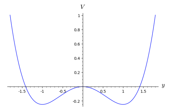
Figure 1. Potential function $V(y)$

The qualitative behavior exhibits a trichotomy: we either have

• $(y_{b}(t),\dot{y}_{b}(t))\to(1,0)$

• $(y_{b}(t),\dot{y}_{b}(t))\to(-1,0)$

• $(y_{b}(t),\dot{y}_{b}(t))\to(0,0)$,

see Section 3 below. A bound state is a nonzero solution with $y(t)\to 0$. Only these solutions give rise to nontrivial solutions $u\in H^{1}(\mathbb{R}^{3})$ of the elliptic PDE (1.3). A ground state is a positive bound state, and an $n^{th}$ excited state is a bound state with precisely $n$ zero crossings. The $0^{th}$ bound state is the ground state. Existence and uniqueness of these bound states have been investigated since the 1960s. In 1967, using a variational characterization, Ryder [20, Theorem II] showed the existence of both ground and excited states with any finite number of zero crossings. In 1972, Coffman [6, Section 6] related Ryder’s characteristic values to degree theory in infinite dimensions and Lyusternik-Schnirelman techniques. Most importantly, [6] also established uniqueness of the ground state for the cubic case. For more general nonlinearities, ground state uniqueness was then shown by Peletier, Serrin [19, 18], McLeod, Serrin [13], Zhang [24], Kwong [11], and finally in greatest generality by McLeod in 1992 [12]. Clemons, Jones [5] gave a different proof of McLeod’s theorem based on the Emden-Folwer transformation and unstable manifold theory. In 1983, Berestycki and Lions [1, 2] solved the existence problem of radial bound states for (1.3) for all $H^{1}$ subcritical nonlinearities $f(u)$ in all dimensions, see also the earlier work by Strauss [21].

However, uniqueness of exited states in the radial class, i.e., for the ODE (1.1), remained open for most nonlinearities. In fact, in their 2012 text, Hastings, McLeod [10, Chapter 19] list this problem as one of three major open problems in nonlinear ODEs. We note that there has been some uniqueness results for specific nonlinearities; in 2005, Troy [23] proved the uniqueness of the first excited state for a piecewise linear nonlinearity by analyzing the explicit solutions, and in 2009, Cortázar, García-Huidobro, and Yarur [7] proved uniqueness of the first excited state with restrictions on $yf^{\prime}(y)/f(y)$. However, neither cover the cubic nonlinearity. In this paper, we provide a rigorous computer-assisted proof of the uniqueness of the first excited state for the cubic nonlinearity. The proof technique combines analytical dynamics with the rigorous ODE solver VNODE-LP, see Section 2.3 and [16]. The latter works with interval arithmetic and therefore does not compute precise solutions (which is impossible), but rather intervals containing the solution at any given time. These inclusions accommodate all errors incurred through floating point arithmetic, and are therefore themselves free of errors.

Theorem 1.

The first twenty excited states of ODE (1.1-1.2) are unique for $f(y)=-y+y^{3}$.

The method is robust, and extends to both more general nonlinearities, as well as other dimensions. But we will leave the verification of this claim for another paper. The code involved in the proof is publicly available, see the GitHub repository https://github.com/alexander-cohen/NLKG-Uniqueness-Prover. The readers can verify uniqueness of higher excited states beyond the $20^{th}$ using the arguments of this paper. Computation time is the main obstacle to going further than the twentieth one, to which the authors chose to limit themselves. See Figure 2 for a graph of the limiting position of $y_{b}(T)$ as a function of $b$, up to the twentieth excited state. The rigorous numerical work done in this paper proves that this graph holds.

The uniqueness property of the ground state soliton is of fundamental importance to the classification of its long-term evolution under the nonlinear cubic Schrödinger or Klein-Gordon flows. See for example [4] and [14]. The uniqueness property of the excited states should therefore also be seen as a bridge to dynamical results. As a first step, one needs to determine the spectrum of the linearized operator

$$H=-\Delta+1-3\phi^{2}$$

in the radial subspace of $L^{2}(\mathbb{R}^{3})$. Here $\phi$ is any radial bound state solution of the PDE (1.3). If $\phi$ is the ground state, then it is known that the spectrum over the radial functions contains a unique negative eigenvalue, and no other discrete spectrum up to and including $0$ energy (nonradially, due to the translation symmetry, $0$ is an eigenvalue of multiplicity $3$); see [14]. A particularly delicate question pertains to the shape of the spectrum in the interval $(0,1]$, including the threshold $1$ of the (absolutely) continuous spectrum. This was settled in [8] for the ground state of the cubic power in three dimensions. It turns out that $(0,1]$ is a spectral gap, including the threshold, which is not a resonance. Due to the absence of an explicit expression of the ground state soliton, the method of [8] depended on an approximation of this special solution. Note that without uniqueness such an approximation has no meaning. The authors intend to investigate the spectral problem of excited states in another publication using the methods of [9], which essentially require the uniqueness property of the special solution $\phi$ (in the case of [9] $\phi$ is the so-called Skyrmion).

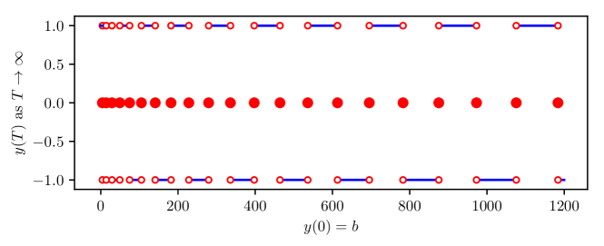
Figure 2. Limiting position $y_{b}(T)$ as $T\to\infty$, plotted as a function of $b$ up to the 20th excited state. This graph holds due to Theorem 1 and the rigorous numerical work done in this paper.

2. Overview of approach

2.1. Toy example: finding zeros of a function

Suppose we wish to find the number of zeros of the function $f$ as shown in the figure. Numerical computations make it clear that $f$ has exactly 3 zeros – how can we use a computer to prove this rigorously?

A first approach might be to find the approximate location of those zeros with reasonably high precision, using floating point arithmetic. Say they lie at approximately $y_{1},y_{2},y_{3}$. Then we can use interval arithmetic to show rigorously that $f$ is bounded away from zero everywhere but the three small intervals $(y_{1}-1/100,y_{1}+1/100)$, $(y_{2}-1/100,y_{2}+1/100)$, $(y_{3}-1/100,y_{3}+1/100)$. Then, by interval arithmetic combined with the intermediate value theorem, $f$ has at least one zero in each of these intervals. Finally, to show that each of them contains at most one zero, we can apply the mean value theorem. If we prove rigorously, using interval arithmetic, that $f^{\prime}$ is bounded away from zero in those intervals, then uniqueness follows.

Notice that if $f$ has infinitely many zeros with a limit point, then $f^{\prime}$ must be zero at that limit point. As expected, this method would break down in such a scenario.

2.2. Finding and isolating excited states

We apply a similar idea to the ODE (1.1). We now outline the approach by means of the ground state. Suppose we find numerically that the unique ground state should be at height $b_{0}\approx 4.3373$. Using a rigorous ODE solver, we can prove that for all $b\in(1,b_{0}-0.001)$, $y_{b}(t)>0$ up to some time $T$, and $E(T)<0$. This will imply by analytical arguments, see the next section, that $y_{b}(t)\to 1$ and $y_{b}(t)$ is positive, so it is not a ground state. Similarly, we can show that for $b\in(b_{0}+0.001,50)$, the solution passes over $y=0$, and thus is not a ground state. It follows from a connectedness argument that there is some ground state in the interval $(b_{0}-0.001,b_{0}+0.001)$. To prove that there is exactly one ground state in that interval, we find some large time $T$ such that $\delta_{b}(T),\dot{\delta}_{b}(T)<0$ for all $b\in(b_{0}-0.001,b_{0}+0.001)$, where $\delta_{b}=\partial_{b}y_{b}$. This means that if $b_{0}^{*}$ is the actual ground state (rather than an approximation), for any $b>b_{0}^{*}$ in our interval, $y_{b}(T)<y_{b_{0}^{*}}(T)$ and $\dot{y}_{b}(T)<\dot{y}_{b_{0}^{*}}(T)$ by the mean value theorem. One can then prove assuming this condition that $y_{b}(T)$ crosses over zero and lands in the second well, see Lemma 7. This will show that there is at most one ground state in the interval $(b_{0}-0.001,b_{0}+0.001)$. All that remains is showing that there is no ground state in the range $(50,\infty)$. To this end, we rescale the ODE (1.1) so that it takes the form $\ddot{w}+\frac{2}{t}\dot{w}+w^{3}-b^{-2}w=0$, $w(0)=1$, $\dot{w}(0)=0$. Again using VNODE-LP we then show that the solution of this equation exhibits more than any given number of zeros provided $b$ is sufficiently large. This then implies the same for $y_{b}$.

The same approach works just as well for excited states as it does for ground states.

2.3. Approximating solutions via interval arithmetic

We now outline our computational approach. Our main tool is the VNODE-LP package for rigorous ODE solving. The supporting website is at [15], and the documentation is available at [17].

VNODE-LP uses exact interval arithmetic, a toolset which allows for rigorous numerical computations. Rather than computing with floating point numbers as usual, interval arithmetic treats all values as intervals of real numbers, of the form $\mathbf{a}=[a_{1},a_{2}]$ where $a_{1},a_{2}$ are machine representable floating point numbers. All mathematical operations are rounded properly so that any input within the original interval ends up within the output interval. The VNODE-LP package combines interval arithmetic with ODE solving: given an initial value problem $\dot{y}=f(y,t)$ with initial values in an interval $\mathbf{b}$, a starting time interval $\mathbf{t}_{1}$, and an ending time interval $\mathbf{t}_{2}$, the package outputs an interval $\mathbf{y}$ such that for any $b\in\mathbf{b}$, $t_{1}\in\mathbf{t}_{1}$, $t_{2}\in\mathbf{t}_{2}$, $y_{b,t_{1}}(t_{2})\in\mathbf{y}$.

A difficulty in applying VNODE-LP to our problem is that ODE (1.1) is singular at $t=0$. To deal with this, we approximate $y_{b}(t)$ near $t=0$ by Picard iteration. We explicitly bound the error terms in this approximation so that we can rigorously obtain an interval containing $y_{b}(t_{0}),\dot{y}_{b}(t_{0})$ for $t_{0}$ small. Then VNODE-LP can be applied to this desingularized initial value problem, and all in all we we will have rigorous bounds on our solutions and quantities defined in terms of the solutions.

Section 5 explains in detail how we use this software, and provides links to websites containing the code and all supporting data needed in the proof of our theorem. This will hopefully allow the reader to implement the methods of this paper in other related settings.

3. Analytical description of the damped oscillator dynamics

3.1. Basic properties of the ODE

It is an elementary property that smooth solutions of (1.1), (1.2) exist for all times $t\geq 0$; in fact, we will reestablish this fact below in passing. Taking it for granted, we note that the energy

$$E(t):=\frac{1}{2}\dot{y}^{2}(t)+V(y(t))=\frac{1}{2}\dot{y}^{2}(t)+\frac{1}{4}y(t)^{4}-\frac{1}{2}y(t)^{2}$$

satisfies

$$\dot{E}(t)=-\frac{2}{t}\dot{y}^{2}(t)$$

and thus $E(t)\leq E(0)=V(b)$ for all times. In fact, $E(t)$ is strictly decreasing unless it is a constant and that can only happen for the unique stationary solutions $(y,\dot{y})$ equal $(0,0)$ or $(\pm 1,0)$. In particular, if $V(b)\leq 0$, then $E(t)<0$ for all $t>0$ unless $y(t)=0$ is a constant. We will see below that this implies that $(y(t),\dot{y}(t))\to(1,0)$ as $t\to\infty$ (recall that we are assuming $b>0$). In other words, $(y,\dot{y})(t)$ approaches the minimum of the potential well on the right of Figure 1 and so $\inf_{t>0}y_{b}(t)>0$. The range of $b$ here is $0<b\leq\sqrt{2}$.

On the other hand, if $b>\sqrt{2}$, then $V(y(t))\leq E(t)<E(0)=V(b)$ for all $t>0$ whence

$$y(t)^{2}(y(t)^{2}-2)\leq b^{2}(b^{2}-2)$$

and thus $|y(t)|\leq b$ for all $t\geq 0$. We will assume from now on that $b>\sqrt{2}$. Rewriting the initial value problem (1.1), (1.2) in the form

$$\frac{d}{dt}(t^{2}\dot{y}(t))+t^{2}f(y(t))=0,$$

where $f(y)=y^{3}-y$ throughout, we arrive at the integral equations

$$\begin{split}y(t)&=b+\int_{0}^{t}\dot{y}(s)\,ds,\\ \dot{y}(t)&=-\int_{0}^{t}\frac{s^{2}}{t^{2}}f(y(s))\,ds=\int_{0}^{t}\frac{s^{2}}{t^{2}}y(s)(1-y(s)^{2})\,ds\end{split}$$ (3.1)

For short times, we obtain a unique solution by the contraction mapping principle which is smooth near $t=0$. Picard iteration gives better constants, which is important for starting VNODE at some positive time. We shall determine the quantitative bounds in Section 3.3. But first we recall the equation of variation of (1.1) relative to the initial height $b$.

3.2. The equation of variation

We let $\delta_{b}(t):=\frac{\partial}{\partial b}y_{b}(t)$. Then differentiating (1.1), $\delta_{b}(t)$ satisfies the ODE

$$\ddot{\delta}+\frac{2}{t}\dot{\delta}+f^{\prime}(y)\delta=0.$$

with initial conditions $\delta(0)=1$ and $\dot{\delta}(0)=0$. Notice that the ODE for $\delta$ depends on the solution $y_{b}(t)$. Altogether, we can make one ODE in four variables that includes $y$ and $\delta$:

$$\frac{d}{dt}\begin{pmatrix}y\\ v_{y}\\ \delta\\ v_{\delta}\end{pmatrix}=\begin{pmatrix}v_{y}\\ -\frac{2}{t}v_{y}-f(y)\\ v_{\delta}\\ -\frac{2}{t}v_{\delta}-f^{\prime}(y)\delta\end{pmatrix}.$$

with initial vector

$$\begin{pmatrix}y\\ v_{y}\\ \delta\\ v_{\delta}\end{pmatrix}(0)=\begin{pmatrix}b\\ 0\\ 1\\ 0\end{pmatrix}$$

Switching again to the variables $t^{2}y(t)$, respectively, $t^{2}\delta(t)$, and writing the resulting ODE in integral form, this is equivalent to

$$\begin{split}Z(t):=\begin{pmatrix}y\\ v_{y}\\ \delta\\ v_{\delta}\end{pmatrix}(t)&=\begin{pmatrix}b\\ 0\\ 1\\ 0\end{pmatrix}+\int_{0}^{t}\begin{pmatrix}v_{y}(s)\\ -t^{-2}s^{2}f(y(s))\\ v_{\delta}(s)\\ -t^{-2}s^{2}f^{\prime}(y(s))\delta(s)\end{pmatrix}\,ds\\ &=\begin{pmatrix}b\\ 0\\ 1\\ 0\end{pmatrix}+\int_{0}^{t}\begin{pmatrix}v_{y}(s)\\ t^{-2}s^{2}y(s)(1-y(s)^{2})\\ v_{\delta}(s)\\ t^{-2}s^{2}(1-3y(s)^{2})\delta(s)\end{pmatrix}\,ds\end{split}$$ (3.2)

The first three Picard iterates of this system are

$$\begin{split}Z_{0}(t)&=\begin{pmatrix}b\\ 0\\ 1\\ 0\end{pmatrix},\quad Z_{1}(t)=\begin{pmatrix}b\\ -\frac{t}{3}f(b)\\ 1\\ -\frac{t}{3}f^{\prime}(b)\end{pmatrix},\quad Z_{2}(t)=\begin{pmatrix}b-\frac{t^{2}}{6}f(b)\\ -\frac{t}{3}f(b)\\ 1-\frac{t^{2}}{6}f^{\prime}(b)\\ -\frac{t}{3}f^{\prime}(b)\end{pmatrix}\end{split}$$ (3.3)

3.3. Picard approximation

The purpose of this section is to compare the actual solution $Z(t)$ in (3.2) to the second Picard iterate $Z_{2}(t)$ in (3.3) which we denote in the form

$$\begin{split}Z_{2}(t)=:\begin{pmatrix}\tilde{y}(t)\\ \dot{\tilde{y}}(t)\\ \tilde{\delta}(t)\\ \dot{\tilde{\delta}}(t)\end{pmatrix}=\begin{pmatrix}\tilde{y}(t)\\ \tilde{v}_{y}(t)\\ \tilde{\delta}(t)\\ \tilde{v}_{\delta}(t)\end{pmatrix}\end{split}$$ (3.4)

In fact, we will prove the following inequalities on each of the four entries of this vector.

Lemma 1.

Suppose $b\geq\sqrt{2}$. Then for all times $t\geq 0$,

$$\begin{split}\tilde{y}(t)&\leq y(t)\leq\tilde{y}(t)+\frac{f(b)f^{\prime}(b)}{120}t^{4}\leq\tilde{y}(t)+\frac{b^{5}}{40}t^{4},\\ \dot{\tilde{y}}(t)&\leq\dot{y}(t)\leq\tilde{y}(t)+\frac{f(b)f^{\prime}(b)}{30}t^{3}\leq\dot{\tilde{y}}(t)+\frac{b^{5}}{10}t^{3}\end{split}$$ (3.5)

For all $0\leq t\leq t_{*}$ with

$$\begin{split}t_{*}:=\min\Big{(}\sqrt{\frac{6(\sqrt{3}\,b-1)}{\sqrt{3}\,b(b^{2}-1)}},\frac{\log 4}{\sqrt{3}\,b}\Big{)}\end{split}$$ (3.6)

one has

$$\begin{split}\tilde{\delta}(t)&\leq\delta(t)\leq\tilde{\delta}(t)+\frac{b^{4}}{8}t^{4},\\ \dot{\tilde{\delta}}(t)&\leq\dot{\delta}(t)\leq\dot{\tilde{\delta}}(t)+\frac{b^{4}}{2}t^{3}\end{split}$$ (3.7)

Proof.

Since energy is decreasing and $b\geq\sqrt{2}$, $|y(t)|\leq b$ for all $t\geq 0$. Note that

$$f(b)\geq f(\sqrt{2})>\frac{2}{3\sqrt{3}},$$

which is the absolute value of the local minima and maxima, so $|f(y)|\leq f(b)$ for all $|y|\leq b$. Therefore $f(y(t))\leq f(b)$ for all $t\geq 0$. Substituting this bound into (3.1) yields

$$|\dot{y}(t)| \leq\frac{t}{3}f(b),$$ (3.8)

$$0\leq b-y(t) \leq\frac{t^{2}}{6}f(b).$$ (3.9)

for all times $t\geq 0$. Leveraging these bounds, we now compare the actual solution to its second Picard iterates as in (3.3). In view of (3.4),

$$\tilde{y}(t)=b-\frac{t^{2}}{6}f(b),\qquad\dot{\tilde{y}}(t)=-\frac{t}{3}f(b)$$

and we obtain via the mean value theorem that

$$\begin{split}0\leq\dot{y}(t)-\dot{\tilde{y}}(t)&=\int_{0}^{t}\frac{s^{2}}{t^{2}}\big{[}f(b)-f(y(s))\big{]}\,ds\leq\frac{f(b)f^{\prime}(b)}{30}t^{3},\\ 0\leq y(t)-\tilde{y}(t)&\leq\frac{f(b)f^{\prime}(b)}{120}t^{4},\end{split}$$

where we used that $|f^{\prime}(y)|\leq f^{\prime}(b)=3b^{2}-1$ for all $|y|\leq b$.

The last two rows of (3.2) imply that

$$\begin{split}|\delta(t)-1|&\leq\int_{0}^{t}|\dot{\delta}(s)|\,ds\\ |\dot{\delta}(t)|&\leq t^{-2}f^{\prime}(b)\int_{0}^{t}s^{2}|\delta(s)|\,ds\\ &\leq\frac{t}{3}f^{\prime}(b)+t^{-2}f^{\prime}(b)\int_{0}^{t}s^{2}|\delta(s)-1|\,ds\\ &\leq tb^{2}+3b^{2}\int_{0}^{t}|\delta(s)-1|\,ds\end{split}$$

whence $h(t):=|\dot{\delta}(t)|+\mu|\delta(t)-1|$ with $\mu:=\sqrt{3}\,b$ satisfies

$$\begin{split}h(t)&\leq tb^{2}+\mu\int_{0}^{t}h(s)\,ds\\ h(t)&\leq\frac{b^{2}}{\mu}(e^{\mu t}-1)\end{split}$$ (3.10)

We infer from the last two rows of (3.2) and (3.4) that

$$\begin{split}\delta(t)-\tilde{\delta}(t)&=\int_{0}^{t}(v_{\delta}(s)-\tilde{v}_{\delta}(s))\,ds\\ v_{\delta}(t)-\tilde{v}_{\delta}(t)&=t^{-2}\int_{0}^{t}s^{2}(f^{\prime}(b)-f^{\prime}(y(s))\delta(s))\,ds\\ &=t^{-2}\int_{0}^{t}s^{2}\big{[}f^{\prime}(b)-f^{\prime}(y(s))+f^{\prime}(y(s))(1-\delta(s))\big{]}\,ds\end{split}$$ (3.11)

as well as

$$\begin{split}1-\delta(t)&=-\int_{0}^{t}v_{\delta}(s)\,ds\\ -v_{\delta}(t)&=t^{-2}\int_{0}^{t}s^{2}f^{\prime}(y(s))\delta(s)\,ds\end{split}$$ (3.12)

Let $t_{*}>0$ be such that $f^{\prime}(y(t))\geq 0$ and $\delta(t)\geq 0$ for all $0\leq t\leq t_{*}$. Then by (3.12), $\delta(t)\leq 1$ for those times and thus by (3.11)

$$\begin{split}\delta(t)-\tilde{\delta}(t)&\geq 0\\ v_{\delta}(t)-\tilde{v}_{\delta}(t)&\geq 0\end{split}$$

for all $0\leq t\leq t_{*}$. By (3.10), we have $\delta(t)\geq 0$ as long as

$$e^{\mu t}\leq 4,\quad t\leq\frac{\log 4}{\sqrt{3}\,b}$$

Moreover, $f^{\prime}(y(t))\geq 0$ as long as $\sqrt{3}\,y(t)\geq 1$ which by (3.5) holds provided

$$\sqrt{3}\,\tilde{y}(t)\geq 1,\quad t\leq\sqrt{\frac{6(\sqrt{3}\,b-1)}{\sqrt{3}\,b(b^{2}-1)}}$$

whence in summary gives (3.6) and the lower bounds in (3.7). For the upper bound, note that (3.12), respectively, (3.5) imply that

$$\begin{split}-v_{\delta}(t)&\leq tb^{2},\quad 1-\delta(t)\leq\frac{1}{2}t^{2}b^{2}\\ b-y(t)&\leq\frac{t^{2}}{6}b^{3}\end{split}$$

Inserting these bounds into (3.11) yields by the mean value theorem

$$\begin{split}v_{\delta}(t)-\tilde{v}_{\delta}(t)&\leq t^{-2}\int_{0}^{t}s^{2}(b^{4}s^{2}+3b^{4}s^{2}/2)\,ds\\ &\leq\frac{1}{2}b^{4}t^{3}\\ \delta(t)-\tilde{\delta}(t)&=\int_{0}^{t}(v_{\delta}(s)-\tilde{v}_{\delta}(s))\,ds\\ &\leq\frac{1}{8}b^{4}t^{4}\end{split}$$

as claimed. ∎

3.4. The equation at infinity

As explained in Section 2.2, to prove uniqueness of the first excited state we will need to show that all $y_{b}$ have at least two crossings for all sufficiently large $b$. For the second excited state, we need to do the same with three crossings, and so on. This will be accomplished by means of the following lemma.

Lemma 2.

Let $y(t)$ be a solution to ODE (1.1-1.2). Let $w(s)=\frac{1}{b}y(s/b)$. Then $w$ satisfies

$$\ddot{w}+\frac{2}{s}\dot{w}+w^{3}-\beta^{2}w=0;$$ (3.13)

$$w(0)=1,\quad\dot{w}(0)=0.$$ (3.14)

where $\beta:=\frac{1}{b}$.

Proof.

Immediate by scaling. ∎

We will analyse this initial value problem with VNODE-LP, but as before can only start at positive times rather than at $t=0$. The analogue of Lemma 1 is the following. We only need to approximate the ODE in (3.13). Indeed, since the initial condition is fixed, the equation of variations does not arise.

Lemma 3.

Suppose $0<\beta\leq\frac{1}{10}$, and let $\tilde{w}(t):=1-\frac{1-\beta^{2}}{6}t^{2}$, and $\dot{\tilde{w}}(t):=\frac{1-\beta^{2}}{3}t$. Then for all times $t\geq 0$,

$$\begin{split}\tilde{w}(t)&\leq w(t)\leq\tilde{w}(t)+\frac{t^{4}}{40},\\ \dot{\tilde{w}}(t)&\leq\dot{w}(t)\leq\dot{\tilde{w}}(t)+\frac{t^{3}}{10}\end{split}$$ (3.15)

Proof.

We write the equation (3.13) in the form

$$\frac{d}{dt}(t^{2}\dot{w}(t))=-t^{2}f_{\beta}(w(t))$$

with

$$f_{\beta}(w):=w^{3}-\beta^{2}w=w(w^{2}-\beta^{2})$$

Solutions are global, and the energy takes the form

$$E_{\beta}(t)=\frac{1}{2}\dot{w}^{2}(t)+V_{\beta}(w(t)),\quad V_{\beta}(w)=\frac{1}{4}w^{4}-\frac{1}{2}\beta^{2}w^{2}$$

which is nonincreasing as before. Thus, $V_{\beta}(w(t))\leq E_{\beta}(t)\leq V_{\beta}(1)=\frac{1}{4}-\frac{\beta^{2}}{2}$ whence $|w(t)|\leq 1$ for all times. The integral formulation of the initial value problem for $w$ is of the form

$$\begin{split}w(t)&=1+\int_{0}^{t}\dot{w}(s)\,ds,\\ \dot{w}(t)&=-\int_{0}^{t}\frac{s^{2}}{t^{2}}f_{\beta}(w(s))\,ds=\int_{0}^{t}\frac{s^{2}}{t^{2}}w(s)(\beta^{2}-w(s)^{2})\,ds\end{split}$$ (3.16)

Inserting $w=1$ into the right-hand side of the second row of (3.16) gives $\dot{\tilde{w}}(t):=-\frac{f_{\beta}(1)}{3}t$, and $\tilde{w}$ is obtained by inserting this expression into the right-hand side of the first row of (3.16). These are precisely the approximate solutions appearing in the formulation of the lemma. The stated bounds are now obtained as in Lemma 1 and we leave the details to the reader. ∎

3.5. Limit sets and convergence theorems

As we have already noted, an important quantity associated with the equation (1.1) is the energy $E(y,\dot{y})=\frac{1}{2}\dot{y}^{2}+V(y)$, where $V(y)=\int_{0}^{y}f(y)$ is the potential energy. Explicitly, $V(y)=\frac{y^{4}}{4}-\frac{y^{2}}{2}$ resembles a double well as in the first figure above. Were we to modify our ODE to $\ddot{y}+f(y)=0$, then the energy would be preserved. The term $\frac{2}{t}\dot{y}$ adds a time dependent frictional force, so energy decreases monotonically:

$$\dot{E}(t)=\dot{y}\ddot{y}(t)+f(y(t))\dot{y}(t)=-\frac{2\dot{y}^{2}(t)}{t}.$$

The interpretation of the radial form of the PDE (1.3) as a damped oscillator with the role of time being played by the radial variable is of essential importance in this section. Tao [22] emphasized this already in his exposition of ground state uniqueness, but here we will rely on this interpretation even more heavily. In particular, the proof of the long-term trichotomy given by the solution vector of the main ODE approaching one of the three critical points of the potential follows the dynamical argument in the damped oscillator paper [3].

The following lemma determines the $\omega$-limit set of every trajectory in phase space. The lemma combined with the monotonicty of the energy will help us determine the desired long-term trichotomy.

Lemma 4.

If $y(t)=y_{b}(t)$ is the global solution to the initial value problem (1.1), (1.2), then there exists an increasing unbounded sequence $\{t_{j}\}$ such that $(y(t_{j}),\dot{y}(t_{j}))\to(0,0)$ or $(\pm 1,0)$ as $j\to\infty$.

Proof.

From boundedness of the energy, we see that

$$\sum_{n=1}^{\infty}\frac{1}{n}I_{n}\leq\int_{0}^{\infty}\frac{\dot{y}(t)^{2}}{t}\,dt<\infty,\quad I_{n}:=\int_{n-1}^{n}\dot{y}(t)^{2}\,dt.$$

Therefore, $I_{n_{j}}\to 0$ as $j\to\infty$ for some subsequence. We can pick $t_{j}\in(n_{j}-1,n_{j})$ so that $\dot{y}(t_{j})\to 0$. Since $E(t)$ and $y(t)$ are bounded, $\ddot{y}$ is bounded, and differentiating (1.1), we then see that $\dddot{y}$ is also bounded. Therefore $I_{n_{j}}\to 0$ implies that $\ddot{y}(t_{j})\to 0$. This implies that

$$|f(y(t_{j}))|\leq|\ddot{y}(t_{j})|+\frac{2}{t}|\dot{y}(t_{j})|\to 0,$$

so there must be a subsequence of $y(t_{n_{j}})$ that converges either to $0$ or $1$. ∎

Next, we establish that each trajectory must converge to the point in its limit set, cf. the convergence theorems in [3].

Lemma 5.

Either $y_{b}(t)\to-1$, or $y_{b}(t)\to 0$, or $y_{b}(t)\to 1$ as $t\to\infty$. In all cases $\dot{y}(t)\to 0$.

Proof.

Since $E(t)$ is monotonically decreasing, the limit $\lim_{t\to\infty}E(t)$ exists as a real number, which is either negative or non-negative. In the former case, there must be a sequence $t_{j}$ so that $(y(t_{j}),\dot{y}(t_{j}))\to(\pm 1,0)$ by Lemma 4. Monotonicity of the energy then implies that $E(t)=E(y_{b}(t),\dot{y}_{b}(t))$ tends toward the global minimum value of the potential energy, which means that $(y_{b}(t),\dot{y}_{b}(t))\to(\pm 1,0)$.

If the limit is non-negative, then Lemma 4 implies that $E(t)\to 0$ as $t\to\infty$. Suppose $y(t)$ does not converge to $0$. Let $\tau_{j}$ denote the $j$-th time at which $\dot{y}(\tau_{j})=0$, and if $y(t)$ does not tend to $0$, then $\{\tau_{j}\}$ is an infinite sequence. We will show that this leads to a contradiction since too much energy will be lost in each oscillation. To do so, we first upper bound $\tau_{j+1}-\tau_{j}$. Assume without loss of generality that $\dot{y}>0$ between $\tau_{j}$ and $\tau_{j+1}$. We have $V(y)\leq-\frac{1}{4}y^{2}$ for $y\in(-1,1)$. Let $\tau_{j}<t_{1}<t_{2}<\tau_{j+1}$ so that $y(t_{1})=-1$ and $y(t_{2})=1$. In particular, the portion of the trajectory between $t_{1}$ and $t_{2}$ is the part of the trajectory going over the hill in the potential, which should be the most time-consuming part of the trajectory, and indeed,

$$\int_{t_{1}}^{t_{2}}1\,dt =\int_{-1}^{1}\frac{1}{y^{\prime}}\,dy=\int_{-1}^{1}\frac{1}{\sqrt{2(E(y)-V(y))}}\,dy$$

$$\leq 2\int_{0}^{1}\frac{1}{\sqrt{2E(t_{2})+y^{2}/2}}\,dy$$

$$\leq 2\int_{0}^{\sqrt{2E(t_{2})}}\frac{1}{2\sqrt{E(t_{2})}}\,dy+2\sqrt{2}\int_{2\sqrt{E(t_{2})}}^{1}\frac{1}{y}\,dy$$

$$\lesssim-\log E(t_{2}),$$ (3.17)

assuming that $\tau_{j}$ is sufficiently large so that $0<E(t_{2})\ll 1$. Note that from the energy, $\dot{y}(t)$ can only reverse sign if $|y(t)|>\sqrt{2}$. Since the energy is always positive,

$$E(t_{2})\geq\int_{t_{2}}^{\tau_{j+1}}\frac{\dot{y}(t)^{2}}{t}\,dt\geq\frac{1}{\tau_{j+1}}\int_{1}^{\sqrt{2}}\sqrt{2(E(y)-V(y))}\,dy\gtrsim\frac{1}{\tau_{j+1}}.$$

Substituting this into (3.17), we find that

$$t_{2}-t_{1}\lesssim\log\tau_{j+1}$$ (3.18)

Finally, we show that for small energy, the time spent by $y(t)$ in one oscillation outside the interval $(-1,1)$ is uniformly bounded by some constant. Fix some $0<\varepsilon\ll\sqrt{2}-1$ so that $|f(y)|\geq\alpha>0$ for all $y\in B_{\varepsilon}(\pm\sqrt{2})$, the $\varepsilon$-neighborhoods of $\pm\sqrt{2}$. Then there exists a sufficiently large $T$ so that $\sqrt{2}<|y(\tau_{j})|<\sqrt{2}+\varepsilon$ for all $\tau_{j}>T$ and that $|2\dot{y}(t)|/t<\alpha/2$ for all $t>T$. This means that if $\tau_{j}>T$ and $\dot{y}(t)>0$ for $t\in(\tau_{j},\tau_{j+1})$, then

$$\ddot{y}(t)=-f(y(t))-\frac{2}{t}\dot{y}(t)\geq\frac{\alpha}{2} \text{when }y(t)\in B_{\varepsilon}(-\sqrt{2}),$$

$$\ddot{y}(t)=-f(y(t))-\frac{2}{t}\dot{y}(t)\leq-\alpha \text{when }y(t)\in B_{\varepsilon}(+\sqrt{2}).$$

In other words, between $\tau_{j}$ and $\tau_{j+1}$, the initial acceleration and final deceleration are both uniformly lower bounded. Then there is a uniform constant bounding the time spent by the part of the trajectory in $B_{\varepsilon}(\pm\sqrt{2})$. Outside both $B_{\varepsilon}(\pm\sqrt{2})$ and the interval $(-1,1)$, the velocity is uniformly lower bounded, so there is a uniform constant bounding the time in that region as well.

Therefore, (3.18) can in fact be improved to $\tau_{j+1}-\tau_{j}\lesssim\log\tau_{j+1}$, whence

$$\tau_{j}\lesssim j\log j.$$

The cummulative loss in energy starting from some sufficiently large time $\tau_{N}$ is therefore

$$\int_{\tau_{N}}^{\infty}\frac{\dot{y}^{2}(t)}{t}\,dt\geq\sum_{j=N}^{\infty}\frac{1}{\tau_{j+1}}\int_{\tau_{j}}^{\tau_{j+1}}\dot{y}^{2}(t)\,dt\gtrsim\sum_{j=N}^{\infty}\frac{1}{j\log j},$$

which is not finite, a contradiction. ∎

3.6. Passing over the saddle

We now turn to a lemma which establishes the following natural property: consider the value $0<y(T)=\varepsilon\ll 1$ of a bound state solution with $T$ so large that $y(t)>0$ for all $t>T$. Then any other $y_{b}$ with $y_{b}(T)\in(0,\varepsilon)$ and $\dot{y}_{b}(T)<\dot{y}(T)$ needs to cross $0$ after time $T$. For simplicity, we prove the lemma for $f(y)=y^{3}-y$, but it is easy to see that it works for many nonlinearities via the same argument.

Lemma 6.

Suppose $b^{*}\in(0,\infty)$ is a bound state, and without loss of generality assume $y_{b^{*}}(t)$ approaches $0$ from the right. That is, $\dot{y}_{b^{*}}(t)<0$ eventually. Let $T$ be large enough that $y_{b^{*}}$ has no more zero crossings after time $T$, and $0<y_{b^{*}}(T)\leq 1/\sqrt{3}$. If $y_{b}(t)$ is another solution with $0<y_{b}(T)<y_{b^{*}}(T)$ and $\dot{y}_{b}(T)<\dot{y}_{b^{*}}(T)$, then $y_{b}(T)$ has a zero crossing after time $T$.

Proof.

Let $s(t)=y_{b^{*}}(t)-y_{b}(t)$. Then

$$\ddot{s}(t)+\frac{2}{t}\dot{s}(t)=f(y_{b}(t))-f(y_{b^{*}}(t)).$$ (3.19)

At $t=T$, $s(T)>0$ and $\dot{s}(T)>0$. If $y_{b}(t)$ does not cross zero for any $t>T$, $y_{b}(t)\to 0$ or $1$. This means that $s(t)\to 0$ or $-1$. In either case, $s(t)$ must reach a maximum after $t=T$, so there exists a $t_{*}>T$ so that $\dot{s}(t_{*})=0$, $s(t_{*})>0$ and $\ddot{s}(t_{*})\leq 0$. Then by (3.19),

$$f(y_{b}(t_{*}))-f(y_{b^{*}}(t_{*}))\leq 0$$ (3.20)

It is clear that $f(y)$ is strictly decreasing for $y\in(0,1/\sqrt{3})$, so when $s(t_{*})>0$, (3.20) leads to a contradiction with the assumption $y_{b^{*}}(T)\leq 1/\sqrt{3}$ ∎

Note that the only property of $f$ we used is that $f^{\prime}(0)<0$, which holds for all nonlinearities associated with a double-well potential.

The next lemma provides a sufficient condition under which the trajectory will pass over the hill and be trapped in the following well. The underlying mechanism is the consumption of energy due to a necessary oscillation around the left well. If this amount exceeds the energy present at the pass over the saddle at $y=0$, then the remaining energy is negative, ensuring trapping. The lemma will ensure that if $y_{b^{*}}(t)$ is a bound state, then for initial values $b\in(b^{*},b^{*}+\varepsilon)$ for some small $\epsilon$, $y_{b}(t)$ will necessarily fall into the following potential well.

Lemma 7.

Suppose $y(t)$ is a solution of (1.1), (1.2) such that for some $T>0$,

$$0\leq y(T) <\frac{1}{2},$$

$$\dot{y}(T) <0,$$

$$0<E(T) <\frac{1}{4},$$

$$E(T)\left(T-2\ln E(T)+\frac{3}{2}\right) <\frac{3}{8}.$$

Then if $y(t)$ has a zero after (or at) time $T$, it must proceed to fall into the left well. That is, $y(t)\to-1$, and $y(t)$ has no further zero crossings.

Proof.

Suppose $y(t)$ has another zero crossing, say the minimal time $t>T$ with this property is $t_{0}>T$. Then $\dot{y}(t_{0})<0$ and there can be no reversal in the sign of $\dot{y}(t)$ until after $y(t)$ has passed $-1$. So we can define $T_{1}>T$ to be the first time after $T$ at which $y(T_{1})=-1/2$.

Suppose $y(t)$ does not fall into the left well; in this situation, $E(T_{1})=\alpha>0$. Then we must have $E(T)>\alpha$. Let $t(s)$, $-1/2<s<1/2$, be the nearest time after/before $T$ such that $y(t(s))=s$. Then we have (recall $0<\alpha<\frac{1}{4}$)

$$T_{1}-T <\int_{-1/2}^{1/2}\frac{1}{|\dot{y}(t(s))|}\,ds=\int_{-1/2}^{1/2}\frac{1}{\sqrt{2(E(t(s))-V(s))}}\,ds$$

$$<\int_{-1/2}^{1/2}\frac{1}{\sqrt{2\alpha+s^{2}-s^{4}/2}}\,ds<\int_{-1/2}^{1/2}\frac{1}{\sqrt{2\alpha+s^{2}/2}}\,ds$$

$$<2\int_{0}^{\sqrt{\alpha}}\frac{1}{\sqrt{2\alpha}}\,ds+2\sqrt{2}\int_{\sqrt{\alpha}}^{1/2}\frac{1}{s}\,ds$$

$$=\sqrt{2}-4\ln(2)-2\ln(\alpha)<-2\ln(\alpha).$$

Thus $T_{1}<T-2\ln(\alpha)$. Next, we observe that if the conditions of the lemma are satisfied, then more than $\alpha$ energy is lost in going from $y=-1/2$ to $y=-1$. Letting $t(s)$ be as before and assuming $y(t)$ does not fall into the left well, $E(t(s))>0$ for $-1<s<-1/2$. Using $\frac{dE}{ds}=\frac{1}{\dot{y}}\frac{dE}{dt}=\frac{2|\dot{y}|}{t}$, we have

$$\Delta E =2\int_{-1}^{-1/2}\frac{|\dot{y}(t(s))|}{t(s)}\,ds$$

$$=2\int_{-1}^{-1/2}\frac{\sqrt{2(E(t(s))-V(t(s)))}}{t(s)}\,ds$$

$$>2\int_{-1}^{-1/2}\frac{\sqrt{s^{2}-s^{4}/2}}{t(s)}\,ds>\frac{1}{T_{2}}\int_{-1}^{-1/2}|s|\,ds=\frac{3}{8T_{2}}$$

where $T_{2}>T$ is the first time at which $y=-1$. Now we have

$$T_{2}-T_{1} =\int_{-1}^{-1/2}\frac{1}{|\dot{y}(t(s))|}\,ds$$

$$=\int_{-1}^{-1/2}\frac{1}{\sqrt{2(E(t(s))-V(s))}}\,ds$$

$$<\int_{-1}^{-1/2}\frac{1}{\sqrt{y^{2}-y^{4}/2}}\,dy$$

$$<2\int_{-1}^{-1/2}\frac{1}{|y|}\,dy<\frac{3}{2}.$$

Altogether, we have

$$\Delta E>\frac{3}{8}\frac{1}{T-2\ln(\alpha)+\frac{3}{2}},$$

and if $\Delta E>\alpha$, then $E(T_{2})<0$, and the particle falls into the left well. This occurs when

$$\alpha\left(T-2\ln(\alpha)+\frac{3}{2}\right)<\frac{3}{8}$$

Because $\alpha<E(T)$ and $\alpha\ln(\alpha)$ is monotone decreasing for $0<\alpha<1/4$, in the situation of the lemma, if

$$TE(T)-2E(T)\ln E(T)+\frac{3}{2}E(T)<\frac{3}{8}$$

then the particle must fall into the left well if it crosses zero after time $T$. ∎

4. Proof of Theorem 1

4.1. Outline of proof

Theorem 1 is proved by running a C++ computer program which combines the rigorous numerics of VNODE-LP with the analytical lemmas of the preceding section. This code is divided into two parts: a planning section, and a proving section. The planning section of the code creates a plan for proving the first several bound states are unique, and the proving section executes this plan and outputs a rigorous proof of uniqueness. Separating these two sections is advantageous because only the proving section must be mathematically rigorous, so only that part of the code needs to be checked for correctness. The planning section can be modified without fear of compromising the rigour of the code.

In what follows we treat VNODE-LP as a black box that takes in an input interval $\mathbf{b}=(b_{1},b_{2})$ and a time interval $\mathbf{t}=(t_{1},t_{2})$, and outputs an interval $\mathbf{y}_{\mathbf{b}}(\mathbf{t})=(y_{1},y_{2})\times(\dot{y}_{1},\dot{y}_{2})\times(\delta_{1},\delta_{2})\times(\dot{\delta}_{1},\dot{\delta}_{2})$ which contains $y_{b}(t)$ for any $b\in(b_{1},b_{2})$ and $t\in(t_{1},t_{2})$. We can also integrate the equation at infinity (3.13) rigorously. To implement this functionality, we use the the explicit error bounds given in Lemma 1 to move past the singularity at $t=0$. For instance, we may pick $\mathbf{t}_{0}=(0.1,0.101)$ and then use those error bounds to find $\mathbf{y}_{0}$ a vector of four intervals which contain any $y_{b}(t)$, $b\in(b_{1},b_{2})$, and $t\in(0.1,0.101)$. At this point we may input the starting intervals $\mathbf{y}_{0},\mathbf{t}_{0}$ directly into VNODE-LP, which rigorously integrates to the desired ending time. See Figure 3 for a depiction of VNODE-LP integration with solution intervals.

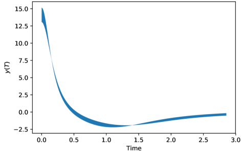
Figure 3. VNODE-LP numerical integration with solution intervals scaled up $\times 100$. The “pinch points” of near zero $y$-uncertainty occur when $\delta=y_{b}(t)\sim 0$, and although it is not shown here, the $\dot{y}$-uncertainty is larger at these points.

We now describe our procedure for the ground state and first excited state, before describing the planning and proving sections in detail. Bound states can only occur in the range $b\in(\sqrt{2},\infty)$. To prove the ground state is unique, we split this range into four intersecting intervals, $I_{1},I_{2},I_{3},I_{4}$. For instance, we can take:

$$I_{1}=(1.4,4.26),\ I_{2}=(4.25,4.43),\ I_{3}=(4.42,6.32),\ I_{4}=(6.31,\infty).$$

Now, numerical evidence shows that the ground state occurs in the range $I_{2}$. So, in the range $I_{1}$, the solution will eventually fall into the right energy well. We use VNODE-LP to prove this by splitting $I_{1}$ into smaller chunks, and verifying that in each of these chunks the energy of the solution eventually falls below zero. We deal with the range $I_{3}$ in the same way, by showing that for all $b\in I_{3}$, $y_{b}(t)$ eventually has negative energy. In the interval $I_{4}$, the solution should always have at least one zero crossing. We prove this using the equation at infinity (3.16) as discussed in §3.4. The infinite range $b\in I_{4}$ corresponds to the finite range $\beta\in(0,0.16)$, so by splitting this range into small chunks and verifying that in these chunks $w(t)$ is eventually negative, we prove that $y_{b}(t)$ eventually crosses zero for all $b\in I_{4}$. Notice that we could have replaced the interval $I_{4}$ by $I_{3}\cup I_{4}$, and it would still be true that in this range there is at least one zero crossing. We handle with $I_{3}$ separately because the numerics of ODE (3.16) are delicate near bound states, so $I_{3}$ acts as a buffer interval.

The only range left is $I_{2}$, which actually contains the ground state. We must show that $I_{2}$ contains at most one ground state, and that it contains no first or higher excited states. To this end, we use Lemmas 6 and 7 respectively. At some time $T>0$, say $T=6$, any $y_{b}(T)$ for $b\in I_{2}$ will be positive, moving in the negative direction, and small in magnitude. We use VNODE-LP to prove that $\delta_{b}(T),\dot{\delta}_{b}(T)<0$ for $b\in I_{2}$. Let $b_{0}\in I_{2}$ be a ground state. Then for any $b>b_{0}$, the mean value theorem implies that $y_{b}(T)<y_{b_{0}}(T)$ and $\dot{y}_{b}(T)<\dot{y}_{b_{0}}(T)$. By Lemma 6, $y_{b}(T)$ must cross zero. It follows that there is at most one ground state in $I_{2}$. Next, we check that the conditions of Lemma 7 are satisfied for all $y_{b}(T)$, $b\in I_{2}$. This implies that if any solution $y_{b}(t)$ does cross zero, it must fall into the left energy well, and cannot be a higher excited state. Altogether this shows that there is at most one ground state for the ODE (3.1), as desired. It also follows from this analysis that the ground state exists, so we have successfully shown the ground state exists and is unique.

We note a subtlety in this argument. A pathological issue would be that by time $T=6$, $y_{b}(T)$ crossed all the way to the left well, come back to the right well, and then started to approach $y=0$ from the right. This would kill our later attempt to prove that the second excited state is unique, because we would miss a second excited state in $I_{2}$. To deal with this, we use energy considerations to bound $|\dot{y}_{b}(t)|$, and we make small enough time steps with VNODE-LP so that the solution cannot cross zero twice in between time steps. Then, we can be sure that the number of zero crossings observed by VNODE-LP up to some time $T$ is the actual number of zero crossings for all solutions in our initial interval $\mathbf{b}$, up to time $T$.

To prove the ground state is unique, we split the range $(\sqrt{2},\infty)$ into subintervals to which we applied three different proof methods. The method for $I_{1}$ and $I_{3}$ was FALL: we proved that the solution eventually has negative energy and thus cannot be a bound state. The method for $I_{4}$ was INFTY_CROSSES_MANY, we used the equation at infinity to show that there are sufficiently many zero crossings and thus no ground states. The method for $I_{2}$ was BOUND_STATE_GOOD, we used the analytical Lemmas 6, 7 to show that there was at most one ground state and no other bound states. These are the same methods we use to deal with higher excited states. We have used the same notation here as is used in the code, for ease of verifying that the code follows the mathematical argument.

Let us extend our procedure to prove the first excited state is unique. We split up $(\sqrt{2},\infty)$ into six pieces:

$$I_{1}=(1.40,4.26),\ I_{2}=(4.25,4.43),\ I_{3}=(4.42,14.10),$$

$$I_{4}=(14.09,14.12),\ I_{5}=(14.11,16.11),\ I_{6}=(16.10,\infty).$$

We apply the FALL method to $I_{1}$, $I_{3}$, $I_{5}$, we apply the BOUND_STATE_GOOD method to $I_{2}$, $I_{4}$, and we apply the INFTY_CROSSES_MANY method to $I_{6}$. For the interval $I_{4}$, our careful stepping procedure as described above lets us find a time $T>0$, for example $T=8$, such that $y_{b}(T)$ crosses zero exactly once by time $T$ for all $b\in I_{4}$. We can also verify that $\dot{y}_{b}(T)>0$, $\delta_{b}(T)>0$, $\dot{\delta}_{b}(T)>0$, so that the conditions of Lemma 6 are satisfied and there is at most one first excited state in the interval $I_{4}$. Next we verify that the conditions of Lemma 7 are satisfied uniformly for $b\in I_{4}$ at time $T$, so that there are no second or higher excited states in $I_{4}$. Altogether this shows that the first excited state exists and is unique, and sets us up to prove subsequent excited states are unique as well.

4.2. Planning section

We now describe the planning section of the code. Given a value $N\geq 0$, this section outputs a list of intervals $I_{1},I_{2},\ldots,I_{k}$, along with which method is to be used in each interval. The proving section will use this plan to verify that all bound states up to the $N^{th}$ (that is, all bound states with $\leq N$ zero crossings, or in other words the first $N$ excited states) are unique.

Let $b_{0},b_{1},\ldots,b_{N}$ denote the locations of the first $N$ excited states (assuming for now that they are unique). We find their locations numerically with a binary search. To find $b_{k}$, we keep track of a lower bound $l<b_{k}$ and an upper bound $u>b_{k}$, and at each iteration, check how many times $y_{m}(t)$ crosses zero, $m=(l+u)/2$. If $y_{m}(t)$ crosses zero more than $k$ times, we set $u:=m$, and if not we set $l:=m$. We iterate until we have a small enough interval $(l,m)$ containing $b_{k}$.

Next, we find small enough intervals around each bound state so that the BOUND_STATE_GOOD method can run successfully for each bound state. We start with a large interval around $b_{k}$, width $~{}0.5$, and then keep on dividing the width by two until BOUND_STATE_GOOD succeeds.

Third, we fill in the space between the bound states with FALL intervals. We include a buffer interval above the last bound state so as to make INFTY_CROSSES_MANY run faster.

Finally, we create an interval $\boldsymbol{\beta}=(0,\beta)$ corresponding to the infinite interval $(1/\beta,\infty)$ where we will show the ODE crosses zero at least $N+1$ times.

4.3. Proving section

The proving section receives a list of intervals and methods from the planning section, and outputs a rigorous proof that the first $N$ excited states are unique. The first step is to verify that subsequent intervals intersect each other, so that every real number in the range $(\sqrt{2},\infty)$ is covered by some interval. Next, the different methods are implemented as follows.

The FALL method receives an interval, e.g. $(1.4,4.2)$, and must prove that for all $b$ in that interval $y_{b}(t)$ eventually has negative energy. It begins by attempting to integrate with that potentially very large input interval for $b$. Of course, VNODE-LP will likely fail to integrate with such a large input interval. If this happens, we bisect the interval into two halves, an upper and lower half, and recursively apply the FALL method to each half. Once the starting intervals are small enough, VNODE-LP will successfully integrate and prove that the energy is eventually negative. This bisection method allows us to use larger intervals away from the bound states and smaller intervals closer to the bound states, where the computations are more delicate.

The BOUND_STATE_GOOD method receives an interval $I$ which supposedly contains an $n$th bound state. It must prove that there is at most one $n$th bound state, no lower bound states, and no higher bound states in $I$. We use a careful stepping procedure to find some time $T>0$ such that for all $b\in I$, $y_{b}(t)$ crosses zero exactly $n$ times by time $T$. This already shows that $I$ doesn’t contain any lower bound states. Increasing $T$ if necessary, we also verify that $\dot{y}_{b}(T)$, $\delta_{b}(T)$, and $\dot{\delta}_{b}(T)$ all have the opposite sign as $y_{b}(T)$ uniformly in $I$. As discussed earlier, Lemma 6 then implies that there is at most one $n$th bound state in $I$. Finally, we verify that the conditions in Lemma 7 apply at time $T$, so there are no higher bound states in $I$. Throughout we use interval arithmetic, never floating point arithmetic.

The INFTY_CROSSES_MANY method works similarly to the FALL method. We bisect the interval $(0,\beta)$ into smaller pieces, and in each of these small pieces we prove that $w(t)$ has at least $N+1$ crossings.

Altogether, these methods show that if it exists, the $n$th bound state (counting from $n=0$) must be unique and lie in the $n$th BOUND_STATE_GOOD interval. This proves that all bound states up to the $N^{th}$ are unique, as desired. In fact, the code may also be used to show these bound states exist by counting crossing numbers, but this is already known by synthetic methods [10].

5. Using VNODE-LP and the data

The code and full output logs from the proof procedure can be found at https://github.com/alexander-cohen/NLKG-Uniqueness-Prover, the most recent commit at the time of writing is 9cf63c06ca1838e64dd35fe11ca4fdfd45591714. The code is contained in the single C++ file “nlkg_uniqueness_prover.cc”, and output logs are titled “uniqueness_output_N=*.txt”. The code proved the first 20 excited states are unique in $\sim 4$h running on a MacBook Pro 2017, 2.5 GHz. Time is the main limiting factor to proving uniqueness of more excited states. We summarize the output of the proof for $N=3$ excited states. Intervals are rounded for space, in actuality they have a nonempty intersection. See Figure 4 for a visual representation of the same information.

Interval	Method	Details
[1.414, 4.266]	FALL
[4.266, 4.433]	BOUND_STATE_GOOD	Bound state 0, used $T=1.921$ $y(T)\in[0.127,0.277]$ $\dot{y}(T)\in[-0.342,-0.283]$ $\delta\in[-0.374,-0.269]$ $\dot{\delta}\in[-0.139,-0.049]$
[4.433, 14.095]	FALL
[14.085, 14.115]	BOUND_STATE_GOOD	Bound state 1, used $T=2.855$ $y(T)\in-0.3[40,43]$ $\dot{y}(T)\in 0.452[46,55]$ $\delta\in 0.15[59,63]$ $\dot{\delta}\in 0.00[05,12]$
[14.115, 29.090]	FALL
[29.090, 29.174]	BOUND_STATE_GOOD	Bound state 2, used $T=4.970$ $y(T)\in 0.1[05,29]$ $\dot{y}(T)\in-0.1[34,46]$ $\delta\in-0.1[18,26]$ $\dot{\delta}\in-0.0[57,65]$
[29.174, 49.339]	FALL
[49.339, 49.381]	BOUND_STATE_GOOD	Bound state 3, used $T=5.908$ $y(T)\in-0.1[68,76]$ $\dot{y}(T)\in[0.198,0.202]$ $\delta\in 0.07[31,55]$ $\dot{\delta}\in 0.01[72,91]$
[49.381, 51.381]	FALL
[0.000, 0.019]	INFTY_CROSSES_MANY

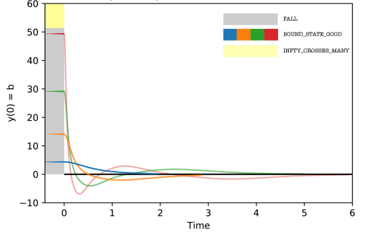
Figure 4. Graph showing first three excited states, and how the $b$-axis is partitioned by different proof methods.

References

- [1] H. Berestycki and P.-L. Lions “Nonlinear scalar field equations. I. Existence of a ground state” In Arch. Rational Mech. Anal. 82.4, 1983, pp. 313–345 DOI: 10.1007/BF00250555
- [2] H. Berestycki and P.-L. Lions “Nonlinear scalar field equations. II. Existence of infinitely many solutions” In Arch. Rational Mech. Anal. 82.4, 1983, pp. 347–375 DOI: 10.1007/BF00250556
- [3] Alexandre Cabot, Hans Engler and Sébastien Gadat “On the long time behavior of second order differential equations with asymptotically small dissipation” In Trans. Amer. Math. Soc. 361.11, 2009, pp. 5983–6017 DOI: 10.1090/S0002-9947-09-04785-0
- [4] Thierry Cazenave “Semilinear Schrödinger equations” 10, Courant Lecture Notes in Mathematics New York University, Courant Institute of Mathematical Sciences, New York; American Mathematical Society, Providence, RI, 2003, pp. xiv+323 DOI: 10.1090/cln/010
- [5] C.. Clemons and C…. Jones “A geometric proof of the Kwong-McLeod uniqueness result” In SIAM J. Math. Anal. 24.2, 1993, pp. 436–443 DOI: 10.1137/0524027
- [6] Charles V. Coffman “Uniqueness of the ground state solution for and a variational characterization of other solutions” In Arch. Rational Mech. Anal. 46, 1972, pp. 81–95 DOI: 10.1007/BF00250684
- [7] Carmen Cortázar, Marta García-Huidobro and Cecilia S. Yarur “On the uniqueness of the second bound state solution of a semilinear equation” In Annales de l’Institut Henri Poincare (C) Non Linear Analysis 26.6, 2009, pp. 2091–2110 DOI: 10.1016/j.anihpc.2009.01.004
- [8] Ovidiu Costin, Min Huang and Wilhelm Schlag “On the spectral properties of in three dimensions” In Nonlinearity 25.1, 2012, pp. 125–164 DOI: 10.1088/0951-7715/25/1/125
- [9] Matthew Creek, Roland Donninger, Wilhelm Schlag and Stanley Snelson “Linear stability of the skyrmion” In Int. Math. Res. Not. IMRN, 2017, pp. 2497–2537 DOI: 10.1093/imrn/rnw114
- [10] Stuart P. Hastings and J. McLeod “Classical methods in ordinary differential equations” With applications to boundary value problems 129, Graduate Studies in Mathematics American Mathematical Society, Providence, RI, 2012, pp. xviii+373 DOI: 10.1090/gsm/129
- [11] Man Kam Kwong “Uniqueness of positive solutions of in ” In Arch. Rational Mech. Anal. 105.3, 1989, pp. 243–266 DOI: 10.1007/BF00251502
- [12] Kevin McLeod “Uniqueness of positive radial solutions of in . II” In Trans. Amer. Math. Soc. 339.2, 1993, pp. 495–505 DOI: 10.2307/2154282
- [13] Kevin McLeod and James Serrin “Uniqueness of positive radial solutions of in ” In Arch. Rational Mech. Anal. 99.2, 1987, pp. 115–145 DOI: 10.1007/BF00275874
- [14] Kenji Nakanishi and Wilhelm Schlag “Invariant manifolds and dispersive Hamiltonian evolution equations”, Zurich Lectures in Advanced Mathematics European Mathematical Society (EMS), Zürich, 2011, pp. vi+253 DOI: 10.4171/095
- [15] Nedialko S. Nedialkov “An Interval Solver for Initial Value Problems in Ordinary Differential Equations”, 2010 URL: http://www.cas.mcmaster.ca/~nedialk/vnodelp/
- [16] Nedialko S. Nedialkov “Implementing a rigorous ODE solver through literate programming” In Modeling, design, and simulation of systems with uncertainties, Math. Eng. Springer, Heidelberg, 2011, pp. 3–19 DOI: 10.1007/978-3-642-15956-5˙1
- [17] Nedialko S. Nedialkov “VNODE-LP documentation”, 2010 URL: http://www.cas.mcmaster.ca/~nedialk/vnodelp/doc/vnode.pdf
- [18] L.. Peletier and James Serrin “Uniqueness of nonnegative solutions of semilinear equations in ” In J. Differential Equations 61.3, 1986, pp. 380–397 DOI: 10.1016/0022-0396(86)90112-9
- [19] L.. Peletier and James Serrin “Uniqueness of positive solutions of semilinear equations in ” In Arch. Rational Mech. Anal. 81.2, 1983, pp. 181–197 DOI: 10.1007/BF00250651
- [20] Gerald H. Ryder “Boundary value problems for a class of nonlinear differential equations” In Pacific J. Math. 22, 1967, pp. 477–503 URL: http://projecteuclid.org/euclid.pjm/1102992100
- [21] Walter A. Strauss “Existence of solitary waves in higher dimensions” In Comm. Math. Phys. 55.2, 1977, pp. 149–162 URL: http://projecteuclid.org/euclid.cmp/1103900983
- [22] Terence Tao “Nonlinear dispersive equations” Local and global analysis 106, CBMS Regional Conference Series in Mathematics Published for the Conference Board of the Mathematical Sciences, Washington, DC; by the American Mathematical Society, Providence, RI, 2006, pp. xvi+373 DOI: 10.1090/cbms/106
- [23] W.C Troy “The existence and uniqueness of bound-state solutions of a semi-linear equation” In Proceedings of the Royal Society A: Mathematical, Physical and Engineering Sciences 461.2061, 2005, pp. 2941–2963 DOI: 10.1098/rspa.2005.1482
- [24] Li Qun Zhang “Uniqueness of positive solutions to semilinear elliptic equations” In Acta Math. Sci. (Chinese) 11.2, 1991, pp. 130–142