On The Impact Of ²²Ne On The Pulsation Periods Of Carbon-Oxygen White Dwarfs With Helium Dominated Atmospheres

Abstract

We explore changes in the adiabatic low-order g-mode pulsation periods of 0.526, 0.560, and 0.729 $\mathrm{M}_{\odot}$ carbon-oxygen white dwarf models with helium-dominated envelopes due to the presence, absence, and enhancement of $\mathrm{{}^{22}Ne}$ in the interior. The observed g-mode pulsation periods of such white dwarfs are typically given to 6$-$7 significant figures of precision. Usually white dwarf models without $\mathrm{{}^{22}Ne}$ are fit to the observed periods and other properties. The root-mean-square residuals to the $\simeq$ 150$-$400 s low-order g-mode periods are typically in the range of $\sigma_{\rm rms}$ $\lesssim$ 0.3 s, for a fit precision of $\sigma_{\rm rms}/P$ $\lesssim$ 0.3%. We find average relative period shifts of $\Delta P/P$ $\simeq$ $\pm$ 0.5% for the low-order dipole and quadrupole g-mode pulsations within the observed effective temperature window, with the range of $\Delta P/P$ depending on the specific g-mode, abundance of $\mathrm{{}^{22}Ne}$, effective temperature, and mass of the white dwarf model. This finding suggests a systematic offset may be present in the fitting process of specific white dwarfs when $\mathrm{{}^{22}Ne}$ is absent. As part of the fitting processes involves adjusting the composition profiles of a white dwarf model, our study on the impact of $\mathrm{{}^{22}Ne}$ can provide new inferences on the derived interior mass fraction profiles. We encourage routinely including $\mathrm{{}^{22}Ne}$ mass fraction profiles, informed by stellar evolution models, to future generations of white dwarf model fitting processes.

1 Introduction

Photons emitted from stellar surfaces and neutrinos released from stellar interiors may not directly reveal all that we want to know about the internal constitution of the stars. For example, a direct view of the chemical stratification from the core to the surface is hidden. These interior abundance profiles matter: they impact a star’s opacity, thermodynamics, nuclear energy generation, and pulsation properties. The stellar models, in turn, are used to interpret the integrated light of stellar clusters and galaxies (e.g., Alsing et al., 2020), decipher the origin of the elements (e.g., Arcones et al., 2017; Placco et al., 2020), predict the frequency of merging neutron stars and black holes (Giacobbo & Mapelli, 2018; Farmer et al., 2020; Marchant & Moriya, 2020; Abbott et al., 2020), and decipher the population(s) of exploding white dwarfs that underlay Type Ia supernova cosmology (e.g., Miles et al., 2016; Rose et al., 2020).

Neutrino astronomy, in concert with stellar models, can probe the isotopic composition profiles in energy producing regions of the Sun (Borexino Collaboration et al., 2018, 2020) and nearby ($d$ $\lesssim$ 1 kpc) presupernova massive stars up to tens of hours before core-collapse (e.g., Patton et al., 2017; Simpson et al., 2019; Mukhopadhyay et al., 2020). Stellar seismology, also in concert with stellar models, can probe the elemental composition profiles in pulsating stars from the upper main-sequence (e.g., Simón-Díaz et al., 2018; Pedersen et al., 2019; Balona & Ozuyar, 2020) through the red-giant branch (e.g., Hekker & Christensen-Dalsgaard, 2017; Hon et al., 2018) to white dwarfs (WDs, e.g., Hermes et al., 2017; Giammichele et al., 2018; Córsico et al., 2019; Bell et al., 2019; Bischoff-Kim et al., 2019; Althaus et al., 2020).

Most of a main-sequence star’s initial metallicity $Z$ comes from the carbon-nitrogen-oxygen (CNO) and $\mathrm{{}^{56}Fe}$ nuclei inherited from its ambient interstellar medium. All of the CNO piles up at $\mathrm{{}^{14}N}$ when H-burning on the main-sequence is completed because the $\mathrm{{}^{14}N}$($p$,$\gamma$)$\mathrm{{}^{15}O}$ reaction rate is the slowest step in the H-burning CNO cycle. During the ensuing He-burning phase, all of the ¹⁴N is converted to ²²Ne by the reaction sequence $\mathrm{{}^{14}N}$($\alpha$,$\gamma$)¹⁸F(,$e^{+}\nu_{e}$)¹⁸O($\alpha$,$\gamma$)$\mathrm{{}^{22}Ne}$. The abundance of $\mathrm{{}^{22}Ne}$ when He-burning is completed is thus proportional to the initial CNO abundance of the progenitor main-sequence star. The weak reaction in this sequence powers the neutrino luminosity during He-burning (e.g., Serenelli & Fukugita, 2005; Farag et al., 2020) and marks the first time in a star’s life that the core becomes neutron rich. For zero-age main sequence (ZAMS) masses between $\simeq$ 0.5 $\mathrm{M}_{\odot}$ (Demarque & Mengel, 1971; Prada Moroni & Straniero, 2009; Gautschy, 2012) and $\simeq$ 7 $\mathrm{M}_{\odot}$ (Becker & Iben, 1979, 1980; García-Berro et al., 1997), depending on the treatment of convective boundary mixing (Weidemann, 2000; Denissenkov et al., 2013; Jones et al., 2013; Farmer et al., 2015; Lecoanet et al., 2016; Constantino et al., 2015, 2016, 2017), the $\mathrm{{}^{14}N}$($\alpha$,$\gamma$)¹⁸F(,$e^{+}\nu_{e}$)¹⁸O($\alpha$,$\gamma$)$\mathrm{{}^{22}Ne}$ reaction sequence determines the $\mathrm{{}^{22}Ne}$ content of a resulting carbon-oxygen white dwarf (CO WD). We follow the convention that $\mathrm{{}^{22}Ne}$ is the “metallicity” of the CO WD.

Camisassa et al. (2016) analyze the impact of $\mathrm{{}^{22}Ne}$ on the sedimentation and pulsation properties of H-dominated atmosphere WDs (i.e., the DAV class of WD) with masses of 0.528, 0.576, 0.657, and 0.833 $\mathrm{M}_{\odot}$. These WD models result from $Z$ = 0.02 non-rotating evolutionary models that start from the ZAMS and are evolved through the core-hydrogen and core-helium burning, thermally pulsing asymptotic giant branch (AGB), and post-AGB phases. At low luminosities, $\log(L/\mathrm{L}_{\odot})$ $\lesssim$ $-4.5$, they find that $\mathrm{{}^{22}Ne}$ sedimentation delays the cooling of WDs by 0.7 to 1.2 Gyr, depending on the WD mass. They also find that $\mathrm{{}^{22}Ne}$ sedimentation induces differences in the periods that are larger than the present observational uncertainties.

Giammichele et al. (2018) analyze in their supplemental material the effect of $\mathrm{{}^{22}Ne}$ on the pulsation periods of a 0.570 $\mathrm{M}_{\odot}$ template-based model for the DB WD KIC 08626021. They considered a model consisting of pure oxygen core surrounded by a pure helium envelope with the same mass and effective temperature equal to those inferred for KIC 08626021. Next, they considered a model that replaces the pure oxygen core with an oxygen-dominated core plus a trace amount of $\mathrm{{}^{22}Ne}$. They find that the model with $\mathrm{{}^{22}Ne}$ has, on average, shorter pulsation periods.

This article is novel in three ways. One, we explore the impact of $\mathrm{{}^{22}Ne}$ on the adiabatic low-order g-mode pulsation periods of CO WD models with a He-dominated atmosphere (i.e., the DBV class of WD) as the models cool through the range of observed DBV effective temperatures. Two, we derive an approximation formula for the Brunt-Väisälä frequency in WDs that allows new physical insights into why the low-order g-mode pulsation periods change due to the presence, and absence, of $\mathrm{{}^{22}Ne}$. Three, we analyze how the $\mathrm{{}^{22}Ne}$ induced changes in the pulsation periods depend on the mass and temporal resolutions of the WD model. Our explorations can help inform inferences about the interior mass fraction profiles derived from fitting the observed periods of specific DBV WDs (e.g., Metcalfe et al., 2002; Fontaine & Brassard, 2002; Metcalfe, 2003; Metcalfe et al., 2003; Hermes et al., 2017; Giammichele et al., 2017, 2018; Charpinet et al., 2019; De Gerónimo et al., 2019; Bischoff-Kim et al., 2019).

In Section 2 we summarize the input physics, and discuss in detail the chemical stratification, cooling properties, and g-mode pulsation periods of one DBV WD model. In Section 3 we present our results on changes to the low-order g-mode pulsation periods due to the presence, or absence, of $\mathrm{{}^{22}Ne}$ from this model. In Section 4 we study changes in the g-mode pulsation periods due to $\mathrm{{}^{22}Ne}$ from a less massive and a more massive WD model. In Section 5 we summarize and discuss our results. In Appendix A we study the robustness of our results with respect to mass and temporal resolution, and in Appendix B we discuss in more depth some of the input physics.

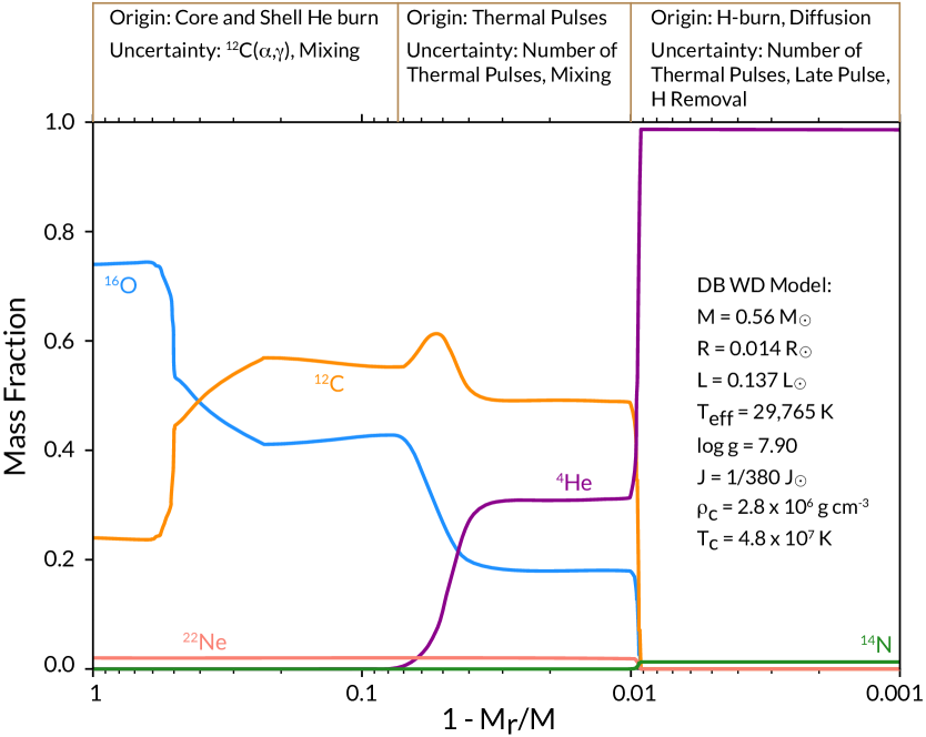
Figure 1: Mass fraction profiles of the 0.56 $\mathrm{M}_{\odot}$DB WD resulting from the evolution of the 2.1 $\mathrm{M}_{\odot}$, $Z$=0.02, ZAMS model.

2 A Baseline WD Model

2.1 Input Physics

We use MESA version r12115 (Paxton et al., 2011, 2013, 2015, 2018, 2019) to evolve a $2.1\,\mathrm{M}_{\odot}$, $Z$ = 0.02 metallicity model from the ZAMS through core H-burning and core He-burning. After winds during the thermal pulses on the AGB have reduced the H-rich envelope mass to $0.01\,\mathrm{M}_{\odot}$, the remaining hydrogen is stripped from the surface to form a young, 0.56 $\mathrm{M}_{\odot}$DB WD. This model is tuned to match the observed and inferred properties of KIC 08626021 (Bischoff-Kim et al., 2014; Giammichele et al., 2018; Timmes et al., 2018; Charpinet et al., 2019; De Gerónimo et al., 2019). Additional details of the input physics are given in Appendix B, and the MESA r12115 files to reproduce our work are available at https://doi.org/10.5281/zenodo.4338180 (catalog https://doi.org/10.5281/zenodo.4338180)

2.2 Mass Fraction Profiles

Figure 1 shows the mass fraction $X(^{A}Z)$ profiles of the resulting 0.56 $\mathrm{M}_{\odot}$DB WD model, where $A$ is the number of nucleons and $Z$ is the number of protons. Brown boxes divide the mass fraction profiles into three regions according to their origins and uncertainties. The $X(\mathrm{{}^{12}C})$ and $X(\mathrm{{}^{16}O})$ profiles in the innermost $\simeq$ 90% by mass region are determined during core and shell He-burning. The main uncertainties in this region are the $\mathrm{{}^{12}C}$($\alpha$,$\gamma$)$\mathrm{{}^{16}O}$ reaction rate (e.g., deBoer et al., 2017), and the treatment of convective mixing boundaries during core H-and He-burning (e.g., Constantino et al., 2015, 2016, 2017).

The CO and $X(\mathrm{{}^{4}He})$ profiles between $\simeq$ 1% and $\simeq$ 10% of the exterior WD mass originate from shell He-burning during the thermal pulse phase of evolution on the AGB. Most of the total He mass is held in this region. The primary uncertainties in this region are the number of thermal pulses and convective boundary layer mixing. The number of thermal pulses a model undergoes is sensitive to the mass resolution, time resolution, mass loss rate, and the treatment of convective boundaries (Iben & Renzini, 1983; Herwig, 2005; Karakas & Lattanzio, 2014). The sharp change in all the mass fractions at $\simeq$ 1% of the exterior WD mass marks the extent reached by the convective boundary during the last thermal pulse.

CO profiles in this region may also be subject to other mixing processes. For example, the magnitude of the $X(\mathrm{{}^{12}C})$ “bump” is subject to the strength and duration of the thermohaline instability, which occurs when material is stable to convection according to the Ledoux criterion, but has an inverted molecular weight gradient (Baines & Gill, 1969; Brown et al., 2013; Garaud, 2018; Bauer & Bildsten, 2018).

The $X(\mathrm{{}^{4}He})$ profile of the outer $\simeq$ 0.1% to 1% of the WD mass is determined by shell H-burning. All of the initial CNO mass fractions have been converted to $\mathrm{{}^{14}N}$. The main uncertainties in this region are the number of thermal pulses during the AGB phase of evolution, late or very late thermal pulses (Bloecker, 1995a, b; Blöcker, 2001), and mechanisms to remove the residual high entropy, H-rich layer to produce a DB WD from single and binary evolution (e.g., D’Antona & Mazzitelli, 1990; Althaus & Benvenuto, 1997; Parsons et al., 2016).

The $X(\mathrm{{}^{22}Ne})$ profile is essentially flat and spans the inner $\simeq$ 99% by mass. As discussed in Section 1, $X(\mathrm{{}^{22}Ne})$ is created from $\mathrm{{}^{14}N}$ during He-burning.

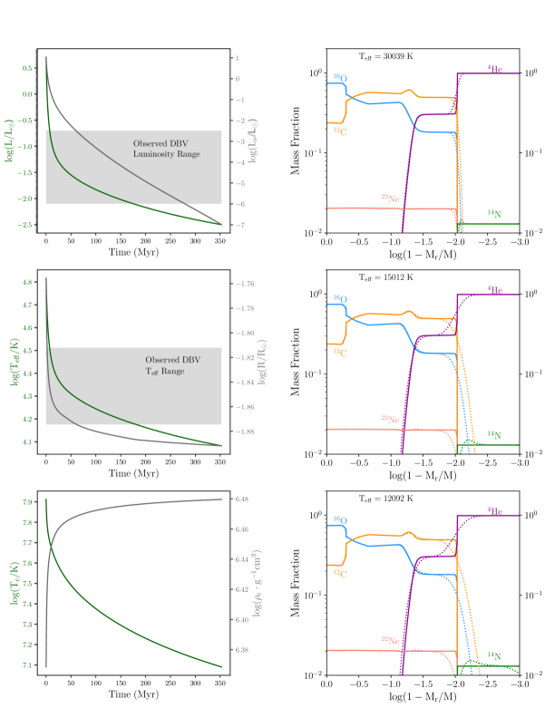
Figure 2: Evolution of baseline model’s photon luminosity $L$ and neutrino luminosity $L_{\nu}$ (left top), effective temperature $T_{\rm eff}$ and radius $R$ (left middle), central temperature $T_{c}$ and central density $\rho_{c}$ (left bottom). Time begins a few thermal timescales after the ab initio WD is released. Gray bands show the luminosity and $T_{\rm eff}$ range of currently observed DBV WD (Montreal White Dwarf Database, Dufour et al., 2017). Mass fraction profiles are shown at $T_{\rm eff}$ = 30,039 K (right top), 15,012 K (right middle), and 12,092 K (right bottom) and at the end of the evolution. Initial mass fraction profiles are shown as solid curves and the diffusing mass fraction profiles are shown as dotted curves.

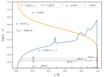
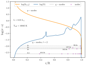
Figure 3: Propagation diagram for the dipole $\ell$ = 1 (top) and quadrupole $\ell$ = 2 (bottom) g-modes at $L$ = 0.01 $\mathrm{L}_{\odot}$ for the baseline WD model. The Lamb frequency ($S_{\ell}$, orange), Brunt-Väisälä frequency ($N$, blue), radial order $n$ = 1,2,3,10 eigenfrequencies (dotted black lines), nodes in the radial eigenfunction (filled circles), and g-mode period of each radial order are labeled.

2.3 Constructing Ab Initio White Dwarf Models

Starting from a set of pre-main sequence (pre-MS) initial conditions, accurate predictions for the properties of the resulting WD model, especially the mass fraction profiles, do not exist due to the nonlinear system of equations being approximated. In addition, evolving a stellar model from the pre-MS to a WD can be resource intensive. It can thus be useful for systematic studies to build ab initio WD models (e.g., WDEC, Bischoff-Kim & Montgomery, 2018). By ab initio we mean calculations that begin with a WD model, as opposed to a WD model that is the result of a stellar evolution calculation from the pre-MS. A potential disadvantage (or advantage) of ab initio WD models is the imposed initial mass fraction profiles may not be attainable by a stellar model evolved from the pre-MS. Throughout the remainder of this article we use a new capability, wd_builder, to construct ab initio WD models in MESA of a given mass and chemical stratification.

The initial structure of an ab initio WD model is approximated as an isothermal core and a radiative envelope in hydrostatic equilibrium. Here we specify an initial WD mass of 0.56 $\mathrm{M}_{\odot}$, the same WD mass as produced by the stellar evolution calculation. The imposed $X(\mathrm{{}^{4}He})$, $X(\mathrm{{}^{12}C})$, $X(\mathrm{{}^{14}N})$, $X(\mathrm{{}^{16}O})$, and $X(\mathrm{{}^{22}Ne})$ profiles are taken from the stellar evolution derived mass fraction profiles of Figure 1 and normalized to sum to unity in each cell. Henceforth we refer to this ab initio WD model as the “baseline model”.

For ab initio WD models we use He-dominated, $\log$(H/He) = $-$5.0, model atmosphere tables spanning 5,000 K $\leq$ $T_{\rm eff}$ $\leq$ 40,000 K that were provided by Odette Toloza (2019, private communication) using the Koester WD atmosphere software instrument (Koester, 2010). These tabulated atmospheres for DB WDs are publicly available as a standard atmosphere option as of MESA r12115. In addition, we use five element classes for the diffusion classes – $\mathrm{{}^{4}He}$, $\mathrm{{}^{12}C}$, $\mathrm{{}^{14}N}$ $\mathrm{{}^{16}O}$, and $\mathrm{{}^{22}Ne}$. Otherwise, all of the physics implementations and modeling choices are as described in Section 2.1.

The initial baseline model is then evolved with MESA. As the model is not in thermal equilibrium, there is an initial transient phase lasting a few thermal timescales that is disregarded. The thermal timescale is $\tau_{\rm th}$ $\simeq$ $E_{\rm th}/L_{\rm tot}$ $\simeq$ 0.67 Myr, where $E_{\rm th}$ is the thermal energy of the WD and $L_{\rm tot}$ is the photon plus neutrino luminosity. Specifically, we set the zero point to be 1.5 thermal timescales ($\simeq$  1 Myr) after the transient reaches its peak luminosity. The evolution terminates when $L_{\rm tot}$ falls below $\log(L/\mathrm{L}_{\odot})$ = $-$2.5.

Figure 2 shows the cooling properties of the baseline model. Plasmon neutrino emission dominates the energy loss budget at $T_{\rm eff}\gtrsim 25,000\,{\rm K}$ (e.g., Vila, 1966; Kutter & Savedoff, 1969; Winget et al., 2004; Bischoff-Kim & Montgomery, 2018). Photons leaving the WD surface begin to dominate the cooling as the electrons transition to a strongly degenerate plasma (van Horn, 1971). The luminosity becomes proportional to the enclosed mass, $L_{r}$ $\propto$ $\,M_{r}$, in this model only when $T_{\rm eff}\lesssim 20,000\,{\rm K}$ (Timmes et al., 2018). Energy transport in the interior is dominated by conduction, driven primarily by electron-ion scattering. Energy transport in the outer layers is dominated by radiation or convection associated with the partial ionization of He at $T_{\rm eff}\simeq 30,000\,{\rm K}$.

Figure 2 also shows the diffusion of the initial mass fractions as the baseline WD model cools to $T_{\rm eff}$ = 30,000 K, 15,000 K and 12,138 K (corresponding to the termination at $\log(L/\mathrm{L}_{\odot})$ = $-$2.5). Element diffusion of $\mathrm{{}^{22}Ne}$ is modest for the baseline 0.56 $\mathrm{M}_{\odot}$ DB WD model. Depletion of the $\mathrm{{}^{22}Ne}$ mass fraction at $\log(1-M_{r}/M$) $\simeq$ $-1.9$ has occurred by the time the model has cooled to $T_{\rm eff}$ $\simeq$ 30,000 K. As the model cools further, the surface regions in the tail of the He-dominated layer further deplete and a small $\mathrm{{}^{22}Ne}$ bump forms and propagates inwards toward the center. The timescale for $\mathrm{{}^{22}Ne}$ to travel from near the surface to the center of this WD model is $\tau_{\rm D}\simeq 2\bar{Z}\Gamma^{1/3}\rho_{6}^{-1/2}\ {\rm Gyr}\simeq 30\ {\rm Gyr}$ (Isern et al., 1991; Bravo et al., 1992; Bildsten & Hall, 2001; Deloye & Bildsten, 2002; Camisassa et al., 2016), where $\bar{Z}$ is the mean charge of the material, $\Gamma$ is the electrostatic to thermal energy ratio, and $\rho_{6}$ is the baryon mass density in units of 10⁶ g cm^-3. Thus, the $X(\mathrm{{}^{22}Ne})$ profile does not significantly change as the 0.56 $\mathrm{M}_{\odot}$baseline model evolves to $\log(L/\mathrm{L}_{\odot})$ = $-$2.5 in $\simeq$ 350 Myr. More massive WDs show larger amounts of $\mathrm{{}^{22}Ne}$ sedimentation over the same time period (Camisassa et al., 2016). WD cooling data suggests a significant enhancement due to to $\mathrm{{}^{22}Ne}$ diffusion (Cheng et al., 2019; Bauer et al., 2020), but does not effect the baseline model until it cools to effective temperatures lower than considered here ($T_{\rm eff}$ $\lesssim$ 10,000 K).

2.4 Pulsation Periods of the Baseline Model

Having established the structural and composition profiles of a cooling baseline WD model, we now consider the g-mode pulsation periods. Some of the material is classic (e.g., Unno et al., 1989; Fontaine & Brassard, 2008), but we also derive and verify the accuracy of an approximation formula for the Brunt-Väisälä frequency in WDs that allows physical insights into why the low-order g-mode pulsation periods change due to variations in the mass fraction of $\mathrm{{}^{22}Ne}$. This material is essential for establishing that the baseline model, before introducing any modifications to the chemical profiles, produces pulsation periods that are commensurate with the observations of DBV WDs.

Figure 3 shows the propagation diagram (e.g., Unno et al., 1989) for the baseline WD model after it has cooled to $T_{\rm eff}$ = 16,045 K and dimmed to $L$ = 0.01 $\mathrm{L}_{\odot}$, within the DBV WD observation window. Adiabatic pulsation frequencies are calculated using release 5.2 of the GYRE software instrument (Townsend & Teitler, 2013; Townsend et al., 2018). For a fixed radial overtone number, the $\ell$ = 1 periods are $\sim$ $\sqrt{3}$ longer than the $\ell$ = 2 periods, due to the local dispersion relation for low-frequency g-modes $\sigma_{g}$ scaling as

$$\sigma_{g}^{2}\simeq\ell(\ell+1)N^{2}/(k_{r}^{2}r^{2})\ ,$$ (1)

where $k_{r}$ is the radial wave number. The Brunt-Väisälä frequency $N$ is

$$N^{2}=\frac{g^{2}\rho}{P}\frac{\chi_{T}}{\chi_{\rho}}(\nabla_{{\rm ad}}-\nabla_{T}+B)\ ,$$ (2)

where $g$ is the gravitational acceleration, $\rho$ is the mass density, $P$ is the pressure, $T$ is the temperature, $\chi_{T}$ is the temperature exponent $\partial({\rm ln}P)/\partial({\rm ln}\rho)|_{T,\mu_{I}}$, $\chi_{\rho}$ is the density exponent $\partial({\rm ln}P)/\partial({\rm ln}T)|_{\rho,\mu_{I}}$, $\nabla_{{\rm ad}}$ is the adiabatic temperature gradient, $\nabla_{T}$ is the actual temperature gradient, and $B$ accounts for composition gradients (e.g., Hansen & Kawaler, 1994; Fontaine & Brassard, 2008). Bumps in the $N$ profile of Figure 3 correspond to transitions in the $X(\mathrm{{}^{16}O})$, $X(\mathrm{{}^{12}C})$, and $X(\mathrm{{}^{4}He})$ profiles. The implementation of Equation 2 in MESA is described in Section 3 of Paxton et al. (2013).

An approximation for $N^{2}$ in the interiors of WDs that yields physical insights begins by assuming $\nabla_{{\rm ad}}$ is much larger than $\nabla_{T}$ and $B$. Then

$$N^{2}=\frac{g^{2}\rho}{P}\frac{\chi_{T}}{\chi_{\rho}}\nabla_{{\rm ad}}\ .$$ (3)

In the interior of a WD the ions are ideal and dominate the temperature derivatives of an electron degenerate plasma. Substituting the pressure scale height $H$ = $P/(\rho g)$ and equation 3.110 of Hansen & Kawaler (1994)

$$\chi_{T}=\frac{\rho}{P}\frac{k_{B}T}{\mu_{I}m_{p}}$$ (4)

into Equation 3 gives

$$N^{2}=\frac{1}{H^{2}\chi_{\rho}}\frac{k_{B}T}{\mu_{I}m_{p}}\nabla_{{\rm ad}}\ ,$$ (5)

where $k_{B}$ is the Boltzmann constant, $\mu_{I}$ = 1/($\sum_{i}X_{i}/A_{i})$ is the ion mean molecular weight, and $m_{p}$ is the mass of the proton. Equation 3.90 of Hansen & Kawaler (1994) shows $\nabla_{{\rm ad}}$ = $(\Gamma_{3}-1)/\Gamma_{1}$, where $\Gamma_{1}$ is the first adiabatic index and $\Gamma_{3}$ $\rightarrow$ $k_{B}/(\mu_{I}m_{p}c_{v})$ is the third adiabatic index, where in the gas phase the ideal specific heat capacity is $c_{v}$ = $3k_{B}/(2\mu_{I}m_{p})$. The sentence beneath equation 3.112 of Hansen & Kawaler (1994) thus notes that $\Gamma_{3}-1$ = 2/3 for the ions in the gas phase ($\Gamma_{3}-1$ = 1/3 in the liquid phase). Combining these expressions, yields the approximation

$$N^{2}=\frac{2}{3\Gamma_{1}\chi_{\rho}H^{2}}\frac{k_{B}T}{\mu_{I}m_{p}}\ .$$ (6)

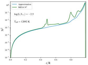
Figure 4: Comparison of the approximation for $N^{2}$ (blue curve) in Equation (6) and the full calculation of $N^{2}$ from MESA (green curve).

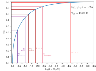
Figure 5: Mass-radius relation of the baseline DB WD model at $\log(L/\mathrm{L}_{\odot})$ = $-$2.5 with key features located: the transition from $X(\mathrm{{}^{16}O})$ to $X(\mathrm{{}^{12}C})$ dominated, the rise of $X(\mathrm{{}^{4}He})$, the $X(\mathrm{{}^{12}C})$ bump, where $S_{\ell}$ $<$ $N$ occurs, the transition to $X(\mathrm{{}^{4}He})$ dominated, and where $N^{2}$ $<$ 0.

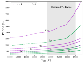
Figure 6: Period evolution of the $\ell$ = 1 (purple) and $\ell$ = 2 (green) g-modes at radial orders $n$=1,2,3,10 as the baseline model cools. Each point represents a timestep in MESA where the g-mode was calculated by GYRE. The gray band show the $T_{\rm eff}$ range of observed DBV WD.

Figure 4 compares the approximation in Equation (6) with the full $N^{2}$ calculation from MESA. The difference at $r/R$ $\simeq$ 0.5 corresponds to the $X$($\mathrm{{}^{16}O}$) $\rightarrow$ $X$($\mathrm{{}^{12}C}$) transition, at $r/R$ $\simeq$ 0.8 to the $\mathrm{{}^{12}C}$ bump, and at $r/R$ $\simeq$ 0.9 to the transition to a He dominated atmosphere. Except for the outermost layers and regions where the composition gradients are significant, the agreement is sufficient to use Equation (6) as a scaling relation for building physical insights. We always use, however, the full $N^{2}$ calculation from MESA for any quantitative analysis.

It is useful to reference features of the baseline model with respect to mass or radius. Figure 5 thus shows the mass-radius relation of the baseline model at $\log(L/\mathrm{L}_{\odot})$ = $-$2.5 with key transitions labeled.

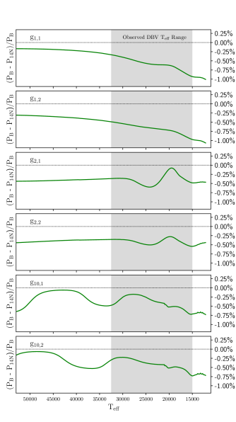
Figure 7: Top to Bottom: Relative period differences of the $g_{1,1}$, $g_{1,2}$, $g_{2,1}$, $g_{2,2}$, $g_{10,1}$ and $g_{10,2}$ modes between the baseline model, P_B, and a model where the $\mathrm{{}^{22}Ne}$ has been replaced with $\mathrm{{}^{14}N}$, P_14N. We use the notation $g_{n,\ell}$ for a g-mode of order $n$ and degree $\ell$. Gray bands show the $T_{\rm eff}$ range of currently observed DBV WDs.

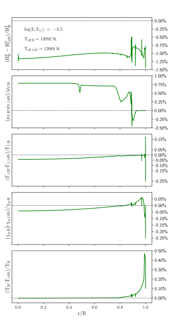
Figure 8: Top to Bottom: Relative differences in the $H^{2}$, $\mu_{I}$ $\Gamma_{1}$, $\chi_{\rho}$, and $T$ contributions to $N^{2}$ in Equation 6. Subscript B represents the baseline model, and subscript 14N represents and a model where $\mathrm{{}^{22}Ne}$ has been replaced with $\mathrm{{}^{14}N}$.

Figure 6 shows the low-order g-mode pulsation periods as the baseline WD model cools. The periods increase due to $N^{2}$ decreasing as the cooling progresses, per Equation 6. Higher radial orders have steeper slopes due to the periods scaling with $k_{r}$ in Equation 1. The increase in number of MESA models at $T_{\rm eff}$ $\simeq$ 30,000 K is due to the partial ionization of He, which leads to envelope convection in relatively hot DBV WDs. The change in slope at $T_{\rm eff}$ $\simeq$ 20,000 K is due to the luminosity becoming proportional to the enclosed mass, $L_{r}\propto M_{r}$, as the plasmon neutrino emission becomes insignificant.

In Appendix A we show that the low-order g-mode pulsation periods of the baseline model calculated with GYRE are only weakly dependent on the mass and temporal resolution of the MESA calculations.

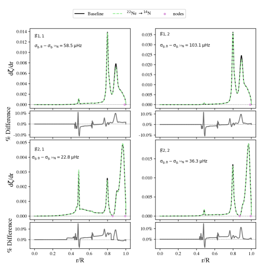
Figure 9: Weight functions of the low-order g-modes for baseline model with $\mathrm{{}^{22}Ne}$ (black curves) and a baseline model where $\mathrm{{}^{22}Ne}$ has been replaced with $\mathrm{{}^{14}N}$ (green curves). Subpanels show the relative percent differences between the two curves. The profiles shown are when the two models have cooled to $\log(L/\mathrm{L}_{\odot})$ = $-$2.5. Nodes in the radial eigenfunctions are marked by filled circles.

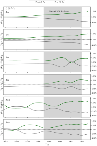
Figure 10: Top to Bottom: Relative period differences of the $g_{1,1}$, $g_{1,2}$, $g_{2,1}$, $g_{2,2}$, $g_{10,1}$ and $g_{10,2}$ modes between the baseline model, P_B, a zero-metallicity WD model (gray curves) where the $\mathrm{{}^{14}N}$ and $\mathrm{{}^{22}Ne}$ have been put into $\mathrm{{}^{4}He}$ and $\mathrm{{}^{12}C}$ respectively, and a super-solar metallicity model (green curves) where the $\mathrm{{}^{14}N}$ and $\mathrm{{}^{22}Ne}$ of the baseline model are doubled.

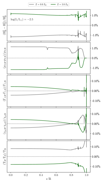
Figure 11: Top to Bottom: Relative differences in the $H^{2}$, $\mu_{I}$ $\Gamma_{1}$, $\chi_{\rho}$, and $T$ contributions to $N^{2}$ in Equation 6. Subscript B represents the baseline model, and subscript Z represents the zero-metallicity models (gray curves) and super-solar metallicity models (green curves).

3 The Impact Of $\mathrm{{}^{22}Ne}$

Having established the cooling properties and g-mode pulsation periods of a baseline model whose mass fraction profiles are from a stellar evolution model, we now explore changes in the g-mode pulsation periods due to changes in the $\mathrm{{}^{22}Ne}$ mass fraction profile shown in Figure 1. We consider three modifications: replacing $\mathrm{{}^{22}Ne}$ with $\mathrm{{}^{14}N}$, a metal-free model, and a super-solar metallicity model.

3.1 Putting the ²²Ne into ¹⁴N

Replacing $X$($\mathrm{{}^{22}Ne}$) with $X$($\mathrm{{}^{14}N}$) is a model for the reaction sequence $\mathrm{{}^{14}N}$($\alpha$,$\gamma$)¹⁸F(,$e^{+}\nu_{e}$)¹⁸O($\alpha$,$\gamma$)$\mathrm{{}^{22}Ne}$ either physically not occurring or being ignored. Figure 7 shows the relative differences in the low-order g-mode pulsation periods from this composition change. All of the relative differences are negative, implying the pulsation periods in models that exclude $\mathrm{{}^{22}Ne}$ are longer than the corresponding pulsation periods in models that include $\mathrm{{}^{22}Ne}$. The magnitude of the relative period differences span $\simeq$ 0.25%$-$1% over the range of currently observed DBV WDs, with the $g_{1,1}$ and $g_{1,2}$ modes showing the largest differences at cooler $T_{\rm eff}$. The change in the slopes at $T_{\rm eff}$ $\simeq$ 20,000 K is due to plasmon neutrino emission becoming insignificant, and thus the luminosity becoming proportional to the enclosed mass, $L_{r}\propto M_{r}$.

What drives these g-mode period changes? Replacing an isotope which has a larger mass number with an isotope which has a smaller mass number decreases $\mu_{I}$. This replacement also increases $H$ through the mechanical structure and equation of state of the CO WD. Figure 8 shows the relative differences in the $H^{2}$, $\mu_{I}$, $\Gamma_{1}$, $\chi_{\rho}$ and $T$ contributions to $N^{2}$ in Equation 6. These changes collectively determine the magnitude and sign of the period change relative to the baseline model. For this $X$($\mathrm{{}^{22}Ne}$) $\rightarrow$ $X$($\mathrm{{}^{14}N}$) model, the overall positive changes in $\mu_{I}$ and $T$ are counteracted by the negative changes from $H^{2}$, $\Gamma_{1}$, and $\chi_{\rho}$. The magnitude of the relative difference in $H^{2}$ drives the net result of a smaller $N^{2}$ and thus longer g-mode periods. The nearly uniform negative change in $H^{2}$ imply a change in the radius of the WD model. We find $(R_{B}-R_{14N})/R_{B}$ $\simeq$ $-$0.4%, meaning the $X$($\mathrm{{}^{22}Ne}$) $\rightarrow$ $X$($\mathrm{{}^{14}N}$) model has a larger radius than the model with $\mathrm{{}^{22}Ne}$. This is expected given differences in the electron fraction of a WD.

Figure 9 compares the weight functions of the baseline model with $\mathrm{{}^{22}Ne}$ and the model where the $\mathrm{{}^{22}Ne}$ has been replaced with $\mathrm{{}^{14}N}$. Following Kawaler et al. (1985), the weight function is

$$\frac{{\rm d}\zeta}{{\rm d}r}=\frac{[C({\bf y},r)+N({\bf y},r)+G({\bf y},r)]\rho r^{2}}{\int_{r=0}^{r=R}T({\bf y},r)\rho r^{2}{\rm d}r}\ ,$$ (7)

where $C({\bf y},r)$ varies with the Lamb frequency, $N({\bf y},r)$ contains the Brunt-Väisälä frequency, $G({\bf y},r)$ involves the gravitational eigenfunctions, $T({\bf y},r)$ is proportional to the kinetic energy density, and ${\bf y}=(y_{1},y_{2},y_{3},y_{4})$ are the Dziembowski (1971) variables. The frequency of an adiabatic mode is then

$$\nu^{2}=\zeta=\int_{r=0}^{r=R}\frac{{\rm d}\zeta}{{\rm d}r}\cdot{\rm d}r\ .$$ (8)

The weight function for the two models is dominated by the $N({\bf y},r)$ term except for the surface layers. Figure 9 shows that the net effect of the $\mathrm{{}^{22}Ne}$ $\rightarrow$ $\mathrm{{}^{14}N}$ composition change is a shift in $\zeta$, the area under the weight function curves, towards smaller frequencies of the low-order g-modes. The subpanels in Figure 9 illustrate the relative percent differences between the weight function curves. Most of the changes in $\zeta$ occur at the CO transition region ($r/R$ $\simeq$ 0.45, see Figure 5), $\mathrm{{}^{12}C}$ bump ($r/R$ $\simeq$ 0.8 ), and at the transition to a He-dominated atmosphere ($r/R$ $\simeq$ 0.9). The changes in these regions get as large as $\sim$ 10%. We identify the dipole g-mode of radial order $n$ = 2 as being more sensitive to the location and gradient of $\mu_{I}$ at the CO transition ($r/R$ $\simeq$ 0.5) than other low-order g-modes.

3.2 Zero-Metallicity and Super-Solar Metallicity

Replacing $X$($\mathrm{{}^{14}N}$) with $X$($\mathrm{{}^{4}He}$) and $X$($\mathrm{{}^{22}Ne}$) with $X$($\mathrm{{}^{12}C}$) is a model for ignoring the birth metallicity of the ZAMS star, CNO burning on the main-sequence, and the $\mathrm{{}^{14}N}$($\alpha$,$\gamma$)¹⁸F(,$e^{+}\nu_{e}$)¹⁸O($\alpha$,$\gamma$)$\mathrm{{}^{22}Ne}$ reaction sequence during He-burning. Most studies of the pulsation periods of observed WDs use zero-metallicity DBV WDs when deriving the interior mass fraction profiles, although see Camisassa et al. (2016) for a counterexample. Alternatively, doubling $X$($\mathrm{{}^{14}N}$) at the expense of $X$($\mathrm{{}^{4}He}$) and doubling $X$($\mathrm{{}^{22}Ne}$) at the expense of $X$($\mathrm{{}^{12}C}$) is a model for a super-solar metallicity DBV WD.

Figure 10 compares the relative change in the low-order g-mode pulsation periods of the zero and super-solar metallicity models. The period differences are negative for the zero-metallicity model and positive for the super-solar metallicity model. Zero-metallicity DBV WD models have longer periods than the baseline model, which in turn has longer periods than the super-solar metallicity model. The relative period differences of the zero and super-solar metallicity models are mostly symmetric about the baseline model’s $Z$ = 0.02 metallicity. The period differences of the zero-metallicity models, averaged over the $T_{\rm eff}$ evolution, are $\Delta P(g_{1,1})$ $\simeq$ $-$0.57 s, $\Delta P(g_{1,2})$ $\simeq$ $-$0.40 s, $\Delta P(g_{2,1})$ $\simeq$ $-$0.52 s, and $\Delta P(g_{2,2})$ $\simeq$ $-$0.40 s. For the super-solar metallicity models the averaged absolute period differences are $\Delta P(g_{1,1})$ $\simeq$ 0.66 s, $\Delta P(g_{1,2})$ $\simeq$ 0.45 s, $\Delta P(g_{2,1})$ $\simeq$ 0.46 s, and $\Delta P(g_{2,2})$ $\simeq$ 0.35 s. Over the $T_{\rm eff}$ range of currently observed DBV WDs, the mean relative period change of the dipole modes is 0.57% and the maximum of relative period change is 0.88%. The relative period change of the quadrupole modes is smaller, with a mean of 0.33% and a maximum of 0.63%.

Figure 11 shows the relative differences in the $H^{2}$, $\mu_{I}$, $\Gamma_{1}$, $\chi_{\rho}$ and $T$ contributions to $N^{2}$ of Equation 6 for the zero and super-solar metallicity models. These changes collectively determine the magnitude and sign of the period change relative to the baseline model. For the zero-metallicity models, the combined positive changes in $\mu_{I}$ and $T$ are counteracted by the collective negative changes from $H^{2}$, $\Gamma_{1}$, and $\chi_{\rho}$. The net change is negative, resulting in smaller $N^{2}$ and longer g-mode periods. Similar reasoning for the super-solar metallicity models leads to a net positive change, resulting in larger $N^{2}$ and smaller g-mode periods. The magnitude of the difference in $H^{2}$ drives the overall result for both metallicity cases. The nearly uniform changes in $H^{2}$ imply changes in the radii, and we find $(R_{B}-R_{Z})/R_{B}$ $\simeq$ $\pm$0.4% with zero-metallicity models having smaller radii and super-solar metallicity models having larger radii.

Interrogating further the composition dependence, the top panels of Figure 12 compare the mass fraction profiles of the $X$($\mathrm{{}^{22}Ne}$) $\simeq$ 0.02 baseline and zero-metallicity at 30,000 K, 15,000 K and 12,100 K as a function of mass coordinate. Element diffusion is operating in both models. The middle panels show the relative differences in these mass fraction profiles, with the $\mathrm{{}^{22}Ne}$ and $\mathrm{{}^{14}N}$ offsets zeroed out. The C and O differences at $\log(1-M_{r}/M)$ $\simeq$ $-$0.25, from Figure 5, correspond to the C/O transition at $r/R$ $\simeq$ 0.5. The He difference at $\log(1-M_{r}/M)$ $\simeq$ $-$1.0 correlates to the rise of He at $r/R$ $\simeq$ 0.75. Similarily, the C, O and He differences at $\log(1-M_{r}/M)$ $\simeq$ $-$2.0 maps to He dominating the composition at $r/R$ $\simeq$ 0.9. These relative differences are the largest at 30,000 K, reaching $\simeq$ 7.5% for $\mathrm{{}^{16}O}$ and $\simeq$ $-$6% for $\mathrm{{}^{4}He}$. The relative differences at 15,000 K and 12,100 K have about the same magnitude, $\simeq$ 7.5% for $\mathrm{{}^{16}O}$ and $\simeq$ $-$1% for $\mathrm{{}^{4}He}$. The relative mass fraction differences span a larger range of $\log(1-M_{r}/M)$ as the models cool due to element diffusion. The bottom panels of Figure 12 show the corresponding relative difference in the $\mu_{I}$ profiles. As $\mu_{I}$ is calculated by dividing the mass fraction of a isotope by its atomic weight, the relative differences in the mass fraction profiles are reduced in the $\mu_{I}$ profiles. The $\mu_{I}$ profile for 12,100 K in terms of a mass coordinate is the same as the $\mu_{I}$ profile in Figure 11 in terms of a radial coordinate.

We also computed the relative period differences between the $X$($\mathrm{{}^{22}Ne}$) $\simeq$ 0.02 baseline and zero-metallicity model with diffusion turned off to disentangle structural and diffusion effects. The results are shown in Figure 13. While there is a slight variation from the zero-metallicity gray curves shown in Figure 10, mostly in the higher order $g_{10,1}$ and $g_{10,2}$ modes, the magnitude of the relative differences remains the same. This further suggests that the period shifts are a direct consequence of the presence or absence of $\mathrm{{}^{22}Ne}$.

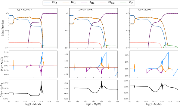
Figure 12: Top Panels: Mass fraction profiles for 0.56 $\mathrm{M}_{\odot}$baseline (colored curves) and zero metallicity (black dashed curves) models at $T_{\rm eff}$ $\simeq$ 30,000 K, 15,000 K, and 12,100 K. Middle Panels: Relative differences in mass fraction profiles, where we have zeroed out the $\mathrm{{}^{22}Ne}$ and $\mathrm{{}^{14}N}$ offsets from $\mathrm{{}^{12}C}$ and $\mathrm{{}^{4}He}$ respectively. Bottom Panel: Relative differences in $\mu_{I}$.

Figure 13: Top to Bottom: Relative period differences of the $g_{1,1}$, $g_{1,2}$, $g_{2,1}$, $g_{2,2}$, $g_{10,1}$ and $g_{10,2}$ modes between the baseline model, P_B, and the zero-metallicity WD model, P_Z, with diffusion turned off.

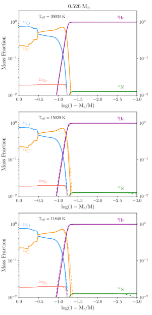
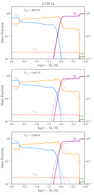
Figure 14: Mass fractions profiles for 0.52 $\mathrm{M}_{\odot}$(left column) and 0.73 $\mathrm{M}_{\odot}$(right column) ab initio DB WD models at $T_{\rm eff}$ $\simeq$ 30,000 K (top), 15,000 K (middle), and at the end of the evolution (bottom). Initial mass fraction profiles are shown as solid curves and the diffusing mass fraction profiles are shown as dotted curves.

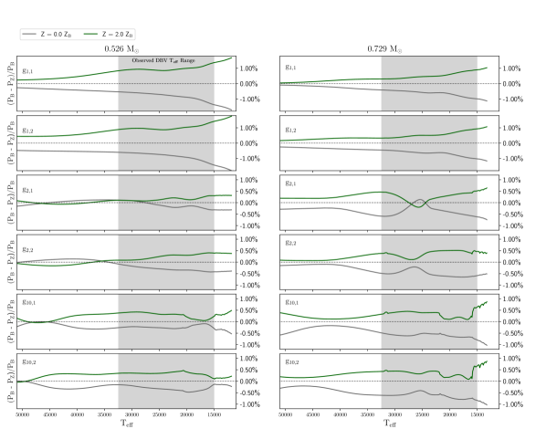
Figure 15: Relative period differences of the $g_{1,1}$, $g_{1,2}$, $g_{2,1}$, $g_{2,2}$, $g_{10,1}$ and $g_{10,2}$ modes for 0.526 $\mathrm{M}_{\odot}$(left column) and 0.729 $\mathrm{M}_{\odot}$(right column). Differences are between the baseline model, P_B, a zero-metallicity WD model (gray curves) where the $\mathrm{{}^{14}N}$ and $\mathrm{{}^{22}Ne}$ have been put into $\mathrm{{}^{4}He}$ and $\mathrm{{}^{12}C}$ respectively, and a super-solar metallicity model (green curves) where the $\mathrm{{}^{14}N}$ and $\mathrm{{}^{22}Ne}$ of the baseline model are doubled.

4 Trends in the period changes with the white dwarf mass

Using the same physics and numerical choices as for the 0.56 $\mathrm{M}_{\odot}$ baseline model, we evolved a $Z$ = 0.02, 1.1 $\mathrm{M}_{\odot}$ ZAMS stellar model from the pre-main sequence to a 0.526 $\mathrm{M}_{\odot}$ DB WD, and a $Z$ = 0.02, 3.6 $\mathrm{M}_{\odot}$ ZAMS model to a 0.729 $\mathrm{M}_{\odot}$ DB WD. This initial to final mass mapping is similar to Table 1 of Camisassa et al. (2016). Relative to the 0.56 $\mathrm{M}_{\odot}$ baseline model, the 0.526 $\mathrm{M}_{\odot}$ WD model has a thicker He-layer and a more abbreviated extent of $X$($\mathrm{{}^{22}Ne}$). Conversely, the 0.729 $\mathrm{M}_{\odot}$ WD model has a smaller $\mathrm{{}^{12}C}$ bump, a thinner He-layer, and a more extended $X$($\mathrm{{}^{22}Ne}$) profile. These mass fraction profiles were imposed on 0.526 $\mathrm{M}_{\odot}$and 0.729 $\mathrm{M}_{\odot}$ ab initio WD models, respectively.

Figure 14 shows the diffusion of these initial mass fraction profiles as the ab initio WD models cool to $T_{\rm eff}$ $\simeq$ 30,000 K, then $\simeq$ 15,000 K and finally $\simeq$ 12,000 K (corresponding to the termination at $\log(L/\mathrm{L}_{\odot})$ = $-$2.5). Element diffusion is more pronounced for the more massive 0.729 $\mathrm{M}_{\odot}$ DB WD model due to its larger surface gravity. An enhancement forms in the $X$($\mathrm{{}^{22}Ne}$) profile at $\log(1-M_{r}/M$) $\simeq$ $-2.0$ by the time the 0.729 $\mathrm{M}_{\odot}$ model has cooled to $T_{\rm eff}$ $\simeq$ 30,000 K. As the model further cools, the $X$($\mathrm{{}^{22}Ne}$) bump grows in amplitude as it propagates inwards toward the center through the He-dominated outer layers. The $X$($\mathrm{{}^{22}Ne}$) bump generates an increase in the local $N^{2}$ in the regions it propagates through from a locally larger $\mu_{I}$ and a smaller compensating $H^{2}$. The regions trailing the $X$($\mathrm{{}^{22}Ne}$) bump are depleted of $X$($\mathrm{{}^{22}Ne}$), causing a decrease in the local $N^{2}$ in these regions.

We find longer low-order g-mode periods for the more massive WD, consistent with Camisassa et al. (2016). As was done for the 0.56 $\mathrm{M}_{\odot}$ baseline model, we replace $X$($\mathrm{{}^{14}N}$) with $X$($\mathrm{{}^{4}He}$) and $X$($\mathrm{{}^{22}Ne}$) with $X$($\mathrm{{}^{12}C}$) to generate a zero-metallicity ab initio DB WD model. We also double $X$($\mathrm{{}^{14}N}$) at the expense of $X$($\mathrm{{}^{4}He}$) and double $X$($\mathrm{{}^{22}Ne}$) at the expense of $X$($\mathrm{{}^{12}C}$) to generate a super-solar metallicity DB WD.

Figure 15 compares the relative change in the low-order g-mode pulsation periods of the zero and super-solar metallicity 0.526 $\mathrm{M}_{\odot}$ and 0.729 $\mathrm{M}_{\odot}$ DB WD models. As for the 0.56 $\mathrm{M}_{\odot}$ baseline model, the relative period differences are mostly symmetric about the reference model’s $Z$ = 0.02 metallicity. For the 0.526 $\mathrm{M}_{\odot}$ models, over the $T_{\rm eff}$ range of currently observed DBV WDs, the mean relative period change of the dipole modes is 0.99% and the maximum of relative period change is 1.43%. The relative period change of the quadrupole modes is smaller, with a mean of 0.25% and a maximum of 0.43%. For the 0.729 $\mathrm{M}_{\odot}$ models, the mean relative period change of the dipole modes is 0.65% and the maximum of relative period change is 1.02%. The relative period change of the quadrupole modes is again smaller, with a mean of 0.40% and a maximum of 0.65%. These values are commensurate with the mean and maximum relative period changes found for the 0.56 $\mathrm{M}_{\odot}$ baseline model.

There are a few trends in the relative period differences with respect to the WD mass. For the zero-metallicity $n$ = 2 and $n$ = 10 g-modes, the average relative differences in the observed T_eff range increase with increasing mass. For example, as the WD mass is increased from 0.526 M_⊙ to 0.560 M_⊙, we find the average relative period differences increase by factors of 1.74, 1.22, 2.43, and 1.46, for the g_2,1, g_2,2, g_10,1, and g_10,2 modes, respectively. As the WD mass is further increased from 0.560 M_⊙ to 0.729 M_⊙, we find additional magnification factors of 1.21, 1.29, 1.21, and 1.26, for g-modes g_2,1, g_2,2, g_10,1, and g_10,2 respectively. The absence of $\mathrm{{}^{22}Ne}$ causes a greater deviation from the reference metallicity model as the WD mass increases.

The g_2,1 and g_2,2 g-modes show a trend in the local minimum as the WD mass increases. For the 0.526 M_⊙ model, the g_2,1 g-mode has a local minimum at $T_{\rm eff}$ $\lessapprox$ 20,000 K. For the 0.526 M_⊙ baseline model, this local minimum crosses zero at $T_{\rm eff}$ $\simeq$ 20,000 K. For the 0.729 M_⊙ model, the local minimum is deeper and crosses zero at at $T_{\rm eff}$ $\simeq$ 25,000 K. These trends with mass are due to when energy lost by the cooling WD is no longer dominated by neutrino cooling.

5 Discussion

We explored changes in the adiabatic low-order g-mode pulsation periods of 0.526, 0.560, and 0.729 $\mathrm{M}_{\odot}$ DB WD models due to the presence, absence, and enhancement of $\mathrm{{}^{22}Ne}$ as the models cool through the observed range of effective temperatures. We found mean relative period shifts of $\Delta P/P$ $\simeq$ $\pm$ 0.5% for the low-order dipole and quadrupole g-mode pulsations within the observed effective temperature window, with a range of $\Delta P/P$ that depends on the specific g-mode, mass fraction of $\mathrm{{}^{22}Ne}$, effective temperature, and mass of the WD model. Shifts in the pulsation periods due to the presence, absence, or enhancement of $X$($\mathrm{{}^{22}Ne}$) mostly arise from a competition between the pressure scale height and ion mean molecular weight.

Low-mass DAV WDs, the ZZ Ceti class of stars, have pulsation periods in the 100$-$1500 s range (e.g., Vincent et al., 2020). Comparing low-mass DAV WDs produced from stellar evolution models with and without diffusion of $\mathrm{{}^{22}Ne}$, Camisassa et al. (2016) find that the $\mathrm{{}^{22}Ne}$ sedimentation induces mean period differences of $\simeq$ 3 s, reaching maximum period differences of $\simeq$ 11 s. For the more massive DAV WD models, where sedimentation of $\mathrm{{}^{22}Ne}$ is stronger, they find mean period differences of $\simeq$ 15 s between when diffusion is on and off, and a maximum period differences of $\simeq$ 47 s. Comparatively, our article focuses on DBV WD models, the evolution of the pulsation periods as the DBV WD models cool, and the impact of $\mathrm{{}^{22}Ne}$ being present, absent, or enhanced in the WD interior. Nevertheless, we conducted an experiment of turning element diffusion off in our 0.56 $\mathrm{M}_{\odot}$ baseline model. At $\rm\log(L/\mathrm{L}_{\odot})$ = $-2.5$, we find an absolute mean difference for $n$ = 1 to $n$ = 11 of $\simeq$ 16 s, with a maximum period difference at $n$ = 9 of $\simeq$ 56 s. This maximum difference equates to a $\simeq$ 7% relative difference between when diffusion is on and off. Our period changes are slightly higher than those found in Camisassa et al. (2016)’s 0.833 M_⊙ model, and much larger than the differences found in their 0.576 M_⊙ model. These differences could be a result of DAV versus DBV models, as DAV models have different cooling times than DBV models. In addition, Camisassa et al. (2016) computes their period differences at $\rm log(L/L_{\odot})=-2.80$ and $\rm log(L/L_{\odot})=-2.93$ for their 0.576 and 0.833 M_⊙ models, respectively. These are dimmer than the $\rm\log(L/\mathrm{L}_{\odot})$ = $-2.5$ used for our calculations. Our maximum radial order is found up to 11 at this luminosity, while Camisassa et al. (2016) uses more radial orders, with a maximum radial order of 50.

Giammichele et al. (2018) compares the g-mode pulsation periods of a pure oxygen core surrounded by a pure helium envelope with those from an oxygen-dominated core with $X$($\mathrm{{}^{22}Ne}$) = 0.02 surrounded by a pure helium envelope. They find including $\mathrm{{}^{22}Ne}$ yields shorter periods, with mean period differences of $\simeq$ 0.1%. We find a mean period shift that is about 5 times larger in our 0.56 $\mathrm{M}_{\odot}$baseline model. This difference may be caused by the contrast in the composition of the models, which in turn causes variances in the local mean molecular weight and pressure scale height scaling described by Equation 6.

Are 1% or less period differences important? The g-mode periods of observed DBV WD are found from a Fourier analysis of the photometric light curves and are typically given to 6$-$7 significant figures of precision. Usually zero-metallicity WD models (i.e., without $\mathrm{{}^{22}Ne}$) are fit to the observed g-mode periods and other properties (e.g., $T_{\rm eff}$, $\log g$). The root-mean-square residuals to the $\simeq$ 150$-$400 s low-order g-mode periods are typically in the range $\sigma_{\rm rms}$ $\lesssim$ 0.3 s (e.g., Bischoff-Kim et al., 2014), for a fit precision of $\sigma_{\rm rms}/P$ $\lesssim$ 0.3%. Our finding of a mean relative period shift of $\Delta P/P$ $\simeq$ $\pm$ 0.5% induced by including $\mathrm{{}^{22}Ne}$ in WD models suggests a systematic offset may be present in the fitting process of specific WDs when $\mathrm{{}^{22}Ne}$ is absent. As part of the fitting process involves adjusting the composition profiles of the model WD, this study on the impact of $\mathrm{{}^{22}Ne}$ can inform inferences about the derived interior mass fraction profiles. We encourage routinely including $\mathrm{{}^{22}Ne}$ mass fraction profiles, informed by stellar evolution models, to future generations of DBV WD model fitting processes.

The adiabatic low-order g-mode pulsation periods of our DB WD models depend upon simplifying assumptions in the stellar evolution calculations (e.g., convective boundary layer mixing, shellular rotation), uncertainties (e.g., mass loss history, stripping of the residual thin H layer, thickness of the He-dominated atmosphere), and unknown inherent systematics. We hypothesize that these model dependencies and systematics could mostly cancel when dividing one model result by another model result, such as when calculating the relative period shifts $\Delta P/P$. We anticipate exploring a larger range of models, similar in approach to Fields et al. (2016), to test this conjecture in future studies.

Appendix A Convergence Studies

In this appendix we demonstrate that the pulsation periods of the baseline model are only weakly dependent on the details of the mass and temporal resolution of the MESA + GYRE calculations.

A MESA parameter controlling the mass resolution is max_dq, the maximum fraction a model’s mass in one cell. That is, the minimum number of cells in a model is $N_{\rm min\ cells}$ = 1/max_dq. We use $N_{\rm min\ cells}$ = 5,000 for all the results reported. MESA can also adaptively refines its mesh based on a set of mesh functions. The maximum cell-to-cell variation of these functions is maintained around the value of the control mesh_delta_coeff. We use mesh_delta_coeff = 1 for all the results reported. Primarily as a result of these two mesh parameters, the total number of cells in the baseline model is $\simeq$ 8,000 cells.

A MESA parameter controlling the time resolution is the largest change in the central temperature allowed over a timestep, delta_lgT_cntr_limit. For all the reported results, we use delta_lgT_cntr_limit = 0.001. MESA can also adaptively adjusts the timestep based on other criteria, but this setting dominates the size of every timestep as the baseline WD model cools. The total number of timesteps in the baseline model is $\simeq$ 1,000 and varies roughly linearly with delta_lgT_cntr_limit.

Figure 16 shows changes in the low-order g-mode periods for different $N_{\rm min\ cells}$ as the models cool. The time resolution is held fixed at delta_lgT_cntr_limit = 0.001. Our standard $N_{\rm min\ cells}$ = 5,000 baseline model is the basis of the comparison and shown as the horizontal lines. A model with 10 times less mass resolution than our standard mass resolution, $N_{\rm min\ cells}$ = 500, induces maximum relative period changes of $\simeq$ 0.05% at $\simeq$ 30,000 K for $g_{1,1}$, $\simeq$ 0.07% at $\simeq$ 35,000 K for $g_{1,2}$, $\simeq$ 0.07% at $\simeq$ 45,000 K for $g_{2,1}$, and $\simeq$ 0.07% at $\simeq$ 45,000 K for $g_{2,2}$. A model with 5 times less mass resolution than our standard mass resolution, $N_{\rm min\ cells}$ = 1,000, reduces these maximum relative period changes by $\simeq$ 20%. A model with 5 times more mass resolution than our standard mass resolution, $N_{\rm min\ cells}$ = 25,000 causes maximum relative period changes of 0.000022% at $g_{1,1}$ to 0.028% at $g_{10,1}$. These maximum relative period changes are, respectively, a factor of $\simeq$ 20,000 to 20 smaller than the relative period change caused by including or excluding $\mathrm{{}^{22}Ne}$.

Figure 17 shows changes in the low-order g-mode periods for different delta_lgT_cntr_limit as the models cool. The mass resolution is held fixed at $N_{\rm min\ cells}$ = 5,000. Our standard delta_lgT_cntr_limit = 0.001 baseline model is the basis of the comparison and shown as the horizontal lines. A model with 10 times less time resolution, delta_lgT_cntr_limit = 0.01, causes maximum relative period changes of $\simeq$ $-$0.05% at $\simeq$ 50,000 K for $g_{1,1}$, $\simeq$ 0.02% at $\simeq$ 50,000 K for $g_{1,2}$, $\simeq$ $-$0.06% at $\simeq$ 40,000 K for $g_{2,1}$, $\simeq$ $-$0.05% at $\simeq$ 45,000 K for $g_{2,2}$, $\simeq$ $-$0.25% at $\simeq$ 45,000 K for $g_{10,1}$, and $\simeq$ $-$0.25% at $\simeq$ 50,000 K for $g_{10,2}$. A model with 5 times less time resolution than our standard mass resolution, delta_lgT_cntr_limit = 0.005, reduces these maximum relative period changes by $\simeq$ 10%. A model with 5 times more time resolution, delta_lgT_cntr_limit = 0.0002, has average period changes of 0.00061 s for $g_{1,1}$, $-$0.00077 s for $g_{1,2}$, 0.0034 s for $g_{2,1}$, 0.0010 s for $g_{2,2}$, 0.0021 s for $g_{10,1}$, and 0.0014 s for $g_{10,2}$. The average period changes are a factor of $\simeq$ 1000 smaller than the average period changes caused by including or excluding $\mathrm{{}^{22}Ne}$.

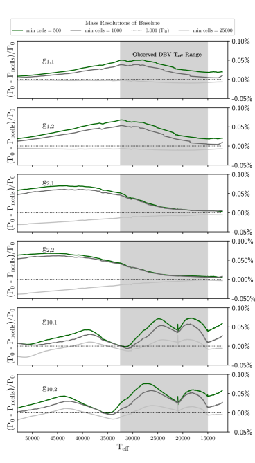
Figure 16: Relative differences in the $g_{1,1}$, $g_{1,2}$, $g_{2,1}$, $g_{2,2}$, $g_{10,1}$, $g_{10,2}$ pulsation periods for different minimum mass resolutions as the baseline WD models cool. We use the notation $g_{n,\ell}$ for a g-mode of order $n$ and degree $\ell$. The minimum mass resolution of 5,000 cells, used for all the results reported, is shown by the black horizontal lines.

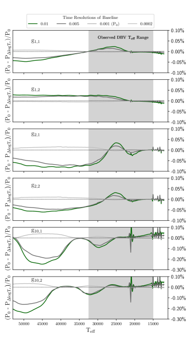
Figure 17: Relative differences in the $g_{1,1}$, $g_{1,2}$, $g_{2,1}$, $g_{2,2}$, $g_{10,1}$, and $g_{10,2}$ pulsation period for different temporal resolutions as the baseline WD models cool. The largest change in the central temperature allowed over a timestep, delta_lgT_cntr_limit = 0.001, used for all the results reported, is shown by the black horizontal lines.

Appendix B Input Physics Details

In this appendix we briefly discuss the salient physics used in our MESA models.

B.1 Thermodynamics

The MESA r12115 equation of state (EOS) is a blend of the OPAL (Rogers & Nayfonov, 2002), SCVH (Saumon et al., 1995), PTEH Pols et al. (1995), HELM (Timmes & Swesty, 2000), and PC (Potekhin & Chabrier, 2010) EOSes. The MESA EOS also covers the late stages of WD cooling where the ions in the core crystallize (e.g., Bauer et al., 2020). WD interiors lie in the PC region of the MESA EOS, which provides a semi-analytic EOS treatment for arbitrary composition. The default in MESA version 12115 is to account for each species of ion with mass fraction greater than $10^{-3}$ when calling the PC EOS. Therefore changing the interior composition in a WD model, such as including or excluding ²²Ne, self-consistently changes the thermodynamics.

B.2 Opacities

MESA r12115 divides the radiative opacity tables into two temperature regimes, low ($T$ $\lesssim$ 10⁴ K) and high ($T$ $\gtrsim$ 10⁴ K). For the stellar evolution calculations from the pre-MS to a WD we use the Ferguson et al. (2005) low-temperature regions, and for the high-temperature regions we use the OPAL Type I opacities (Iglesias & Rogers, 1996), smoothly transitioning to the OPAL Type II opacities (Iglesias & Rogers, 1996) starting at the end of core H-burning. In our WD models, the radiative opacities are provided by the OPAL Type 2 tables, which are functions of the hydrogen mass fraction X, metal mass fraction Z, and the C/O-enhancements. Thus for the same temperature and density, our $X$($\mathrm{{}^{22}Ne}$) $\rightarrow$ $X$($\mathrm{{}^{14}N}$) replacement in Section 3.1 does not change the radiative opacities. Our $X$($\mathrm{{}^{14}N}$) $\rightarrow$ $X$($\mathrm{{}^{4}He}$) and $X$($\mathrm{{}^{22}Ne}$) with $\rightarrow$ $X$($\mathrm{{}^{12}C}$) replacements to generate zero-metallicity ab initio DB WD in Section 3.2 decreases Z in the He-dominated envelope and increases the C enhancement in the interior. Conversely, our doubling $X$($\mathrm{{}^{14}N}$) at the expense of $X$($\mathrm{{}^{4}He}$) and doubling $X$($\mathrm{{}^{22}Ne}$) at the expense of $X$($\mathrm{{}^{12}C}$) to generate a super-solar metallicity ab initio DB WD in Section 3.2 increases Z in the He-dominated envelope and decreases the C enhancement in the interior. Electron conduction opacities are from Cassisi et al. (2007), which are the relevant opacity in the WD interior. The conduction opacities are a function of the mean atomic number $\bar{Z}$, which MESA evaluates using the full composition vector in each cell.

B.3 Nuclear Reaction Networks

We use MESA’s mesa_49.net, a nuclear reaction network that follows 49 isotopes from $\mathrm{{}^{1}H}$ to $\mathrm{{}^{34}S}$, including $\mathrm{{}^{22}Ne}$. This impact of this reaction network on properties of CO WDs from Monte Carlo stellar models is discussed by Fields et al. (2016). All forward thermonuclear reaction rates are from the JINA reaclib version V2.2 2017-10-20 (Cyburt et al., 2010). Inverse rates are calculated directly from the forward rates (those with positive $Q$-value) using detailed balance, rather than using fitted rates. The nuclear partition functions used to calculate the inverse rates are from Rauscher & Thielemann (2000). Electron screening factors for both weak and strong thermonuclear reactions are from Chugunov et al. (2007) with plasma parameters from Itoh et al. (1979). All the weak rates are based (in order of precedence) on the tabulations of Langanke & Martínez-Pinedo (2000), Oda et al. (1994), and Fuller et al. (1985). Thermal neutrino energy losses are from Itoh et al. (1996).

B.4 Mass Loss

The implementations of mass loss in MESA r12115 are based on a number of observationally and theoretically motivated prescriptions, but uncertainties remain on line-driven and dust-driven winds (Dupree, 1986; Willson, 2000; Boulangier et al., 2019). We follow the mass loss settings used by the MIST isochrones (Dotter, 2016; Choi et al., 2016), with a combination of the Reimer mass loss prescription (Reimers, 1975) with $\eta$=0.1 on the Red Giant Branch and a Blöcker mass loss prescription (Bloecker, 1995a) with $\eta$=0.5 on the AGB.

B.5 Rotation and Magnetic Fields

MESA r12115 implements the inherently 3D process of rotation by making the 1D shellular approximation (Zahn, 1992; Meynet & Maeder, 1997), where the angular velocity is constant over isobars. The transport of angular momentum and material due to rotationally induced instabilities is followed using a diffusion approximation (e.g., Endal & Sofia, 1978; Pinsonneault et al., 1989; Heger et al., 2000; Maeder & Meynet, 2003, 2004; Suijs et al., 2008) for the dynamical shear instability, secular shear instability, Eddington-Sweet circulation, Goldreich-Schubert-Fricke instability, and Spruit-Tayler dynamo. See Heger et al. (2000) for a description of the different instabilities and diffusion coefficients.

Magnetic fields are implemented in MESA using the formalism of Heger et al. (2005), where a magnetic torque due to a dynamo (Spruit, 2002) allows angular momentum to be transported inside the star. The azimuthal and radial components of the magnetic field are modeled as $B_{\phi}$ $\sim$ $r\sqrt{(4\pi\rho)}\omega_{A}$ and $B_{r}$ $\sim$ $B_{\phi}/(rk)$ respectively, where $r$ is the radial coordinate, $\omega_{A}$ the Alfvén frequency, and $k$ the wavenumber. These magnetic fields provide a torque $S$ = $B_{r}B_{\phi}/(4\pi)$ which slows down the rotation rate by decreasing the amount of differential rotation (Heger et al., 2005).

We initialize rotation by imposing a solid body rotation law, $\Omega/\Omega_{{\rm crit}}$ = 1.9$\times$10^-4, at the ZAMS. ZAMS is defined as where the nuclear burning luminosity is 99% of the total luminosity, and the rotation rate is normalized by the surface critical rotation rate $\Omega_{crit}$ = $\sqrt{(1-L/L_{{\rm edd}})cM/R^{3}}$, where $c$ is the speed of light, $M$ is the mass of the star, $R$ the stellar radius, $L$ the luminosity and $L_{{\rm edd}}$ the Eddington luminosity. The initial magnetic field is set to $B_{r}$ = $B_{\phi}$ = 0. Effects from rotationally induced mass loss are not included.

B.6 Element Diffusion

Element diffusion is implemented in MESA r12115 following Thoul et al. (1994), and described in Section 3 of Paxton et al. (2018). All isotopes in the reaction network are categorized into classes according to their atomic masses, each of which has a representative member whose properties are used to calculate the diffusion velocities. Diffusion coefficients are calculated, by default, according to Stanton & Murillo (2016), whose formalism is based on binary collision integrals between each pair of species in the plasma. The diffusion equation is then solved using the total mass fraction within each class. From the ZAMS to the construction of the DB WD, we use the ten element classes $\mathrm{{}^{1}H}$, $\mathrm{{}^{3}He}$, $\mathrm{{}^{4}He}$, $\mathrm{{}^{12}C}$, $\mathrm{{}^{14}N}$ $\mathrm{{}^{16}O}$, $\mathrm{{}^{20}Ne}$, $\mathrm{{}^{22}Ne}$, $\mathrm{{}^{24}Mg}$ and $\mathrm{{}^{28}Si}$.

References

- Abbott et al. (2020) Abbott, R., Abbott, T. D., Abraham, S., et al. 2020, ApJ, 900, L13, doi: 10.3847/2041-8213/aba493
- Alsing et al. (2020) Alsing, J., Peiris, H., Leja, J., et al. 2020, ApJS, 249, 5, doi: 10.3847/1538-4365/ab917f
- Althaus & Benvenuto (1997) Althaus, L. G., & Benvenuto, O. G. 1997, ApJ, 477, 313, doi: 10.1086/303686
- Althaus et al. (2020) Althaus, L. G., Gil Pons, P., Córsico, A. H., et al. 2020, arXiv e-prints, arXiv:2011.10439. https://arxiv.org/abs/2011.10439
- Arcones et al. (2017) Arcones, A., Bardayan, D. W., Beers, T. C., et al. 2017, Progress in Particle and Nuclear Physics, 94, 1, doi: 10.1016/j.ppnp.2016.12.003
- Baines & Gill (1969) Baines, P. G., & Gill, A. E. 1969, Journal of Fluid Mechanics, 37, 289, doi: 10.1017/S0022112069000553
- Balona & Ozuyar (2020) Balona, L. A., & Ozuyar, D. 2020, MNRAS, 493, 5871, doi: 10.1093/mnras/staa670
- Bauer & Bildsten (2018) Bauer, E. B., & Bildsten, L. 2018, ApJ, 859, L19, doi: 10.3847/2041-8213/aac492
- Bauer et al. (2020) Bauer, E. B., Schwab, J., Bildsten, L., & Cheng, S. 2020, arXiv e-prints, arXiv:2009.04025. https://arxiv.org/abs/2009.04025
- Becker & Iben (1979) Becker, S. A., & Iben, Jr., I. 1979, ApJ, 232, 831, doi: 10.1086/157345
- Becker & Iben (1980) —. 1980, ApJ, 237, 111, doi: 10.1086/157850
- Bell et al. (2019) Bell, K. J., Córsico, A. H., Bischoff-Kim, A., et al. 2019, A&A, 632, A42, doi: 10.1051/0004-6361/201936340
- Bildsten & Hall (2001) Bildsten, L., & Hall, D. M. 2001, ApJ, 549, L219
- Bischoff-Kim & Montgomery (2018) Bischoff-Kim, A., & Montgomery, M. H. 2018, AJ, 155, 187, doi: 10.3847/1538-3881/aab70e
- Bischoff-Kim et al. (2014) Bischoff-Kim, A., Østensen, R. H., Hermes, J. J., & Provencal, J. L. 2014, ApJ, 794, 39, doi: 10.1088/0004-637X/794/1/39
- Bischoff-Kim et al. (2019) Bischoff-Kim, A., Provencal, J. L., Bradley, P. A., et al. 2019, ApJ, 871, 13, doi: 10.3847/1538-4357/aae2b1
- Blöcker (2001) Blöcker, T. 2001, Ap&SS, 275, 1. https://arxiv.org/abs/astro-ph/0102135
- Bloecker (1995a) Bloecker, T. 1995a, A&A, 297, 727
- Bloecker (1995b) —. 1995b, A&A, 299, 755
- Borexino Collaboration et al. (2018) Borexino Collaboration, Agostini, M., Altenmüller, K., et al. 2018, Nature, 562, 505, doi: 10.1038/s41586-018-0624-y
- Borexino Collaboration et al. (2020) —. 2020, Nature, 587, 577
- Boulangier et al. (2019) Boulangier, J., Clementel, N., van Marle, A. J., Decin, L., & de Koter, A. 2019, MNRAS, 482, 5052, doi: 10.1093/mnras/sty2560
- Bravo et al. (1992) Bravo, E., Isern, J., Canal, R., & Labay, J. 1992, A&A, 257, 534
- Brown et al. (2013) Brown, J. M., Garaud, P., & Stellmach, S. 2013, ApJ, 768, 34, doi: 10.1088/0004-637X/768/1/34
- Buchler & Yueh (1976) Buchler, J. R., & Yueh, W. R. 1976, ApJ, 210, 440, doi: 10.1086/154847
- Camisassa et al. (2016) Camisassa, M. E., Althaus, L. G., Córsico, A. H., et al. 2016, ApJ, 823, 158, doi: 10.3847/0004-637X/823/2/158
- Cassisi et al. (2007) Cassisi, S., Potekhin, A. Y., Pietrinferni, A., Catelan, M., & Salaris, M. 2007, ApJ, 661, 1094
- Charpinet et al. (2019) Charpinet, S., Brassard, P., Giammichele, N., & Fontaine, G. 2019, A&A, 628, L2, doi: 10.1051/0004-6361/201935823
- Cheng et al. (2019) Cheng, S., Cummings, J. D., & Ménard, B. 2019, ApJ, 886, 100, doi: 10.3847/1538-4357/ab4989
- Choi et al. (2016) Choi, J., Dotter, A., Conroy, C., et al. 2016, ApJ, 823, 102, doi: 10.3847/0004-637X/823/2/102
- Chugunov et al. (2007) Chugunov, A. I., Dewitt, H. E., & Yakovlev, D. G. 2007, Phys. Rev. D, 76, 025028, doi: 10.1103/PhysRevD.76.025028
- Constantino et al. (2015) Constantino, T., Campbell, S. W., Christensen-Dalsgaard, J., Lattanzio, J. C., & Stello, D. 2015, MNRAS, 452, 123, doi: 10.1093/mnras/stv1264
- Constantino et al. (2017) Constantino, T., Campbell, S. W., & Lattanzio, J. C. 2017, MNRAS, 472, 4900, doi: 10.1093/mnras/stx2321
- Constantino et al. (2016) Constantino, T., Campbell, S. W., Lattanzio, J. C., & van Duijneveldt, A. 2016, MNRAS, 456, 3866, doi: 10.1093/mnras/stv2939
- Córsico et al. (2019) Córsico, A. H., Althaus, L. G., Miller Bertolami, M. M., & Kepler, S. O. 2019, A&A Rev., 27, 7, doi: 10.1007/s00159-019-0118-4
- Cyburt et al. (2010) Cyburt, R. H., Amthor, A. M., Ferguson, R., et al. 2010, ApJS, 189, 240, doi: 10.1088/0067-0049/189/1/240
- D’Antona & Mazzitelli (1990) D’Antona, F., & Mazzitelli, I. 1990, ARA&A, 28, 139, doi: 10.1146/annurev.aa.28.090190.001035
- De Gerónimo et al. (2019) De Gerónimo, F. C., Battich, T., Miller Bertolami, M. M., Althaus, L. G., & Córsico, A. H. 2019, A&A, 630, A100, doi: 10.1051/0004-6361/201834988
- deBoer et al. (2017) deBoer, R. J., Görres, J., Wiescher, M., et al. 2017, Reviews of Modern Physics, 89, 035007, doi: 10.1103/RevModPhys.89.035007
- Deloye & Bildsten (2002) Deloye, C. J., & Bildsten, L. 2002, ApJ, 580, 1077
- Demarque & Mengel (1971) Demarque, P., & Mengel, J. G. 1971, ApJ, 164, 317, doi: 10.1086/150841
- Denissenkov et al. (2013) Denissenkov, P. A., Herwig, F., Truran, J. W., & Paxton, B. 2013, ApJ, 772, 37, doi: 10.1088/0004-637X/772/1/37
- Dotter (2016) Dotter, A. 2016, ApJS, 222, 8, doi: 10.3847/0067-0049/222/1/8
- Dufour et al. (2017) Dufour, P., Blouin, S., Coutu, S., et al. 2017, in Astronomical Society of the Pacific Conference Series, Vol. 509, 20th European White Dwarf Workshop, ed. P. E. Tremblay, B. Gaensicke, & T. Marsh, 3. https://arxiv.org/abs/1610.00986
- Dupree (1986) Dupree, A. K. 1986, ARA&A, 24, 377, doi: 10.1146/annurev.aa.24.090186.002113
- Dziembowski (1971) Dziembowski, W. A. 1971, Acta Astron., 21, 289
- Endal & Sofia (1978) Endal, A. S., & Sofia, S. 1978, ApJ, 220, 279
- Farag et al. (2020) Farag, E., Timmes, F. X., Taylor, M., Patton, K. M., & Farmer, R. 2020, ApJ, 893, 133, doi: 10.3847/1538-4357/ab7f2c
- Farmer et al. (2015) Farmer, R., Fields, C. E., & Timmes, F. X. 2015, ApJ, 807, 184, doi: 10.1088/0004-637X/807/2/184
- Farmer et al. (2020) Farmer, R., Renzo, M., de Mink, S., Fishbach, M., & Justham, S. 2020, arXiv e-prints, arXiv:2006.06678. https://arxiv.org/abs/2006.06678
- Ferguson et al. (2005) Ferguson, J. W., Alexander, D. R., Allard, F., et al. 2005, ApJ, 623, 585, doi: 10.1086/428642
- Fields et al. (2016) Fields, C. E., Farmer, R., Petermann, I., Iliadis, C., & Timmes, F. X. 2016, ApJ, 823, 46, doi: 10.3847/0004-637X/823/1/46
- Fontaine & Brassard (2002) Fontaine, G., & Brassard, P. 2002, ApJ, 581, L33, doi: 10.1086/345787
- Fontaine & Brassard (2008) —. 2008, PASP, 120, 1043, doi: 10.1086/592788
- Freedman et al. (2008) Freedman, R. S., Marley, M. S., & Lodders, K. 2008, ApJS, 174, 504, doi: 10.1086/521793
- Frommhold et al. (2010) Frommhold, L., Abel, M., Wang, F., et al. 2010, Molecular Physics, 108, 2265, doi: 10.1080/00268976.2010.507556
- Fuller et al. (1985) Fuller, G. M., Fowler, W. A., & Newman, M. J. 1985, ApJ, 293, 1, doi: 10.1086/163208
- Garaud (2018) Garaud, P. 2018, Annual Review of Fluid Mechanics, 50, 275, doi: 10.1146/annurev-fluid-122316-045234
- García-Berro et al. (1997) García-Berro, E., Ritossa, C., & Iben, Jr., I. 1997, ApJ, 485, 765. http://stacks.iop.org/0004-637X/485/i=2/a=765
- Gautschy (2012) Gautschy, A. 2012, ArXiv e-prints. https://arxiv.org/abs/1208.3870
- Giacobbo & Mapelli (2018) Giacobbo, N., & Mapelli, M. 2018, MNRAS, 480, 2011, doi: 10.1093/mnras/sty1999
- Giammichele et al. (2017) Giammichele, N., Charpinet, S., Brassard, P., & Fontaine, G. 2017, A&A, 598, A109, doi: 10.1051/0004-6361/201629935
- Giammichele et al. (2018) Giammichele, N., Charpinet, S., Fontaine, G., et al. 2018, Nature, 554, 73, doi: 10.1038/nature25136
- Hansen & Kawaler (1994) Hansen, C. J., & Kawaler, S. D. 1994, Stellar Interiors. Physical Principles, Structure, and Evolution. (New York: Springer-Verlag), doi: 10.1007/978-1-4419-9110-2
- Heger et al. (2000) Heger, A., Langer, N., & Woosley, S. E. 2000, ApJ, 528, 368
- Heger et al. (2005) Heger, A., Woosley, S. E., & Spruit, H. C. 2005, ApJ, 626, 350
- Hekker & Christensen-Dalsgaard (2017) Hekker, S., & Christensen-Dalsgaard, J. 2017, A&A Rev., 25, 1, doi: 10.1007/s00159-017-0101-x
- Hermes et al. (2017) Hermes, J. J., Kawaler, S. D., Bischoff-Kim, A., et al. 2017, ApJ, 835, 277, doi: 10.3847/1538-4357/835/2/277
- Herwig (2005) Herwig, F. 2005, ARA&A, 43, 435
- Hon et al. (2018) Hon, M., Stello, D., & Zinn, J. C. 2018, ApJ, 859, 64, doi: 10.3847/1538-4357/aabfdb
- Hunter (2007) Hunter, J. D. 2007, Computing In Science & Engineering, 9, 90
- Iben & Renzini (1983) Iben, Jr., I., & Renzini, A. 1983, ARA&A, 21, 271, doi: 10.1146/annurev.aa.21.090183.001415
- Iglesias & Rogers (1996) Iglesias, C. A., & Rogers, F. J. 1996, ApJ, 464, 943
- Isern et al. (1991) Isern, J., Hernanz, M., Mochkovitch, R., & Garcia-Berro, E. 1991, A&A, 241, L29
- Itoh et al. (1996) Itoh, N., Hayashi, H., Nishikawa, A., & Kohyama, Y. 1996, ApJS, 102, 411
- Itoh et al. (1979) Itoh, N., Totsuji, H., Ichimaru, S., & Dewitt, H. E. 1979, ApJ, 234, 1079
- Jones et al. (2013) Jones, S., Hirschi, R., Nomoto, K., et al. 2013, ApJ, 772, 150, doi: 10.1088/0004-637X/772/2/150
- Karakas & Lattanzio (2014) Karakas, A. I., & Lattanzio, J. C. 2014, ArXiv e-prints. https://arxiv.org/abs/1405.0062
- Kawaler et al. (1985) Kawaler, S. D., Winget, D. E., & Hansen, C. J. 1985, ApJ, 295, 547, doi: 10.1086/163398
- Koester (2010) Koester, D. 2010, Mem. Soc. Astron. Italiana, 81, 921
- Kutter & Savedoff (1969) Kutter, G. S., & Savedoff, M. P. 1969, ApJ, 156, 1021, doi: 10.1086/150033
- Langanke & Martínez-Pinedo (2000) Langanke, K., & Martínez-Pinedo, G. 2000, Nuclear Physics A, 673, 481, doi: 10.1016/S0375-9474(00)00131-7
- Lecoanet et al. (2016) Lecoanet, D., Schwab, J., Quataert, E., et al. 2016, ApJ, 832, 71, doi: 10.3847/0004-637X/832/1/71
- Lederer & Aringer (2009) Lederer, M. T., & Aringer, B. 2009, A&A, 494, 403, doi: 10.1051/0004-6361:200810576
- Maeder & Meynet (2003) Maeder, A., & Meynet, G. 2003, A&A, 411, 543
- Maeder & Meynet (2004) —. 2004, A&A, 422, 225
- Marchant & Moriya (2020) Marchant, P., & Moriya, T. J. 2020, A&A, 640, L18, doi: 10.1051/0004-6361/202038902
- Marigo & Aringer (2009) Marigo, P., & Aringer, B. 2009, A&A, 508, 1539, doi: 10.1051/0004-6361/200912598
- Metcalfe (2003) Metcalfe, T. S. 2003, ApJ, 587, L43, doi: 10.1086/375044
- Metcalfe et al. (2003) Metcalfe, T. S., Montgomery, M. H., & Kawaler, S. D. 2003, MNRAS, 344, L88, doi: 10.1046/j.1365-8711.2003.07128.x
- Metcalfe et al. (2002) Metcalfe, T. S., Salaris, M., & Winget, D. E. 2002, ApJ, 573, 803, doi: 10.1086/340796
- Meynet & Maeder (1997) Meynet, G., & Maeder, A. 1997, A&A, 321, 465
- Miles et al. (2016) Miles, B. J., van Rossum, D. R., Townsley, D. M., et al. 2016, ApJ, 824, 59, doi: 10.3847/0004-637X/824/1/59
- Mukhopadhyay et al. (2020) Mukhopadhyay, M., Lunardini, C., Timmes, F. X., & Zuber, K. 2020, ApJ, 899, 153, doi: 10.3847/1538-4357/ab99a6
- Oda et al. (1994) Oda, T., Hino, M., Muto, K., Takahara, M., & Sato, K. 1994, Atomic Data and Nuclear Data Tables, 56, 231, doi: 10.1006/adnd.1994.1007
- Parsons et al. (2016) Parsons, S. G., Rebassa-Mansergas, A., Schreiber, M. R., et al. 2016, MNRAS, 463, 2125, doi: 10.1093/mnras/stw2143
- Patton et al. (2017) Patton, K. M., Lunardini, C., Farmer, R. J., & Timmes, F. X. 2017, ApJ, 851, 6, doi: 10.3847/1538-4357/aa95c4
- Paxton et al. (2011) Paxton, B., Bildsten, L., Dotter, A., et al. 2011, ApJS, 192, 3, doi: 10.1088/0067-0049/192/1/3
- Paxton et al. (2013) Paxton, B., Cantiello, M., Arras, P., et al. 2013, ApJS, 208
- Paxton et al. (2015) Paxton, B., Marchant, P., Schwab, J., et al. 2015, ApJS, 220, 15, doi: 10.1088/0067-0049/220/1/15
- Paxton et al. (2018) Paxton, B., Schwab, J., Bauer, E. B., et al. 2018, ApJS, 234, 34, doi: 10.3847/1538-4365/aaa5a8
- Paxton et al. (2019) Paxton, B., Smolec, R., Schwab, J., et al. 2019, ApJS, 243, 10, doi: 10.3847/1538-4365/ab2241
- Pedersen et al. (2019) Pedersen, M. G., Chowdhury, S., Johnston, C., et al. 2019, ApJ, 872, L9, doi: 10.3847/2041-8213/ab01e1
- Pinsonneault et al. (1989) Pinsonneault, M. H., Kawaler, S. D., Sofia, S., & Demarque, P. 1989, ApJ, 338, 424
- Placco et al. (2020) Placco, V. M., Santucci, R. M., Yuan, Z., et al. 2020, arXiv e-prints, arXiv:2006.04538. https://arxiv.org/abs/2006.04538
- Pols et al. (1995) Pols, O. R., Tout, C. A., Eggleton, P. P., & Han, Z. 1995, MNRAS, 274, 964, doi: 10.1093/mnras/274.3.964
- Potekhin & Chabrier (2010) Potekhin, A. Y., & Chabrier, G. 2010, Contributions to Plasma Physics, 50, 82, doi: 10.1002/ctpp.201010017
- Prada Moroni & Straniero (2009) Prada Moroni, P. G., & Straniero, O. 2009, A&A, 507, 1575, doi: 10.1051/0004-6361/200912847
- Rauscher & Thielemann (2000) Rauscher, T., & Thielemann, F.-K. 2000, Atomic Data and Nuclear Data Tables, 75, 1, doi: 10.1006/adnd.2000.0834
- Reimers (1975) Reimers, D. 1975, Memoires of the Societe Royale des Sciences de Liege, 8, 369
- Rogers & Nayfonov (2002) Rogers, F. J., & Nayfonov, A. 2002, ApJ, 576, 1064
- Rose et al. (2020) Rose, B. M., Rubin, D., Cikota, A., et al. 2020, ApJ, 896, L4, doi: 10.3847/2041-8213/ab94ad
- Saumon et al. (1995) Saumon, D., Chabrier, G., & van Horn, H. M. 1995, ApJS, 99, 713, doi: 10.1086/192204
- Seaton (2005) Seaton, M. J. 2005, MNRAS, 362, L1, doi: 10.1111/j.1365-2966.2005.00019.x
- Serenelli & Fukugita (2005) Serenelli, A. M., & Fukugita, M. 2005, ApJ, 632, L33, doi: 10.1086/497535
- Simón-Díaz et al. (2018) Simón-Díaz, S., Aerts, C., Urbaneja, M. A., et al. 2018, A&A, 612, A40, doi: 10.1051/0004-6361/201732160
- Simpson et al. (2019) Simpson, C., Abe, K., Bronner, C., et al. 2019, ApJ, 885, 133, doi: 10.3847/1538-4357/ab4883
- Spruit (2002) Spruit, H. C. 2002, A&A, 381, 923
- Stanton & Murillo (2016) Stanton, L. G., & Murillo, M. S. 2016, Phys. Rev. E, 93, 043203, doi: 10.1103/PhysRevE.93.043203
- Suijs et al. (2008) Suijs, M. P. L., Langer, N., Poelarends, A.-J., et al. 2008, A&A, 481, L87. https://arxiv.org/abs/0802.3286
- Thoul et al. (1994) Thoul, A. A., Bahcall, J. N., & Loeb, A. 1994, ApJ, 421, 828, doi: 10.1086/173695
- Timmes & Swesty (2000) Timmes, F. X., & Swesty, F. D. 2000, ApJS, 126, 501, doi: 10.1086/313304
- Timmes et al. (2018) Timmes, F. X., Townsend, R. H. D., Bauer, E. B., et al. 2018, ApJ, 867, L30, doi: 10.3847/2041-8213/aae70f
- Townsend (2019a) Townsend, R. H. D. 2019a, MESA SDK for Linux, 20190503, Zenodo, doi: 10.5281/zenodo.2669541
- Townsend (2019b) —. 2019b, MESA SDK for Mac OS, 20190503, Zenodo, doi: 10.5281/zenodo.2669543
- Townsend et al. (2018) Townsend, R. H. D., Goldstein, J., & Zweibel, E. G. 2018, MNRAS, 475, 879, doi: 10.1093/mnras/stx3142
- Townsend & Teitler (2013) Townsend, R. H. D., & Teitler, S. A. 2013, MNRAS, 435, 3406, doi: 10.1093/mnras/stt1533
- Trampedach et al. (2014) Trampedach, R., Stein, R. F., Christensen-Dalsgaard, J., Nordlund, Å., & Asplund, M. 2014, MNRAS, 445, 4366, doi: 10.1093/mnras/stu2084
- Unno et al. (1989) Unno, W., Osaki, Y., Ando, H., Saio, H., & Shibahashi, H. 1989, Nonradial oscillations of stars (Tokyo: University of Tokyo Press)
- van der Walt et al. (2011) van der Walt, S., Colbert, S. C., & Varoquaux, G. 2011, Computing in Science Engineering, 13, 22, doi: 10.1109/MCSE.2011.37
- van Horn (1971) van Horn, H. M. 1971, in IAU Symposium, Vol. 42, White Dwarfs, ed. W. J. Luyten (Dordrecht: Springer), 97
- Vila (1966) Vila, S. C. 1966, ApJ, 146, 437, doi: 10.1086/148908
- Vincent et al. (2020) Vincent, O., Bergeron, P., & Lafrenière, D. 2020, AJ, 160, 252, doi: 10.3847/1538-3881/abbe20
- Weidemann (2000) Weidemann, V. 2000, A&A, 363, 647
- Willson (2000) Willson, L. A. 2000, ARA&A, 38, 573, doi: 10.1146/annurev.astro.38.1.573
- Winget et al. (2004) Winget, D. E., Sullivan, D. J., Metcalfe, T. S., Kawaler, S. D., & Montgomery, M. H. 2004, ApJ, 602, L109, doi: 10.1086/382591
- Yurchenko et al. (2011) Yurchenko, S. N., Barber, R. J., & Tennyson, J. 2011, MNRAS, 413, 1828, doi: 10.1111/j.1365-2966.2011.18261.x
- Zahn (1992) Zahn, J.-P. 1992, A&A, 265, 115