Generalization of Wigner Time Delay to Sub-Unitary Scattering Systems

Abstract

We introduce a complex generalization of Wigner time delay $\tau$ for sub-unitary scattering systems. Theoretical expressions for complex time delay as a function of excitation energy, uniform and non-uniform loss, and coupling, are given. We find very good agreement between theory and experimental data taken on microwave graphs containing an electronically variable lumped-loss element. We find that time delay and the determinant of the scattering matrix share a common feature in that the resonant behavior in $\text{Re}[\tau]$ and $\text{Im}[\tau]$ serves as a reliable indicator of the condition for Coherent Perfect Absorption (CPA). This work opens a new window on time delay in lossy systems and provides a means to identify the poles and zeros of the scattering matrix from experimental data. The results also enable a new approach to achieving CPA at an arbitrary energy/frequency in complex scattering systems.

Introduction. In this paper we consider the general problem of scattering from a complex system by means of excitations coupled through one or more scattering channels. The scattering matrix $S$ describes the transformation of a set of input excitations $\ket{\psi_{\text{in}}}$ on $M$ channels into the set of outputs $\ket{\psi_{\text{out}}}$ as $\ket{\psi_{\text{out}}}=S\ket{\psi_{\text{in}}}$.

A measure of how long the excitation resides in the interaction region is provided by the time delay, related to the energy derivative of the scattering phase(s) of the system. This quantity and its variation with energy and other parameters can provide useful insights into the properties of the scattering region and has attracted research attention since the seminal works by Wigner [1] and Smith [2]. A review on theoretical aspects of time delays with emphasis to solid state applications can be found in [3]. Various aspects of time delay have recently been shown to be of direct experimental relevance for manipulating wave fronts in complex media [4, 5, 6]. Time delays are also long known to be directly related to the density of states of the open scattering system, see discussions in [3] and more recently in [7, 8].

For the case of flux-conserving scattering in systems with no losses, the $S$-matrix is unitary and its eigenvalues are phases $e^{i\theta_{a}},a=1,2,...,M$. These phases are functions of the excitation energy $E$ and one can then define several different measures of time delay, see e.g. [9, 3], such as partial time delays associated with each channel $\tau_{a}=d\theta_{a}/dE$, the proper time delays which are the eigenvalues of the Wigner-Smith matrix $\hat{Q}=i\hbar\frac{dS^{\dagger}}{dE}S$, and the Wigner delay time which is the average of all the partial time delays ($\tau_{\text{W}}=\frac{1}{M}\sum_{a=1}^{M}\tau_{a}=\frac{1}{M}Tr[\hat{Q}]$).

A rich class of systems in which properties of various time delays enjoyed thorough theoretical attention is scattering of short-wavelength waves from classically chaotic systems, e.g. billiards with ray-chaotic dynamics or particles on graphs, e.g. such as considered in [10]. Various examples of chaotic wave scattering (quantum or classical) have been observed in nuclei, atoms, molecules, ballistic two-dimensional electron gas billiards, and most extensively in microwave experiments [11, 12, 13, 14, 15, 16]. In such systems time delays have been measured starting from the pioneering work [17], followed over the last three decades by measurement of the statistical properties of time delay through random media [18, 19] and microwave billiards [20]. Wigner time delay for an isolated resonance described by an $S$-matrix pole at complex energy $E_{0}-i\Gamma$ has a value of $Q=2\hbar/\Gamma$ on resonance, hence studies of the imaginary part of the $S$-matrix poles probe one aspect of time delay [21, 22, 23, 24, 25, 26]. In the meantime, the Wigner-Smith operator (WSO) was utilized to identify minimally-dispersive principal modes in coupled multi-mode systems [27, 28]. A similar idea was used to create particle-like scattering states as eigenstates of the WSO [4, 29, 30]. A generalization of the WSO allowed maximal focus on, or maximal avoidance of, a specific target inside a multiple scattering medium [31, 6].

Time delays in wave-chaotic scattering are expected to be extremely sensitive to variations of excitation energy and scattering system parameters, and will display universal fluctuations when considering an ensemble of scattering systems with the same general symmetry. Universality of fluctuations allows them to be efficiently described using the theory of random matrices [32, 33, 9, 34, 35, 36, 37, 38, 39, 40]. Alternative theoretical treatments of time delay in chaotic scattering systems successfully adopted a semi-classical approach, see [7] and references therein.

Despite the fact that standard theory of wave-chaotic scattering deals with perfectly flux-preserving systems, in any actual realisation such systems are inevitably imperfect, hence absorbing, and theory needs to take this aspect into account [41]. Interestingly, studying scattering characteristics in a system with weak uniform (i.e. spatially homogeneous) losses may even provide a possibility to extract time delays characterizing idealized system without losses. This idea has been experimentally realized already in [17] which treated the effect of sub-unitary scattering by means of the unitary deficit of the $S$-matrix. In this case consider the $Q$-matrix defined through the relation $S^{\dagger}S=1-(\gamma\Delta/2\pi)Q_{UD}$, where $\gamma$ is the dimensionless ‘absorption rate’ and $\Delta$ is the mean spacing between modes of the closed system. In the limit of vanishing absorption rate $\gamma\to 0$ such $Q_{UD}$ can be shown to coincide with the Wigner-Smith time delay matrix for a lossless system, but formally one can extend this as a definition of $Q$ for any $\gamma>0$. Note that this version of time delay is always real and positive. Various statistical aspects of time delays in such and related settings were addressed theoretically in [42, 43, 44, 45].

Experimental data is often taken on sub-unitary scattering systems and a straightforward use of the Wigner time delay definition yields a complex quantity. In addition, both the real and imaginary parts acquire both negative and positive values, and they show a systematic evolution with energy/frequency and other parameters of the scattering system. This clearly calls for a detailed theoretical understanding of this complex generalization of the Wigner time delay. It is necessary to stress that many possible definitions of time delays which are equivalent or directly related to each other in the case of a lossless flux-conserving systems can significantly differ in the presence of flux losses, either uniform or spatially localized. In the present paper we focus on a definition that can be directly linked to the fundamental characteristics of the scattering matrix - its poles and zeros in the complex energy plane, making it useful for fully characterizing an arbitrary scattering system. Note that $S$-matrix poles have been objects of long-standing theoretical [46, 47, 48, 49, 50, 51, 52, 53, 54] and experimental [21, 22, 23, 25] interest in chaotic wave scattering, whereas $S$-matrix zeroes started to attract research attention only recently [55, 56, 57, 26, 58, 59, 60, 61, 62, 63].

Complex Wigner Time Delay. In our exposition we use the framework of the so-called “Heidelberg Approach” to wave-chaotic scattering reviewed from different perspectives in [64, 65] and [66]. Let $H$ be the $N\times N$ Hamiltonian which is used to model the closed system with ray-chaotic dynamics, $W$ denoting the $N\times M$ matrix of coupling elements between the $N$ modes of $H$ and the $M$ scattering channels, and by $A$ the $N\times L$ matrix of coupling elements between the modes of $H$ and the $L$ localized absorbers, modelled as $L$ absorbing channels. The total unitary $S$-matrix, of size $(M+L)\times(M+L)$ describing both the scattering and absorption on equal footing, has the following block form, see e.g. [56]:

$$\mathcal{S}(E) =\begin{pmatrix}1_{M}-2\pi iW^{\dagger}D^{-1}(E)W&-2\pi iW^{\dagger}D^{-1}(E)A\\ -2\pi iA^{\dagger}D^{-1}(E)W&1_{L}-2\pi iA^{\dagger}D^{-1}(E)A\end{pmatrix},$$ (1)

where we defined $D(E)=E-H+i(\Gamma_{W}+\Gamma_{A})$ with $\Gamma_{W}=\pi WW^{\dagger}$ and $\Gamma_{A}=\pi AA^{\dagger}$.

The upper left diagonal $M\times M$ block of $\mathcal{S}(E)$ is the experimentally-accessible sub-unitary scattering matrix and is denoted as $S(E)$. The presence of uniform-in-space absorption with strength $\gamma$ can be taken into account by evaluating the $S$-matrix entries at complex energy: $S(E+i\gamma)\coloneqq S_{\gamma}(E)$. The determinant of such a subunitary scattering matrix $S_{\gamma}(E)$ is then given by:

$$\det S_{\gamma}(E) \coloneqq\det S(E+i\gamma)$$ (2)

$$=\frac{\det[E-H+i(\gamma+\Gamma_{A}-\Gamma_{W})]}{\det[E-H+i(\gamma+\Gamma_{A}+\Gamma_{W})]}$$ (3)

$$=\prod_{n=1}^{N}\frac{E+i\gamma-z_{n}}{E+i\gamma-\mathcal{E}_{n}},$$ (4)

In the above expression we have used that the $S$-matrix zeros $z_{n}$ are complex eigenvalues of the non-self-adjoint/non-Hermitian matrix $H+i(\Gamma_{W}-\Gamma_{A})$, whereas the poles $\mathcal{E}_{n}=E_{n}-i\Gamma_{n}$ with $\Gamma_{n}>0$ are complex eigenvalues of yet another non-Hermitian matrix $H-i(\Gamma_{W}+\Gamma_{A})$, frequently called in the literature “the effective non-Hermitian Hamiltonian” [46, 9, 68, 65, 66, 54]. Note that when localized absorption is absent, i.e. $\Gamma_{A}=0$, the zeros $z_{n}$ and poles $\mathcal{E}_{n}$ are complex conjugates of each other, as a consequence of $S$-matrix unitarity for real $E$ and no uniform absorption $\gamma=0$. Extending to locally absorbing systems the standard definition of the Wigner delay time as the energy derivative of the total phase shift we now deal with a complex quantity:

$$\tau(E;A,\gamma) \coloneqq\frac{-i}{M}\frac{\partial}{\partial E}\log\det S_{\gamma}(E)$$ (5)

$$=\text{Re}\ \tau(E;A,\gamma)+i\text{Im}\ \tau(E;A,\gamma),$$ (6)

$$\text{Re}\ \tau(E;A,\gamma) =\frac{1}{M}\sum_{n=1}^{N}\left[\frac{\text{Im}z_{n}-\gamma}{(E-\text{Re}z_{n})^{2}+(\text{Im}z_{n}-\gamma)^{2}}+\frac{\Gamma_{n}+\gamma}{(E-E_{n})^{2}+(\Gamma_{n}+\gamma)^{2}}\right],$$ (7)

$$\text{Im}\ \tau(E;A,\gamma) =-\frac{1}{M}\sum_{n=1}^{N}\left[\frac{E-\text{Re}z_{n}}{(E-\text{Re}z_{n})^{2}+(\text{Im}z_{n}-\gamma)^{2}}-\frac{E-E_{n}}{(E-E_{n})^{2}+(\Gamma_{n}+\gamma)^{2}}\right]$$ (8)

Equation (7) for the real part is formed by two Lorentzians for each mode of the closed system, potentially with different signs. This is a striking difference from the case of the flux-preserving system in which the conventional Wigner time delay is expressed as a single Lorentzian for each resonance mode [69]. Namely, the first Lorentzian is associated with the $n$th zero while the second is associated with the corresponding pole of the scattering matrix. The widths of the two Lorentzians are controlled by system scattering properties, and when $\text{Im}z_{n}\to\gamma\pm 0$ the first Lorentzian in Eq. 7 acquires the divergent, delta-functional peak shape, of either positive or negative sign, centered at $E=\text{Re}z_{n}$. Note that the first term in Eq. 8 changes its sign at the same energy value. These properties are indicative of the “perfect resonance” condition, with divergence in the real part of the Wigner time delay signalling the wave/particle being perpetually trapped in the scattering environment. In different words, the energy of the incident wave/particle is perfectly absorbed by the system due to the finite losses.

The pair of equations (7, 8) forms the main basis for our consideration. In particular, we demonstrate in the Supp. Mat. Section I [70] that in the regime of well-resolved resonances Eqs. (7) and (8) can be used for extracting the positions of both poles and zeros in the complex plane from experimental measurements, provided the rate of uniform absorption $\gamma$ is independently known. We would like to stress that in general the two Lorentzians in (7) are centered at different energies because generically the pole position $E_{n}$ does not coincide with the real part of the complex zero $\text{Re}z_{n}$.

From a different angle it is worth noting that there is a close relation between the objects of our study and the phenomenon of the so called Coherent Perfect Absorption (CPA) which attracted considerable attention in recent years, both theoretically and experimentally [71, 72, 60, 62, 73]. Namely, the above-discussed match between the uniform absorption strength and the imaginary part of scattering matrix zero $\gamma=\text{Im}z_{n}$ simultaneously ensures the determinant of the scattering matrix to vanish, see Eq. (4). This is only possible when $\ket{\psi_{\text{out}}}=0$ despite the fact that $\ket{\psi_{\text{in}}}\neq 0$, which is a manifestation of CPA, see e.g. [55, 56].

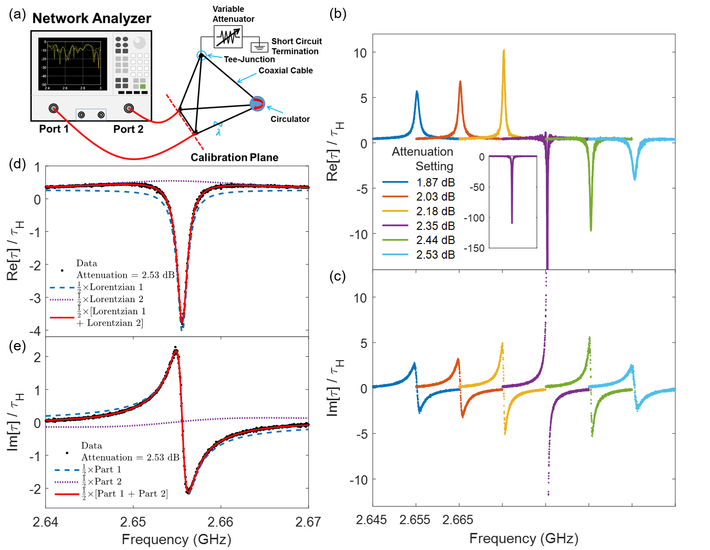
Figure 1: (a) shows a schematic of the graph experimental setup. The lumped loss $\Gamma_{A}$ is varied by changing the applied voltage to the variable attenuator. (b) and (c) show experimental data of both real and imaginary parts of Wigner time delay $\text{Re}[\tau]$ and $\text{Im}[\tau]$ (normalized by the Heisenberg time $\tau_{\text{H}}$) as a function of frequency under different attenuation settings for a single isolated mode. For each attenuation setting, the data is plotted from 2.645 GHz to 2.665 GHz. For clarity, plots with higher attenuation setting are shifted 0.01 GHz from the previous one. Inset shows the entire range of $\text{Re}[\tau]$ for attenuation setting of 2.35 dB. (d) and (e) demonstrate the two-Lorentzian nature of the real and imaginary parts of the Wigner time delay as a function of frequency. The fitting parameters in these two plots are: $\text{Re}z_{n}=2.6556$ GHz, $E_{n}=2.6544$ GHz, $\text{Im}z_{n}-\gamma=-7.1065\times 10^{-4}$ GHz, and $\Gamma_{n}+\gamma=0.0110$ GHz. The constants used in the $\text{Re}[\tau]$ and $\text{Im}[\tau]$ fits are $C_{\text{R}}=0.26$ and $C_{\text{I}}=-0.0018$ in units of $\tau_{\text{H}}$. Detailed discussion about the fitting constants and degree of isolation of the modes can be found in the Supp. Mat. section IV [70].

Experiment. We focus on experiments involving microwave graphs [74, 75, 13, 62] for a number of reasons. First, they provide for complex scattering scenarios with well-isolated modes amenable to detailed analysis. We thus avoid the complications of interacting poles and related interference effects [76]. Graphs also allow for convenient parametric control such as variable lumped lossy elements, variable global loss, and breaking of time-reversal invariance. We utilize an irregular tetrahedral microwave graph formed by coaxial cables and Tee-junctions, having $M=2$ single-mode ports, and broken time-reversal invariance. A voltage-controlled variable attenuator is attached to one internal node of the graph (see Fig. 1(a)), providing for a variable lumped loss ($L=1$, the control variable $\Gamma_{A}$). The nodes involving connections of the graph to the network analyzer, and the graph to the lumped loss, are made up of a pair of Tee-junctions. The coaxial cables and tee-junctions have a roughly uniform and constant attenuation produced by dielectric loss and conductor loss, which is parameterized by the uniform loss parameter $\gamma$. The 2-port graph has a total electrical length of $L_{e}=3.89$ m, a mean mode spacing of $\Delta=c/2L_{e}=38.5$ MHz, and a Heisenberg time $\tau_{\text{H}}=2\pi/\Delta=$ 163 ns. The graph has equal coupling on both ports, characterized by a nominal value of $T_{a}=0.9450$ at a frequency of 2.6556 GHz.

Comparison of Theory and Experiments. Figure 1 shows the evolution of complex time delay for a single isolated mode of the $M=2$ port tetrahedral microwave graph as $\Gamma_{A}$ is varied. The complex time delay is evaluated as in Eq. 5 based on the experimental $S(f)$ data, where $f$ is the microwave frequency, a surrogate for energy $E$. Note that the (calibrated) measured S-parameter data is directly used for calculation of the complex time delay without any data pre-processing. The resulting real and imaginary parts of the time delay vary systematically with frequency, adopting both positive and negative values, depending on frequency and lumped loss in the graph. The full evolution animated over varying lumped loss is available in the Supplemental Material [70]. These variations are well-described by the theory given above.

Figure 1(d) and (e) clearly demonstrates that two Lorentzians are required to correctly describe the frequency dependence of the real part of the time delay. The two Lorentzians have different widths in general, given by the values of $\text{Im}z_{n}-\gamma$ and $\Gamma_{n}+\gamma$, and in this case the Lorentzians also have opposite sign. The frequency dependence of the imaginary part of the time delay also requires two terms, with the same parameters as for the real part, to be correctly described. The data in Fig. 1(b) also reveals that $\text{Re}[\tau]$ goes to very large positive values and suddenly changes sign to large negative values at a critical amount of local loss. For another attenuation setting of the same mode it was found that the maximum delay time was 337 times the Heisenberg time, showing that the signal resides in the scattering system for a substantial time.

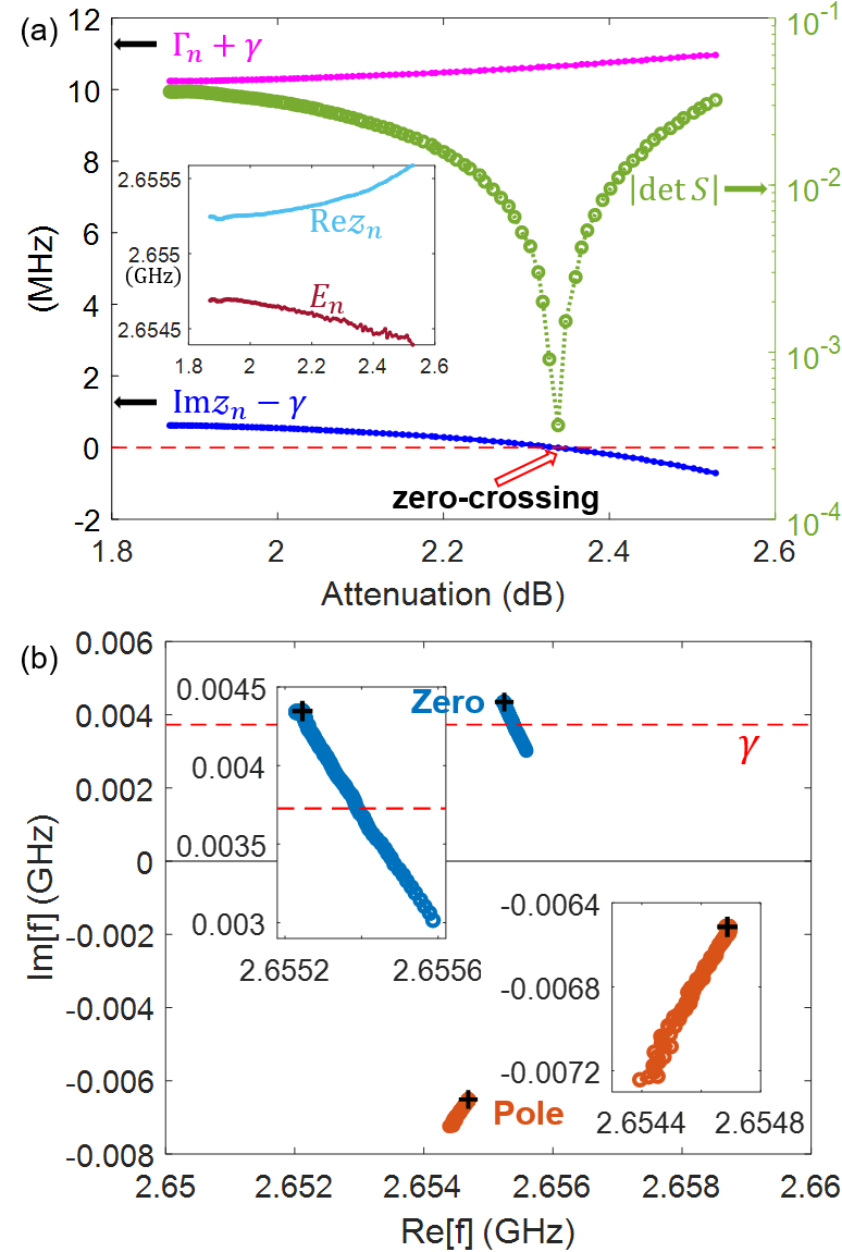
Figure 2: (a) Fitted parameters $\text{Im}z_{n}-\gamma$ and $\Gamma_{n}+\gamma$ for the complex Wigner time delay from graph experimental data. Also shown is the evolution of $|\det(S)|$ at the specific frequency of interest, $f_{\text{CPA}}$, which reaches its minimum at the zero-crossing point. Inset shows the evolution of $\text{Re}z_{n}$ and $E_{n}=\text{Re}\mathcal{E}_{n}$ with attenuation. (b) Evolution of complex zero and pole of a single mode of the graph in the complex frequency plane as a function of $\Gamma_{A}$. The black crosses are the initial state of the zero and pole at the minimum attenuation setting. Insets show the details of the complex zero and pole migrations.

The measured complex time delay as a function of frequency can be fit to Eqs. (7) and (8) to extract the corresponding pole and zero location for the $S$-matrix. The method to perform this fit is described in the Supp. Mat. Section I [70] The fitting parameters are $\text{Re}z_{n}$ and $\text{Im}z_{n}-\gamma$ for the zero, and $E_{n}$ and $\Gamma_{n}+\gamma$ for the pole. Note that the $\text{Re}[\tau(f)]$ and $\text{Im}[\tau(f)]$ data are fit simultaneously, and constant offsets $C_{\text{R}}$ and $C_{\text{I}}$ are added to each fit.

Figure 2 summarizes the parameters required to fit the experimental complex time delay vs. frequency (shown in Fig. 1) as the localized loss due to the variable attenuator in the graph is increased. The significant feature here is the zero-crossing of $\text{Im}z_{n}-\gamma$ at frequency $f=f_{\text{CPA}}$, which corresponds to the point at which $\text{Re}[\tau(f)]$ changes sign. As shown in Fig. 2(a) this coincides with the point at which $|\det(S(f))|$ achieves its minimum value at the CPA frequency $f_{\text{CPA}}$. This demonstrates that one or more eigenvalues of the $S$-matrix go through a complex zero value precisely as the condition $\text{Im}z_{n}-\gamma=0$ and $f-\text{Re}z_{n}=0$ is satisfied. Associated with this condition $|\text{Re}[\tau(f_{\text{CPA}})]|$ diverges, with corresponding large positive and negative values of $\text{Im}[\tau(f)]$ occurring just below and just above $f=f_{\text{CPA}}$. Similar behavior of $\text{Re}[\tau(f)]$ was recently observed in a complex scattering system containing re-configurable metasurfaces, as the pixels were toggled [73].

Next we wish to estimate the value of uniform attenuation $\gamma$ for the microwave graph. Using the unitary deficit of the $S$-matrix in a setup in which the attenuator is removed [17], we evaluate the uniform loss strength $\gamma$ to be $3.73\times 10^{-3}$ GHz (see Supp. Mat. section III [70]).

Figure 2(b) summarizes the locations of the $S$-matrix pole $\mathcal{E}_{n}$ and zero $z_{n}$ of the single isolated mode of the microwave graph in the complex frequency plane as the localized loss is varied. When the $S$-matrix zero crosses the $\text{Im}z_{n}=\gamma$ value, one has the traditional signature of CPA. Note from Fig. 2 that the real parts of the zero and pole do not coincide and in fact move away from each other as localized loss is increased.

Discussion. It should be noted that the occurrence of a negative real part of the time delay is an inevitable consequence of sub-unitary scattering, and is also expected for particles interacting with attractive potentials [78].

The imaginary part of time delay was in the past discussed in relation to changes in scattering unitary deficit with frequency [30]. Another approach to defining complex time delay has been recently suggested to be based on essentially calculating the time delay of the signal which comes out of the system without being absorbed [73]. It should be noted that this ad hoc definition of time delay is not simply related to the poles and zeros of the $S$-matrix. Moreover, a closer inspection shows that such a definition of complex time delay tacitly assumes that the real parts of the pole and zero are identical. According to our theory such an assumption is incompatible with a proper treatment of localized loss.

We emphasize that the correct knowledge of the locations of the poles and zeros is essential for reconstructing the scattering matrix over the entire complex energy plane through Weierstrass factorization [79]. Through graph simulations presented in Sup. Mat. Section VII [70] we demonstrate that the complex time delay theory presented here also works for time-reversal invariant systems, and for systems with variable uniform absorption strength $\gamma$. Our results therefore establish a systematic procedure to find the $S$-matrix zeros and poles of isolated modes of a complex scattering system with an arbitrary number of coupling channels, symmetry class, and arbitrary degrees of both global and localized loss.

Recent work has demonstrated CPA in disordered and complex scattering systems [60, 62]. It has been discovered that one can systematically perturb such systems to induce CPA at an arbitrary frequency [80, 73], and this enables a remarkably sensitive detector paradigm [73]. These ideas can also be applied to optical scattering systems where measurement of the transmission matrix is possible [81]. Here we have uncovered a general formalism in which to understand how CPA can be created in an arbitrary scattering system. In particular this work shows that both the global loss ($\gamma$), localized loss centers, or changes to the spectrum can be independently tuned to achieve the CPA condition.

Future work includes treating the case of overlapping modes, and the development of theoretical predictions for the statistical properties of both the real and imaginary parts of the complex time delay in chaotic and multiple scattering sub-unitary systems.

Conclusions. We have introduced a complex generalization of Wigner time delay which holds for arbitrary uniform/global and localized loss, and directly relates to poles and zeros of the scattering matrix in the complex energy/frequency plane. Based on that we developed theoretical expressions for complex time delay as a function of energy, and found very good agreement with experimental data on a sub-unitary complex scattering system. Time delay and $\det(S)$ share a common feature that CPA and the divergence of $\text{Re}[\tau]$ and $\text{Im}[\tau]$ coincide. This work opens a new window on time delay in lossy systems, enabling extraction of complex zeros and poles of the $S$-matrix from data.

We acknowledge Jen-Hao Yeh for early experimental work on complex time delay. This work was supported by AFOSR COE Grant No. FA9550-15-1-0171, NSF DMR2004386, and ONR Grant No. N000141912481.

References

- Wigner [1955] E. P. Wigner, Lower Limit for the Energy Derivative of the Scattering Phase Shift, Physical Review 98, 145 (1955).
- Smith [1960] F. T. Smith, Lifetime Matrix in Collision Theory, Physical Review 118, 349 (1960).
- Texier [2016] C. Texier, Wigner time delay and related concepts: Application to transport in coherent conductors, Physica E: Low-dimensional Systems and Nanostructures 82, 16 (2016).
- Rotter et al. [2011] S. Rotter, P. Ambichl, and F. Libisch, Generating Particlelike Scattering States in Wave Transport, Physical Review Letters 106, 120602 (2011).
- Carpenter et al. [2015] J. Carpenter, B. J. Eggleton, and J. Schröder, Observation of Eisenbud-–Wigner–-Smith states as principal modes in multimode fibre, Nature Photonics 9, 751 (2015).
- Horodynski et al. [2020] M. Horodynski, M. Kühmayer, A. Brandstötter, K. Pichler, Y. V. Fyodorov, U. Kuhl, and S. Rotter, Optimal wave fields for micromanipulation in complex scattering environments, Nature Photonics 14, 149 (2020).
- Kuipers et al. [2014] J. Kuipers, D. V. Savin, and M. Sieber, Efficient semiclassical approach for time delays, New Journal of Physics 16, 123018 (2014).
- Davy et al. [2015] M. Davy, Z. Shi, J. Wang, X. Cheng, and A. Z. Genack, Transmission Eigenchannels and the Densities of States of Random Media, Physical Review Letters 114, 033901 (2015).
- Fyodorov and Sommers [1997] Y. V. Fyodorov and H.-J. Sommers, Statistics of resonance poles, phase shifts and time delays in quantum chaotic scattering: Random matrix approach for systems with broken time-reversal invariance, Journal of Mathematical Physics 38, 1918 (1997).
- Barra and Gaspard [2001] F. Barra and P. Gaspard, Classical dynamics on graphs, Physical Review E 63, 066215 (2001).
- Stöckmann [1999] H.-J. Stöckmann, Quantum Chaos: An Introduction (Cambridge University Press, 1999).
- Richter [2001] A. Richter, Wave dynamical chaos: An experimental approach in billiards, Physica Scripta T90, 212 (2001).
- Hul et al. [2012] O. Hul, M. Ławniczak, S. Bauch, A. Sawicki, M. Kuś, and L. Sirko, Are Scattering Properties of Graphs Uniquely Connected to Their Shapes?, Physical Review Letters 109, 040402 (2012).
- Kuhl et al. [2013] U. Kuhl, O. Legrand, and F. Mortessagne, Microwave experiments using open chaotic cavities in the realm of the effective Hamiltonian formalism, Fortschritte der Physik 61, 404 (2013).
- Gradoni et al. [2014] G. Gradoni, J.-H. Yeh, B. Xiao, T. M. Antonsen, S. M. Anlage, and E. Ott, Predicting the statistics of wave transport through chaotic cavities by the random coupling model: A review and recent progress, Wave Motion 51, 606 (2014).
- Dietz and Richter [2015] B. Dietz and A. Richter, Quantum and wave dynamical chaos in superconducting microwave billiards, Chaos: An Interdisciplinary Journal of Nonlinear Science 25, 097601 (2015).
- Doron et al. [1990] E. Doron, U. Smilansky, and A. Frenkel, Experimental demonstration of chaotic scattering of microwaves, Physical Review Letters 65, 3072 (1990).
- Genack et al. [1999] A. Z. Genack, P. Sebbah, M. Stoytchev, and B. A. Van Tiggelen, Statistics of wave dynamics in random media, Physical Review Letters 82, 715 (1999).
- Chabanov et al. [2003] A. A. Chabanov, Z. Q. Zhang, and A. Z. Genack, Breakdown of Diffusion in Dynamics of Extended Waves in Mesoscopic Media, Physical Review Letters 90, 203903 (2003).
- Schanze et al. [2005] H. Schanze, H.-J. Stöckmann, M. Martínez-Mares, and C. H. Lewenkopf, Universal transport properties of open microwave cavities with and without time-reversal symmetry, Physical Review E 71, 016223 (2005).
- Kuhl et al. [2008] U. Kuhl, R. Höhmann, J. Main, and H.-J. Stöckmann, Resonance Widths in Open Microwave Cavities Studied by Harmonic Inversion, Physical Review Letters 100, 254101 (2008).
- Di Falco et al. [2012] A. Di Falco, T. F. Krauss, and A. Fratalocchi, Lifetime statistics of quantum chaos studied by a multiscale analysis, Applied Physics Letters 100, 184101 (2012).
- Barkhofen et al. [2013] S. Barkhofen, T. Weich, A. Potzuweit, H.-J. Stöckmann, U. Kuhl, and M. Zworski, Experimental Observation of the Spectral Gap in Microwave -Disk Systems, Physical Review Letters 110, 164102 (2013).
- Gros et al. [2014] J.-B. Gros, U. Kuhl, O. Legrand, F. Mortessagne, E. Richalot, and D. V. Savin, Experimental Width Shift Distribution: A Test of Nonorthogonality for Local and Global Perturbations, Physical Review Letters 113, 224101 (2014).
- Liu et al. [2014] C. Liu, A. Di Falco, and A. Fratalocchi, Dicke Phase Transition with Multiple Superradiant States in Quantum Chaotic Resonators, Physical Review X 4, 021048 (2014).
- Davy and Genack [2018] M. Davy and A. Z. Genack, Selectively exciting quasi-normal modes in open disordered systems, Nature Communications 9, 4714 (2018).
- Fan and Kahn [2005] S. Fan and J. M. Kahn, Principal modes in multimode waveguides, Optics Letters 30, 135 (2005).
- Xiong et al. [2016] W. Xiong, P. Ambichl, Y. Bromberg, B. Redding, S. Rotter, and H. Cao, Spatiotemporal Control of Light Transmission through a Multimode Fiber with Strong Mode Coupling, Physical Review Letters 117, 053901 (2016).
- Gérardin et al. [2016] B. Gérardin, J. Laurent, P. Ambichl, C. Prada, S. Rotter, and A. Aubry, Particlelike wave packets in complex scattering systems, Physical Review B 94, 014209 (2016).
- Böhm et al. [2018] J. Böhm, A. Brandstötter, P. Ambichl, S. Rotter, and U. Kuhl, In situ realization of particlelike scattering states in a microwave cavity, Physical Review A 97, 021801(R) (2018).
- Ambichl et al. [2017] P. Ambichl, A. Brandstötter, J. Böhm, M. Kühmayer, U. Kuhl, and S. Rotter, Focusing inside disordered media with the generalized Wigner–Smith operator, Physical Review Letters 119, 033903 (2017).
- Lehmann et al. [1995] N. Lehmann, D. Savin, V. Sokolov, and H.-J. Sommers, Time delay correlations in chaotic scattering: random matrix approach, Physica D: Nonlinear Phenomena 86, 572 (1995).
- Gopar et al. [1996] V. A. Gopar, P. A. Mello, and M. Büttiker, Mesoscopic Capacitors: A Statistical Analysis, Physical Review Letters 77, 3005 (1996).
- Fyodorov et al. [1997] Y. V. Fyodorov, D. V. Savin, and H.-J. Sommers, Parametric correlations of phase shifts and statistics of time delays in quantum chaotic scattering: Crossover between unitary and orthogonal symmetries, Physical Review E 55, R4857(R) (1997).
- Brouwer et al. [1999] P. W. Brouwer, K. Frahm, and C. W. J. Beenakker, Distribution of the quantum mechanical time-delay matrix for a chaotic cavity, Waves Random Media 9, 91 (1999).
- Savin et al. [2001] D. V. Savin, Y. V. Fyodorov, and H.-J. Sommers, Reducing nonideal to ideal coupling in random matrix description of chaotic scattering: Application to the time-delay problem, Physical Review E 63, 035202(R) (2001).
- Mezzadri and Simm [2013] F. Mezzadri and N. J. Simm, Tau-Function Theory of Chaotic Quantum Transport with = 1, 2, 4, Communications in Mathematical Physics 324, 465 (2013).
- Texier and Majumdar [2013] C. Texier and S. N. Majumdar, Wigner time-delay distribution in chaotic cavities and freezing transition, Physical Review Letters 110, 250602 (2013).
- Novaes [2015] M. Novaes, Statistics of time delay and scattering correlation functions in chaotic systems. I. Random matrix theory, Journal of Mathematical Physics 56, 062110 (2015).
- Cunden [2015] F. D. Cunden, Statistical distribution of the Wigner–Smith time-delay matrix moments for chaotic cavities, Physical Review E 91, 060102(R) (2015).
- Fyodorov et al. [2005] Y. V. Fyodorov, D. V. Savin, and H.-J. Sommers, Scattering, reflection and impedance of waves in chaotic and disordered systems with absorption, Journal of Physics A: Mathematical and General 38, 10731 (2005).
- Beenakker and Brouwer [2001] C. Beenakker and P. Brouwer, Distribution of the reflection eigenvalues of a weakly absorbing chaotic cavity, Physica E: Low-dimensional Systems and Nanostructures 9, 463 (2001).
- Fyodorov [2003] Y. V. Fyodorov, Induced vs. Spontaneous breakdown of S-matrix unitarity: Probability of no return in quantum chaotic and disordered systems, Journal of Experimental and Theoretical Physics Letters 78, 250 (2003).
- Savin and Sommers [2003] D. V. Savin and H.-J. Sommers, Delay times and reflection in chaotic cavities with absorption, Physical Review E 68, 036211 (2003).
- Grabsch [2020] A. Grabsch, Distribution of the Wigner-–Smith time-delay matrix for chaotic cavities with absorption and coupled Coulomb gases, Journal of Physics A: Mathematical and Theoretical 53, 025202 (2020).
- Sokolov and Zelevinsky [1989] V. Sokolov and V. Zelevinsky, Dynamics and statistics of unstable quantum states, Nuclear Physics A 504, 562 (1989).
- Haake et al. [1992] F. Haake, F. Izrailev, N. Lehmann, D. Saher, and H.-J. Sommers, Statistics of complex levels of random matrices for decaying systems, Zeitschrift für Physik B Condensed Matter 88, 359 (1992).
- Fyodorov and Sommers [1996] Y. V. Fyodorov and H. J. Sommers, Statistics of S-matrix poles in few-channel chaotic scattering: Crossover from isolated to overlapping resonances, Journal of Experimental and Theoretical Physics Letters 63, 1026 (1996).
- Fyodorov and Khoruzhenko [1999] Y. V. Fyodorov and B. A. Khoruzhenko, Systematic Analytical Approach to Correlation Functions of Resonances in Quantum Chaotic Scattering, Physical Review Letters 83, 65 (1999).
- Sommers et al. [1999] H.-J. Sommers, Y. V. Fyodorov, and M. Titov, -matrix poles for chaotic quantum systems as eigenvalues of complex symmetric random matrices: from isolated to overlapping resonances, Journal of Physics A: Mathematical and General 32, L77 (1999).
- Fyodorov and Mehlig [2002] Y. V. Fyodorov and B. Mehlig, Statistics of resonances and nonorthogonal eigenfunctions in a model for single-channel chaotic scattering, Physical Review E 66, 045202(R) (2002).
- Poli et al. [2009] C. Poli, D. V. Savin, O. Legrand, and F. Mortessagne, Statistics of resonance states in open chaotic systems: A perturbative approach, Physical Review E 80, 046203 (2009).
- Celardo et al. [2011] G. L. Celardo, N. Auerbach, F. M. Izrailev, and V. G. Zelevinsky, Distribution of Resonance Widths and Dynamics of Continuum Coupling, Physical Review Letters 106, 042501 (2011).
- Fyodorov [2016] Y. V. Fyodorov, Random matrix theory of resonances: An overview, in 2016 URSI International Symposium on Electromagnetic Theory (EMTS), Espoo, Finland (IEEE, 2016) pp. 666–669.
- Li et al. [2017] H. Li, S. Suwunnarat, R. Fleischmann, H. Schanz, and T. Kottos, Random matrix theory approach to chaotic coherent perfect absorbers, Physical Review Letters 118, 044101 (2017).
- Fyodorov et al. [2017] Y. V. Fyodorov, S. Suwunnarat, and T. Kottos, Distribution of zeros of the -matrix of chaotic cavities with localized losses and coherent perfect absorption: non-perturbative results, Journal of Physics A: Mathematical and Theoretical 50, 30LT01 (2017).
- Baranov et al. [2017a] D. G. Baranov, A. Krasnok, and A. Alù, Coherent virtual absorption based on complex zero excitation for ideal light capturing, Optica 4, 1457 (2017a).
- Fyodorov [2019] Y. V. Fyodorov, Reflection Time Difference as a Probe of -Matrix Zeroes in Chaotic Resonance Scattering, Acta Physica Polonica A 136, 785 (2019).
- Krasnok et al. [2019] A. Krasnok, D. Baranov, H. Li, M.-A. Miri, F. Monticone, and A. Alù, Anomalies in light scattering, Advances in Optics and Photonics 11, 892 (2019).
- Pichler et al. [2019] K. Pichler, M. Kühmayer, J. Böhm, A. Brandstötter, P. Ambichl, U. Kuhl, and S. Rotter, Random anti-lasing through coherent perfect absorption in a disordered medium, Nature 567, 351 (2019).
- Osman and Fyodorov [2020] M. Osman and Y. V. Fyodorov, Chaotic scattering with localized losses: -matrix zeros and reflection time difference for systems with broken time-reversal invariance, Physical Review E 102, 012202 (2020).
- Chen et al. [2020] L. Chen, T. Kottos, and S. M. Anlage, Perfect absorption in complex scattering systems with or without hidden symmetries, Nature Communications 11, 5826 (2020).
- F. Imani et al. [2020] M. F. Imani, D. R. Smith, and P. del Hougne, Perfect absorption in a disordered medium with programmable meta-atom inclusions, Advanced Functional Materials 30, 2005310 (2020).
- Mitchell et al. [2010] G. E. Mitchell, A. Richter, and H. A. Weidenmüller, Random matrices and chaos in nuclear physics: Nuclear reactions, Reviews of Modern Physics 82, 2845 (2010).
- Fyodorov and Savin [2011] Y. V. Fyodorov and D. V. Savin, Resonance scattering of waves in chaotic systems, in The Oxford Handbook of Random Matrix Theory, edited by G. Akemann, J. Baik, and P. D. Francesco (Oxford University Press, 2011) pp. 703–722.
- Schomerus [2017] H. Schomerus, Random matrix approaches to open quantum systems, in Stochastic Processes and Random Matrices: Lecture Notes of the Les Houches Summer School 2015, edited by G. Schehr, A. Altland, Y. V. Fyodorov, N. O’Connell, and L. F. Cugliandolo (Oxford University Press, 2017) pp. 409–473.
- Note [1] This way of modelling the localized absorbers as additional scattering channels is close in spirit to the so-called dephasing lead model of decoherence introduced in: M. Büttiker, Role of quantum coherence in series resistors, Phys. Rev. B 33, 3020 (1986) and further developed in P. W. Brouwer and C. W. J. Beenakker, Voltage-probe and imaginary-potential models for dephasing in a chaotic quantum dot, Phys. Rev. B 55, 4695 (1997).
- Rotter [2009] I. Rotter, A non-Hermitian Hamilton operator and the physics of open quantum systems, Journal of Physics A: Mathematical and Theoretical 42, 153001 (2009).
- Lyuboshitz [1977] V. Lyuboshitz, On collision duration in the presence of strong overlapping resonance levels, Physics Letters B 72, 41 (1977).
- [70] See Supplemental Material at [URL will be inserted by publisher] for the details of extracting poles and zeros from data, the sign convention used for the scattering matrix frequency evolution, evaluation of the system uniform loss strength , discussions about effects of neighboring resonances on fitting to the complex time delay, further details about CPA and complex time delay, connections to earlier work on negative real time delay and imaginary time delay, simulations of time-reversal invariant graphs and evaluation of complex time delay with varying uniform loss, and for animations of time delay evolution with variation of lumped loss (experiment Fig. 1 (b) and (c)) or uniform loss (simulation Fig. S4 (b) and (c)).
- Chong et al. [2010] Y. D. Chong, L. Ge, H. Cao, and A. D. Stone, Coherent Perfect Absorbers: Time-Reversed Lasers, Physical Review Letters 105, 053901 (2010).
- Baranov et al. [2017b] D. G. Baranov, A. Krasnok, T. Shegai, A. Alù, and Y. Chong, Coherent perfect absorbers: linear control of light with light, Nature Reviews Materials 2, 17064 (2017b).
- del Hougne et al. [2020] P. del Hougne, K. B. Yeo, P. Besnier, and M. Davy, On-demand coherent perfect absorption in complex scattering systems: time delay divergence and enhanced sensitivity to perturbations (2020), arXiv:2010.06438 [physics.class-ph] .
- Hul et al. [2004] O. Hul, S. Bauch, P. Pakoński, N. Savytskyy, K. Życzkowski, and L. Sirko, Experimental simulation of quantum graphs by microwave networks, Physical Review E 69, 056205 (2004).
- Ławniczak et al. [2008] M. Ławniczak, O. Hul, S. Bauch, P. Seba, and L. Sirko, Experimental and numerical investigation of the reflection coefficient and the distributions of Wigner’s reaction matrix for irregular graphs with absorption, Physical Review E 77, 056210 (2008).
- Persson et al. [1998] E. Persson, K. Pichugin, I. Rotter, and P. Šeba, Interfering resonances in a quantum billiard, Physical Review E 58, 8001 (1998).
- Note [2] The coupling strength is determined by the value of the radiation -matrix (). The radiation is measured when the graph is replaced by loads connected to the three output connectors of each node attached to the network analyzer test cables.
- Smilansky [2017] U. Smilansky, Delay-time distribution in the scattering of time-narrow wave packets. (I), Journal of Physics A: Mathematical and Theoretical 50, 215301 (2017).
- Grigoriev et al. [2013] V. Grigoriev, A. Tahri, S. Varault, B. Rolly, B. Stout, J. Wenger, and N. Bonod, Optimization of resonant effects in nanostructures via Weierstrass factorization, Physical Review A 88, 011803(R) (2013).
- Frazier et al. [2020] B. W. Frazier, T. M. Antonsen, S. M. Anlage, and E. Ott, Wavefront shaping with a tunable metasurface: Creating cold spots and coherent perfect absorption at arbitrary frequencies, Physical Review Research 2, 043422 (2020).
- Popoff et al. [2010] S. M. Popoff, G. Lerosey, R. Carminati, M. Fink, A. C. Boccara, and S. Gigan, Measuring the Transmission Matrix in Optics: An Approach to the Study and Control of Light Propagation in Disordered Media, Physical Review Letters 104, 100601 (2010).