Sulfur Chemistry in the Atmospheres of Warm and Hot Jupiters

Abstract

We present and validate a new network of atmospheric thermo-chemical and photo-chemical sulfur reactions. We use a 1-D chemical kinetics model to investigate these reactions as part of a broader HCNO chemical network in a series of hot and warm Jupiters. We find that temperatures approaching $1400\,\mathrm{K}$ are favourable for the production of H2S and HS around $\mathrm{10^{-3}\,bar}$ at mixing ratios of around $10^{-5}$, an atmospheric level where detection by transit spectroscopy may be possible. At $\mathrm{10^{-3}\,bar}$ and at lower temperatures, down to $1000\,\mathrm{K}$, mixing ratios of S2 can be up to $10^{-5}$, at the expense of H2S and HS, which are depleted down to a mixing ratio of $10^{-7}$. We also investigate how the inclusion of sulfur can manifest in an atmosphere indirectly, by its effect on the abundance of non-sulfur-bearing species. We find that in a model of the atmosphere of HD 209458 b, the inclusion of sulfur can lower the abundance of NH3, CH4 and HCN by up to two orders of magnitude around $\mathrm{10^{-3}\,bar}$. In the atmosphere of the warm Jupiter 51 Eri b, we additionally find the inclusion of sulphur depletes the peak abundance of CO2 by a factor of five, qualitatively consistent with prior models. We note that many of the reactions used in the network have poorly determined rate constants, especially at higher temperatures. To obtain an accurate idea of the impact of sulfur chemistry in hot and warm Jupiter atmospheres, experimental measurements of these reaction rates must take place.

1 Introduction

Sulfur chemistry is known to play an important role in the atmospheric chemistry of planets in our solar system. In Earth’s past, it may have lead to the first Snowball Earth event (Macdonald & Wordsworth 2017), and sulfur isotope ratios can be used as a tracer of Earth’s Great Oxidation Event (Hodgskiss et al. 2019). Sulfur photochemistry is thought to influence the production of hazes and clouds in the upper atmospheres of solar system planets such as Earth (Malin 1997), Venus (Zhang et al. 2012; Titov et al. 2018), Jupiter (Moses et al. 1995) and the moon Io (Irwin 1999). Similar hazes, expected to appear in the atmospheres of exoplanets (He et al. 2020), would greatly affect their observed spectra. This would limit our ability to examine their atmosphere, and make assessments of their habitability challenging (Gao et al. 2017).

Sulfur has also recently been of interest in the field of Jupiter-like exoplanets. A tentative detection of the mercapto radical, HS, in the atmosphere of the hot Jupiter WASP-121 b has been made (Evans et al. 2018). However, it is still uncertain whether HS or another molecule is responsible for the absorption feature seen. The warm Jupiter 51 Eri b has also been an excellent example of the importance of sulfur chemistry. Two groups have produced models of 51 Eri b’s atmosphere, one study did not include sulfur chemistry (Moses et al. 2016) and the other did include sulfur chemistry (Zahnle et al. 2016). Significant differences were found between the two models, in particular in the modelled abundance of CO2, but it was unknown whether this was due to sulfur chemistry or other differences in the models. Thus, we believe that including sulfur chemistry in models of exoplanets, both terrestrial and gas-giant, would be valuable in obtaining more accurate pictures of their atmospheric composition.

There are several works that include sulfur chemistry for exoplanet atmospheres. We highlight a subset of these relevant for the atmospheric chemistry of gas giants. Hu et al. (2013) investigate the photochemistry of H2S and SO2 in terrestrial planet and conclude that their direct detection is unlikely due to rapid photochemical conversion to elemental sulfur and sulfuric acid. Visscher et al. (2006) examine thermo-chemical sulfur chemistry for the hot, deep atmospheres of sub-stellar objects and find H2S to be the dominant sulfur bearing gas. However, due to the high temperatures and pressures of the atmospheres they are studying, disequilibrium effects such as diffusion or photochemistry are not considered. Zahnle et al. (2009) investigate whether sulfur photochemistry could explain the hot stratospheres of hot Jupiters, and find that UV absorption of HS and S2 may provide an explanation. Zahnle et al. (2016) also investigate whether sulfur could form photochemical hazes in the atmosphere of 51 Eri b, and under what conditions they could be formed. They find that sulfur clouds should appear on many planets where UV irradiation is weak. Wang et al. (2017) create synthetic spectra of their hot Jupiter atmospheric models to determine whether H2S and PH3 could be detected by JWST, and find that H2S features should be observable for $\mathrm{T_{eq}}>1500\mathrm{K}$. Gao et al. (2017) examine the effects of sulfur hazes on the reflected light from giant planets and find that the hazes would mask the presence of CH4 and H2O.

We need models to be able to investigate the effects of sulfur on exoplanet atmospheres. One way of modelling the atmosphere of planets is through the use of chemical kinetics models. These exist in the form of 1-D (e.g., Moses et al. 2011; Venot et al. 2012; Rimmer & Helling 2016; Tsai et al. 2017), 2-D (e.g., Agúndez et al. 2014) and 3-D (e.g. Drummond et al. 2018) models. The 1-D models take a network of possible chemical reactions within an atmosphere and a temperature profile of the atmosphere to produce abundance profiles of chemical species. These models are frequently combined with prescriptions for diffusion and include a UV flux applied to the top of the model, to allow a full disequilibrium model to be created. Atmospheric models are obtained by computing these models until they reach a converged steady-state condition.

Throughout the last few decades, chemical models of exoplanetary atmospheres have grown more detailed and complex. What had begun as equilibrium models containing limited molecular species made of only a few elements in small chemical networks (e.g., Lodders & Fegley 2002; Liang et al. 2003; Zahnle et al. 2009) have evolved into large photo-kinetic models containing hundreds of molecular species made of many elements in chemical networks with thousands of reactions (Moses et al. 2011; Venot et al. 2012; Rimmer & Helling 2016). The focus of this work is to continue this evolution. We do so by introducing a new element, sulfur, to the model and to the network described in our previous paper (Hobbs et al. 2019). In this way we can produce a tested and validated network of sulfur chemistry. In this work we apply the network to hot and warm Jupiters. By doing so, we can investigate the importance of sulfur in the atmospheres of exoplanets in both the context of sulfur itself and the way it impacts carbon and oxygen chemistry. It was found in the work of Zahnle et al. (2016) that sulfur photo-chemistry in the atmosphere of the warm Jupiter 51 Eri b was the source of a large number of radicals that went on to catalyse other chemistry. This was a possible explanation for the difference in the CO2 abundance found for 51 Eri b between the sulfur-free models of Moses et al. (2016) and the sulfurous models of Zahnle et al. (2016). We revisit 51 Eri b with our own model, as well as the hot Jupiter HD 209458b, to determine whether we can identify what role sulfur plays in the chemistry of both warm and hot Jupiters.

We begin with a brief overview of the model we’re using. In Section 3 we validate our network for pure thermo-chemical equilibrium and compare our model against the sulfur model of Wang et al. (2017) and Zahnle et al. (2016). Section 4 contains our analysis of the sulfur chemistry occurring in the atmospheres of hot Jupiters, and shows which pathways in our network lead to such chemistry occurring. In Section 5, we examine how sulfur can affect the chemistry of other, non-sulfur species in both warm and hot Jupiters. We discuss our findings and review what we have discovered in Section 6.

2 Model Details

To investigate sulfur chemistry in the atmospheres of hot Jupiters, we chose to use Levi, a one-dimensional photo-kinetics code, originally described in Hobbs et al. (2019). This code was previously developed to model carbon, oxygen and nitrogen chemistry in hot Jupiter atmospheres. It was validated against several other photochemical models of hot Jupiters.

In this work, Levi, is being used to model the atmospheres of Jupiter-like planets. It does so via calculations of:

• The interactions between chemical species

• The effects of vertical mixing due to eddy-diffusion molecular diffusion and thermal diffusion

• Photochemical dissociation due to an incoming UV flux.

And uses the input parameters of:

• The pressure-temperature (P-T) profile of the atmosphere

• The eddy-diffusion ($K_{zz}$) profile of the atmosphere

• The profiles of the UV stellar spectrum

• The metallicity of the atmosphere

• The gravity of the planet.

It uses the assumptions of:

• hydrostatic equilibrium

• The atmosphere being an ideal gas

• The atmosphere is small compared to the planet, such that gravity is constant throughout the atmospheric range being modelled.

By combining all of these factors, abundance profiles of the atmosphere are computed.

As is typical for codes of this type, Levi finds steady-state solutions for species in the atmosphere by solving the coupled one-dimensional continuity equation:

$$\frac{\partial n_{i}}{\partial t}=\mathcal{P}_{i}-\mathcal{L}_{i}-\frac{\partial\Phi_{i}}{\partial z},$$ (1)

where $n_{i}$ (${\mathrm{m}}^{-3}$) is the number density of species $i$, with $i=1,...,N$, with $N$ being the total number of species. $\mathcal{P}_{i}$ (${\mathrm{m}}^{-3}\text{\,}{\mathrm{s}}^{-1}$) and $\mathcal{L}_{i}$ (${\mathrm{m}}^{-3}\text{\,}{\mathrm{s}}^{-1}$) are the production and loss rates of the species $i$. $\partial t$ ($\mathrm{s}$) and $\partial z$ ($\mathrm{m}$) are the infinitesimal time step and altitude step respectively. $\Phi_{i}$ (${\mathrm{m}}^{-2}\text{\,}{\mathrm{s}}^{-1}$) is the upward vertical flux of the species, given by,

$$\Phi_{i}=-(K_{zz}+D_{i})n_{t}\frac{\partial X_{i}}{\partial z}+D_{i}n_{i}\left(\frac{1}{H_{0}}-\frac{1}{H_{i}}-\frac{\alpha_{T,i}}{T}\frac{dT}{dz}\right),$$ (2)

where $X_{i}$ and $n_{t}$ (${\mathrm{m}}^{-3}$) are the mixing ratio and total number density of molecules such that $n_{i}=X_{i}n_{t}$. The eddy-diffusion coefficient, $K_{zz}$ (${\mathrm{m}}^{2}\text{\,}{\mathrm{s}}^{-1}$), approximates the rate of vertical transport and $D_{i}$ (${\mathrm{m}}^{2}\text{\,}{\mathrm{s}}^{-1}$) is the molecular diffusion coefficient of species $i$. $H_{0}$ ($\mathrm{m}$) is the mean scale height, $H_{i}$ ($\mathrm{m}$) is the molecular scale height, $T$ (K) is the temperature, and $\alpha_{T,i}$ is the thermal diffusion factor. For the full explanation of how we determine each of these parameters, and solve the equations, refer to Hobbs et al. (2019).

Previously, we used a subset of the Stand2019 network. This was the STAND2015 network first developed in Rimmer & Helling (2016) plus the additional reactions from Rimmer & Rugheimer (2019). We limited the network to only reactions with neutral species containing hydrogen, carbon, nitrogen and oxygen, and used it in conjunction with Levi to model hot Jupiter atmospheres. As part of this work we have developed a new addition to this network, comprised of an additional 185 reactions and 30 species that include the element sulfur. Our sulfur species include molecules that contain up to 2 H, 3 C, 3 O and 2 S, except for the allotropes of sulfur that include up to S8. These species are tabulated in Table 1. The reactions we have added were mainly drawn from the NIST chemical kinetics database , with the full tabulation of both reactions and sources available in the table of Appendix B.

Table 1: Chemical names of the sulfur species used in the network

Species	Chemical Name
S	Sulfur
S2	Disulfur
S3	Trisulfur
S4	Tetrasulfur
S5	Pentasulfur
S6	Hexasulfur
S7	Heptasulfur
S8	Octasulfur
HS	Mercapto Radical
H2S	Hydrogen Sulfide
H2S2	Hydrogen Disulfide
CS	Carbon Sulfide
CS2	Carbon Disulfide
CS2OH	Thioxomethyl Radical
HCS	Thioformyl Radical
OCS	Carbonyl Sulfide
H2CS	Thioformaldehyde
H2C3S	Tricarbon Monosulfide
CH3SH	Mercaptomethane
HSNO	Thionylimide
SO	Sulfur Monoxide
SO2	Sulfur Dioxide
SO3	Sulfur Trioxide
S2O	Disulfur Monoxide
HSO	Sulfenate
HSO2	Sulfinate
HSO3	Bisulfite
HOSO	Hydroperoxysulfanyl
HSOO	HSOO

We applied a sensible selection criterion when choosing which sources of the rate constants to use for each reaction. Where possible, we selected rate constants that had been measured experimentally, rather than theoretically. This network was intended to be able to apply to hot Jupiters, whose temperatures can reach several thousand Kelvin. As such, we aimed to pick rate constants that had been measured over a range of temperatures, ideally to temperatures that are realistic for a hot Jupiter, i.e., $2000\,\mathrm{K}$. Unfortunately, many reactions have only been measured at room temperature, resulting in currently unavoidable limitations to the accuracy of these rate constants. Finally, we in general picked the more recently measured rate constants, although many have not had new measurements in many decades. In some cases, the rate constants of both the forward and reverse reaction were available. In these cases, we tried to pick the rate constants for the reaction without an energy barrier, and used thermodynamic reversal to obtain the rates for the reverse reaction. We took the estimated rate constants of sulfur allotrope polymerisation from Moses et al. (2002) and several carbon mono-sulphide, CS, reactions from the KIDA database (Wakelam et al. 2012) . These reactions are thermodynamically reversed using the NASA7 polynomials from Burcat , with the full method for these reversals detailed in Hobbs et al. (2019). There are no polynomials for the species CS2OH, H2C3S and HSNO, so we do not reverse the reactions that include these species. We also include the photodissociation cross-sections for 17 reactions involving eleven sulfur species: S2, S3, S4, H2S, SO, SO2, SO3, S2O, OCS, CS2 and CH3SH. The photo-dissociation cross-section, $\Sigma_{i\,\rightarrow\,j}$ ($\mathrm{m^{2}}$) is equal to $\sigma_{a,i}\times q_{a,i\,\rightarrow\,j}$, where $\sigma_{a,i}$ ($\mathrm{m^{2}}$) is the absorption cross-section and $q_{a,i\,\rightarrow\,j}$ is the quantum yield. The wavelengths $i=1\,$ Å  and $j=10000\,$ Å  are the range over which we use these cross-sections. The cross-sections for H2S, SO, SO2, OCS, CS2 and CH3SH were taken from PhIDrates , the cross-sections for S3, S4 and S2 from the MPI-Mainz-UV-VIS Spectral Atlas of Gaseous Molecules and the cross-section for S2 from the Leiden database (Heays et al. 2017).

Here we define which parameters are consistent throughout all models, and what changes are applied to specific models. In all of our models:

• We set the boundary conditions at the top and bottom of the atmosphere to be zero-flux, such that there is no interaction with the atmosphere outside of our model

• When we apply a UV flux to our atmospheres, we choose a mean zenith angle of 57.3^∘ (Zahnle et al. 2008; Hu et al. 2012)

• We model the planet as if its day-side is always facing the star it orbits, i.e. it’s tidally locked, such that it experiences an uninterrupted flux.

Most of our models use a solar metallicity, with values from Asplund et al. (2009). This gives an elemental ratio, as a fraction of the total number of molecules, of: $X_{\ce{H2}}=0.5\times X_{H}=0.8535$, $X_{\ce{He}}=0.145$, $X_{\ce{C}}=4.584\times 10^{-4}$, $X_{\ce{O}}=8.359\times 10^{-4}$, $X_{\ce{N}}=1.154\times 10^{-4}$, $X_{\ce{S}}=2.250\times 10^{-5}$. When we alter the metallicity, we proportionally change the amount of C, O, N and S in the atmosphere. He is kept constant, and H2 is altered such that the ratios sum to unity.

There are also parameters that vary between each model. This includes: the pressure-temperature (P-T) profile, the gravity of the planet, the eddy-diffusion profile applied to the model and the spectral irradiance applied to the top of the atmosphere. An overview of these differences can be seen in Table 2.

Table 2: Model Parameters

Case	Analogue Planet	$T$-profile	Gravity	$K_{zz}$-profile	Metallicity	TOA Spectral Irradiance
		K	cm s-2	cm2 s-1		photons cm-2 s-1 Å-1
Figure 1	Hot Jupiter	1400	1000	None	Solar	None
Figure 2	Hot Jupiter	2000	1000	$10^{9}$	Solar	$800\times$ Solar
Figure 3	WASP-121 b	Evans et al. (2018)	875	$10^{9}$	[M/H] = 1.3	$5300\times$ Solar
Figure 4	Hot Jupiter	Multiple	1000	None	Solar	None
Figure 5	Hot Jupiter	Multiple	1000	$10^{9}$	Solar	$10\times$ Solar
Figure 6	Hot Jupiter	1200	1000	Multiple	Solar	$10\times$ Solar
Figure 7	Hot Jupiter	1200	1000	$10^{9}$	Solar	Multiple
Figure 8	HD 209458 b	Hobbs et al. (2019)	936	Hobbs et al. (2019)	Solar	$800\times$ Solar
Figure 15	51 Eri b	Moses et al. (2016)	3200	$10^{7}$	Solar	Moses et al. (2016)

3 Validation of the Network

In this section we test our model by applying it to the atmospheres of several hot Jupiters. We compare the thermochemistry of our model to an equilibrium solver, FastChem. We also compare and contrast our complete model to a previous sulfur models produced by Wang et al. (2017) and Zahnle et al. (2016).

3.1 Equilibrium Comparison

As a first step of validating our new sulfur network, we chose to consider our results when only allowing thermochemistry, with no disequilibrium chemistry. We compare to the analytical equilibrium output of FastChem, a chemical equilibrium solver produced by Stock et al. (2018). In this comparison, we chose to compare a hot Jupiter atmosphere model with an isothermal temperature of $1400\,\mathrm{K}$. The results of this are shown in Figure 1, where we display only the important sulfur species for comparison. We have a near perfect match compared to the analytic output for every species except for HS, which we slightly under-produce, and OCS, which we slightly over-produce.

We expect the causes for these slight dissimilarities to be due to differences in the thermochemical constants we use to reverse our reaction rates. We use the NASA7 polynomials from Burcat to calculate our Gibbs free energy, while Stock et al. (2018) drew theirs from thermochemical databases, e.g., Chase (1998).

Overall, it can be seen that the thermochemistry of our sulfur network is an excellent match to the analytical solution of FastChem. The slight differences seen between the two models are not large enough to significantly impact the chemistry occurring in the atmosphere. Additionally, at a practical level, the difference seen between the models would not be detectable with present observations.

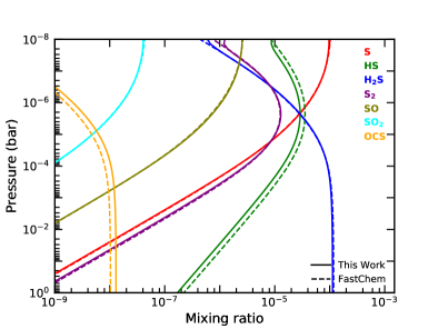
Figure 1: The abundances of significant sulfur bearing species for a purely thermochemical chemistry calculation, taking place in a hot Jupiter atmosphere model that is isothermal at $1400\,\mathrm{K}$, has a gravity of $10\,\mathrm{m\,s^{-2}}$ and a metallicity $5\times$ solar. It has no diffusion or UV spectrum applied to the atmosphere. The solid lines are the output of the model being discussed in this work, while the dashed lines are from the analytical equilibrium solver of FastChem (Stock et al. 2018).

3.2 Comparison with previous sulfur networks

The model of Wang et al. (2017) was used to create synthetic spectra to determine whether JWST could detect sulfur and phosphorous species in the atmosphere of giant planets. We make comparisons between our new network and the output of their model for sulfur species.

In Figure 2, the comparison is made for a hot Jupiter model with an atmosphere at an equilibrium temperature of $1400\,\mathrm{K}$, a $K_{zz}=\mathrm{10^{9}\,cm^{2}\,s^{-1}}$. In this figure, most of the atmosphere shown is dominated by the effects of thermochemistry, with only the very top possibly being effected by the disequilibrium effects of diffusion. We compare the abundances of the seven most abundant sulfur species, S, S2, HS, H2S, SO, OCS and CS.

Throughout the entire atmosphere we see an excellent match between our own model and that of Wang et al. (2017), with the abundance of every species matching very closely between the models. With this, we have firmly validated the thermochemistry of our new sulfur network. Wang et al. (2017) did not include considerations of photochemistry in their model, and so further tests are required to validate the sulfur photochemistry in our model.

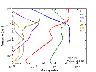
Figure 2: A comparison between our network (solid lines) and one presented in Wang et al. (2017) (dashed lines) for a hot Jupiter model. This atmosphere has an equilibrium temperature of $2000\,\mathrm{K}$, a gravity of $10\,\mathrm{m\,s^{-2}}$, $K_{zz}=\mathrm{10^{9}\,cm^{2}\,s^{-1}}$ and with a solar metalicity.

In Figure 3 we show our model for the hot Jupiter WASP-121 b, and compare to the abundance profile presented in Evans et al. (2018), which was produced by the model of Zahnle et al. (2016). This hot Jupiter is modelled with a metalicity of $20\times$ solar and constant $K_{zz}=\mathrm{10^{9}\,cm^{2}\,s^{-1}}$. The model in Evans et al. (2018) used an F6V host star, whereas here we use a solar host star, with its spectrum scaled as if it were the size and temperature of WASP-121.

We can broadly split the atmosphere in this figure into two regimes. The first is deep in the atmosphere where the pressure is greater than $\mathrm{10^{-3}\,bar}$, and where thermochemical effects are expected to be more important. The second is at pressures less than $\mathrm{10^{-3}\,bar}$ where we expect disequilibrium effects such diffusion and photochemistry to dominate.

In the deep atmosphere, Figure 3 shows that our model has close agreement with the model of Evans et al. (2018), with a difference in predicted abundances of less than 50% between the models. We observe a systematic under-abundance of S-bearing species in our model compared with that of Evans et al. (2018). As the non-S species match closely, this likely reflects a slightly different atmospheric composition being used. More significant differences can be seen in the upper atmosphere, with most of the displayed species varying by several orders of magnitude between the models. We expect this to be primarily due to the difference in the stellar spectrum being applied to this atmosphere. It can be seen in Figure 3 that the general shape of the abundance profiles are very similar, except that our model predicts photochemistry to begin deeper into the atmosphere, a result consistent with the stronger UV spectrum of a G2V star penetrating further. The only other major difference seen in this figure is the profile of S in the upper atmosphere. We believe this to be as a result of differences in how the models treat molecular diffusion.

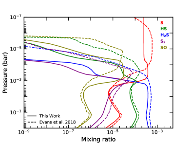
Figure 3: A comparison between our network (solid lines) and the one presented in Evans et al. (2018) (but created by the network of Zahnle et al. (2016)) (dashed lines) for a model of WASP-121 b. The P-T profile for this model is taken from Evans et al. (2018), with constant $K_{zz}=\mathrm{10^{9}\,cm^{2}\,s^{-1}}$, a gravity of $8.75\,\mathrm{m\,s^{-2}}$ and a metalicity $20\times$ solar. The UV spectrum applied to the top of the atmosphere is $5300\times$ Earh’s insolation.

Our new network has also been used in Rimmer et al. (2021) to model sulfur chemistry on Venus. The model in that work produces results very similar to the observations of Venus’s atmosphere, suggesting that the network is valid down to temperatures in the middle atmosphere of Venus; as low as $200\,\mathrm{K}$.

In conclusion, after comparing our new sulfur model against the sulfur models from Wang et al. (2017) and Evans et al. (2018), we see both similarities and differences in the way we treated thermochemistry and photochemistry. We are confident in the accuracy of our thermochemistry after comparisons with the chemical equilibrium solver in Section 3.1. Also, our thermochemical results are very similar to those seen in Evans et al. (2018). Comparing photochemistry is more difficult, but overall the structure of the abundance profiles suggests the photochemistry between this work and Evans et al. (2018) is similar. The discrepancies that can be seen are likely due to differences in UV cross-sections and stellar spectrum.

4 Sulfur in Hot Jupiters

In this section, we investigate sulfur chemistry in the atmosphere of hot Jupiters. We identify the major sulfur species throughout the atmosphere, and note how and why the abundance of these species change. We consider this change in relation to both the planet’s temperature and other properties such as diffusion.

4.1 Local Thermochemical Equilibrium

To begin with, we investigate the simplest scenario for sulfur chemistry in hot Jupiters: An isothermal atmosphere model that is purely in local thermochemical equilibrium, without any form of diffusion or photochemistry.

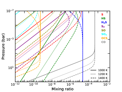
Figure 4: Sulfur chemistry in three isothermal ($1000\mathrm{K}$, $1200\mathrm{K}$ and $1400\mathrm{K}$) hot Jupiter atmospheres in local thermodynamic equilibrium. This atmosphere has a solar metalicity and a gravity of $10\,\mathrm{m\,s^{-2}}$. It has no diffusion or photochemistry applied to it.

In Figure 4 we show comparisons of three isothermal atmospheres in chemical equilibrium. The isothermal temperatures of these atmospheres are $1000\,\mathrm{K}$ (solid), $1200\,\mathrm{K}$ (dotted) and $1400\,\mathrm{K}$ (dashed). All three have a solar metalicity and a gravity of $10\,\mathrm{m\,s^{-2}}$. We plot carbon monoxide, CO, and sulfur bearing species that have a mixing ratio greater than $10^{-10}$ at any point in the atmosphere. In this manner we can show the full scope of sulfur chemistry throughout the entire atmosphere.

The first point of note is the preference of sulfur to form H2S. At all temperatures shown, H2S is the primary carrier of sulfur throughout the majority of the atmosphere, with an abundance of  $2\times 10^{-5}$ for most of the deep atmosphere. It is only at low pressures along the hottest isotherms where this changes, with the primary sulfur carrier becoming atomic S. The reactions that set these abundances are

$${\displaystyle$\, \rightarrow\, $H+HS}$$ (3)

$${\displaystyle$\, \rightarrow\, $H+H2S}$$

$${\displaystyle$\, \rightarrow\, $H2+M}$$

$${\displaystyle$\, \rightarrow\, $H2S}.$$

High temperatures favour the left hand side of this net equation, preferring to dissociate H2S to its constituent H2 and S. In comparison, high pressures favour the formation of H2S from H2 and S. This is why S becomes the most abundant sulfur molecule only at very low pressures along the high temperature isotherms.

The mercapto radical involved in this reaction, HS, is also of interest, as it acts as an intermediary between S and H2S. HS forms a steady pool that quickly reacts to either S or H2S, depending on which is more thermodynamically favoured. Generally, the higher temperature atmospheres favour HS. In all three models, lower pressure increases the abundance of HS. This is unsurprising since, as previously mentioned, the higher temperature and lower pressure favour the dissociation of the large pool of H2S, creating more HS as a result. Although, at the very top of the atmosphere, above $\mathrm{10^{-7}\,bar}$, this changes. Here, the abundance of HS in the $1400\,\mathrm{K}$ atmosphere decreases with pressure and drops below the abundance of HS in the $1200\,\mathrm{K}$ atmosphere. This result arises from atomic S now being the primary sulfur carrier, since its production is favoured by both temperature and pressure. With the majority of sulfur now being in S, the equilibrium abundance of HS decreases.

Both sulfur oxides, SO and SO2, follow similar patterns throughout the atmosphere. They increase in abundance with decreasing pressure, and are more abundant in higher temperature atmospheres. There are two dominant production pathway for SO. At high pressures in the lower temperature atmospheres, the pathway is

$${\displaystyle$\, \rightarrow\, $OH+H+M}$$ (4)

$${\displaystyle$\, \rightarrow\, $H2+HS}$$

$${\displaystyle$\, \rightarrow\, $S+H2}$$

$${\displaystyle$\, \rightarrow\, $H+SO}$$

$${\displaystyle$\, \rightarrow\, $2H2+SO},$$

while in the higher temperature atmosphere, or in any of the modelled atmospheres at low pressures, the pathway is

$${\displaystyle$\, \rightarrow\, $OH+H+M}$$ (5)

$${\displaystyle$\, \rightarrow\, $O+H2}$$

$${\displaystyle$\, \rightarrow\, $H+HSO}$$

$${\displaystyle$\, \rightarrow\, $H+SO}$$

$${\displaystyle$\, \rightarrow\, $H2+M}$$

$${\displaystyle$\, \rightarrow\, $2H2+SO}.$$

In both pathways, the net reaction is unchanged, with the only differences being in the route taken in the pathway.

For SO2 the pathways are

$${\displaystyle$\, \rightarrow\, $OH+H}$$ (6)

$${\displaystyle$\, \rightarrow\, $HOSO}$$

$${\displaystyle$\, \rightarrow\, $SO2+H}$$

$${\displaystyle$\, \rightarrow\, $H2+M}$$

$${\displaystyle$\, \rightarrow\, $SO2+H2},$$

for the deep atmosphere, or more directly

$${\displaystyle$\, \rightarrow\, $OH+H2}$$ (7)

$${\displaystyle$\, \rightarrow\, $SO2+H}$$

$${\displaystyle$\, \rightarrow\, $SO2+H2},$$

for the upper atmosphere.

The sulfur molecules HSO and HOSO referenced in these pathways are not shown in Figure 4 due to their very low abundance. The production of both SO and SO2 starts with the destruction of H2S by an oxygen radical, O. This produces the short lived species HSO that quickly dissociates into SO. SO subsequently reacts with the hydroxyl radical, OH. At pressures greater than $\mathrm{10^{-1}\,bar}$, this reaction forms the very short lived species HOSO, that then dissociates into SO2. At pressures less than $\mathrm{10^{-1}\,bar}$, SO and OH react directly to form SO2. The production of SO is significantly faster than the reaction rate of SO with OH. As a result, the equilibrium abundance of SO is much larger than that of SO2. Near the top of the atmosphere, above $\mathrm{10^{-6}\,bar}$ in the $1400\,\mathrm{K}$ isothermal atmosphere, the abundances of SO and SO2 stop increasing with decreasing pressure. This happens due to the H2S abundance dropping. It is now no longer as available to start the production pathway of SO and SO2.

The pathway producing the sulfur molecule OCS is

$${\displaystyle$\, \rightarrow\, $HS+H2}$$ (8)

$${\displaystyle$\, \rightarrow\, $OCS+H}$$

$${\displaystyle$\, \rightarrow\, $OCS+H2}.$$

In the deep atmosphere, below $\mathrm{10^{-1}\,bar}$, the abundance of OCS is controlled by the abundance of CO. Above this pressure, there is a zone for which both H2S and CO have a constant abundance. This leads OCS to stay at a constant abundance at these pressures. Above $\mathrm{10^{-4}\,bar}$ for the $1400\,\mathrm{K}$ atmosphere, and $\mathrm{10^{-6}\,bar}$ for the $1200\,\mathrm{K}$ atmosphere, the drop in the abundance of H2S results in the mixing ratio of OCS decreasing at a similar rate.

The allotrope of sulfur, S2, is produced by the pathway

$${\displaystyle$\, \rightarrow\, $HS+H2}$$ (9)

$${\displaystyle$\, \rightarrow\, $S2+H}$$

$${\displaystyle$\, \rightarrow\, $S2+H2}.$$

Thus, the abundance of S2 is controlled by the abundance of S and HS (and therefore H2S). This results in a general increase of abundance as pressure decreases. The exception is for the case of the $1400\,\mathrm{K}$ isotherm, where the drop in abundance of H2S and HS above $\mathrm{10^{-6}\,bar}$ leads to a decrease in the mixing ratio of S2.

4.2 Disequilibrium

The atmospheres of most planets are not in chemical equilibrium at low pressure (< $\mathrm{10^{-3}\,bar}$). Therefore it is important to consider how the disequilibrium effects of diffusion and photochemistry can impact the expected sulfur chemistry in a planet’s atmosphere. The lowest pressure shown for our disequilibrium figures is $\mathrm{10^{-7}\,bar}$. This is theoretically high enough in the atmosphere that sulfur-ionizing photons could form an ionosphere. The consideration of ion-chemistry is outside the scope of this work, but it is important to note that the top of our modelled atmospheres do not include this effect.

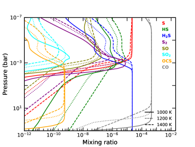
Figure 5: Sulfur chemistry in three isothermal ($1000\mathrm{K}$, $1200\mathrm{K}$ and $1400\mathrm{K}$) hot Jupiter atmospheres in steady-state. This atmosphere has a solar metalicity, a gravity of $10\,\mathrm{m\,s^{-2}}$, constant $K_{zz}=\mathrm{10^{9}\,cm^{2}\,s^{-1}}$ and a UV flux $10\times$ Earth’s.

In Figure 5 we show the same three isothermal atmospheres as in the previous section: Isotherms of $1000\,\mathrm{K}$ (Solid), $1200\,\mathrm{K}$ (Dotted) and $1400\,\mathrm{K}$ (Dashed). Once again, all three have a solar metalicity and a gravity of $10\,\mathrm{m\,s^{-2}}$. All of these atmospheres now have a constant eddy diffusion $K_{zz}=\mathrm{10^{9}\,cm^{2}\,s^{-1}}$. They also have a UV spectrum applied to the top of the atmosphere of $10\times$ Earth’s received solar flux.

In the deep atmosphere, below about $\mathrm{10^{-1}\,bar}$, the abundances are near identical to the equilibrium results presented in the previous section. At this depth, the high pressure ensures that the reaction rates are fast enough that the disequilibrium effects of diffusion and photo-dissociation do not have a significant impact on the chemistry previously presented.

Higher in the atmosphere, above $\mathrm{10^{-3}\,bar}$, we start to see the significance of disequilibrium chemistry. Many of the sulfur molecules are susceptible to photo-dissociation.

Once again H2S is of particular note. At $\mathrm{10^{-3}\,bar}$ it is rapidly dissociated by free H radicals that are produced by photolysis, and then diffuse down from higher in the atmosphere

$$\ce{H2O+}h\nu\ce{&$\, \rightarrow\, $OH+H}$$ (10)

$${\displaystyle$\, \rightarrow\, $H2O+H}$$

$${\displaystyle$\, \rightarrow\, $HS+H2}$$

$${\displaystyle$\, \rightarrow\, $S+H2}$$

$${\displaystyle$\, \rightarrow\, $S+H2}.$$

This effect occurs at all temperatures. Although, in the colder models, we see the abundance of H2S driven much further away from its equilibrium value, by more than two orders of magnitude, compared to the hotter models. This is because of the longer chemical timescales at lower temperatures, which slows the recombination reactions. Overall, the rapid destruction of H2S allows for full dissociation to atomic S. This results in S being the primary sulfur molecule at all temperatures and pressures above $\mathrm{10^{-3}\,bar}$.

The production of a large available pool of S has knock-on effects for the abundance of SO and SO2. Above $\mathrm{10^{-3}\,bar}$ the abundance of SO is controlled by the reaction chain of

$$\ce{SO+}h\nu\ce{&$\, \rightarrow\, $S+O}$$ (11)

$$\ce{H2O+}h\nu\ce{&$\, \rightarrow\, $OH+H}$$

$${\displaystyle$\, \rightarrow\, $SO+H}$$

$${\displaystyle$\, \rightarrow\, $H2+M}$$

$${\displaystyle$\, \rightarrow\, $H2+O},$$

and SO2 by a very similar chain

$$\ce{SO2+}h\nu\ce{&$\, \rightarrow\, $SO+O}$$ (12)

$$\ce{H2O+}h\nu\ce{&$\, \rightarrow\, $OH+H}$$

$${\displaystyle$\, \rightarrow\, $SO2+H}$$

$${\displaystyle$\, \rightarrow\, $H2+M}$$

$${\displaystyle$\, \rightarrow\, $H2+O}.$$

Overall, both these reaction pathways act as a dissipative cycle that increases the abundance of atomic O in the atmosphere, while preventing SO and SO2 from being permanently dissociated. The abundances of both SO and SO2 are primarily determined by the amount of atomic S in the atmosphere. As a result the abundances of SO and SO2 are nearly temperature independent throughout the upper atmosphere: SO reaches abundances around $\mathrm{10^{-7}}$, while SO2 is never greater than $\mathrm{10^{-9}}$.

S2 is significantly affected by the introduction of disequilibrium chemistry. The large increase in both HS and S around $\mathrm{10^{-3}\,bar}$ greatly boosts its production through the reaction

$${\displaystyle$\, \rightarrow\, $S2+H}.$$ (13)

This is particularly prominent in the lower temperature isotherms. In the $1000\,\mathrm{K}$ atmosphere, the abundance of S2 reaches nearly $\mathrm{10^{-5}}$ (compared to only $\mathrm{10^{-10}}$ at the same pressure and temperature in the local thermochemical equilibrium case). However, above $\mathrm{10^{-3}\,bar}$, it is rapidly photo-dissociated into 2S. The outcome is a quick drop-off in its abundance at all temperatures.

OCS is not greatly affected by the introduction of disequilibrium chemistry. Its abundance is still determined by the pathway shown in equation 8.

4.3 Diffusion Strength

It is important to understand how our choices for the parameters of the disequilibrium chemistry can affect the overall distribution of sulfur chemistry in planetary atmospheres. To that end, in Figure 6, we compare three atmospheric models of a $1200\,\mathrm{K}$ isothermal hot Jupiter with different strengths of eddy-diffusion, $K_{zz}$. We do so to test the sensitivity of sulfur chemistry to the strength of the vertical mixing in the atmosphere. We chose to use two extremes of diffusion, $K_{zz}=\mathrm{10^{6}\,cm^{2}\,s^{-1}}$ (Dashed) and $K_{zz}=\mathrm{10^{12}\,cm^{2}\,s^{-1}}$ (Solid), to understand the limiting cases for diffusion. We also include the previously used average case of $K_{zz}=\mathrm{10^{9}\,cm^{2}\,s^{-1}}$ (Dotted) as a comparison.

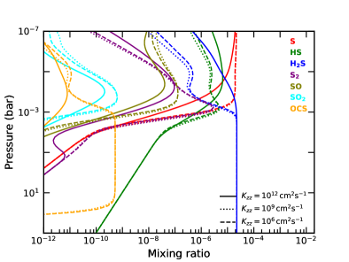
Figure 6: Sulfur chemistry in a $1200\,\mathrm{K}$ isothermal hot Jupiter atmosphere. This model explores the sensitivity of sulfur chemistry to the strength of the vertical mixing, by comparing models with three different $K_{zz}$ values. This atmosphere has a solar metalicity, a gravity of $10\,\mathrm{m\,s^{-2}}$ and has a UV spectrum $10\times$ Earth’s applied to it.

Immediately seen is that the weakest mixing, $K_{zz}=\mathrm{10^{6}\,cm^{2}\,s^{-1}}$, does not differ greatly from the intermediate case of $K_{zz}=\mathrm{10^{9}\,cm^{2}\,s^{-1}}$. This suggests that $K_{zz}=\mathrm{10^{9}\,cm^{2}\,s^{-1}}$ is already sufficiently low that eddy-diffusion is having little effect upon sulfur chemistry.

For the strongest diffusion, $K_{zz}=\mathrm{10^{12}\,cm^{2}\,s^{-1}}$, there are several significant differences to the abundance of sulfur molecules. Most of these effects stem from the diffusion quenching the H2S, such that it stays as the most abundant sulfur molecule up until $\mathrm{10^{-5}\,bar}$. This results in a lower atomic S abundance, which has a knock-on effect of also lowering the abundance of both SO and SO2.

The sulfur allotrope S2 is also significantly affected by the stronger diffusion. Its abundance between $\mathrm{10^{-1}\,bar}$ and $\mathrm{10^{-4}\,bar}$ drops by up to two orders of magnitude compared to the weaker diffusion cases. This is largely caused by the S2 diffusing higher into the atmosphere where it can be photo-dissociated, which causes the drop-off in abundance from $\mathrm{10^{-1}\,bar}$. Above $\mathrm{10^{-4}\,bar}$, the stronger diffusion lifts the abundance of S2 faster than it can be dissociated, to mixing ratios slightly above that of the weaker diffusion models.

Overall, the strength of the vertical mixing does not have much impact on most sulfur molecules. This conclusion is in line with previous studies by Zahnle et al. (2009) and Zahnle et al. (2016), in which they found that vertical mixing was only significant in lower temperatures due to how fast sulfur reactions are. The atmospheres being studied in this work are sufficiently hot that the atmosphere reaches a steady-state balance between the thermo-chemical and photo-chemical elements. The effects of diffusion are thus negated unless the value of $K_{zz}$ is increased to extreme values. At these extremes, the strong mixing may be able to keep H2S detectable higher in the atmosphere, but strong mixing also significantly suppresses the abundance of S2, preventing its abundance from reaching detectable levels.

4.4 UV Strength

We next examine how altering the strength of the UV flux being applied to the top of the model can alter the sulfur chemistry. While this is not a very realistic change to be made independent of all other parameters, (since the flux strength is most commonly set by the distance of the planet from the star, which would greatly impact the atmosphere’s temperature), it is important to understand our network’s sensitivity to changes in the rate of photochemistry. As such, we present three different models of a hot Jupiter with a $1200\,\mathrm{K}$ isothermal atmosphere in Figure 7. Two have extremes of UV irradiation at $100\times$ Earth’s (Solid) and $1\times$ Earth’s (Dashed). The other has $10\times$ Earth’s (Dotted) irradiation, the same as previously used in this section.

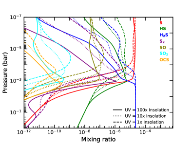
Figure 7: Sulfur chemistry in a $1200\,\mathrm{K}$ isothermal hot Jupiter atmosphere. This model explores the sensitivity of sulfur chemistry to the strength of the UV flux, by comparing models with three different strength of UV. This atmosphere has a solar metalicity, $K_{zz}=\mathrm{10^{9}\,cm^{2}\,s^{-1}}$ and a gravity of $10\,\mathrm{m\,s^{-2}}$.

Most species show no change deep in the atmosphere, below the $\mathrm{10^{-2}\,bar}$ level. No species show any difference below $\mathrm{10^{-1}\,bar}$. This shows that even for extreme irradiation, the deepest parts of the atmosphere are difficult to move away from thermochemical equilibrium.

The species primarily affected by the change in UV flux is H2S. Its abundance drops by an order of magnitude at $\mathrm{10^{-3}\,bar}$ for the highest flux compared to the lowest flux. This also greatly impacts the S at the same pressure. Its abundance is up to five orders of magnitude greater for the greatest flux compared to the smallest. This difference is only seen for a small pressure window however, and the abundance of S is very similar across all three fluxes above $\mathrm{10^{-4}\,bar}$.

In this same pressure window, the greater availability of S caused by the stronger flux allows the abundance of both SO and SO2 to grow much larger than in the models with weaker fluxes. However, above $\mathrm{10^{-4}\,bar}$ this is reversed as the available S becomes similar in all three models, resulting in the strongest UV model depleting SO and SO2 by about an order of magnitude compared to the weakest UV model.

The comparative abundance of S2 goes through several phases. Deep in the atmosphere, around $\mathrm{10^{-1}\,bar}$, the stronger UV flux can penetrate deep enough to begin to dissociate it into 2S. However, not far above this, around $\mathrm{10^{-2}\,bar}$, the excess S that are produced by H2S dissociation in the stronger UV cases are sufficient to boost the production of S2 above its rate of photo-dissociation. Thus we see more S2 in the stronger UV model, up until between $\mathrm{10^{-3}\,bar}$ and $\mathrm{10^{-4}\,bar}$ when the availability of atomic S equalises across all three models. Above this, the stronger UV flux once again dominates in dissociating S2, resulting in its abundance being several orders of magnitude lower than in the weak UV model.

Overall, the strength of the UV flux simply shifts the abundance profiles deeper into the atmosphere. This happens because the stronger flux can penetrate deeper, with an increase of two orders of magnitude in UV flux able to push the profiles of sulfur molecules one order of magnitude deeper in pressure into the atmosphere.

5 The impact of Sulfur’s inclusion on atmospheric chemistry

In this section we investigate what effect the sulfur chemistry has upon the modelled composition of both the hot Jupiter HD 209458b and the warm Jupiter 51 Eri b. We compare atmospheric models of these planets with and without sulfur included in our network. In this way we isolate sulfur’s impact, and examine the pathways in our network that lead to these chemical differences occurring.

5.1 HD 209458 b

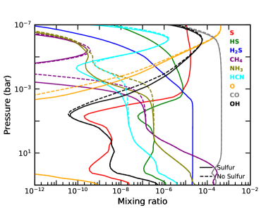
Figure 8: A comparison of the abundance profiles for the hot Jupiter HD 209458b both with (solid lines) and without (dashed lines) our new sulfur network being included. This model uses the pressure - temperature profile and $K_{zz}$ profile from Hobbs et al. (2019). It has solar metalicity, a gravity of $9.36\,\mathrm{m\,s^{-2}}$ and has a UV spectrum $800\times$ Earth’s applied to it.

We chose to examine the effects of sulfur chemistry on the atmosphere of the well studied hot Jupiter, HD 209458b. We have previously investigated this planet with Levi in Hobbs et al. (2019), and we return to it again. We do so now with our updated chemical model to discover how the inclusion of sulfur chemistry affects the predicted abundance profiles of this hot Jupiter’s atmosphere.

As can be seen in Figure 8, we see no difference due to the inclusion of sulfur below 1 bar, in the deep atmosphere of the planet. At this depth, the abundance of the main sulfur species is set by the same reaction path as shown in Reaction LABEL:reac:Smain. These reactions are very rapid and interactions with other species are slow by comparison, preventing sulfur from having any effect on CNO chemistry in the deep atmosphere.

Higher in the atmosphere, around $\mathrm{10^{-3}\,bar}$, sulfur has a much more significant effect on the CNO chemistry. In Figure 8, it can be seen that at this pressure the inclusion of sulfur decreases the predicted abundance of NH3, CH4 and HCN by up to two orders of magnitude.

Through a thorough and careful analysis of the fastest reaction pathways that cause the destruction of NH3, CH4 and HCN, we can identify how and why sulfur causes these differences. Figure 8 shows that sulfur chemistry changes where these three molecules stop being quenched. Molecules stop being quenched when the chemical timescale of the rate limiting step in the fastest destruction pathway becomes faster than the dynamical timescale in that region of the atmosphere. By examining this region for NH3, CH4 and HCN, and how it changes location with the inclusion of sulfur, can determine why sulfur chemistry effects the abundance of CNO species within the atmosphere of a hot Jupiter. We use the chemical timescale as

$$\tau_{chem}=\frac{[X]}{d[X]/dt},$$ (14)

where $[X]$ is the number density of the molecule we are investigating, either NH3, CH4 or HCN. $d[X]/dt$ is the change in number density of $X$ with time, which is approximately the reaction rate of the rate limiting step in the fastest destruction pathway of $[X]$. We treat the dynamic timescale as

$$\tau_{dyn}=\frac{H_{0}dH}{K_{zz}},$$ (15)

where $H_{0}$ is the scale height of the atmosphere, $dH$ is the thickness of one atmospheric layer in our model, and $K_{zz}$ is the eddy-diffusion (Visscher & Moses 2011).

The most efficient pathway for the destruction of NH3 leads the nitrogen to end up in the stable molecule N2, via the following scheme:

$${\displaystyle$\, \rightarrow\, $NH2+H2)}$$ (16)

$${\displaystyle$\, \rightarrow\, $NH+H2)}$$

$${\displaystyle$\, \rightarrow\, $N+H2}$$

$${\displaystyle$\, \rightarrow\, $HNO+H2}$$

$${\displaystyle$\, \rightarrow\, $NO+H2}$$

$$\boldsymbol{\ce{NO+N}} \boldsymbol{\ce{$\, \rightarrow\, $N2+O}}$$

$${\displaystyle$\, \rightarrow\, $OH+H}$$

$${\displaystyle$\, \rightarrow\, $H2O+H}$$

$${\displaystyle$\, \rightarrow\, $H+H+M)}$$

$${\displaystyle$\, \rightarrow\, $N2+3H2},$$

with the reaction in bold being the rate limiting step in the pathway. We show the chemical timescales of each of the main steps in this pathway in Figure 9, as well as the dynamic timescale, all as a function of pressure. We compare these rates for both an atmosphere including sulfur and a sulfur free atmosphere. When we examine where $\tau_{chem}$ of the rate limiting step, NO + N $\,\rightarrow\,$ N2 + O, becomes shorter than $\tau_{dyn}$, we see a significant pressure difference between the sulfur and sulfur-free cases being examined. This pressure difference matches up precisely to where we see NH3 quenching end in Figure 8; around $\mathrm{10^{-3}\,bar}$ with sulfur, and $\mathrm{3x10^{-4}\,bar}$ without sulfur.

The presence of NO in the rate limiting step is why the inclusion of sulfur significantly effects its timescale. Figure 9 also includes the timescale of NO photodissociation, and it can be seen that the presence of sulfur increases the timescale of this reaction by many orders of magnitude between $\mathrm{10^{-3}}$ and $\mathrm{10^{-2}\,bar}$. This large slowing in the destruction of NO results in significantly more NO available in the atmosphere, greatly increasing the rate of the rate limiting step, resulting in the difference in the location of the end of quenching between the two models, and the lower abundance of NH3 seen in the sulfurous model of HD 209458b.

The difference in the photochemical rate of NO arises from the UV shielding by sulfur molecules. In particular, we find that H2S is responsible for most of the additional UV shielding when sulfur is introduced to the atmosphere. This can be seen in Figure 10 where we show the UV flux at different pressure levels, and compare to the same atmosphere but with transparent H2S. We find that H2S causes the available flux around $\mathrm{10^{-3}\,bar}$ to drop by tens of orders of magnitude, depending on the wavelengths being examined. Thus H2S blocks a large fraction of the incoming UV light, allowing NO to survive until higher in the atmosphere compared to a sulfur free atmosphere.

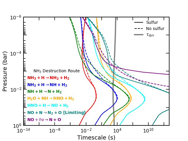
Figure 9: A comparison of the chemical timescales in the most efficient pathway to destroy NH3 in the atmosphere of HD 209458b, for both an sulfurous and a sulfur-free atmosphere. The dynamic timescale is also shown in this figure. The pressure at which the rate limiting step occurs on a shorter timescale than the dynamic timescale is where we expect to see quenching of NH3 end in the atmosphere of HD 209458b. The increase in the timescale of the photodissociation of NO with the inclusion of sulfur is responsible for the difference in where the rate limiting drops below the dynamic timescale.

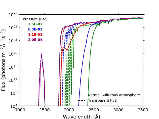
Figure 10: The apparent flux at different pressures within the atmosphere of a sulfurous HD 209458b. To show the effect of sulfur shielding in this atmosphere, we compare the normal flux to the flux if H2S was transparent.

When we examine the dominant destruction pathway for CH4, we find that the carbon tends to end up in CO via;

$${\displaystyle$\, \rightarrow\, $CH3+H2}$$ (17)

$$\boldsymbol{\ce{CH3+OH}} \boldsymbol{\ce{$\, \rightarrow\, $CH2O+H2}}$$

$${\displaystyle$\, \rightarrow\, $CHO+H)}$$

$${\displaystyle$\, \rightarrow\, $CO+H2}$$

$${\displaystyle$\, \rightarrow\, $OH+H2}$$

$${\displaystyle$\, \rightarrow\, $H+H+M)}$$

$${\displaystyle$\, \rightarrow\, $CO+3H2},$$

with the bold reaction once again being the rate limiting step in the this reaction pathway. We show the main timescales of this reaction pathway in Figure 12. Once again we see the rate limiting step’s timescale become smaller than the dynamic timescale at different pressures in a sulfurous vs. a non-sulfurous atmosphere. The explanation for this lies within a different set of reactions:

$$\ce{SO+}\ h\nu\ce{&$\, \rightarrow\, $S+O}$$ (18)

$${\displaystyle$\, \rightarrow\, $OH+H}$$

$${\displaystyle$\, \rightarrow\, $SO+H}.$$

In a sulfurous atmosphere, the photodissociation of SO produces O significantly faster than any other reaction between $\mathrm{10^{-3}}$ and $\mathrm{10^{-4}\,bar}$. This results in a corresponding rate increase in the reaction O + H2   →  OH + H. The timescales of both of these reactions are also shown in Figure 12. The result of these rate increases can be seen in Figure 8, where both O and OH have their abundances increased by at least an order of magnitude around $\mathrm{10^{-3}\,bar}$. The rate limiting step in the destruction of CH4 is dependant on the OH abundance. Thus, the consequence of an increase in OH abundance is that the timescale of the rate limiting step in a sulfurous atmosphere becomes shorter than the dynamic timescale deeper in the atmosphere. This leads to the quenching of CH4 ending deeper in the atmosphere, and the difference in abundance between sulfurous and non-sulfurous atmosphere, as seen in Figure 8.

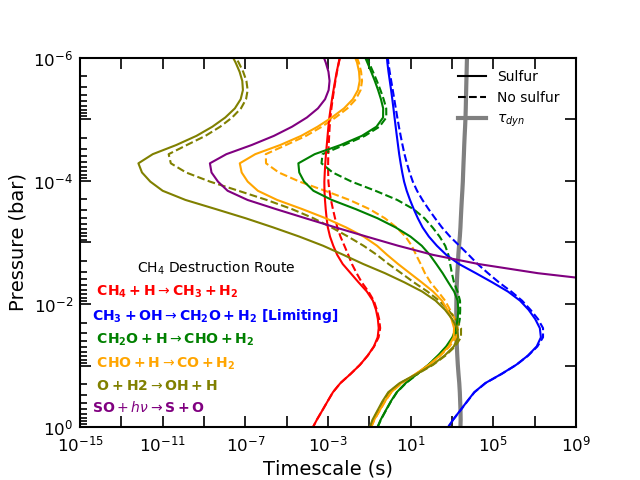
Figure 11: A comparison of the chemical timescales in the most efficient pathway to destroy CH4 in the atmosphere of HD 209458b, for both an sulfurous and a sulfur-free atmosphere. The dynamic timescale is also shown in this figure. The pressure at which the rate limiting step occurs on a shorter timescale than the dynamic timescale is where we expect to see quenching of CH4 end in the atmosphere of HD 209458b. The photodissociation of SO causes a 30x increase in available O, which greatly increases the rate that O becomes OH, and thus is responsible for the change in the rate limiting step of this reaction pathway.

We have found the most efficient pathway for the destruction of HCN to be via the route:

$${\displaystyle$\, \rightarrow\, $HNC+M}$$ (19)

$$\boldsymbol{\ce{HNC+OH}} \boldsymbol{\ce{$\, \rightarrow\, $HNCO+H}}$$

$${\displaystyle$\, \rightarrow\, $CO+NH2}$$

$${\displaystyle$\, \rightarrow\, $NH3+H}$$

$${\displaystyle$\, \rightarrow\, $OH+H2}$$

$${\displaystyle$\, \rightarrow\, $CO+NH3},$$

with the rate limiting step in bold. The explanation for the difference in abundance of HCN in sulfurous and non-sulfurous atmospheres follows the same reasoning as for CH4. Once again, the rate limiting step contains OH, and thus Reactions 18 explain why the inclusion of sulfur increases the abundance of OH, and thus the increase the rate at which HCN is destroyed.

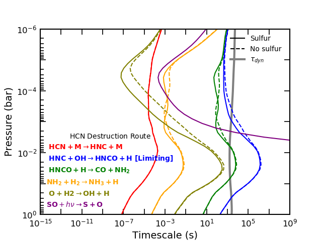
Figure 12: A comparison of the chemical timescales in the most efficient pathway to destroy HCN in the atmosphere of HD 209458b, for both an sulfurous and a sulfur-free atmosphere. The dynamic timescale is also shown in this figure. The pressure at which the rate limiting step occurs on a shorter timescale than the dynamic timescale is where we expect to see quenching of HCN end in the atmosphere of HD 209458b. The photodissociation of SO causes a 30x increase in available O, which greatly increases the rate that O becomes OH, and thus is responsible for the change in the rate limiting step of this reaction pathway.

Overall, the change in the abundance of both HCN and CH4 with the inclusion of sulfur show the catalytic role that sulfur chemistry can have in planetary atmospheres (as also noted by Zahnle et al. 2016)

Figure 8 shows that, at pressures lower than $\mathrm{10^{-5}\,bar}$, the effects of sulfur once again become insignificant. Above this height, H2S begins to drop in abundance, making the shielding of NO less effective. This results in the sulfurous and non-sulfurous photodissociation rates of NO approach similar rates once more, such that the overall destruction rate of NH3 is now approximately the same in both models. Additionally, above this height, SO is no longer the fastest producer of O, with other reactions such as OH photodissociation becoming more dominant. As such, both sulfurous and non-sulfurous destruction rates of CH4 and HCN become similar. In consequence, the very upper atmospheres of hot Jupiters that contain sulfur look nearly indistinguishable from those without sulfur.

There is potential for detecting the differences caused by the inclusion of sulfur in hot Jupiters’ atmospheres. There has already been evidence for CH4 (Guilluy et al. 2019) and HCN (Hawker et al. 2018; Cabot et al. 2019) detections in the atmosphere’s of hot Jupiters. Most retrievals identify species, and their abundances, around the pressure of $\mathrm{10^{-3}\,bar}$. Thus, it should be possible to detect the drop in abundance of these molecules due to sulfur. However, the pressure range over which there is an identifiable difference due to sulfur is rather limited. Any investigated spectra of this planet would need to be very precise, more so than any currently obtainable.

5.2 Warm Jupiters

Previously, there has been discussion in the literature about how sulfur on warm Jupiters may affect the abundance of species in the atmosphere of these planets. Of particular note is the warm Jupiter 51 Eri b, which both Moses et al. (2016) and Zahnle et al. (2016) have modelled in the past. Moses et al. (2016) ran models without any sulfur in the atmosphere, while Zahnle et al. (2016) ran models with sulfur. Both works studied the chemistry of 51 Eri b in great detail, both with and without sulfur. What is of particular interest though are the differences found between the two models. As Moses et al. (2016) notes, they find up to two orders of magnitude more CO2 than Zahnle et al. (2016) for otherwise identical conditions. Thus, our focus in this section will be on examining the warm Jupiter 51 Eri b with both our sulfurous and non-sulfurous models to determine if sulfur is responsible for this difference, and, if it is, why.

To begin this section, we directly compare our model for the atmosphere of 51 Eri b to that of Moses et al. (2016) and Zahnle et al. (2016) as a benchmark for whether differences in the models themselves could be responsible for the difference in CO2 abundance. In Figure 13 we compare our sulfur free model to the model from Moses et al. (2016), using the pressure temperature profile, $K_{zz}$ profile and stellar UV flux also from Moses et al. (2016). In Figure 14 we compare our sulfurous model to the model from Zahnle et al. (2016). We use the same temperature profile and UV flux, but with a constant $K_{zz}=\mathrm{10^{7}\,cm^{2}\,s^{-1}}$ to match the conditions used in Zahnle et al. (2016). The atmosphere of 51 Eri b in both models is treated as having solar metallicity and a constant gravity of $32\,\mathrm{m\,s^{-2}}$. Since the temperature of 51 Eri b falls below $500\,\mathrm{K}$, the lower limit for convergence of our model, Levi, we solve for this atmosphere using Argo (Rimmer & Helling 2016).

Figure 13 shows a close match between our model and that of Moses et al. (2016) for the carbon species, though we do find significantly less NH3 and significantly more OH. Our comparison with Zahnle et al. (2016) in Figure 14 shows large differences of at least an order of magnitude in the abundance of all of the sulfur species. Additionally, throughout much of the lower atmosphere, below $\mathrm{10^{-4}\,bar}$, we find nearly an order of magnitude more CO2 than Zahnle et al. (2016). This negates most of the difference in abundance of CO2 that we initially expected to find from between sulfurous and non-sulfurous models in the deeper atmosphere when comparing Moses et al. (2016) and Zahnle et al. (2016).

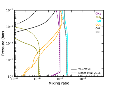
Figure 13: A comparison of the abundance profiles for the warm Jupiter 51 Eri b. The solid lines are the sulfur free model from this work and the dashed lines are the model from Moses et al. (2016). We used the temperature profile, $K_{ZZ}$ profile and UV flux profile from Moses et al. (2016). The planet has a gravity of $32\,\mathrm{ms^{-2}}$ and a solar metallicity.

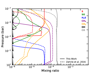
Figure 14: A comparison of the abundance profiles for the warm Jupiter 51 Eri b. The solid lines are the sulfurous model from this work and the dashed lines are the model from Zahnle et al. (2016). We used the temperature profile and UV flux profile from Moses et al. (2016), and used a constant $K_{zz}=\mathrm{10^{7}\,cm^{2}\,s^{-1}}$. The planet has a gravity of $32\,\mathrm{m\,s^{-2}}$ and a solar metallicity.

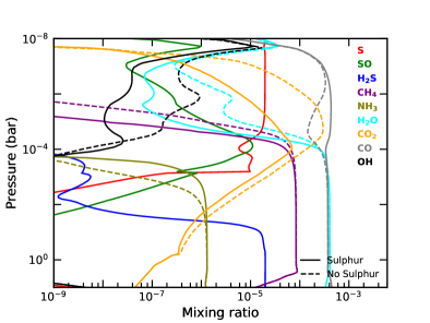
Figure 15: A comparison of the abundance profiles for a warm Jupiter model both with (solid lines) and without (dashed lines) our new sulfur network being included. This warm Jupiter uses the P-T profile and UV spectrum from Moses et al. (2016). It has a gravity of $32\,\mathrm{m\,s^{-2}}$, a solar metallicity and a constant $K_{zz}=\mathrm{10^{7}\,cm^{2}\,s^{-1}}$.

However, in Figure 15 we compare two models, with and without sulfur, both using a constant $K_{zz}=\mathrm{10^{7}\,cm^{2}\,s^{-1}}$. Our results clearly show that while the CO2 abundance in both models below $\mathrm{10^{-4}\,bar}$ are similar, above this pressure, significant differences appear. In a sulfurous atmosphere CO2 is significantly depleted, with its peak abundance five times less than in a non-sulfurous atmosphere. This is less than the difference seen between Zahnle et al. (2016) and Moses et al. (2016). Our results for CO_2 overall agree better with Moses et al. (2016), both with and without sulfur. However, the reason for the decrease in CO2 abundance with the inclusion of sulfur is the effect of the products of H_2S photo-dissociation on the abundance of OH. Both with and without sulfur, CO_2 is produced by the following reactions

$$\ce{H2O+}\ h\nu\ce{&$\, \rightarrow\, $OH+H},$$ (20)

$$\ce{CO}+\ce{OH}\ce{&$\, \rightarrow\, $}\ce{CO_{2}}+\ce{H},$$

$$\ce{H}+\ce{H}+\ce{M}\ce{&$\, \rightarrow\, $}\ce{H_{2}}+\ce{M}$$

$$\mathbf{Net:}\ \ce{H_{2}O}+\ce{CO}+h\nu\ce{&$\, \rightarrow\, $}\ce{CO_{2}}+\ce{H_{2}}.$$

The destruction is also the same regardless of the presence of sulfur, through the photo-dissociation of CO_2. What does change is the abundance of OH, which is consumed by reacting with S via

$$\ce{H_{2}S}+h\nu\ce{&$\, \rightarrow\, $}\ce{HS}+\ce{H},$$ (21)

$$\ce{HS}+\ce{H}\ce{&$\, \rightarrow\, $}\ce{H_{2}}+\ce{S},$$

$$\ce{S}+\ce{OH}\ce{&$\, \rightarrow\, $}\ce{SO}+\ce{H}.$$

The SO will diffuse upward, where it will photo-dissociate, releasing more atomic sulfur which will consume more hydroxyl radicals. It is this effect of the sulfur chemistry on the hydroxyl radicals that causes the lower abundance of CO_2 when sulfur is included. The destruction of OH via the photochemical properties of H2S explains the shift of the peak of CO_2 to higher pressures when sulfur is present.

There is one other feature of note, the H_2O spike near $\mathrm{10^{-8}\,bar}$. This occurs because our constant $K_{zz}$ places the CO homopause at $\sim 10^{-7}\,{\rm bar}$. As the CO drops off, it stops effectively self-shielding, and so CO is easily dissociated into C(^1D) and O(^1D). The O(^1D) reacts with H_2 to form H_2O. H_2O is preserved at this height, because its destruction forms OH which quickly reacts with H2 to reform H2O

$$\ce{H_{2}}+\ce{OH}\ce{&$\, \rightarrow\, $}\ce{H_{2}O}+\ce{H}.$$ (22)

This reaction dominates instead of the reaction CO + OH $\,\rightarrow\,$ CO2 + H (See Reaction 20) since the depletion of CO due to molecular diffusion means that it is no longer as efficient. This leads to H_2O peaking at $\sim 10^{-8}\,{\rm bar}$. It drops off above this height because of a combination of molecular diffusion of H_2O and photochemical destruction of OH.

6 Summary and Discussion

Our goal in this work was to construct a complete sulfur chemical network that would primarily function for the high temperatures of hot Jupiters, but that should be applicable over a large range of temperatures. By combining this network with our chemical kinetics code, Levi, described in Hobbs et al. (2019) and the H/C/O/N network STAND2019 from Rimmer & Helling (2016) and Rimmer & Rugheimer (2019) we gained the ability to find the steady-state solutions for chemical abundance in the atmospheres of a variety of hot Jupiters. We validated our new network against similar previously published models to identify the similarities and differences. We investigated the primary pathways of sulfur chemistry over a range of hot Jupiter models, and examined how the abundance of sulfur species changed with variations to the model. We also compared how the inclusion of sulfur into a hot Jupiter’s atmosphere can affect the abundance of other, non-sulfur species, potentially altering these species detectability.

We started by validating our network against previous models, including the work of Wang et al. (2017) and the work presented in Evans et al. (2018) (but made by Zahnle et al. 2016). We found our results matched nearly perfectly with Wang et al. (2017) (Figure 2), but their work only explored pressures below $\mathrm{10^{-4}\,bar}$, and so photochemistry was not considered. Similarly, we find that our results matched well with Evans et al. (2018) below $\mathrm{10^{-4}\,bar}$ (Figure 3). However, in the upper atmosphere, we find the species’ abundances follow the same general trends, but at significantly different pressures. This is inferred to be most likely due to different choices in the UV flux applied to the model.

Across a range of isothermal hot Jupiter atmospheres, we investigated the most abundant sulfur species and how this varies with the model’s parameters. In our disequilibrium atmosphere model (Figure 5) we found that from the bottom of the atmosphere until between $\mathrm{10^{-2}}$ and $\mathrm{10^{-3}\,bar}$, H2S contains nearly all of the atmosphere’s sulfur. Above this, H2S is destroyed by photochemically produced H radicals that cause atomic S to become the primary sulfur carrier for the rest of the atmosphere. Other sulfur molecules of note are S2 and HS. S2 builds up significantly around $\mathrm{10^{-3}\,bar}$, particularly on slightly cooler hot Jupiters, where for a brief pressure window it is the most abundant sulfur species. The mercapto radical, HS, is one of the few sulfur molecules whose presence may have already been detected on an exoplanet (Evans et al. 2018). We find that it builds up strongly around $\mathrm{10^{-3}\,bar}$, especially along isotherms $>1200\,\mathrm{K}$, with a maximum abundance of $\mathrm{4x10^{-3}}$ seen in our model in Figure 5.

We also examined the sensitivity of sulfur chemistry to variations in both the strength of the vertical mixing (Figure 6) and the strength of the UV flux (Figure 7) applied to the atmosphere. We found that weakening the diffusion had little effect on the sulfur species. Stronger mixing increased the abundance of H2S above $\mathrm{10^{-3}\,bar}$, while decreasing the abundance of S and S2. The effect of stronger UV irradiation is primarily to dissociate photosensitive molecules deeper into the atmosphere. Species such as H2S were up to two orders of magnitude less abundant at $\mathrm{10^{-3}\,bar}$ in more highly irradiated models.

Most sulfur species are not easily detected in exoplanet atmospheres, but that does not mean that sulfur chemistry does not matter for atmospheric retrievals. Our models have shown that the presence of sulfur in both hot and warm Jupiter atmospheres can significantly change the abundance of other, more easily detected, molecules. Of particular note are the differences we have found to the abundances of CH4, HCN and NH3 in hot Jupiters by including S in the network, as well as CO2 in warm Jupiters. We found this was due to the catalytic properties of sulfur chemistry (also seen in Zahnle et al. 2016) for CH4 and HCN, and due to the photo-shielding effect of H2S for NH3. At around a pressure of $\mathrm{10^{-3}\,bar}$ in a atmospheric model of HD 209458b (Figure 8), the abundances of NH3, CH4 and HCN in a sulfurous atmosphere dropped by several orders of magnitude when compared to their abundances in a non-sulfurous atmosphere. This is a very large change, but it occurs over a very narrow pressure window. If this intersects with the detectable range made by observations, it would be a significant and noticeable effect. But, if the detection occurred at location higher or lower in the atmosphere, no change would be noticed compared to a sulfur free case. It is also very likely that the location at which sulfur chemistry impacts these molecules is dependant upon many of the planet’s parameters: The planet’s temperature and metallicity, as well as the diffusion strength or the incoming UV flux. More testing and modelling is required to discover exactly how these parameters will alter sulfur’s effect upon these molecules.

The effect of sulfur upon CO2 in warm Jupiters is also important, first noticed when comparing the sulfurous (Zahnle et al. 2016) and non-sulfurous (Moses et al. 2016) models of 51 Eri b. We find our network predicts up to five times less CO2, due to sulfur, above $\mathrm{10^{-4}\,bar}$. Below this pressure, the loss of CO2 is present, but less significant. In this section of the upper atmosphere, we predict approximately half an order of magnitude more CO2 compared to the model in Zahnle et al. (2016). These differences in the models are again down to uncertainties in the rate constants used for our sulfur reactions.

Current observations may struggle to distinguish the effects of sulfur we predict in both hot and warm Jupiters. However, it is important that observations from the next generation of telescopes take these effects into account, since they can significantly alter the composition of the atmosphere. An understanding of the precise effects of sulfur can be difficult to reach, due to how many uncertainties there are in the reaction rate constants within the network. As we have shown, these rates can greatly affect not just other sulfur species, but other detectable species within the atmosphere. New measurements of the rate constants of these sulfur reactions need to take place to truly be able to constrain the exact effect that sulfur can have. Some of the most important reactions discussed within this work still have large divergences between their different measurements. We discuss where some of these reactions’ rate constants come from in Appendix A.

Finally, it is important to consider that while it is difficult to identify the bulk sulfur abundance without the detection of sulfur species, the effect of sulfur upon other species can be used as a method to constrain the sulfur abundance. There of course would be a large degree of degeneracy in this parameter, but it could work as a first step to limiting the sulfur abundance of exo-planets to realistic values.

Data availability

The data underlying this article is available in the article.

Appendix A Rates Discussion

Here we discuss some of the most significant sulfur chemical reaction rates in our network, their uncertainties, and where these uncertainties come from.

Photochemistry of H_2S
The photo-dissociation of H2S is one of two photochemical sulfur reactions that form the explanation for sulfur’s significant impact on other species in warm and hot Jupiters. There are a large number of works that have measured its UV cross-section, though not all of them agree what that cross-section should be. The work of Lee et al. (1987) provides an effective “backbone” to the wavelength-dependent absorption cross-sections for H_2S, and provides the lowest measured estimates for H_2S absorption of all observations, diverging from other measurements at $\lambda<172$ nm. Both Watanabe & Jursa (1964) and Wu & Chen (1998) find cross-sections below 172 nm that are a factor of 2-3 greater. Thompson et al. (1966) measures the absorption cross-section between 180 nm and 214 nm, in good agreement with other measurements at these wavelengths, though with a slight divergence between 210 – 214 nm. Wu & Chen (1998) generally agrees with most other measurements wherever one of the measurements diverges, and matches a measurement at a single (250 nm) wavelength very well (Wight & Leone, 1983). The measurements of Wu & Chen (1998) are clean and the results suggest few systematics and a very deep noise floor. For this reason the JPL database recommends using their H_2S cross-sections. More recently, Grosch et al. (2015) has made measurements at a higher resolution. These measurements diverge from Wu & Chen (1998) by a factor of 5 between 250 and 260 nm, suggesting the higher resolution has come at the cost of a higher noise floor.

Photo-chemistry of SO
The photo-dissociation of SO is the second of the important photochemical sulfur reactions. The most accurate cross-sections for SO were compiled by the Leiden database (Heays et al., 2017), based on Phillips (1981); Nee & Lee (1986); Norwood & Ng (1989). The cross-sections all agree with each other reasonably well.

H + SH -> H2 + S vs H2 + S -> H + SH
We found that the reaction H + SH -> H2 + S was significant in the pathway that lead to CO2 destruction in 51 Eri b’s atmosphere. However, in our network we choose to use this reaction’s reverse, H2 + S -> H + SH, even though it has an activation barrier. Our justification for this is that for H + SH -> H2 + S all the results are at room temperature, and all of them were measured in the 1970’s and 1980’s.

Cupitt & Glass (1970) performed a flow discharge with H_2S and O_2, and estimated the rate to be $k=1.3\times 10^{-10}\,{\rm cm^{3}\,s^{-1}}$. The experiment was subsequently revisited, and the rate constant corrected to $k=2.51\times 10^{-11}\,{\rm cm^{3}\,s^{-1}}$ in (Cupitt & Glass, 1975).

Bradley et al. (1973) also performed a flow discharge with H_2S, controlling the overall reaction with NO, attempting to isolate the individual reactions, and constrained the HS hydrogen abstraction reaction to $k=4.15\times 10^{-11}\,{\rm cm^{3}\,s^{-1}}$. Their results do not indicate any kinetic barrier or polynomial temperature dependence.

Tiee et al. (1981) used a 193 nm UV laser to dissociate H_2S, forming HS, and then subsequently measured the decay of HS. They found a maximum rate of $k<1.69\times 10^{-11}\,{\rm cm^{3}\,s^{-1}}$ .

Nicholas et al. (1979) used radio-frequency pulse discharge and found the measurement of HS decay to be $k=2.16\times 10^{-11}\,{\rm cm^{3}\,s^{-1}}$.

Langford & Oldershaw (1972) used flash photolysis and made the measurement of the HS decay to be $k=1.1\times 10^{-11}\,{\rm cm^{3}\,s^{-1}}$.

The reported rates are highly discordant, nor do they address the temperature dependence. In contrast, the reverse reaction, H2 + S -> H + SH, was constrained much better by two experiments in the late 1990’s. They were performed over a much larger temperature range, one more applicable to hot Jupiters.

Woiki & Roth (1995) used OCS/H2 pyrolysis and CS2/H2 photolysis to generate S atoms that could then react with H2. They found the reaction rate to be $k=9.96\times 10^{-10}\exp(-12070\mathrm{K}/\mathrm{T})\,{\rm cm^{3}\,s^{-1}}$ for a temperature range of $1257\,\mathrm{K}$ to $3137\,\mathrm{K}$.

Shiina et al. (1996) studied the thermal decomposition of H2S and its subsequent reactions, and found the reaction between H2 and S to be $k=2.62\times 10^{-10}\exp(-9920\mathrm{K}/\mathrm{T})\,{\rm cm^{3}\,s^{-1}}$ over a temperature range of $1050\,\mathrm{K}$ to $1660\,\mathrm{K}$.

As a result we decided that using the reaction H2 + S -> H + SH in our network was the choice offering the greatest accuracy in modelling hot Jupiters.

OH + S -> H + SO
This reaction is the last reaction important to explaining the impact of sulfur in hot and warm Jupiters. It has been mentioned in several reviews, all based on a single experimental measurement by Jourdain et al. (1979). They used a flow discharge with SO_2 and H_2O, and found $k=6.95\times 10^{-11}\,{\rm cm^{3}\,s^{-1}}$. Without a second measurement, it is difficult to determine this reaction’s uncertainties, and without uncertainties, there is no way to perform a sensitivity analysis accurately.

Appendix B The Sulfur Network

Table 3: The 3-body reactions of the sulphur network used in this work. $\alpha$, $\beta$ and $\gamma\,(\mathrm{K})$ refer to the three constants used in the arrhenius equation, such that the rate of reaction is $k=\alpha(T/300\,\mathrm{K})^{\beta}\exp(-\gamma/T)\,\mathrm{m^{3}s^{-1}}$. The reactions in this table are three body combination reactions that use a third body (M) as a catalyst. The first line of each reaction is the low pressure rate limit ($k_{0}$) and the second line is the high pressure rate limit ($k_{\infty}$) that are combined to give an overall rate via $k=\frac{k_{0}[M]}{1+\frac{k_{0}[M]}{K_{\infty}}}$. Thus $\alpha_{0}$ has units $\mathrm{m^{6}s^{-1}}$ and $\alpha_{\infty}$ has units $\mathrm{m^{3}s^{-1}}$.

No.				Reaction						$\alpha\,(m^{6}s^{-1}\,\textrm{or}\,m^{3}s^{-1})$	$\beta$	$\gamma\,(\mathrm{K})$	Reference
1	S	+	S	$\rightarrow$	S2					3.95$\times 10^{-45}$			Du et al. (2008)
	S	+	S	$\rightarrow$	S2					9.09$\times 10^{-20}$			Du et al. (2008)
2	S	+	S2	$\rightarrow$	S3					1.11$\times 10^{-42}$	-2.00		Moses et al. (2002)
	S	+	S2	$\rightarrow$	S3					3$\times 10^{-17}$			Moses et al. (2002)
3	S	+	S3	$\rightarrow$	S4					1.11$\times 10^{-42}$	-2.00		Moses et al. (2002)
	S	+	S3	$\rightarrow$	S4					3$\times 10^{-17}$			Moses et al. (2002)
4	S	+	S4	$\rightarrow$	S5					1.11$\times 10^{-42}$	-2.00		Moses et al. (2002)
	S	+	S4	$\rightarrow$	S5					3$\times 10^{-17}$			Moses et al. (2002)
5	S	+	S5	$\rightarrow$	S6					1.11$\times 10^{-42}$	-2.00		Moses et al. (2002)
	S	+	S5	$\rightarrow$	S6					3$\times 10^{-17}$			Moses et al. (2002)
6	S	+	S6	$\rightarrow$	S7					1.11$\times 10^{-42}$	-2.00		Moses et al. (2002)
	S	+	S6	$\rightarrow$	S7					3$\times 10^{-17}$			Moses et al. (2002)
7	S	+	S7	$\rightarrow$	S8					1.11$\times 10^{-42}$	-2.00		Moses et al. (2002)
	S	+	S7	$\rightarrow$	S8					3$\times 10^{-17}$			Moses et al. (2002)
8	S2	+	S2	$\rightarrow$	S4					2.2$\times 10^{-41}$			Nicholas et al. (1979)
	S2	+	S2	$\rightarrow$	S4					1$\times 10^{-16}$			Nicholas et al. (1979)
9	S2	+	S3	$\rightarrow$	S5					1.11$\times 10^{-42}$	-2.00		Moses et al. (2002)
	S2	+	S3	$\rightarrow$	S5					3$\times 10^{-17}$			Moses et al. (2002)
10	S2	+	S4	$\rightarrow$	S6					1.11$\times 10^{-42}$	-2.00		Moses et al. (2002)
	S2	+	S4	$\rightarrow$	S6					3$\times 10^{-17}$			Moses et al. (2002)
11	S2	+	S5	$\rightarrow$	S7					1.11$\times 10^{-42}$	-2.00		Moses et al. (2002)
	S2	+	S5	$\rightarrow$	S7					3$\times 10^{-17}$			Moses et al. (2002)
12	S2	+	S6	$\rightarrow$	S8					1.11$\times 10^{-42}$	-2.00		Moses et al. (2002)
	S2	+	S6	$\rightarrow$	S8					3$\times 10^{-17}$			Moses et al. (2002)
13	S3	+	S3	$\rightarrow$	S6					1$\times 10^{-42}$			Mills (1998)
	S3	+	S3	$\rightarrow$	S6					3$\times 10^{-17}$			Mills (1998)
14	S3	+	S4	$\rightarrow$	S7					1.11$\times 10^{-42}$	-2.00		Moses et al. (2002)
	S3	+	S4	$\rightarrow$	S7					3$\times 10^{-17}$			Moses et al. (2002)
15	S3	+	S5	$\rightarrow$	S8					1.11$\times 10^{-42}$	-2.00		Moses et al. (2002)
	S3	+	S5	$\rightarrow$	S8					3$\times 10^{-17}$			Moses et al. (2002)
16	S4	+	S4	$\rightarrow$	S8					1$\times 10^{-42}$			Mills (1998)
	S4	+	S4	$\rightarrow$	S8					3$\times 10^{-17}$			Mills (1998)
17	S	+	O	$\rightarrow$	SO					3.01$\times 10^{-45}$			Zhang et al. (2012)
	S	+	O	$\rightarrow$	SO					7.27$\times 10^{-20}$	-1.00		Zhang et al. (2012)
18	S	+	SO	$\rightarrow$	S2O					3.67$\times 10^{-43}$	-2.00		Moses et al. (2002)
	S	+	SO	$\rightarrow$	S2O					8.86$\times 10^{-19}$	-3.00		Moses et al. (2002)
19	S	+	H2	$\rightarrow$	H2S					1.4$\times 10^{-43}$	-1.9	2.3$\times 10^{3}$	Zahnle et al. (2016)
	S	+	H2	$\rightarrow$	H2S					1$\times 10^{-17}$			Zahnle et al. (2016)
20	SO	+	HO	$\rightarrow$	HOSO					6.45$\times 10^{-41}$	-3.48	4.90$\times 10^{2}$	Goumri et al. (1999)
	SO	+	HO	$\rightarrow$	HOSO					8.75$\times 10^{-17}$	0.50		Goumri et al. (1999)
21	SO2	+	O	$\rightarrow$	SO3					1.32$\times 10^{-41}$		1.00$\times 10^{3}$	Atkinson et al. (2004)
	SO2	+	O	$\rightarrow$	SO3					5$\times 10^{-18}$			Atkinson et al. (2004)
22	SO2	+	H	$\rightarrow$	HSO2					5.74$\times 10^{-43}$	-3.69	2.41$\times 10^{3}$	Goumri et al. (1999)
	SO2	+	H	$\rightarrow$	HSO2					2.31$\times 10^{-17}$	0.62	1.82$\times 10^{3}$	Goumri et al. (1999)
23	SO2	+	H	$\rightarrow$	HOSO					9.43$\times 10^{-40}$	-4.36	5.44$\times 10^{3}$	Goumri et al. (1999)
	SO2	+	H	$\rightarrow$	HOSO					9.13$\times 10^{-18}$	0.96	4.32$\times 10^{3}$	Goumri et al. (1999)
24	SO	+	O	$\rightarrow$	SO2					4.82$\times 10^{-43}$	-2.17		Lu et al. (2003)
	SO	+	O	$\rightarrow$	SO2					3.5$\times 10^{-17}$	0.00		Lu et al. (2003)
25	SO2	+	HO	$\rightarrow$	HSO3					3.3$\times 10^{-43}$	-4.30		Sander et al. (2006)
	SO2	+	HO	$\rightarrow$	HSO3					1.6$\times 10^{-18}$	0.00		Sander et al. (2006)
26	HS	+	NO	$\rightarrow$	HSNO					2.4$\times 10^{-43}$	-3.00		Demore et al. (1997)
	HS	+	NO	$\rightarrow$	HSNO					2.71$\times 10^{-17}$			Demore et al. (1997)
27	HS	+	O2	$\rightarrow$	HSO2					9.18$\times 10^{-46}$	-1.69		Goumri et al. (1995)
	HS	+	O2	$\rightarrow$	HSO2					2.01$\times 10^{-16}$	0.31		Goumri et al. (1995)
28	HS	+	O2	$\rightarrow$	HSOO					9.06$\times 10^{-46}$	-2.01	1.00$\times 10^{1}$	Goumri et al. (1999)
	HS	+	O2	$\rightarrow$	HSOO					3.3$\times 10^{-16}$	-0.26	1.50$\times 10^{2}$	Goumri et al. (1999)
29	HS	+	H	$\rightarrow$	H2S					1$\times 10^{-42}$	-2.00		Krasnopolsky (2007)
	HS	+	H	$\rightarrow$	H2S					2.41$\times 10^{-17}$	-3.00		Krasnopolsky (2007)
30	CS2	+	HO	$\rightarrow$	CS2OH					8$\times 10^{-43}$			Atkinson et al. (1992)
	CS2	+	HO	$\rightarrow$	CS2OH					8$\times 10^{-18}$			Atkinson et al. (1992)
31	CO	+	S	$\rightarrow$	OCS					3$\times 10^{-45}$		1.00$\times 10^{3}$	Krasnopolsky (2007)
	CO	+	S	$\rightarrow$	OCS					7.24$\times 10^{-20}$	-1.00	1.00$\times 10^{3}$	Krasnopolsky (2007)
32	CH3	+	HS	$\rightarrow$	CH3SH					6.88$\times 10^{-43}$	1.00		Shum & Benson (1985)
	CH3	+	HS	$\rightarrow$	CH3SH					1.66$\times 10^{-17}$			Shum & Benson (1985)

Table 4: The 3-body reactions of the sulphur network used in this work. $\alpha$, $\beta$ and $\gamma\,(\mathrm{K})$ refer to the three constants used in the arrhenius equation, such that the rate of reaction is $k=\alpha(T/300\,\mathrm{K})^{\beta}\exp(-\gamma/T)\,\mathrm{m^{3}s^{-1}}$. The reactions in this table are three body decomposition reactions that use a third body (M) as a catalyst and a state shift reaction. The first line of each reaction is the low pressure rate limit ($k_{0}$) and the second line is the high pressure rate limit ($k_{\infty}$) that are combined to give an overall rate via $k=\frac{k_{0}[M]}{1+\frac{k_{0}[M]}{K_{\infty}}}$. Thus $\alpha_{0}$ has units $\mathrm{m^{3}s^{-1}}$ and $\alpha_{\infty}$ has units $\mathrm{s^{-1}}$.

No.				Reaction						$\alpha\,(m^{3}s^{-1}\,\textrm{or}\,s^{-1})$	$\beta$	$\gamma\,(\mathrm{K})$	Reference
33	HSO			$\rightarrow$	H	+	SO			1.4$\times 10^{-14}$		2.95$\times 10^{4}$	Tsuchiya et al. (1994)
	HSO			$\rightarrow$	H	+	SO			3.38$\times 10^{+11}$	-1.00	2.95$\times 10^{4}$	Tsuchiya et al. (1994)
34	HOSO			$\rightarrow$	HSO2					3.18$\times 10^{-09}$	-5.64	2.79$\times 10^{4}$	Goumri et al. (1999)
	HOSO			$\rightarrow$	HSO2					3.64$\times 10^{+11}$	1.03	2.52$\times 10^{4}$	Goumri et al. (1999)
35	HSOO			$\rightarrow$	O	+	HSO			4.61$\times 10^{-10}$	-5.87	1.56$\times 10^{4}$	Goumri et al. (1999)
	HSOO			$\rightarrow$	O	+	HSO			4.53$\times 10^{+16}$	-1.07	1.43$\times 10^{4}$	Goumri et al. (1999)
36	H2S2			$\rightarrow$	HS	+	HS			3.43$\times 10^{-13}$	1.00	2.87$\times 10^{4}$	Tsuchiya et al. (1994)
	H2S2			$\rightarrow$	HS	+	HS			8.28$\times 10^{+12}$		2.87$\times 10^{4}$	Tsuchiya et al. (1994)

Table 5: The photo-chemical reactions of the sulphur network used in this work.

No.		Reaction
1	S3	$\rightarrow$	S2	+	S
2	S4	$\rightarrow$	S2	+	S2
3	SO3	$\rightarrow$	SO2	+	O
4	OCS	$\rightarrow$	S	+	CO
5	OCS	$\rightarrow$	S	+	CO
6	OCS	$\rightarrow$	S	+	CO
7	OCS	$\rightarrow$	CS	+	O
8	OCS	$\rightarrow$	CS	+	O(^1D)
9	S2	$\rightarrow$	S	+	S
10	S2O	$\rightarrow$	SO	+	S
11	S2O	$\rightarrow$	S2	+	O
12	SO	$\rightarrow$	S	+	O
13	CS2	$\rightarrow$	CS	+	S
14	SO2	$\rightarrow$	SO	+	O
15	SO2	$\rightarrow$	S	+	O2
16	H2S	$\rightarrow$	HS	+	H
17	CH3SH	$\rightarrow$	CH3	+	HS

Table 6: The 2-body reactions of the sulphur network used in this work. $\alpha\,(\mathrm{m^{3}s^{-1}})$, $\beta$ and $\gamma\,(\mathrm{K})$ refer to the three constants used in the arrhenius equation, such that the rate of reaction is $k=\alpha(T/300\,\mathrm{K})^{\beta}\exp(-\gamma/T)\,\mathrm{m^{3}s^{-1}}$. For the reactions with multiple sources, we have blended data from both sources to extend the applicable temperature range for the reaction.

No.				Reaction						$\alpha\,(m^{3}s^{-1})$	$\beta$	$\gamma\,(\mathrm{K})$	Reference
1	S	+	S3	$\rightarrow$	S2	+	S2			8$\times 10^{-17}$			Moses et al. (2002)
2	S	+	S4	$\rightarrow$	S2	+	S3			8$\times 10^{-17}$			Moses et al. (2002)
3	S	+	S5	$\rightarrow$	S2	+	S4			5$\times 10^{-17}$		2.00$\times 10^{2}$	Moses et al. (2002)
4	S	+	S6	$\rightarrow$	S2	+	S5			5$\times 10^{-17}$		3.00$\times 10^{2}$	Moses et al. (2002)
5	S	+	S7	$\rightarrow$	S2	+	S6			4$\times 10^{-17}$		2.00$\times 10^{2}$	Moses et al. (2002)
6	S	+	S8	$\rightarrow$	S2	+	S7			4$\times 10^{-17}$		4.00$\times 10^{2}$	Moses et al. (2002)
7	S	+	S5	$\rightarrow$	S3	+	S3			3$\times 10^{-17}$		2.00$\times 10^{2}$	Moses et al. (2002)
8	S	+	S6	$\rightarrow$	S3	+	S4			3$\times 10^{-17}$		3.00$\times 10^{2}$	Moses et al. (2002)
9	S	+	S7	$\rightarrow$	S3	+	S5			2$\times 10^{-17}$		2.00$\times 10^{2}$	Moses et al. (2002)
10	S	+	S8	$\rightarrow$	S3	+	S6			2$\times 10^{-17}$		4.00$\times 10^{2}$	Moses et al. (2002)
11	S	+	S7	$\rightarrow$	S4	+	S4			2$\times 10^{-17}$		2.00$\times 10^{2}$	Moses et al. (2002)
12	S	+	S8	$\rightarrow$	S4	+	S5			2$\times 10^{-17}$		4.00$\times 10^{2}$	Moses et al. (2002)
13	S2	+	S8	$\rightarrow$	S5	+	S5			1$\times 10^{-17}$		1.40$\times 10^{3}$	Moses et al. (2002)
14	S3	+	S5	$\rightarrow$	S2	+	S6			4$\times 10^{-17}$		2.00$\times 10^{2}$	Moses et al. (2002)
15	S3	+	S7	$\rightarrow$	S2	+	S8			3$\times 10^{-17}$		2.00$\times 10^{2}$	Moses et al. (2002)
16	S3	+	S7	$\rightarrow$	S4	+	S6			1$\times 10^{-17}$		2.00$\times 10^{2}$	Moses et al. (2002)
17	S3	+	S4	$\rightarrow$	S2	+	S5			4$\times 10^{-17}$		2.00$\times 10^{2}$	Moses et al. (2002)
18	S3	+	S6	$\rightarrow$	S2	+	S7			4$\times 10^{-18}$		3.00$\times 10^{2}$	Moses et al. (2002)
19	S3	+	S7	$\rightarrow$	S5	+	S5			1$\times 10^{-17}$		2.00$\times 10^{2}$	Moses et al. (2002)
20	S4	+	S5	$\rightarrow$	S2	+	S7			2$\times 10^{-18}$		2.00$\times 10^{2}$	Moses et al. (2002)
21	S4	+	S6	$\rightarrow$	S2	+	S8			2$\times 10^{-18}$		3.00$\times 10^{2}$	Moses et al. (2002)
22	S4	+	S5	$\rightarrow$	S3	+	S6			2$\times 10^{-18}$		2.00$\times 10^{2}$	Moses et al. (2002)
23	S4	+	S7	$\rightarrow$	S3	+	S8			5$\times 10^{-18}$		2.00$\times 10^{2}$	Moses et al. (2002)
24	S4	+	S6	$\rightarrow$	S5	+	S5			2$\times 10^{-18}$		3.00$\times 10^{2}$	Moses et al. (2002)
25	S4	+	S7	$\rightarrow$	S5	+	S6			5$\times 10^{-18}$		2.00$\times 10^{2}$	Moses et al. (2002)
26	O	+	S2	$\rightarrow$	S	+	SO			2$\times 10^{-17}$		8.40$\times 10^{1}$	Craven & Murrell (1987)
27	O	+	S3	$\rightarrow$	S2	+	SO			8$\times 10^{-17}$			Moses et al. (2002)
28	O	+	S4	$\rightarrow$	S3	+	SO			8$\times 10^{-17}$			Moses et al. (2002)
29	O	+	S5	$\rightarrow$	S4	+	SO			8$\times 10^{-17}$		2.00$\times 10^{2}$	Moses et al. (2002)
30	O	+	S6	$\rightarrow$	S5	+	SO			8$\times 10^{-17}$		3.00$\times 10^{2}$	Moses et al. (2002)
31	O	+	S7	$\rightarrow$	S6	+	SO			8$\times 10^{-17}$		2.00$\times 10^{2}$	Moses et al. (2002)
32	O	+	S8	$\rightarrow$	S7	+	SO			8$\times 10^{-17}$		4.00$\times 10^{2}$	Moses et al. (2002)
33	S	+	O2	$\rightarrow$	SO	+	O			2.51$\times 10^{-17}$		1.84$\times 10^{3}$	Miyoshi et al. (1996)
34	S	+	SO2	$\rightarrow$	SO	+	SO			9.77$\times 10^{-18}$		4.54$\times 10^{3}$	Isshiki et al. (2003)
35	S	+	H2	$\rightarrow$	H	+	HS			3.04$\times 10^{-19}$	2.70	6.46$\times 10^{3}$	Shiina et al. (1996) and Woiki & Roth (1995)
36	S	+	OCS	$\rightarrow$	CO	+	S2			1.35$\times 10^{-19}$	2.70	1.20$\times 10^{3}$	Shiina et al. (1996) and Lu et al. (2006)
37	S	+	CS2	$\rightarrow$	CS	+	S2			2.82$\times 10^{-16}$		5.92$\times 10^{3}$	Woiki & Roth (1995)
38	S	+	C2H6	$\rightarrow$	HS	+	C2H5			2.04$\times 10^{-16}$		7.42$\times 10^{3}$	Tsuchiya et al. (1996)
39	S	+	CH4	$\rightarrow$	HS	+	CH3			3.39$\times 10^{-16}$		1.00$\times 10^{4}$	Tsuchiya et al. (1996)
40	S	+	HS	$\rightarrow$	S2	+	H			4.98$\times 10^{-18}$			Nicholas et al. (1979)
41	S	+	HO2	$\rightarrow$	SO	+	HO			5.84$\times 10^{-17}$			Zhang et al. (2012)
42	S	+	SO3	$\rightarrow$	SO2	+	SO			1$\times 10^{-22}$			Moses et al. (2002)
43	S	+	HO	$\rightarrow$	SO	+	H			6.6$\times 10^{-17}$			Demore et al. (1997)
44	S	+	S2O	$\rightarrow$	S2	+	SO			1$\times 10^{-18}$		1.20$\times 10^{3}$	Moses et al. (2002)
45	S	+	O3	$\rightarrow$	SO	+	O2			1.2$\times 10^{-17}$			Atkinson et al. (2004)
46	S3	+	CO	$\rightarrow$	OCS	+	S2			1$\times 10^{-17}$		2.00$\times 10^{4}$	Krasnopolsky (2007)
47	S3	+	H	$\rightarrow$	HS	+	S2			1.2$\times 10^{-16}$		1.95$\times 10^{3}$	Krasnopolsky (2007)
48	HS	+	HS	$\rightarrow$	H2S	+	S			1.5$\times 10^{-17}$			Schofield (1973)
49	HS	+	HO	$\rightarrow$	H2O	+	S			2.5$\times 10^{-18}$			Krasnopolsky (2007)
50	HS	+	O	$\rightarrow$	H	+	SO			1.3$\times 10^{-16}$			Tsuchiya et al. (1994)
51	HS	+	NO2	$\rightarrow$	NO	+	HSO			6.49$\times 10^{-17}$			Atkinson et al. (2004)
52	HS	+	N2O	$\rightarrow$	N2	+	HSO			5$\times 10^{-22}$			Herndon et al. (1999)
53	HS	+	O3	$\rightarrow$	O2	+	HSO			1.1$\times 10^{-17}$		2.80$\times 10^{2}$	Wang & Howard (1990)
54	HS	+	O2	$\rightarrow$	O	+	HSO			3.11$\times 10^{-17}$		9.02$\times 10^{3}$	Tsuchiya et al. (1997)
55	HS	+	O2	$\rightarrow$	HO	+	SO			4$\times 10^{-25}$			Demore et al. (1997)
56	HS	+	CO	$\rightarrow$	OCS	+	H			4.15$\times 10^{-20}$		7.66$\times 10^{3}$	Kurbanov & Mamedov (1995)
57	HS	+	H2CS	$\rightarrow$	H2S	+	HCS			8.14$\times 10^{-17}$		3.18$\times 10^{3}$	Vandeputte et al. (2010)

Table 7: The 2-body reactions of the sulphur network used in this work. $\alpha\,(\mathrm{m^{3}s^{-1}})$, $\beta$ and $\gamma\,(\mathrm{K})$ refer to the three constants used in the arrhenius equation, such that the rate of reaction is $k=\alpha(T/300\,\mathrm{K})^{\beta}\exp(-\gamma/T)\,\mathrm{m^{3}s^{-1}}$.

No.				Reaction						$\alpha\,(m^{3}s^{-1})$	$\beta$	$\gamma\,(\mathrm{K})$	Reference
58	H2S	+	O	$\rightarrow$	H	+	HSO			5$\times 10^{-16}$		3.85$\times 10^{3}$	Tsuchiya et al. (1994)
59	H2S	+	O	$\rightarrow$	HO	+	HS			2.01$\times 10^{-16}$		3.85$\times 10^{3}$	Tsuchiya et al. (1994)
60	H2S	+	H	$\rightarrow$	H2	+	HS			3.07$\times 10^{-18}$	2.10	3.52$\times 10^{2}$	Yoshimura et al. (1992)
61	H2S	+	O2	$\rightarrow$	HO2	+	HS			3.1$\times 10^{-18}$	2.76	1.92$\times 10^{4}$	Montoya et al. (2005)
62	H2S	+	HO	$\rightarrow$	H2O	+	HS			1.61$\times 10^{-17}$		5.40$\times 10^{2}$	Mousavipour et al. (2003)
63	H2S	+	HO2	$\rightarrow$	H2O	+	HSO			5$\times 10^{-18}$			Bulatov et al. (1990)
64	H2S	+	CH3	$\rightarrow$	CH4	+	HS			1.05$\times 10^{-19}$	1.20	7.22$\times 10^{2}$	Mousavipour et al. (2003)
65	H2S	+	SO2	$\rightarrow$	H2O	+	S2O			1.09$\times 10^{-19}$	1.86	1.90$\times 10^{4}$	Sendt & Haynes (2005)
66	H2S	+	S2O	$\rightarrow$	H2O	+	S3			7.08$\times 10^{-19}$	1.51	1.71$\times 10^{4}$	Sendt & Haynes (2005)
67	SO	+	HO2	$\rightarrow$	SO2	+	HO			2.8$\times 10^{-17}$			Zhang et al. (2012)
68	SO	+	S3	$\rightarrow$	S2O	+	S2			1$\times 10^{-18}$			Moses et al. (2002)
69	SO	+	O3	$\rightarrow$	SO2	+	O2			4.5$\times 10^{-18}$		1.17$\times 10^{3}$	Atkinson et al. (2004)
70	SO	+	O3	$\rightarrow$	SO2	+	O2(a^1Δg)			3.6$\times 10^{-19}$		1.10$\times 10^{3}$	Sander et al. (2006)
71	SO	+	O2	$\rightarrow$	SO2	+	O			4.37$\times 10^{-20}$	1.40	1.87$\times 10^{3}$	Garland (1998)
72	SO	+	CO2	$\rightarrow$	SO2	+	CO			1.5$\times 10^{-17}$		2.20$\times 10^{4}$	Bauer et al. (1971)
73	SO	+	NO2	$\rightarrow$	SO2	+	NO			1.4$\times 10^{-17}$			Atkinson et al. (2004)
74	SO	+	SO3	$\rightarrow$	SO2	+	SO2			2$\times 10^{-21}$			Chung et al. (1975)
75	SO2	+	H	$\rightarrow$	HO	+	SO			4.58$\times 10^{-14}$	-2.30	1.56$\times 10^{4}$	Blitz et al. (2006)
76	SO2	+	NO3	$\rightarrow$	SO3	+	NO2			1.8$\times 10^{-28}$			Kurten et al. (2010)
77	SO2	+	O3	$\rightarrow$	SO3	+	O2			3.01$\times 10^{-18}$		7.00$\times 10^{3}$	Demore et al. (1997)
78	SO2	+	HO2	$\rightarrow$	HO	+	SO3			2.26$\times 10^{-19}$		3.42$\times 10^{3}$	Hwang et al. (2010)
79	SO2	+	HO2	$\rightarrow$	O2	+	HOSO			8.6$\times 10^{-16}$		5.23$\times 10^{3}$	Wang & Hou (2005)
80	SO2	+	O3	$\rightarrow$	SO3	+	O2(a^1Δg)			6$\times 10^{-20}$		7.00$\times 10^{3}$	Zhang et al. (2012)
81	SO2	+	O(^1D)	$\rightarrow$	SO	+	O2			1.3$\times 10^{-16}$			Moses et al. (2002)
82	SO2	+	NO2	$\rightarrow$	SO3	+	NO			2$\times 10^{-32}$			Penzhorn & Canosa (1983)
83	SO3	+	O	$\rightarrow$	SO2	+	O2			1.06$\times 10^{-19}$	2.57	1.47$\times 10^{4}$	Hindiyarti et al. (2007)
84	SO3	+	H	$\rightarrow$	HO	+	SO2			1.46$\times 10^{-17}$	1.22	1.67$\times 10^{3}$	Hindiyarti et al. (2007)
85	SO3	+	S2	$\rightarrow$	S2O	+	SO2			2$\times 10^{-22}$			Moses et al. (2002)
86	SO3	+	CO	$\rightarrow$	CO2	+	SO2			1$\times 10^{-17}$		1.30$\times 10^{4}$	Krasnopolsky VA (1994)
87	S2O	+	O	$\rightarrow$	SO	+	SO			1.7$\times 10^{-18}$			Mills (1998)
88	S2O	+	S2O	$\rightarrow$	S3	+	SO2			1$\times 10^{-20}$			Mills (1998)
89	OCS	+	O	$\rightarrow$	CO	+	SO			1.99$\times 10^{-17}$		2.15$\times 10^{3}$	Wei & Timmons (1975)
90	OCS	+	O	$\rightarrow$	CO2	+	S			8.3$\times 10^{-17}$		5.53$\times 10^{3}$	Singleton & Cvetanovic (1988)
91	OCS	+	C	$\rightarrow$	CO	+	CS			1.01$\times 10^{-16}$			Dorthe et al. (1991)
92	OCS	+	NO3	$\rightarrow$	CO	+	SO	+	NO2	1$\times 10^{-22}$			Atkinson et al. (2004)
93	OCS	+	HO	$\rightarrow$	CO2	+	HS			1.1$\times 10^{-19}$		1.20$\times 10^{3}$	Sander et al. (2006)
94	CS	+	O	$\rightarrow$	CO	+	S			2.61$\times 10^{-16}$		7.58$\times 10^{2}$	Lilenfeld & Richardson (1977)
95	CS	+	HO	$\rightarrow$	H	+	OCS			1.7$\times 10^{-16}$			Wakelam et al. (2015)
96	CS	+	HO	$\rightarrow$	CO	+	HS			3$\times 10^{-17}$			Wakelam et al. (2015)
97	CS	+	C	$\rightarrow$	S	+	C2			1.44$\times 10^{-17}$	0.5	2.04$\times 10^{4}$	Wakelam et al. (2015)
98	CS	+	C2H3	$\rightarrow$	H2C3S	+	H			1.7$\times 10^{-18}$		4.00$\times 10^{2}$	Wakelam et al. (2015)
99	CS	+	CH	$\rightarrow$	S	+	C2H			5$\times 10^{-17}$			Wakelam et al. (2015)
100	CS	+	HN	$\rightarrow$	S	+	HNC			1$\times 10^{-17}$		1.20$\times 10^{3}$	Wakelam et al. (2015)
101	CS	+	NO2	$\rightarrow$	OCS	+	NO			7.61$\times 10^{-23}$			Black et al. (1983)
102	CS	+	O3	$\rightarrow$	OCS	+	O2			3.01$\times 10^{-22}$			Black et al. (1983)
103	CS	+	O2	$\rightarrow$	OCS	+	O			2.62$\times 10^{-22}$		1.86$\times 10^{3}$	Richardson (1975)
104	CS2	+	O	$\rightarrow$	CS	+	SO			2.76$\times 10^{-17}$		6.44$\times 10^{2}$	Wei & Timmons (1975)
105	CS2	+	O	$\rightarrow$	CO	+	S2			1.08$\times 10^{-19}$			Cooper & Hershberger (1992)
106	CS2	+	O	$\rightarrow$	OCS	+	S			3.65$\times 10^{-18}$		5.83$\times 10^{3}$	Singleton & Cvetanovic (1988)
107	CS2	+	HO	$\rightarrow$	OCS	+	HS			1.7$\times 10^{-21}$			Atkinson et al. (2004)
108	HSO3	+	O2	$\rightarrow$	HO2	+	SO3			1.3$\times 10^{-18}$		3.30$\times 10^{2}$	Atkinson et al. (1992)
109	HSO	+	NO2	$\rightarrow$	NO	+	HSO2			9.6$\times 10^{-18}$			Demore et al. (1997)
110	HSO	+	O3	$\rightarrow$	O2	+	O2	+	HS	2.54$\times 10^{-19}$		3.84$\times 10^{2}$	Wang & Howard (1990)
111	HSO2	+	O2	$\rightarrow$	HO2	+	SO2			3.01$\times 10^{-19}$			Demore et al. (1997)
112	HSOO	+	O2	$\rightarrow$	HO2	+	SO2			3.01$\times 10^{-19}$			Demore et al. (1997)
113	H2CS	+	H	$\rightarrow$	H2	+	HCS			9.33$\times 10^{-17}$		3.57$\times 10^{3}$	Vandeputte et al. (2010)
114	H2CS	+	CH3	$\rightarrow$	CH4	+	HCS			2.57$\times 10^{-17}$		4.93$\times 10^{3}$	Vandeputte et al. (2010)
115	CH3SH	+	H	$\rightarrow$	CH3	+	H2S			1.15$\times 10^{-17}$		8.41$\times 10^{2}$	Amano et al. (1983)

References

- Agúndez et al. (2014) Agúndez M., Parmentier V., Venot O., Hersant F., Selsis F., 2014, A&A, 564, A73
- Amano et al. (1983) Amano A., Yamada M., Hashimoto K., Sugiura K., 1983, NIPPON KAGAKU KAISHI, 1983, 385
- Asplund et al. (2009) Asplund M., Grevesse N., Sauval A. J., Scott P., 2009, ARA&A, 47, 481
- Atkinson et al. (1992) Atkinson R., Baulch D. L., Cox R. A., Hampson R. F., Kerr J. A., Troe J., 1992, Journal of Physical and Chemical Reference Data, 21, 1125
- Atkinson et al. (2004) Atkinson R., et al., 2004, Atmospheric Chemistry and Physics, 4, 1461
- Bauer et al. (1971) Bauer S., Jeffers P., Lifshitz A., Yadava B., 1971, Symposium (International) on Combustion, 13, 417
- Black et al. (1983) Black G., Jusinski L., Slanger T., 1983, Chemical Physics Letters, 102, 64
- Blitz et al. (2006) Blitz M. A., Hughes K. J., Pilling M. J., Robertson S. H., 2006, The Journal of Physical Chemistry A, 110, 2996
- Bradley et al. (1973) Bradley J. N., Trueman S. P., Whytock D. A., Zaleski T. A., 1973, Journal of the Chemical Society, Faraday Transactions 1: Physical Chemistry in Condensed Phases, 69, 416
- Bulatov et al. (1990) Bulatov V., Vereshchuk S., Dzegilenko F., Sarkisov O., Khabarov V., 1990, KHIMICHESKAYA FIZIKA, 9, 1214
- Cabot et al. (2019) Cabot S. H. C., Madhusudhan N., Hawker G. A., Gandhi S., 2019, MNRAS, 482, 4422
- Chase (1998) Chase M., 1998, NIST-JANAF Thermochemical Table. American Institute of Physics
- Chung et al. (1975) Chung K., Calvert J. G., Bottenheim J. W., 1975, International Journal of Chemical Kinetics, 7, 161
- Cooper & Hershberger (1992) Cooper W. F., Hershberger J. F., 1992, The Journal of Physical Chemistry, 96, 5405
- Craven & Murrell (1987) Craven W., Murrell J. N., 1987, J. Chem. Soc., Faraday Trans. 2, 83, 1733
- Cupitt & Glass (1970) Cupitt L., Glass G., 1970, Transactions of the Faraday Society, 66, 3007
- Cupitt & Glass (1975) Cupitt L., Glass G., 1975, Int. J. Chem. Kinet.;(United States), 7
- Demore et al. (1997) Demore W., et al., 1997, JPL Publication, 90
- Dorthe et al. (1991) Dorthe G., Caubet P., Vias T., Barrere B., Marchais J., 1991, The Journal of Physical Chemistry, 95, 5109
- Drummond et al. (2018) Drummond B., Mayne N. J., Manners J., Baraffe I., Goyal J., Tremblin P., Sing D. K., Kohary K., 2018, ApJ, 869, 28
- Du et al. (2008) Du S., Francisco J. S., Shepler B. C., Peterson K. A., 2008, The Journal of chemical physics, 128, 204306
- Evans et al. (2018) Evans T. M., et al., 2018, AJ, 156, 283
- Gao et al. (2017) Gao P., Marley M. S., Zahnle K., Robinson T. D., Lewis N. K., 2017, AJ, 153, 139
- Garland (1998) Garland N. L., 1998, Chemical Physics Letters, 290, 385
- Goumri et al. (1995) Goumri A., Rocha J.-D. R., Marshall P., 1995, The Journal of Physical Chemistry, 99, 10834
- Goumri et al. (1999) Goumri A., Rocha J.-D. R., Laakso D., Smith C. E., Marshall P., 1999, The Journal of Physical Chemistry A, 103, 11328
- Grosch et al. (2015) Grosch H., Fateev A., Clausen S., 2015, J. Quant. Spectrosc. Radiative Transfer, 154, 28
- Guilluy et al. (2019) Guilluy G., Sozzetti A., Brogi M., Bonomo A. S., Giacobbe P., Claudi R., Benatti S., 2019, A&A, 625, A107
- Hawker et al. (2018) Hawker G. A., Madhusudhan N., Cabot S. H. C., Gandhi S., 2018, ApJ, 863, L11
- He et al. (2020) He C., et al., 2020, in AAS/Division for Planetary Sciences Meeting Abstracts. p. 403.04
- Heays et al. (2017) Heays A. N., Bosman A. D., van Dishoeck E. F., 2017, A&A, 602, A105
- Herndon et al. (1999) Herndon S. C., Froyd K. D., Lovejoy E. R., Ravishankara A. R., 1999, The Journal of Physical Chemistry A, 103, 6778
- Hindiyarti et al. (2007) Hindiyarti L., Glarborg P., Marshall P., 2007, The Journal of Physical Chemistry A, 111, 3984
- Hobbs et al. (2019) Hobbs R., Shorttle O., Madhusudhan N., Rimmer P., 2019, MNRAS, 487, 2242
- Hodgskiss et al. (2019) Hodgskiss M. S. W., Crockford P. W., Peng Y., Wing B. A., Horner T. J., 2019, Proceedings of the National Academy of Science, 116, 17207
- Hu et al. (2012) Hu R., Seager S., Bains W., 2012, ApJ, 761, 166
- Hu et al. (2013) Hu R., Seager S., Bains W., 2013, ApJ, 769, 6
- Hwang et al. (2010) Hwang S. M., Cooke J. A., De Witt K. J., Rabinowitz M. J., 2010, International Journal of Chemical Kinetics, 42, 168
- Irwin (1999) Irwin P. G. J., 1999, Surveys in Geophysics, 20, 505
- Isshiki et al. (2003) Isshiki N., Murakami Y., Tsuchiya K., Tezaki A., Matsui H., 2003, The Journal of Physical Chemistry A, 107, 2464
- Jourdain et al. (1979) Jourdain J., Bras G. L., Combourieu J., 1979, International Journal of Chemical Kinetics, 11, 569
- Krasnopolsky (2007) Krasnopolsky V. A., 2007, Icarus, 191, 25
- Krasnopolsky VA (1994) Krasnopolsky VA P. J., 1994, Icarus
- Kurbanov & Mamedov (1995) Kurbanov M., Mamedov K., 1995, Kinetics and Catalysis - KINET CATAL-ENGL TR, 36, 455
- Kurten et al. (2010) Kurten T., Lane J. R., Jorgensen S., Kjaergaard H. G., 2010, Phys. Chem. Chem. Phys., 12, 12833