Floquet chiral hinge modes and their interplay with Weyl physics in a three-dimensional lattice

Abstract

We demonstrate that a three dimensional time-periodically driven (Floquet) lattice can exhibit chiral hinge states and describe their interplay with Weyl physics. A peculiar type of the hinge states are enforced by the repeated boundary reflections with lateral Goos-Hänchen like shifts occurring at the second-order boundaries of our system. Such chiral hinge modes coexist in a wide range of parameters regimes with Fermi arc surface states connecting a pair of Weyl points in a two-band model. We find numerically that these modes still preserve their locality along the hinge and their chiral nature in the presence of local defects and other parameter changes. We trace the robustness of such chiral hinge modes to special band structure unique in a Floquet system allowing all the eigenstates to be localized in quasi-one-dimensional regions parallel to each other when open hinge boundaries are introduced. The implementation of a model featuring both the second-order Floquet skin effect and the Weyl physics is straightforward with ultracold atoms in optical superlattices.

I Introduction

In recent years, researches have demonstrated that time-periodically driven (Floquet) systems can show intriguing and unique effects that find no counterparts in non-driven systems. Examples include anomalous Floquet topological insulators featuring robust chiral edge modes for vanishing Chern numbers Kitagawa et al. (2010); Rudner et al. (2013); Roy and Harper (2017a); Yao et al. (2017a); Mukherjee et al. (2017a); Peng et al. (2016); Maczewsky et al. (2016); von Keyserlingk and Sondhi (2016); Else and Nayak (2016); Potirniche et al. (2017); Wintersperger et al. (2020) and discrete time crystals Sacha (2015); Khemani et al. (2016); Else et al. (2016); Yao et al. (2017b); Zhang et al. (2017); Choi et al. (2017); Rovny et al. (2018); Ho et al. (2017); Huang et al. (2018); Sacha and Zakrzewski (2017); Yao and Nayak (2018); Sacha (2020). The periodic driving shifts the fundamental theoretical framework from focusing on Hamiltonian eigenproblems to the unitary evolution operators genuinely depending on time, resulting in a plethora of new concepts and methods such as space-time winding numbers Rudner et al. (2013) and spectral pairing von Keyserlingk et al. (2016). In this context, it appears natural and tantalizing to explore possible new classes of periodically driven systems that go beyond descriptions by traditional theories.

In this paper, we show that time-periodic driving of a three dimensional (3D) lattice can give rise to a new type of chiral hinge (i.e. second-order boundary) states. Such hinge modes are associated with a reorganization of the Floquet eigenstates in response to shifting from periodic to open boundary conditions. The phenomena may be intuitive understood starting from a fine-tuned point, where the quasi-energy bands have linear dispersion along only one direction and remain flat along the other two. When open hinge boundaries are introduced, this leads to reorganization of eigenstates of the system into a set states of the quasi-one-dimensional nature orienting parallel to each other and located at various distances from the hinge. Among them, the modes closest to certain lattice hinge correspond to trajectories with uni-directional (chiral) motion within each driving period. Importantly, the counterpart of such a chiral hinge mode with opposite chirality resides on the other side of the lattice. Therefore the chiral transport carried by these hinge modes would be preserved under a small perturbation assuming it does not mix eigenstates spatially separating far away from each other. Such a robustness is verified numerically by observing the particle transport encountering perturbations in the form of parameter change and local defects.

Surface modes exist widely under various circumstances, and it is helpful to mention what may be different in our system. First, unlike the case of (Floquet) higher-order topological phases Benalcazar et al. (2017a, b); Khalaf (2018); Yan et al. (2018); Wang et al. (2018); Huang and Liu (2020); Peng and Refael (2018); Bomantara et al. (2019); Rodriguez-Vega et al. (2019); Plekhanov et al. (2019), the hinge states studied here are formed inside the bulk spectrum near zero quasi-energy, as can be seen in Fig. 2 column (2). Their existence and robustness, therefore, requires a new theoretical explanation without invoking a bulk gap. Secondly, the localization of modes at the boundaries resembles the non-Hermitian skin effect Yao and Wang (2018); Bergholtz et al. (2020); Ashida et al. (2020); Kawabata et al. (2020); Wu et al. (2019); Xiao et al. (2020); Song et al. (2019), with a notable difference being the reduced dimensionality which may be thought of as a higher-order skin effect. Thirdly, different from one-dimensional (1D) periodically driven lattices Budich et al. (2017) exhibiting helical modes, in our system the modes with opposite chirality residing at opposite hinges are well spatially separated, so the scattering due to a local perturbation would not reverse the chiral direction of the particle transport.

The aforementioned hinge states coexist with Weyl physics Armitage et al. (2018); Anderson et al. (2012, 2013); Dubček et al. (2015); Sun et al. (2018); Higashikawa et al. (2019); Lu et al. (2020); Wang et al. ; Zhu et al. ; Lang et al. (2017) when parameters are tuned away from the limit of uni-directional dispersionless motion. In that case a pair of Weyl points is created at quasienergy $\pi$ leading to a Fermi-arc surface (i.e. first-order boundary) states. We find numerically that the parameter regime of the hinge states overlaps considerably with that for the Weyl physics, signaling a simultaneous observation of both phenomena in a unified experimental setting.

The model system proposed and studied here consists of a simple, stepwise modulation of tunneling matrix elements involving six steps. It generalizes to three dimensions a two-dimensional lattice model introduced by Rudner et. al. Rudner et al. (2013) for studying anomalous Floquet topolgical insulators (see also Ref. Kitagawa et al. (2010)). The latter 2D tunnel modulation has been recently applied to ultracold atoms for the realization of anomalous topological band structures Wintersperger et al. (2020). Our 3D model can equally be implemented with ultracold atoms using such a stepwise tunnel modulation, now in 3D optical superlattices. Furthermore, besides giving rise to a new phenomenon, the unconventional chiral second-order Floquet skin effect, the model proposed here also provides a simple recipe for the implementation of Weyl physics by means of time-periodic driving.

This paper is structured as follows. In the next Section II a 3D periodically driven lattice is defined. Subsequently the characteristic features of the bulk and hinge physics are considered in Secs. III and IV. The experimental implementation of our model, using ultracold atoms in modulated superlattices, is discussed in Sec. V, followed by the Concluding Section VI. Additional technical details are presented in four Appendices A – D.

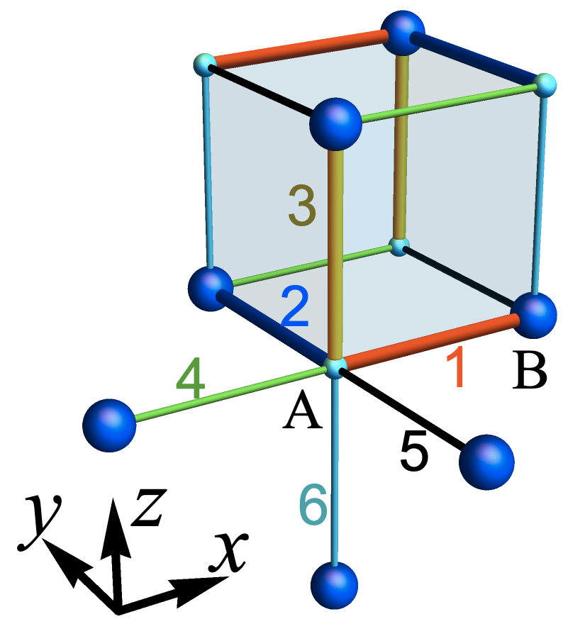
(a) Driving

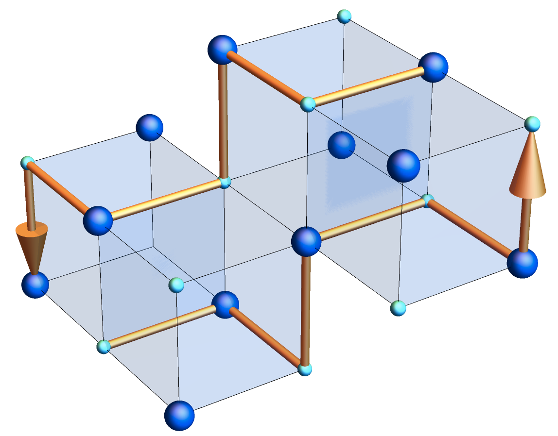
(b) Bulk dynamics

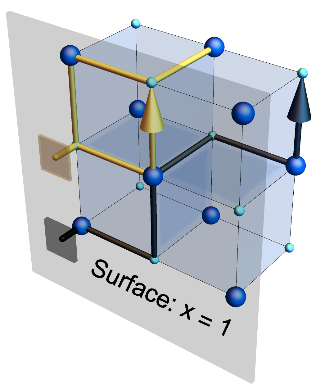
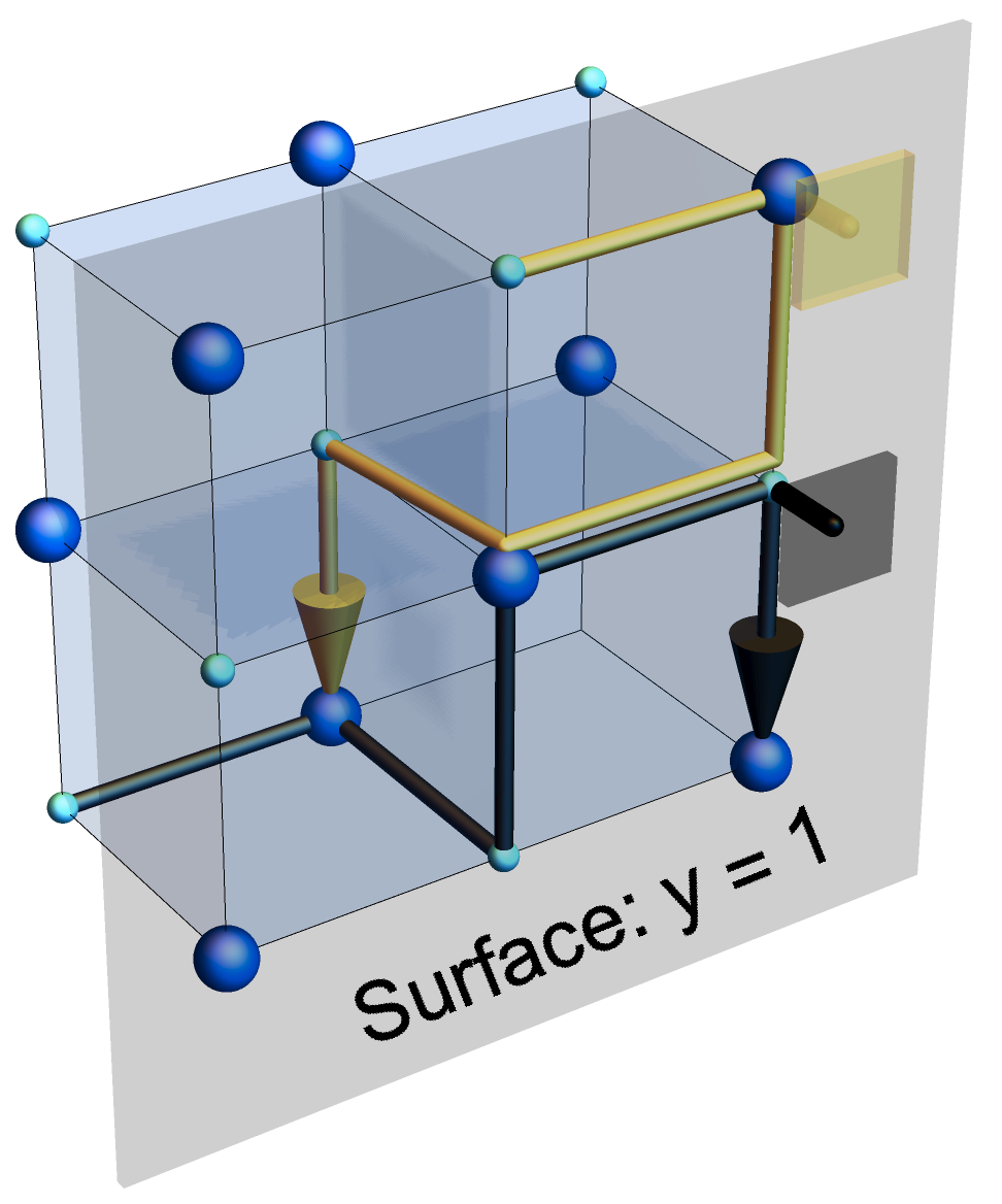
(c) Reflection by open boundary surfaces at $x=1$ and $y=1$ accompanied by sublattice changes $B\rightarrow A$ and $A\rightarrow B$, respectively.

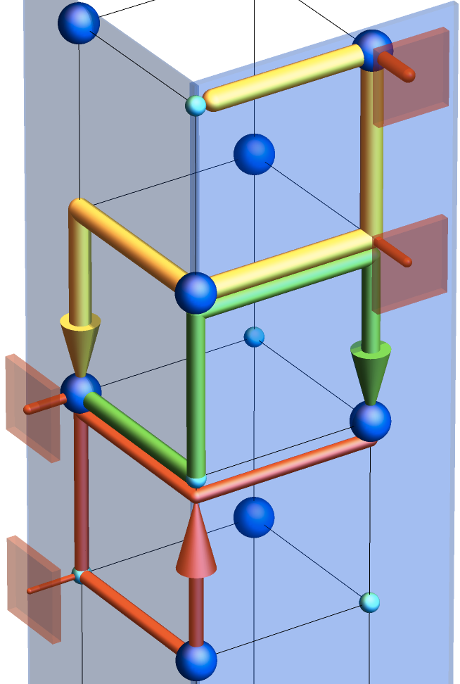
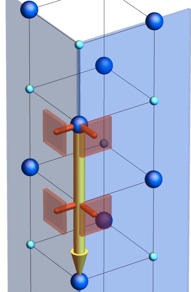
(d) Hinge dynamics

Figure 1: (a) Bonds connected during the driving steps 1 to 6. (b) Bulk trajectories within a Floquet cycle at the fine tuned point $\phi=\pi/2$. Depending on the starting sublattice, particles will travel in opposite directions along the cubic diagonal $\mathbf{d}=(1,-1,1)$ within a period. (c) Trajectories at the same $\phi=\pi/2$ but with a surface termination (open boundary). Particles starting from sublattice $A$ (or $B$) near the $y=1$ (or $x=1$) surface would have their dynamics impeded by the open boundary at a certain driving step. That results in a switch of sublattice after a Floquet cycle, and therefore the direction of the trajectory is reversed after the reflection from the surface. (d) The hinge formed by two intersecting terminating surfaces renders uni-directional modes at $\phi=\pi/2$. The figure shows two of the modes closest to the hinge starting at a site of $B$ (lower plot) or $A$ (upper plot) sublattices directly at the hinge. Each color for the arrow denotes one Floquet cycle. The lower-panel of (d) shows the mode situated directly at the hinge which undergoes a uni-directional motion along $z$ within a period.

II Model

Consider a bipartite cubic lattice with alternating A-B sublattices in all three Cartesian directions. The lattice is described by a time-periodic Hamiltonian $H(t+T)=H(t)$, with the driving period $T$ divided into 6 steps. In each step tunneling matrix elements $-J$ between sites $\mathbf{r}_{A}$ of sublattice $A$ and neighboring sites $\mathbf{r}_{A}\pm a\mathbf{e}_{\mu}$ of sublattice $B$ are switched on, with $\mu=x,y,z$. During the driving period $T$ the tunneling steps appear in a sequence $\mu\pm=x+,\,y+,\,z+,\,x-,\,y-,\,z-$, as illustrated in Fig. 1(a) . Within each step the evolution is determined by a coordinate-space Hamiltonian $H_{\pm\mu}=-J\sum_{\bm{r}_{A}}(|\bm{r}_{A}\rangle\langle\bm{r}_{A}\pm a\bm{e}_{\mu}|+|\bm{r}_{A}\pm a\bm{e}_{\mu}\rangle\langle\bm{r}_{A}|)$, where $-J$ is the tunneling matrix element, $\bm{r}_{A}$ specifies the location of sublattices $A$, and $a$ is the lattice spacing such that $\bm{r}_{A}\pm a\bm{e}_{\mu}$ denotes the locations of sites in sublattice $B$ neighboring to the sublattice $A$ site $\bm{r}_{A}$. The tunneling processes occurring in each of the driving steps are characterized by a single dimensionless parameter, the phase

$$\phi=-\frac{JT}{6\hbar}.$$ (1)

The one-cycle evolution operator (or Floquet operator),

$$U_{F}={\cal T}e^{-(i/\hbar)\int_{0}^{T}dtH(t)},$$ (2)

whose repeated application describes the time-evolution in stroboscopic steps of the driving period $T$, can be decomposed into terms corresponding to the six driving stages,

$$U_{F}=U_{z-}U_{y-}U_{x-}U_{z+}U_{y+}U_{x+}.$$ (3)

When dealing with the bulk dynamics we impose periodic boundary conditions in all three spatial directions. The evolution operators for the individual driving steps can then be represented as:

$$U_{\mu\pm}(\bm{k})=e^{-\frac{iT}{6\hbar}H_{\mu\pm}(\bm{k})}=e^{-i\phi(\tau_{1}\cos k_{\mu}\mp\tau_{2}\sin k_{\mu})}\,,$$ (4)

where $\tau_{1,2,3}$ are Pauli matrices associated with the sublattice states $A$ (corresponds to spin-up state) and $B$ (corresponds to spin-down state) and where $k_{\mu}$ with $\mu=x,y,z$ denotes the Cartesian components of the quasimomentum vector $\mathbf{k}$. Here and in the following, we will use a dimensionless description, where time, energy, length and quasimomentum are given in units of $T,\hbar/T$, $a$, and $\hbar/a$, respectively. The quasienergies $E_{n,\bm{k}}$ and the Floquet modes $\left|n,\bm{k}\right\rangle$ are defined via the eigenvalue equation for the Floquet operator

$$U_{F}|u_{n,\bm{k}}\rangle=\exp(-iE_{n,\bm{k}})|u_{n,\bm{k}}\rangle.$$ (5)

We first note that the only global symmetry satisfied by the Floquet operator (3)-(4) is a particle-hole flip $\Gamma=CK$, where $Ki=-iK$ is complex conjugation and $C=\tau_{3}$ the third Pauli matrix. Thus, the system belongs to class D in Altland-Zirnbauer notation Altland and Zirnbauer (1997); Chiu et al. (2016). The Floquet operator satisfies $CU_{F}(\bm{k})C^{-1}=U_{F}^{*}(-\bm{k})$ Roy and Harper (2017b); Yao et al. (2017a), and therefore the quasienergies must appear in pairs $E_{1,\bm{k}}=-E_{2,-\bm{k}}$. Meanwhile, the system obeys the inversion symmetry $PU_{F}(\bm{k})P^{-1}=U_{F}(-\bm{k})$, with $P=\tau_{1}$, enforcing that for each band one has $E_{n,\bm{k}}=E_{n,-\bm{k}}$. Together, we see that the Floquet spectrum has pairs of states with quasi-energies $E_{1,\bm{k}}=-E_{2,\bm{k}}$. This means possible gaps or nodal points/lines can, modulo $2\pi$, appear only at quasienergy $0$ or $\pi$.

At $k_{x}=k_{y}=k_{z}=\pm\frac{\pi}{2}\,(\text{mod }\pi)$ Eqs. (3) and (4) yield $U_{F}=1$, so that $E_{n,\bm{k}}=0$. Therefore the quasienergy spectrum is always gapless at quasienergy $0$ (modulo $2\pi$), regardless of the driving strength $\phi$. Then, the two-band spectrum could only possibly open up a gap at quasienergy equal to $\pi$ (modulo $2\pi$). To draw a complete phase diagram, we first note that flipping the sign of $\phi$ amounts to a particle-hole transformation $U_{F}|_{-\phi}=CU_{F}|_{\phi}C^{-1}$, and from the previous analysis we see that such a flip does not change the spectrum. Furthermore, from $e^{-i\phi\hat{n}\cdot\bm{\tau}}=\tau_{0}\cos\phi-i\hat{n}\cdot\bm{\tau}\sin\phi$, where $\tau_{0}$ is the identity matrix, the periodicity of the Floquet operator with respect to the parameter $\phi$ is clearly seen: $U_{F}|_{\phi}=U_{F}|_{\pi+\phi}$. In this way, the irreducible parameter range is $\phi\in[0,\pi/2]$ as illustrated in Fig. 2.

$\phi$	(1) PBC $x,y,z$	(2) PBC $z$, OBC $x,y$	(3) OBC $x,y,z$
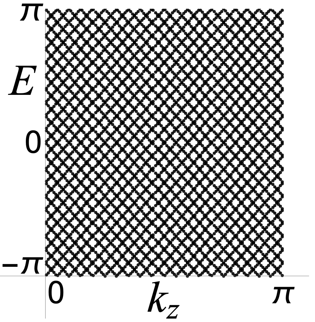
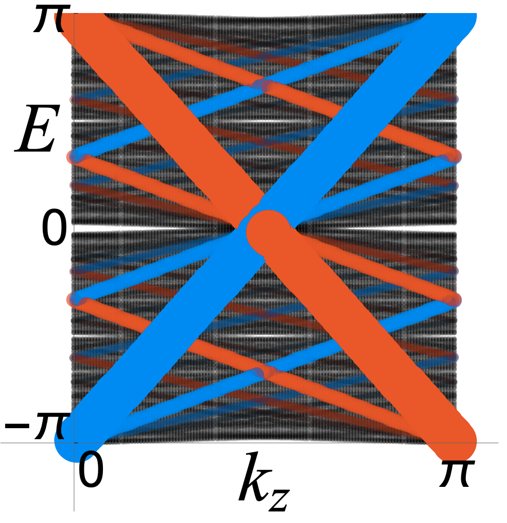
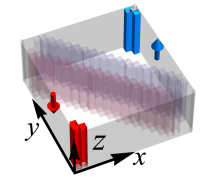
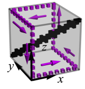
$\frac{\pi}{2}$		4 eigenstates	2 eigenstates
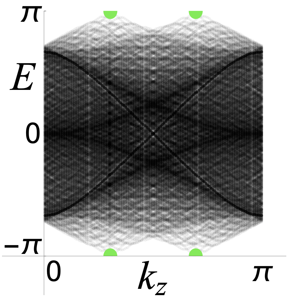
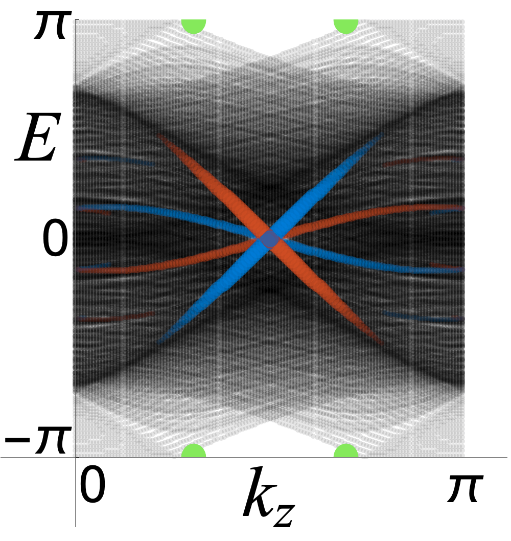
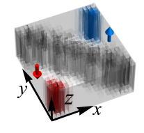
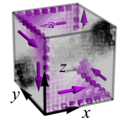
$\frac{\pi}{3}$		3 eigenstates	2 eigenstates
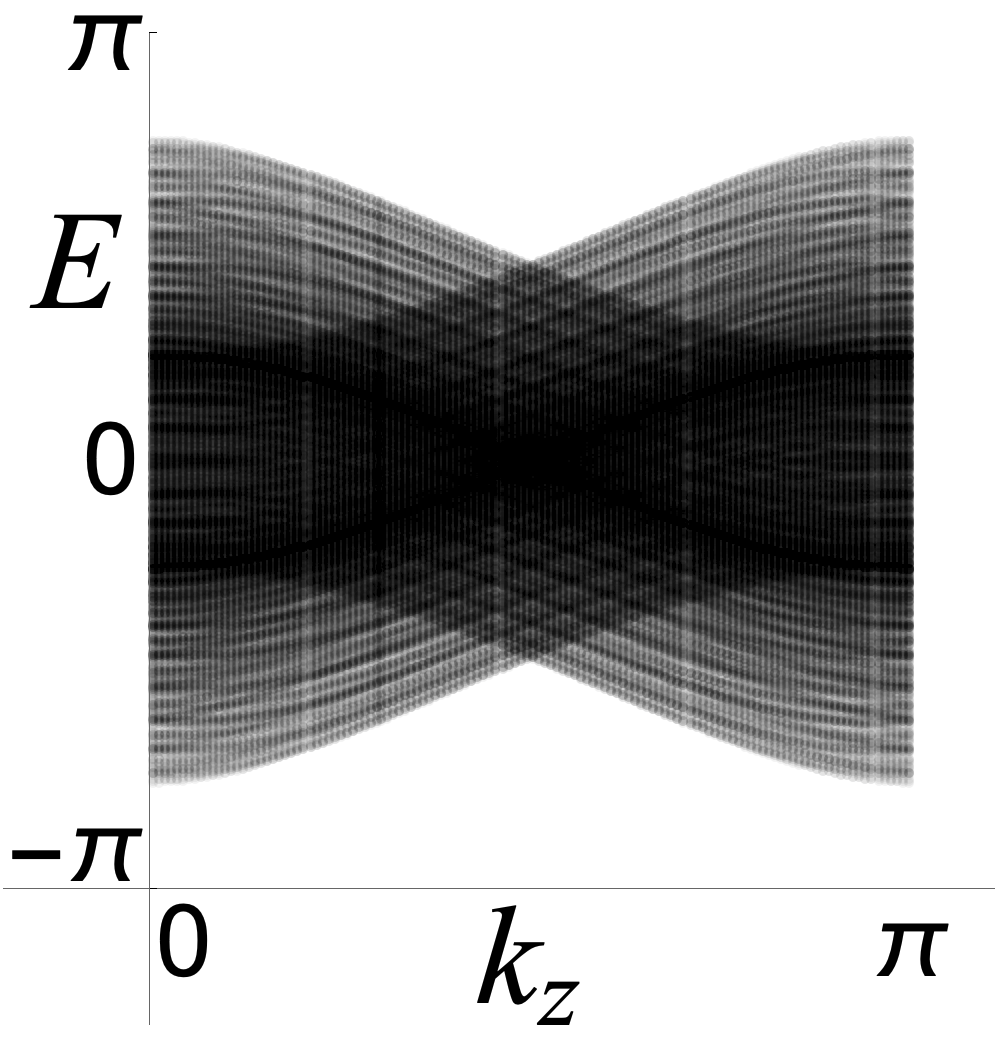
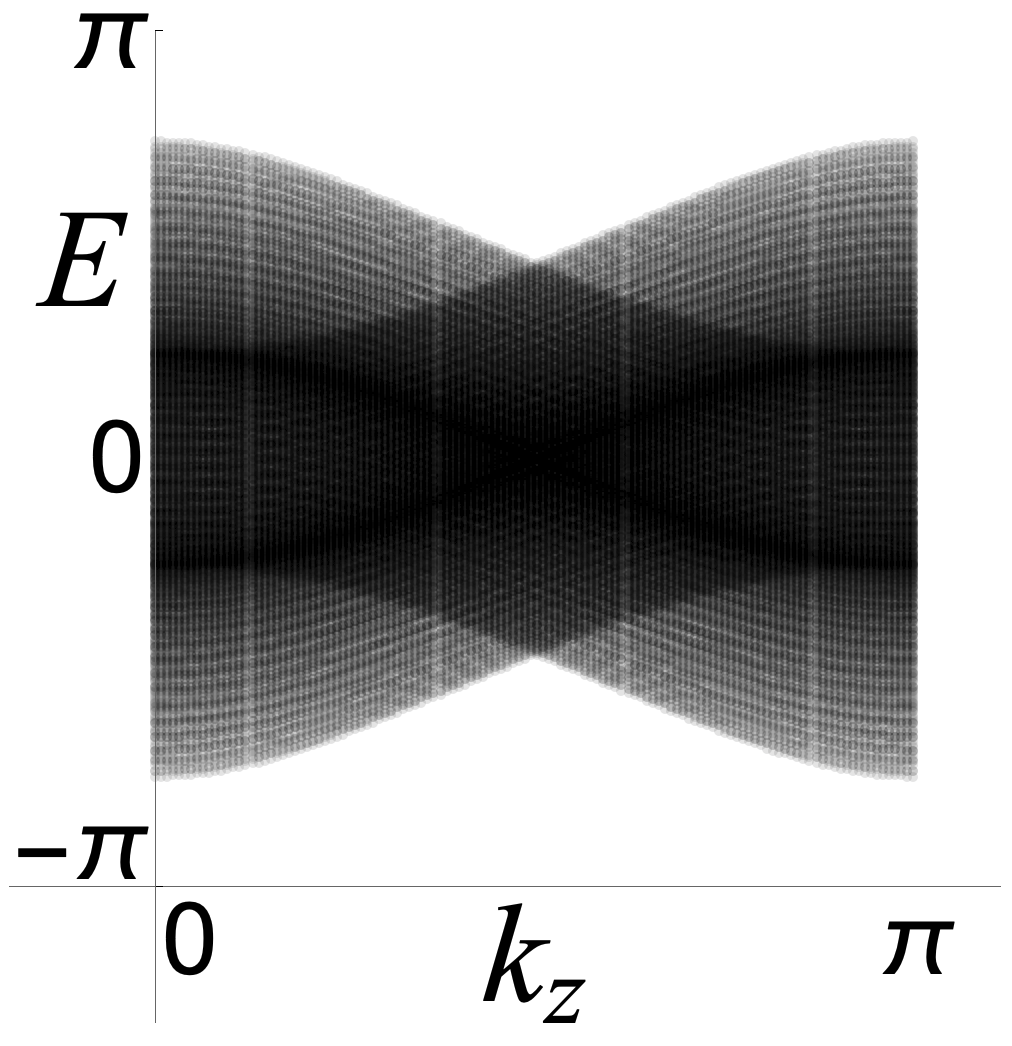
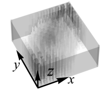
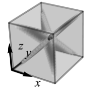
$\frac{\pi}{8}$		1 eigenstate	1 eigenstate

Figure 2: Table showing energy spectra and Floquet modes. The phases of the system are indicated in the vertical axis on the left. The table’s rows refer to the driving parameters $\phi=\pi/8,\pi/3,\pi/2$, corresponding to the metallic phase, the Weyl semimetal/hinge phase, and the fine-tuned point, respectively. The columns represent periodic/open boundary conditions (PBC/OBC) along the specified directions. The system sizes are $L_{x}=L_{y}=40$ in column (1), 20 in (2), and 16 in (3). Columns (1) and (2) contain energy spectra projected onto $k_{z}$. Although the spectra for fully periodic and open boundary conditions in $x$ and $z$ direction are almost identical in the metallic phase ($\phi=\pi/8$), they are very different in the WSM/hinge phase ($\phi=\pi/3$) and at fine tuning ($\phi=\pi/2$). The difference is a result of the formation of chiral hinge modes for open boundary conditions in $x$ and $z$ directions (column 2). This can be inferred also from the dot size reflecting the inverse participation ratio with respect to the site basis as a measure for localization, as well as from the color code indicating the mean distance to two opposite hinges and interpolating from blue for one hinge over black near the center of the system to red for the other hinge. The green dots mark the Weyl points. We also plot the real-space densities of various Floquet modes for open boundary conditions along $x$ and $y$ (column 2) or all (column 3) directions.

III Phase diagram for periodic boundary conditions

$\phi$	Weyl points
$\frac{\pi}{2}$
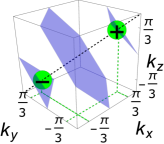
$\frac{\pi}{3}$
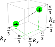
$\frac{\pi}{6}$
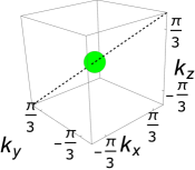
$\frac{\pi}{8}$

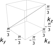
(a) Positions of Weyl points.

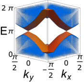
(b) $\phi=\pi/3$, PBC $x,y,z$

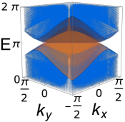
(c) $\phi=\pi/3$, PBC $x,y$

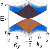
(d) $\phi=\pi/6$, PBC $x,y,z$

Figure 3: (a) The different phases can be distinguished by the presence or absence of Weyl points at quasienergy $\pi$. For $\phi=\pi/8$, in the metallic phase ($\phi<\pi/6$), no Weyl points are present. At the transition, $\phi=\pi/6$, the band touching point appears at $\mathbf{k}=\mathbf{0}$ (green circle). For $\pi/6<\phi<\pi/2$ the band touching splits into two Weyl points of opposite charge (green circles with $\pm$ sign) that separate along the diagonal $k_{x}=-k_{y}=k_{z}$, as shown for $\phi=\pi/3$. At fine tuning $\phi=\pi/2$ the dispersion becomes flat in two directions and the Weyl points disappear to reappear for $\phi>\pi/2$ with reversed charges (signs in green dots correspond to the limit $\phi=\pi/2-0)$. (b-d) Quasienergy spectra versus $k_{x},k_{y}$ for periodic boundary conditions in $x$ and $y$ and either periodic (b,d) or open (c) boundary conditions in $z$ direction. A surface Fermi arc can be observed for $\phi=\pi/3$ by comparing the spectra with periodic (b) and open (c) boundary conditions the $z$ direction. The orange surface denotes the contour formed by quasi-energies closest to $E=\pi$ at each $(k_{x},k_{y})$. For $\phi=\pi/6$ (d) a pair of Weyl points reduces to a single band touching point at the quasi-energy $E=\pi$.

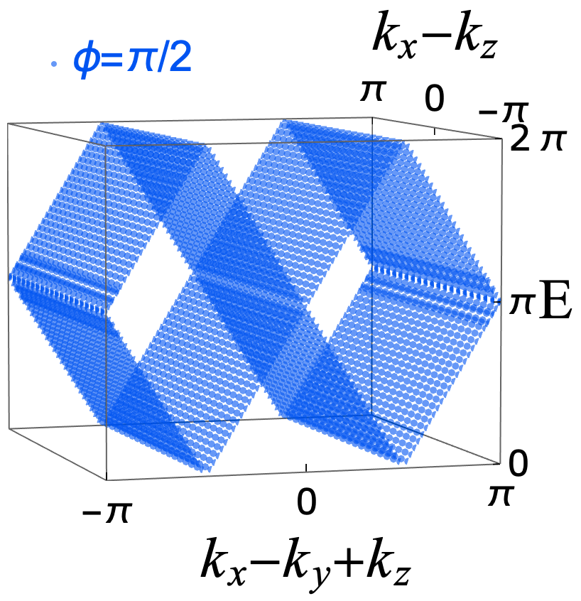
(a) Fine tuned point

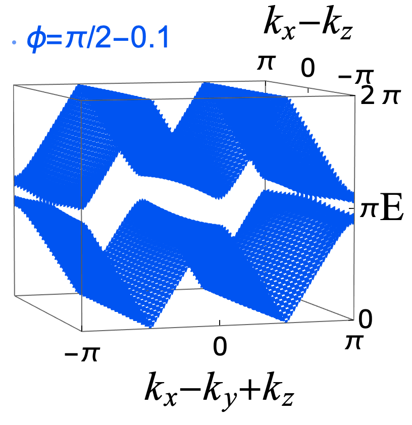
(b) Slight deviation

Figure 4: (a) Anisotropic 1D-like dispersion along the coordinate $k_{x}-k_{y}+k_{z}$ at the fine-tuned point $\phi=\pi/2$. (b) For a small detuning, $\phi=\pi/2-0.1$, the dispersion is no longer completely flat in other two directions, and a pair of non-equivalent Weyl points is formed along the diagonal at $\mathbf{k}=\pm k_{0}(1,-1,1)$. Yet the dispersion remains highly anisotropic.

Before investigating the system with open boundary conditions and the emergence of chiral hinge modes, let us first consider the case of a translation invariant system with periodic boundary conditions. Here, we would focus on the better understood Weyl physics as an anchor point to draw the phase diagram, in order to use it as a reference frame to discuss the new hinge states in the next Section. We clarify that the phase diagram for Weyl physics overlaps, but does not coincide completely with that for the hinge states.

Let us begin with the topologically trivial high-frequency (weak driving) limit corresponding to $\phi\ll 1$. In that case one can retain only the lowest order terms in $\phi$ when expanding the stroboscopic evolution operator $U_{F}$ of Eq. (3), resulting in

$$U_{F}|_{\phi\rightarrow 0}\simeq e^{-i\phi 2(\cos k_{x}+\cos k_{y}+\cos k_{z})\tau_{1}}\,.$$ (6)

The spectrum $\pm 2\phi\sum_{\mu=x,y,z}\cos k_{\mu}$ corresponds to that of a static simple cubic lattice artificially described by 2 sublattices, where the bands are folded as the Brillouin zone size is halved. While the system remains gapless at quasienergy $0$ for arbitrary $\phi$, a characteristic feature of the high-frequency (weak driving) regime is a finite energy gap at quasienergy $\pi$, resulting from the fact that the band width is proportional to $\phi$ and thus is small compared to the dimensionless driving energy $\hbar\omega=2\pi$. This behavior can be observed in the spectrum for $\phi=\pi/8$ shown in Fig. 2 at the bottom of column (1).

Increasing the driving strength $\phi$, the band width grows relative to $2\pi$. When $\phi=\pi/6$ the Floquet band, which is gapless at quasienergy $0$, starts to touch itself at quasienergy $\pi$ and momentum $\mathbf{k}=0$, as one can see in Fig. 3 (d). Going to the regime $\phi\in(\pi/6,\pi/2)$, the band touching point splits into a pair of Weyl points forming at quasienergy $\pi$ with topological charges $\pm 1$, as shown in Fig. 3 (a). They are located at the quasimomenta $\mathbf{k}=k_{0}\mathbf{d}$ along the diagonal vector

$$\mathbf{d}=(1,-1,1),$$ (7)

with

$$k_{0}=\pm\left(1/2\right)\arccos\left[\left(1/2-\sin^{2}\phi\right)/\sin^{2}\phi\right]\,\,\mathrm{modulo}\,\,\pi$$ (8)

(see Appendix A), so that $k_{0}\to\pm\pi/3$ as $\phi\to\pi/2$. We observe the emergence of surface Fermi arc states connecting the Weyl points, when comparing the spectrum with full periodic boundary conditions to that with open boundary conditions along z-direction, as illustrated in Fig. 3 (b) and (c) respectively. Note that the reversed process of increasing driving frequency (or equivalently, decreasing $\phi$ towards $\pi/6$) would correspond to the usual scenario that two Weyl points merge together at $\bm{k}=\bm{0}$ and the spectrum becomes gapped out.

As the driving strength approaches the fine tuned point, $\phi=\pi/2-\varepsilon$ with $\varepsilon\ll 1$, the Weyl dispersion acquires a highly anisotropic form shown in Fig. 4 (b). The dispersion remains steep along the diagonal coordinate $\bm{k}\cdot\mathbf{d}=k_{x}-k_{y}+k_{z}$, but becomes increasingly flat in other two directions. Exactly at fine tuning, $\phi=\pi/2$, the constituent evolution operators (4) reduce to $U_{\mu\pm}\left(\mathbf{k}\right)=-i(\cos k_{\mu}\tau_{1}\pm\sin k_{\mu}\tau_{2})$, and the Floquet stroboscopic operator takes the form $U_{F}=-e^{-i2\tau_{3}\bm{k}\cdot\mathbf{d}}$. This provides the quasi-energies

$$E_{\bm{k},\pm}=\pm 2\bm{k}\cdot\mathbf{d}+(2m+1)\pi\,,$$ (9)

where $m\in\mathbb{Z}$ labels the Floquet bands, and where the upper and lower branches labeled by $\pm$ now directly correspond to sublattices A and B, i.e. $\pm\rightarrow\tau_{3}$. At this fine-tuned point the Weyl points disappear and the dispersion $E_{\bm{k},\pm}$ is completely flat for the momentum plane normal to $\mathbf{d}$, as one can see in Fig. 4 (a). Hence a particle can only propagate along the diagonal $\mathbf{d}$ with a dimensionless velocity $\bm{v_{\pm}}=\pm 2\bm{d}$, depending on whether the particle occupies a site on the sublattice $A$ or $B$ at the beginning of a driving cycle. Note that for fine tuned driving ($\phi=\pi/2$), the Floquet Hamiltonian

$$H_{F}\equiv-i\ln U_{F}=2\tau_{3}\mathbf{d}\cdot\mathbf{k}+\tau_{0}\pi$$ (10)

is periodic in momentum space only thanks to the periodicity in quasi-energies. Such an effective Hamiltonian is characteristic for periodically driven systems, and does not have a static counterpart with finite range hopping.

The fine-tuned dispersion can be understood by considering the dynamics in real space. For $\phi=\pi/2$ in each step $\mu\pm$ the particle is fully transferred from a sublattice A site positioned at $\mathbf{r}_{A}$ to a neighboring site B situated at $\mathbf{r}_{B}=\mathbf{r}_{A}\pm\mathbf{e}_{\mu}$ or vice versa. During the six steps composing the driving period, the particle follows the quasi-one-dimensional trajectory shown in Fig. 1 (b). Thus, after completing each period the particle located on a site of sublattice $A$ ($B$) is transferred by $+2\mathbf{d}$ ($-2\mathbf{d}$) to an equivalent site of the same sublattice, giving rise to stroboscopic motion along the diagonal directions $\pm\mathbf{d}$ at the velocity $\bm{v}_{\pm}$.

Before leaving this Section, we remark that the disappearing of Weyl points at $\phi=\pi/2$ is not because they are gapped out (unlike at $\phi=\pi/6$), but due to the accidental band-gap closure in a whole plane with Weyl points residing on it, as can be seen in Fig. 4 at $\phi=\pi/2$. Consequently there is no need for the two Weyl points to merge at the same location in Brillouin zone when they disappear in this way. More specifically, starting from $\pi/6<\phi<\pi/2$ where Weyl points are well defined, one can enclose a Weyl point with a gapped surface (eigenstates from a certain band) surrounding it, where the Weyl charge is the total Berry flux penetrating out of the surface. At exactly $\phi=\pi/2$, any such surrounding surface would encounter a divergence of local Berry curvature as the two bands become gapless in a whole plane containing the Weyl point and thus are intersecting at any enclosing surfaces. Weyl points and their charges therefore lose definitions at such a fine-tuned point. When the phase $\phi$ exceeds $\pi/2$, the two Weyl points reappear with opposite charges compared to the $\phi<\pi/2$ situation.

IV Chiral hinge modes for open boundary conditions

An intriguing effect shows up when the system is subjected to open boundary conditions with at least two properly chosen boundary planes, where a special type of chiral modes form at certain hinges. In that case eigenstates of the system reorganize into a set states of the quasi-one-dimensional nature orienting parallel to each other and located at various distances from the hinge when open boundaries are introduced. To gain an intuition, it will be useful to start from the fine-tuned point $\phi=\pi/2$ where the stroboscopic motion of the particle at the hinge follows a classical trajectory in real space. Subsequently we will demonstrate numerically the robustness of such chiral hinge modes against parameter changes and inclusion of local defects.

Let us now fix first the notation for later use. We will consider open boundary conditions with a face of a boundary plane oriented perpendicular to a Cartesian axis $\mu=x,y,z$. For full open boundaries the atomic motion is restricted by planes in all three Cartesian directions. We will also investigate a semi-infinite system restricted by two planes orthogonal to $x$ and $y$, while keeping periodic boundary conditions along the $z$ direction. Note that the three-fold symmetry $x\rightarrow y,y\rightarrow z,z\rightarrow-x$ would correspond to shifting the time origin by $T/6$ for the Floquet operator (3), which is merely a gauge transformation and does not change physical observables. Therefore, choosing another combination of open/periodic boundary conditions along different Cartesian directions results in identical phenomena.

Finally, since the boundaries are cut along the orthogonal directions for a cubic lattice, which is not terminating along the directions of Bravais vectors, it is more convenient to label the lattice sites in both sublattices directly by their Cartesian coordinates ${\bm{r}}=(x,y,z)$, with $x,y,z$ taking integer values between $1$ and $L$ carrying units of the lattice constant. The sites belong to the sublattice $A$ (or $B$) for even (or odd) values of $x+y+z$.

IV.1 Fine-tuned driving

IV.1.1 Real-space picture

We will commence our discussion of the hinge dynamics at the fine tuned point using the real space picture. Subsequently in Sec. IV.1.2 we will present a rigorous analysis of the hinge states by going to the momentum representation along the hinge direction. Let us consider the atomic motion for $x\geq 1$ or $y\geq 1$ confined by a single boundary plane at $x=1$ or $y=1$, as illustrated in Fig. 1 (c). Starting from a site deep inside the bulk of, say, sublattice $B$, the particle will propagate stroboscopically on this sublattice covering a distance $-2\bm{d}$ in diagonal direction in each driving period, until approaching the boundary $x=1$ or $y=1$. At the boundary tunneling between the lattice sites $B$ and $A$ cannot occur during one of the six steps of the driving cycle. As a result, the particle changes the sublattice and starts to propagate on the $A$ sublattice in opposite direction. The two colors on each panel of Fig. 1 (c) denote two possible types of such a reflection that are distinguished by the lattice site at which the driving cycle starts leading to the reflection. Specifically a tunneling event is impeded in the first (dark grey) or the fifth (yellow) driving step for a particle situated right at the surface plane $x=1$ ($y=1$) or next to it $x=2$ ($y=2$), as marked by small planes in Fig. 1 (c).

Let us next consider a similar motion of the particle in the region $x\geq 1$ and $y\geq 1$ confined by two intersecting surface planes $x=1$ and $y=1$. After the particle changes the sublattice $B\rightarrow A$ at the $x=1$ boundary, it travels in reversed direction in steps of $2\bm{d}$ until it eventually reaches the $y=1$ surface and is again backreflected, this time with the sublattice change $A\rightarrow B$. In this way, the particle will move back and forth between the $x=1$ and the $y=1$ surfaces which share a hinge.

It is now important to note that each reflection is accompanied by a lateral shift along the surface planes, as can be seen in Fig. 1 (c). Such lateral shifts during reflections resemble the Goos-Hänchen effect occurring when light is reflected at the boundary between two media. The lateral shift would have stronger influence when the particle start from a location closer to the hinge $x=y=1$ or $x=y=L$ where reflections occur more frequently, as illustrated in Fig. 1 (d). In particular, for particles starting from sublattice $B$ at $x=y=1$, the dynamics is completely given by the lateral shift along $-z$ direction, as one can see in the lower part of Fig. 1 (d). The corresponding eigenstate for Floquet operator would be a single chiral mode localized along the hinge propagating along $-z$. Similarly, at $x=y=L$, one can verify that another chiral mode associated with sublattice $A$ propagates along $+z$ direction. Note that these two modes are separated by the whole system size, unlike in the 1D case Budich et al. (2017) with two modes of opposite chirality residing at the same location and thus are subjected to backscattering on imperfections.

In the next Sec. IV.1.2 we will see through rigorous calculation that the whole $xy$-plane can be divided into two parts by an off-diagonal line joining $x=1,y=L$ and $x=L,y=1$, where eigenstates localized closer to $x=y=1$ or $x=y=L$ hinges will carry the chiral motion along $-z$ or $+z$ respectively. Therefore, under perturbations, it will be the eigenstates closest to the center “chirality border line” to lose their chirality along $z$ first, and the hybridization gradually spreads towards the hinges as perturbation strengthens. Importantly, the eigenstates right at the hinges $x=y=1$ and $x=y=L$ do not involve any motion in the $xy$-plane, as can be seen in Fig. 1 (d). They correspond to the genuine chiral hinge modes described by the evolution operator $U_{F}$ over a single period. That means the chirality of such a mode does not depend on the ballistic trajectories finishing several Floquet periods in the $xy$-plane, and thus the closest hinge mode should be more robust against imperfections. This is verified numerically away from fine-tuned point in Fig. 2 (2nd column), and also in Figs. 7 and 8 in the presence of local defects, as will be discussed more specifically later.

Prior to going to a rigorous analytical calculation, we make a side remark regarding the previous Weyl physics. The general boundary reflections exchanging sublattices $A$ and $B$ break particle-hole symmetry $\Gamma=\tau_{3}K$. But that will not destroy the Weyl physics because it reduces the symmetry class from $D$ to $A$, which still hosts a $\mathbb{Z}$ classification for point defect (i.e. Weyl points) in a 3D Brillouin zone Chiu et al. (2016). Furthermore, the orthogonal boundary we choose still preserves the inversion symmetry, and therefore Weyl points and their associated Fermi arcs in the open boundary systems would still exhibit an inversion symmetric fashion as found previously. The only thing that might be slightly affected is the symmetry $E_{1,\bm{k}}=-E_{2,\bm{k}}$ for Fermi arc on the surface, while the Weyl physics phase diagram concerns bulk spectrum and as $L\rightarrow\infty$ surface effects would minimize. The hinge states discussed in this Section do not rely on the particle-hole symmetry either.

IV.1.2 Floquet states

Before carrying out analytical calculations of the Floquet states at the fine-tuned $\phi=\pi/2$, in Figs. 5 and 6 we illustrate the full path of a particle projected onto the $xy$-plane for reflections occurring at $x=1$ and $y=1$ surfaces. One can see in these figures that the particle returns to the same transverse position $(x,y)$ after making two loops. Such a closed trajectory contains two reflections at each boundary $x=1$ and $y=1$, corresponding to the two different types of reflections depicted in Fig. 1(b). The back reflected particle propagates in a trajectory situated closer to the hinge or further away from it for the $B\rightarrow A$ or $A\rightarrow B$ reflections, respectively. This is similar to changing a track for a train before sending it backwards. Because of such chiral Goos-Hänchen shifts, the particle visits a larger number of $B$ sites than $A$ sites when traveling between the two surface planes. Recalling that the ballistic motion over the $B$ or $A$ sites takes place along the diagonal $-\bm{d}$ or $\bm{d}$, the dynamics projected onto the $xy$ place is accompanied by motion in $-z$ or $+z$ direction depending on the sublattice. Thus one arrives at an overall steady advance in $-z$ direction after the particle completes a closed two loop trajectory in the $xy$ plane containing more sites of the $B$ sublattice. Therefore all eigenstates would occupy localized quasi-1D regions in $xy$-plane parallel to each other, each carrying certain group velocity along $z$.

More precisely, as demonstrated in Appendix B, after four reflections by the surfaces, a particle comes back to the original point in the $xy$-plane but shifts by $-2$ units in $z$-direction to an equivalent lattice site. One can similarly verify that a particle comes back to the same $(x,y)$ transverse point after four reflections by the opposite $x=L$ and $y=L$ planes accompanied by a shift by $+2$ lattice unites along $z$ direction.

In this way, the particle’s trajectory starting from any lattice site would roughly covers a quasi-1D region in the $xy$-plane along $\bm{e}_{x}-\bm{e}_{y}$ directions, whose length is proportional to the distance away from the hinge $x=y=1$. All complete double loop trajectories in the $xy$-plane would be associated with a shift by $-2$ or $+2$ along $z$, depending on whether they are closer to the $x=y=1$ or $x=y=L$ hinge. Although such a picture applies to a particle situated further away from the hinges, the advance in the $-z$ or $+z$ direction takes place also for trajectories situated very close to the hinge $x=y=1$ or $x=y=L$ where the particle is reflected simultaneously from both hinge planes, as illustrated in Fig. 1(d) for the $x=y=1$ hinge.

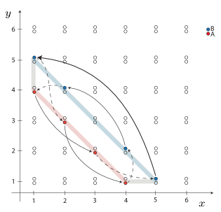
Figure 5: An example of a fine-tuned stroboscopic motion of a particle at the lower-left hinge. The picture shows the projection of the particle’s trajectory in the $xy$ plane. The sites of the $B$ and $A$ sublattices are marked in blue and red, respectively. The particle is initially at the site of the sublattice $B$ characterized by the coordinates $x=M+1$ and $y=1$, with even $M=4$. This corresponds to the lower row ($y=1$) and the fifth column ($x=5$). Subsequently the particle undergoes the stroboscopic evolution described by Eqs. (36)-(42) in Appendix B. Dashed lines with arrows show stroboscopic reflections from the planes $x=1$ or $y=1$. Bulk ballistic trajectories over one/two driving periods are indicated by thin/thick solid arrows. The particle returns to its initial site after $2M+1=9$ periods.

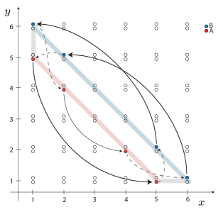
Figure 6: Like in Fig. 5 the particle is initially at the site of the sublattice $B$ with $x=M+1$ and $y=1$, but now with odd $M=5$. The particle returns to the initial site after $2M+1=11$ periods.

The fact that trajectories represent closed loops in the $xy$-plane allows us to construct analytically the eigenstates of the stroboscopic evolution operator $U_{F}$ with open boundaries in $x,y$ and periodic boundary along $z$. The details are elaborated in Appendix B while we outline the results and derivations below. We would chiefly describe the hinge related to $x=y=1$, while mention certain results for $x=y=L$ directly.

Suppose the particle initially occupies a site of the sublattice $B$ with transverse coordinates $y=1$ and $x=M+1$, so the particle is situated at the hinge surface $x=1$ and is $M\geq 0$ sites away from the other $y=1$ hinge surface, as illustrated in Figs. 5 and 6 for $M=4$ and $M=5$. In that case, it takes $2M+1$ driving periods for the particle to come back to the initial position $\left(M+1,1\right)$ in the $xy$ plane, while having shifted by $-2$ lattice units in $z$ direction, i.e.

$$\left(U_{F}\right)^{2M+1}\left|B,M+1,1,z\right\rangle=-\left|B,M+1,1,z-2\right\rangle\,.$$ (11)

After averaging over such a full cycle involving $2M+1$ driving periods, the particle travels with an $M$-dependent mean velocity of $v_{M-}=-2/\left(2M+1\right)$ along the hinge axis $z$ (see Appendix B for more details). Here $|s,x,y,z\rangle$ describes a particle located at site $(x,y,z)$ belonging to sublattice $s=B=-1$ or $s=A=1$ with $s=(-1)^{x+y+z}$.

Let us now consider periodic boundary conditions in $z$ direction with $z=1,2,\dots 2N_{z}$, i.e. $\left|s,x,y,z+2N_{z}\right\rangle=\left|s,x,y,z\right\rangle$, while keeping open boundary conditions in $x$ and $y$. It is then convenient to introduce hybrid position-momentum basis states

$$\left|{s,x,y,k_{z}}\right\rangle^{\prime}=\frac{1}{\sqrt{N_{z}}}\sum_{z}e^{ik_{z}z}\left|s,x,y,z\right\rangle\,.$$ (12)

A basis vector $\left|{s,x,y,k_{z}}\right\rangle^{\prime}$ is characterized by a quasimomenta $k_{z}=m\pi/N_{z}$ with $m=0,1,\dots,N_{z}-1$, where $k_{z}$ is defined modulo $\pi$, as the lattice periodicity equals to 2 length units in $z$ direction. Equation (11) yields

$$\left(U_{F}\right)^{2M+1}\left|{B,M+1,1,k_{z}}\right\rangle^{\prime}=-\left|{B,M+1,1,k_{z}}\right\rangle^{\prime}e^{2ik_{z}}\,.$$ (13)

The above results are for a particle starting from the hinge surface $y=1,x=M+1$, which traces out a closed loop for its classical trajectory visiting $2M+1$ sites at different stroboscopic moments. In a similar manner, if the particle starts at any intermediate site of the trajectory at stroboscopic moment $pT$,

$$\left|M,k_{z},p\right\rangle\equiv\left(U_{F}\right)^{p}\left|{B,M+1,1,k_{z}}\right\rangle^{\prime}\,,$$ (14)

it will also finish the loop after $2M+1$ driving periods:

$$\left(U_{F}\right)^{2M+1}\left|M,k_{z},p\right\rangle=-\left|M,k_{z},p\right\rangle e^{2ik_{z}}\,,$$ (15)

with $p=0,1,\ldots 2M$. By superimposing the states $\left|M,k_{z},p\right\rangle$ corresponding to all sites involved in the stroboscopic trajectory, one can construct the Floquet hinge states representing eigenstates of the Floquet evolution operator $U_{F}$:

$$\overline{\left|M,k_{z},q\right\rangle}=\frac{1}{\sqrt{2M+1}}\sum_{p=0}^{2M}\left|M,k_{z},p\right\rangle\exp\left(\mathrm{i}\frac{2\pi q-2k_{z}+\pi}{2M+1}s\right)\,,$$ (16)

where the index $q=0,1,\ldots,2M$ labels these modes. The corresponding quasienergies for the eigenstates (16) situated closer to the $x=y=1$ reads

$$E_{M,k_{z},q}=\left(\frac{2\pi q-2k_{z}+\pi}{2M+1}\right)\textrm{ mod }2\pi\,.$$ (17)

An analogous dispersion but with an opposite slope (opposite sign for the group velocity along $z$) can be obtained for the states formed closer to the opposite hinge $x=y=L$. The dispersion branches for both types of hinge modes reproduce the spectrum shown in the row 1 and column (2) of Fig. 2. The corresponding eigenstates are quasi-1D in $xy$-plane along $\bm{e}_{y}-\bm{e}_{x}$ and are plane-waves along $z$.

Such a spectrum of the system with open boundary conditions in $x$ and $y$ directions looks completely different from the one for full periodic boundary conditions shown in column (1) of Fig. 2 or Fig. 4 (a), where in the latter case all the bulk modes have the same positive or negative dispersion slope (group velocity) $v_{z}=\pm 2$. In contrast, for the beam geometry [column (1) of Fig. 2] the spectrum is now organized into Eq. (17), representing different quasi-1D eigenstates $M$ sites away from the hinge $x=y=1$. Each eigenstate is characterized by a different group velocity

$$v_{M\pm}=\pm\frac{2}{2M+1}$$ (18)

decreasing with the distance $M$ from the hinge, where “$-$” and “$+$” correspond to the states located relatively closer to $x=y=1$ and $x=y=L$ respectively. The red / blue colors in Fig. 2 indicate the mean distance of each mode from the two relevant hinges. The dark red (blue) mode associated with $M=0$ is localized directly at the hinge $x=y=1$ ($x=y=L$) and propagates at the largest velocity in negative (positive) $z$ direction. Modes with a smaller slope have larger $M$ and thus are located further away from the particular hinge, as indicated by the color. The real-space density of four different hinge modes at $\phi=\pi/2$ is illustrated in the real-space plot shown in row 1 and column (2) of Fig. 2. In addition, a measure for the degree of localization of a mode $|\psi\rangle$ is the inverse participation ratio $\text{IPR}=\sum_{j}|\langle j|\psi\rangle|^{4}$, with real-space site states $|j\rangle$ and the Floquet eigenstates $|\psi\rangle$. It is shown in the spectra of Fig. 2 via the dot size roughly indicating the inverse of the number of sites a mode is spread over. Thus modes localized near the hinges have larger IPR than those that are more spread over in $xy$-plane locating further away from the hinges, indicating that the latter modes with smaller chiral group velocities are less narrowly localized in $xy$-plane than the former faster modes located closer to the hinge.

In this way, the group velocity $v_{M\pm}$ along the $z$ direction with open boundaries along $x,y$ is very different from the projected group velocity $v_{z}=\mathbf{v}\cdot\mathbf{e}_{z}$ of a full periodic system. This is due to the unidirectional bulk group velocity $\mathbf{v}=\pm 2\mathbf{d}$ and can be intuitively understood as follows. Each eigenstate of the system with open boundary conditions involves 4 boundary reflections, as can be inferred from Figs. 5 and 6. Such an eigenstate is composed of two pairs of counterpropagating plane waves representing the eigenstates of the original periodic system propagating along the cubic diagonal $\pm\bm{d}$ with the $z$ projection of the group velocity $v_{z}=\pm 2$. Consequently the original group velocity in the bulk gets neutralized, and the overall group velocity $v_{M\pm}$ along $z$ is due to the combined Goos-Hänchen shift over 4 times of boundary reflections. As the Goos-Hänchen process occurs more frequently near the hinges $x=y=1$ and $x=y=L$, the magnitude of group velocity $v_{M,\pm}=\pm 2/(2M+1)$ is maximum at the hinges for $M=0$, while close to the central part where $M\propto L$, the group velocity $v_{M\pm}$ becomes rather small, and eventually vanishes in the thermodynamic limit $v_{M\pm}\propto 1/L\rightarrow 0$. This is quite different from a usual crystal where modes closer to the center of the bulk should be more insensitive to any boundary effects, while in our case one arrives at another situation where $v_{z}=\pm 2$ for the periodic boundary conditions while for open boundary conditions one has $v_{M\pm}\rightarrow 0$ for the modes near the bulk center.

The observation that the whole (Floquet) spectrum and the corresponding eigenstates of our system are completely reorganized, when switching from periodic to open boundary conditions, resembles the extensive accumulation of boundary modes featured in the non-Hermitian skin effect Yao and Wang (2018); Bergholtz et al. (2020); Ashida et al. (2020); Kawabata et al. (2020). Therefore, the formation of an extensive number of reconstructed chiral hinge modes in our Floquet system might be called chiral second-order Floquet skin effect, in analogy to the terminology used for non-Hermitian systems Kawabata et al. (2020). A subtle difference is that the eigenstates of a unitary Floquet evolution operator are orthogonal to each other, unlike eigenstates of non-Hermitian Hamiltonians that that are generally non-orthogonal. It implies the counting rule that on average, there can be at most one Floquet eigenstate per lattice site, so an accumulation of states right at the boundary is not possible in a Floquet system. Note also that the non-Hermitian skin effect is associated with the exceptional points of the non-Hermitian Hamiltonian when the boundaries are introduced Bergholtz et al. (2020); Ashida et al. (2020), whereas no exceptional points are formed for periodically driven systems described by the unitary Floquet evolution operators. More details on these issues are available in Appendix C.

IV.2 Beyond fine-tuned driving

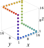
(a) without defect

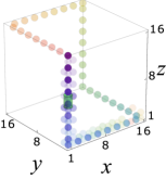
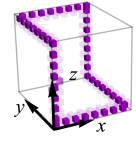
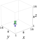
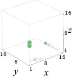
(b) with defect
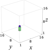
(c1) $t=3$ (c2) $t=5$ (c3) $t=20$

Figure 7: The dynamics of a particle initially localized at the site $(x,y,z)=(1,1,16)$ for a system of $16\times 16\times 16$ sites with full open boundary conditions and fine tuned $\phi=\pi/2$. The squared wave function at different times is reflected in the opacity of the plotted dots. Different colors indicate time. (a) Without defect. (b) In the presence of a potential defect of energy $\Delta=3\pi$ at the two sites marked by the green tube. Additionally, we plot the squared wave function of one hinge mode. (c) Snapshots of the time evolution in the presence of the defect at different times.

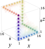
(a) without defect

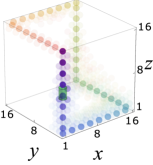
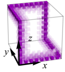
(b) with defect

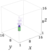
(c1) $t=3$

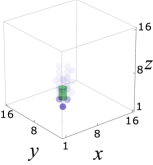
(c2) $t=5$

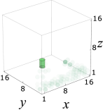
(c3) $t=20$

Figure 8: As Fig. 7, but for $\phi=0.9\times\pi/2$, away from fine tuning.

Although the above analysis is based on ballistic trajectories at the fine-tuned driving parameter $\phi=\pi/2$, we expect the chirality of the hinge modes to be robust also against perturbations and tuning away from $\phi=\pi/2$. This applies especially to the hinge states with larger chiral velocities, which are situated closer to the hinge and thus are spatially well separated from counter-propagating modes at the opposite hinge. The chiral hinge modes persist for a rather wide range of $\phi$ beyond $\phi=\pi/2$. This can be observed from the example of $\phi=\pi/3$ ($33.3\%$ detuning, half-way across the Weyl phase transition) displayed in Fig. 2 column (2) around $k_{z}=\pi/2$ and $E=0$. We can see that the hinge modes at smaller distances $M$ from the hinge still preserve their chirality along the hinge, as expected previously. In turn, hinge modes with larger $M$ that are closer to the sample center, are gradually mixed with modes of opposite chirality and lose chiral nature together with localization in the $xy$-plane when $\phi$ deviates away from $\phi=\pi/2$.

We have also considered the exemplary eigenstates for a cube geometry with full open boundary conditions along all Cartesian axes $x$, $y$ and $z$ presented in column (3) of Fig. 2 showing that for $\phi=\pi/2$ and $\phi=\pi/3$ the chiral modes at certain hinges are joined to form a closed loop respecting inversion symmetry of the system [see also Fig. 7 (a)]. The six hinges not participating in this closed loop do not carry hinge modes, since their two boundary planes are not connected along the diagonal direction $\bm{d}$. Meanwhile, non-hinge modes representing the bulk dynamics all center along the cubic diagonal [column (3) of Fig. 2].

In the previous Sections we have made arguments that at the fine tuning, $\phi=\pi/2$, the chiral modes locating right at the hinge $x=y=1$ (or $x=y=L$) do not involve the ballistic motion in the $xy$-plane over many driving periods, and therefore their chiral transporting feature should be preserved even if they become hybridized with nearby modes carrying different or no chirality. We now further test such an expectation by checking the robustness of chiral hinge transports in the presence of local defects in Figs. 7 and 8. Here, we simulate the dynamics of a particle in the presence of a defect for a system with open boundary conditions in all three directions representing a generalization of the defect-free situation shown in column (3) of Fig. 2. Figure 7 illustrates the dynamics of a particle initially located at a corner $(x,y,z)=(1,1,16)$ of the system, where two orthogonally oriented transporting hinges meet, (a) for the fine tuned situation without a defect and (b) in the presence of a strong potential offset of $\Delta=3\pi$ on two neighboring hinge sites (indicated by a green tube) at $(x,y,z)=(1,1,8),(1,1,9)$, respectively. The corresponding plots for non-fine-tuned driving with $\phi=0.9(\pi/2)$ are presented in Fig. 8. We find that despite this strong defect the chiral nature of the hinge modes ensures that no backscattering occurs at the defect and the majority of the wave-packet continues to follow chiral trajectories along the hinges. In Figs. 7 (b) and 8 (b) we also plot representative eigenstates of the system with defects. These eigenstates remain localized at the hinge, with only a small distortion compared to the situation without defect shown in column (3) of Fig. 2. That means the localization properties of the particle carrying the chiral motion along the hinge are not just an ephemeral phenomena. Once the original particle distribution overlaps with such an eigenstate, certain portion of those particles will always be localized along the hinge undergoing constant chiral motion. This is further verified in Fig. 9 for evolution over a long time. It shows the time-evolved state after 100 driving cycles for the non-fine-tuned system ($\phi=0.9\times\pi/2$) both without defect (a) and with defect (b). Very similar distribution is also found after even longer evolution, e.g. over 1000 driving cycles; the densities are, thus, representative for late-time states in the limit $t\to\infty$. Note that such a process implies the particle have encountered the defects for many (or infinite) times when they loop over the connected hinges repeatedly, without losing their localization the hinge and being scattered away.

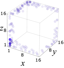
(a) $\Delta=0$

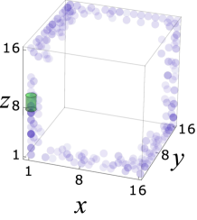
(b) $\Delta=3\pi$

Figure 9: Density distribution of a particle initially localized at the corner site $(x,y,z)=(1,1,16)$ after an evolution over $100$ driving cycles for the non-fine-tuned parameter $\phi=0.9\times\pi/2$, without defect (a) and with a defect (b) [corresponding to the parameters of Fig. 8 (b)]. The densities are representative for late-time states in the limit $t\to\infty$ as similar distribution is found also after 1000 driving cycles.

steps	1	2	3	4	5	6
$\alpha_{00}$	0	0	0	1	1	1
$\alpha_{10}$	1	0	1	0	1	0
$\alpha_{01}$	1	1	0	0	0	1
$\alpha_{11}$	0	1	1	1	0	0

$$\text{<img src="/html/2101.08281/assets/fig4\_scheme.png" id="S4.F10.5.1.m1.1.1.g1nest" class="ltx\_graphics ltx\_img\_square" width="150" height="153" alt="Refer to caption">}1$$ $$\text{<img src="/html/2101.08281/assets/fig4\_scheme2.png" id="S4.F10.6.2.m2.1.1.g1nest" class="ltx\_graphics ltx\_img\_square" width="150" height="153" alt="Refer to caption">}2$$

$$\text{<img src="/html/2101.08281/assets/fig4\_scheme3.png" id="S4.F10.7.3.m1.1.1.g1nest" class="ltx\_graphics ltx\_img\_square" width="150" height="155" alt="Refer to caption">}3$$ $$\text{<img src="/html/2101.08281/assets/fig4\_scheme4.png" id="S4.F10.8.4.m2.1.1.g1nest" class="ltx\_graphics ltx\_img\_square" width="150" height="158" alt="Refer to caption">}4$$

$$\text{<img src="/html/2101.08281/assets/fig4\_scheme5.png" id="S4.F10.9.5.m1.1.1.g1nest" class="ltx\_graphics ltx\_img\_square" width="150" height="159" alt="Refer to caption">}5$$ $$\text{<img src="/html/2101.08281/assets/fig4\_scheme6.png" id="S4.F10.10.6.m2.1.1.g1nest" class="ltx\_graphics ltx\_img\_square" width="150" height="157" alt="Refer to caption">}6$$

Figure 10: The stepwise modulation of the dimensionless superlattice amplitudes $\alpha_{ab}$ according to the protocol given in the table, gives rise to different dimerizations of the cubic lattice in each driving step, that enables tunneling along the desired bonds.

V Experimental Realization with ultracold atoms in optical lattices

V.1 Engineering of the driven lattice

Above, we have shown that the proposed modulation of tunneling gives rise to a variety of phenomena, including the robust creation of a pair of Weyl points, unidirectional bulk transport, chiral Goos-Hänchen-like shifts, and the macroscopic accumulation of chiral hinge modes for open boundary conditions corresponding to a chiral second-order Floquet skin effect. The model itself is, nevertheless, rather simple and its implementation with ultracold atoms in optical lattices can be accomplished using standard experimental techniques. All what is needed is a static cubic host lattice potential of equal depth $V_{0}$ in each Cartesian direction and a superlattice potential, whose amplitudes along various diagonal lattice directions are modulated in a stepwise fashion in time in order to suppress/allow tunneling along the six different bonds specified by our protocol. This can be achieved using the following optical lattice potential:

$$V(\bm{r})=V_{0}\sum_{\mu=x,y,z}\cos^{2}(2k_{L}r_{\mu})$$

$$+V_{1}\sum_{a,b=0,1}\alpha_{ab}(t)\cos^{2}k_{L}(x+(-1)^{a}y+(-1)^{b}z)\,,$$ (19)

where only two of the four modulating lasers $\alpha_{ab}$ with $a,b=0,1$ are turned on in each driving step, as shown in Fig. 10. Such a modulation provides the required six-stage driving of the cubic lattice. Note that a similar modulation has recently been implemented in two dimensions Wintersperger et al. (2020).

V.2 Detection of hinge dynamics

To observe the dynamics associated with the hinge modes, one can apply the boxed potential achieved in recent experiments Gaunt et al. (2013); Navon et al. (2016); Mukherjee et al. (2017b); Lopes et al. (2017a, b); Eigen et al. (2017); Ville et al. (2018). There, thin sheets of laser beams penetrate through the quantum gases creating a steep potential barrier. Three pairs of such beams are imposed in a three-dimensional system, creating the sharp “walls” for the box potential while leaving the central part of the gases homogeneous.

Essentially, such a potential combined with our lattice driving scheme immediately leads to the particle dynamics described in Fig. 7 and Fig. 8. To take into account realistic experimental situations, two modifications are adopted in our following simulations. First, we consider the effect of a relatively “softer” wall for the box potential with

$$V_{\text{box}}(\bm{r})=\frac{V_{b}}{2}\sum_{\mu=x,y,z}\left(2+\tanh\frac{r_{\mu}^{(1)}-r_{\mu}}{\xi}+\tanh\frac{r_{\mu}-r_{\mu}^{(2)}}{\xi}\right),$$ (20)

where the potential ramps up over a finite distance of roughly $4\xi$ near the boundaries $r_{\mu}^{(1,2)}$, see Fig. 11 for instance. The second modification we adopt is that the initial state is not taken to be localized on a single lattice site but described by a gaussian wave packet of finite width,

$$\psi_{i=(x,y,z)}(t=0)=e^{-[(x-x_{0})^{2}+(y-y_{0})^{2}+(z-z_{0})^{2}]/2s_{0}^{2}}.$$ (21)

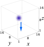
(a) $|\psi_{i}(t=0)|$

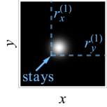
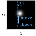
(b) Projection to $x$-$y$ (left) and $x$-$z$ (right)

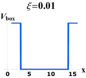
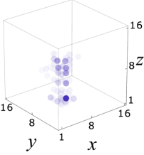
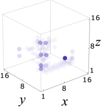
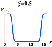
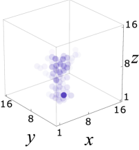
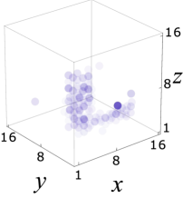
(c1) Ideal boundary (c2) $|\psi_{i}(t=5)|$ (c3) $|\psi_{i}(t=10)|$   (d1) Softer boundary (d2) $|\psi_{i}(t=5)|$ (d3) $|\psi(t=10)|$

Figure 11: The dynamics of particles in a box potential with different softness of the boundary. The initial density distribution takes a Gaussian profile spreading over several lattice sites. The parameters are $\phi=\pi/2,V_{b}T/6\hbar=7.5\pi$. The initial Gaussian profile has the center $(x_{0},y_{0},z_{0})=(4,4,12)$ and width $s_{0}=0.75$.

The results of the dynamics are presented in Fig. 11 (c1)–(c3) and (d1)–(d3), for the ideal sharp boundary (as in Fig. 7) and the realistic softer boundaries in experimental setting respectively. We see that the chiral motion snapshots for the ideal/softer boundaries exhibit qualitatively the same characters, signaling that a softer boundary does not cause significant changes. This is in consistent with the previous simulation showing the robustness of hinge states and their resulting chiral dynamics against local defects in Fig. 7 and Fig. 8. The major difference from previous cases, then, derives from the initial state that overlaps with more than one set of eigenstates near the hinge, each with different group velocities as given in Eq. (18). Finally, we mention that some portion of initial particle distribution would reside within the region with significant changes in $V_{\text{box}}$. That portion of the particles could be permanently confined to the initial hinge due to a mechanism similar to Wannier-Stark localization. However, the majority of the particles are still traveling into the connecting hinges, as shown in Fig. 11 (c3) and (d3).

In cold atom experiments, the density profiles are usually detected by taking a certain projection plane, where the integrated (column-averaged) densities are observed. To this end, we point out that the hinge dynamics can be confirmed by observing the density profiles in two perpendicular planes. A schematic plot is given in Fig. 11 (b), corresponding to the dynamics along the hinge $x=y\sim 1$. The density profile taken at $x-y$ plane (i.e. the “top” view) would show a localized distribution at the corner, verifying the particles only locate at $x=y\sim 1$. Meanwhile, the profile at $x-z$ plane (i.e. “side” view) indicates the movement/spreading along $z$. In a more general situation, i.e. at long time limit with all 6 hinges populated as in Fig. 9, additional image projection planes could be exploited. We also mention that a simultaneous implementation of multiple imaging planes have been applied in experiments Lu et al. (2020); Wang et al. .

V.3 Detection of Floquet Weyl points

Weyl physics has been explored in recent cold atom experiments and theoretical proposals Lu et al. (2020); Wang et al. ; Zhang et al. (2015); Dubček et al. (2015); He et al. (2016), and also extensively in solid state systems Armitage et al. (2018). Here, we discuss a scheme closely related to a recent experiment Ünal et al. (2019); Wintersperger et al. (2020) detecting the spacetime singularities in anomalous Floquet insulators.

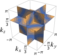
(a1) $\Delta^{(0)}$ at $\phi=\pi/8$

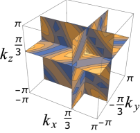
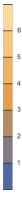
(a1) $\Delta^{(0)}$ at $\phi=\pi/3$

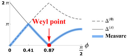
(b) Exemplary gap at $\bm{k}_{0}=k_{0}(1,-1,1)$ with $k_{0}=\pi/3-0.2$.

Figure 12: Simulation of gap measurements using Stückelberg interferometry. (a1) and (a2) Contours for quasi-energy gap at $E=0$, for $\phi=\pi/8$ and $\phi=\pi/3$ respectively. (b) The gaps at $E\sim 0$ and $E\sim\pi$, and the measured gap which takes the smaller one of the two.

First, the band touching at Weyl points can be verified using the Stückelberg interferometry Zenesini et al. (2010); Kling et al. (2010); Shevchenko et al. (2010); Wintersperger et al. (2020). Such a method measures the smaller gap for the two bands at $E\sim 0$ and $\pi$, see Ref. Wintersperger et al. (2020) for details. Compared with the experiments for insulators, a difference here is that the two bands are, overall, always gapless at $E=0$. That means if a global gap is measured, it will prevent us from gaining information about the gaps or band touching at quasienergy $E=\pi$. But fortunately, there exists a finite region neighboring to $\bm{k}_{0}=\pi/3(1,-1,1)$ where the bands are always gapped at $E=0$ for all $\phi$, see Fig. 12 (a1), (a2) for example. Then a local gap closure can be measured near $\bm{k}_{0}$.

The specific measurement for our case can be performed in the following way. An example for $\bm{k}_{0}=(\pi/3-0.2)(1,-1,1)$ is presented in Fig. 12 (b). Let us denote the quasi-energy of the two Floquet bands at $\bm{k}_{0}$ with $E_{\pm}(\bm{k}_{0})=\pm E_{0}$. Here, we use the branch cut along $\pi$ in taking the logarithm of Floquet eigenvalues $e^{-iE_{\pm}(\bm{k}_{0})}$. They have the same magnitudes and opposite signs due to particle-hole and inversion symmetry as explained in Sec. II. Then, the local gap around $E\sim 0$ is $\Delta^{(0)}\equiv 2E_{0}$, while the other gap around the Floquet Brillouin zone boundary $E\sim\pi$ is $\Delta^{(\pi)}\equiv 2\pi-2E_{0}$. Therefore, $\Delta^{(0)}=\Delta^{(\pi)}$ can only occur at $0,\pi$ mod $2\pi$. In experiments, one can start from the high frequency limit ($\phi\rightarrow 0$) where the band width is small compared to $2\pi$ and therefore the measured gap always corresponds to $\Delta^{(0)}$. Slowing down the driving, the gap $\Delta^{(\pi)}$ shrinks while the other gap $\Delta^{(0)}$ expands. At some point, the two gaps coincide with their magnitudes, as shown in Fig. 12 (b). Since it is always the smaller one of $\Delta^{(0)}$ and $\Delta^{(\pi)}$ that will show up in experimental measurement, one will observe a cusp shape of the measured gap, i.e. near $\phi\approx 0.41$ in Fig. 12 (b). One could then imply from the occurrence of the cusp that for $\phi>0.41$, the experimental data starts to reveal $\Delta^{(\pi)}$, whose vanishing at $\phi\approx 0.87$ shows the existence of the Weyl point around $E\sim\pi$. Similar measurements can be performed for $\bm{k}$ slightly deviating from $\bm{k}_{0}$, which will show that at $\phi=0.87$, $\Delta^{(\pi)}$ remains finite, proving that the band closure around $E\sim\pi$ is a point contact. When the designated $\phi$ is slowly approached, one can perform a measurement of the gap at a certain $\bm{k}$. A shortcut for our system is that focusing on quasimomenta along the diagonal $\bm{k}_{0}=k_{0}(1,-1,1)$ is sufficient to determine the Weyl point, as discussed in Sec.III.

With the Weyl points determined, one could further apply band tomography Hauke et al. (2014); Fläschner et al. (2016) method for momentum states surrounding a certain Weyl point in order to determine its charge. Note that one does not need the eigenstate information throughout the whole Brillouin zone as the two bands are gapless in certain regions, except for just an arbitrarily small surface wrapping a Weyl point $\bm{k}^{\text{(Weyl)}}$ determined previously. As shown before, near the Weyl points in our model, there exists a finite region where the two bands are fully gapped in both $E\sim 0$ and $\pi$, which allows for populating eigenstates with bosons at a certain band Fläschner et al. (2016); Wintersperger et al. (2020). As an example, in Fig. 13 (a) we illustrate the surfaces formed by 6 faces $q_{x,y,z}=\pm 0.5$ of a cube, where $\bm{q}=\bm{k}-\bm{k}^{(\text{Weyl})}$, with $\bm{k}^{(\text{Weyl})}\approx 0.955\times(1,-1,1)$ for $\phi=\pi/3$, as in Fig. 2. From the full information of the Floquet eigenstates $|u_{n,\bm{k}}\rangle$ given by Eq. (5), the Berry curvature penetrating out of a plane normal to the unit vector $\bm{e}_{\mu}$ can be computed as $\Omega_{\mu}(\bm{k})=\pm i\sum_{\nu\rho}\varepsilon_{\mu\nu\rho}\left(\langle\partial_{k_{\nu}}u_{n,\bm{k}}|\partial_{k_{\rho}}u_{n,\bm{k}}\rangle\right)$, where $\varepsilon_{\mu\nu\rho}$ is the Levi-Civita symbol, and $\pm$ sign denotes that the unit vector penetrating out of the cube is along $\pm\bm{e}_{\mu}$ directions. Figure 13 shows momentum resolved Berry curvatures in each wrapping surface and their net fluxes $\int_{\text{surf}}d\bm{k}\Omega_{\mu}(\bm{k})$ in that plane.

(a) The surfaces wrapping a Weyl point

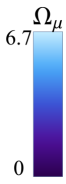
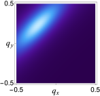
(b1) $\Omega_{z+}$, net 1.284

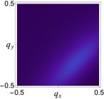
(b2) $\Omega_{z-}$, net 0.866

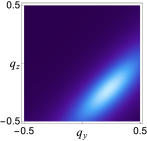
(b3) $\Omega_{x+}$, net 1.284

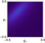
(b4) $\Omega_{x-}$, net 0.866

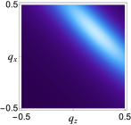
(b5) $\Omega_{y+}$, net 1.469

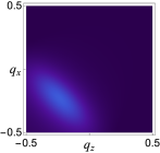
(b6) $\Omega_{y-}$, net 0.513

Figure 13: The Berry curvatures for the surfaces wrapping a Weyl point. Adding the net Berry curvatures up we have $2\pi$.

VI Conclusion

In this paper, we have shown that three-dimensional periodically driven lattice systems can experience a complete reconstruction of its eigenstates with drastically different features, when subjected to open boundary conditions. This corresponds to a chiral second-order Floquet skin effect. An intuitive understanding of this effect was given by considering the system at a fine-tuned point of the periodic driving, where the bulk motion can only take place forwards or backwards along a single diagonal direction. As a consequence, for open boundary conditions, the particle is reflected back and forth between hinge-sharing surface planes, indicating a combination of counter-propagating original bulk eigenstates carrying opposite group velocity into new chiral Floquet states associated with the hinge. Thus the original bulk motion becomes neutralized, while the new group velocities are associated with a Goos-Hänchen shift during boundary reflections, which are most significant close to hinges where the particles is reflected more frequently.

This effect offers a alternative mechanism to generate hinge modes in addition to the more well-understood cases such as (Floquet) higher-order topological phases. The robustness of the chiral hinge modes here is more relevant to the special dispersion characteristic of Floquet systems, which allows for all eigenstates to be localized in a quasi-one-dimensional region close to fine-tuned point, while not necessarily require a bulk gap. While we briefly discuss in Appendix D a topological quantity specific to the fine-tuned point $\phi=\pi/2$, it will be an interesting future direction to explore whether such chiral hinge modes would have a stable and rigorous topological nature. The previous analysis Titum et al. (2016) have shown that the requirement of bulk quasi-energy gap becomes less important to characterize topologically protected chiral modes (i.e. Fig. 4 (a) (ii) in Titum et al. (2016)). While weak disorder could mix different momentum states and destroy the hinge modes, it will be interesting to see whether a set of more robust hinge modes would emerge in the strongly disordered regime where all modes are localized, and to check the possible crossover or transitions when one increases the disorder strengths. Our current approach and discussions would also be useful for considering observable effects in experiments, similar to the case of Weyl semimetals where surface defects/disorder would partly destroy the Fermi arc but the chiral transport will be partially preserved therein Wilson et al. (2018).

It is noteworthy that even modes close to bulk center suffer from a complete reconstruction by open boundaries, hosting very different group velocity in the thermodynamic limit. Such an effect resembles the accumulation of boundary modes in systems described by a non-hermitian Hamiltonian. Yet different from this non-Hermitian skin effect, in our system we can have at most one state per lattice site on average, as Floquet states are orthogonal to each other. Thus in our system the accumulation corresponds to the emergence of hinge-bound modes at increasing distance from the hinge. Another interesting aspect is the competition or interplay between the hinge modes and the emergence of robust Wely points in our system, so the hinge states can co-exist with the Fermi arc surface states. The implementation of the model featuring both the second-order Floquet skin effect and the Weyl physics is straightforward with ultracold atoms in optical superlattices.

VII Acknowledgment

The authors thank E. Anisimovas and F. Nur Ünal for helpful discussions. We acknowledge funding by the European Social Fund under grant No. 09.3.3-LMT-K-712-01-0051 and the Deutsche Forschungsgemeinschaft (DFG) via the Research Unit FOR 2414 under Project No. 277974659.

Appendix A Evolution operator and quasienergies along the diagonal

A.1 Evolution operator

In the bulk the stroboscopic evolution operator $U_{F}$ is generally given by Eqs. (3)-(4) in the main text. Let us consider the operator $U_{F}$ for wave-vectors $\mathbf{k}$ along the cubic diagonal direction $\bm{d}=(1,-1,1)$, for which

$$\bm{k}=k_{0}\bm{d}\quad\text{and, thus,}\quad|\bm{k}|=\sqrt{3}|k_{0}|\,.$$ (22)

In that case Eqs. (3)-(4) simplify to

$$U_{F}=\left[U\left(k_{0}\right)U\left(-k_{0}\right)\right]^{3}\,,$$ (23)

where

$$U\left(k_{0}\right)=\tau_{0}\cos\phi-\mathrm{i}\tau_{k_{0}}\sin\phi\,,$$ (24)

with $\tau_{k_{0}}=\tau_{1}\cos{k_{0}}+\tau_{2}\sin{k_{0}}$, where $\tau_{1,2,3}$ are Pauli matrices for the sublattice freedom, $\tau_{0}$ being a unit $2\times 2$ matrix. Explicitly one, thus, has

$$U\left(k_{0}\right)U\left(-k_{0}\right)=\left[\cos^{2}\phi-\sin^{2}\phi\cos\left(2k_{0}\right)\right]\tau_{0}+\mathrm{i}b\,,$$ (25)

with

$$b=\sin^{2}\phi\sin\left(2k_{0}\right)\tau_{3}-\sin(2\phi)\cos k_{0}\tau_{1}.$$ (26)

A.2 Quasi-energies

The evolution operator $U_{F}=e^{-\mathrm{i}H_{F}}$ defines the quasienergies representing the eigenvalues of the of the Floquet Hamiltonian $H_{F}$, which describes the stroboscopic time evolution in multiples of the driving period $T=1$. Using Eqs. (23) and (25) for the evolution operator, one arrives at the following equation for the quasi-energies $E_{\mathbf{k}}$

$$\cos\left(E_{\mathbf{k}}/3\right)=\cos^{2}\phi-\sin^{2}\phi\cos\left(2k_{0}\right)\,.$$ (27)

This provides the dispersion (modulo $2\pi$) along the diagonal $k_{x}=-k_{y}=k_{z}=k_{0}$

$$E_{k_{0}\bm{d},\gamma}=3\gamma\arccos\left[\cos^{2}\phi-\sin^{2}\phi\cos\left(2k_{0}\right)\right],\,\,\mathrm{with}\,\,\gamma=\pm 1\,.$$ (28)

In particular, quasienergies $E_{k_{0}\bm{d},\gamma}=\pi$ (modulo $2\pi$) correspond to

$$\cos^{2}\phi-\sin^{2}\phi\cos\left(2k_{0}\right)=1/2\,,$$ (29)

and thus

$$\cos\left(2k_{0}\right)=\frac{1/2-\sin^{2}\phi}{\sin^{2}\phi}\,,$$ (30)

giving (modulo $\pi$)

$$k_{0}=\pm\left(1/2\right)\arccos\left[\left(1/2-\sin^{2}\phi\right)/\sin^{2}\phi\right]\,.$$ (31)

At the fine tuned point ($\phi=\pi/2$) the condition Eq.(29) reduces to

$$\cos\left(2k_{0}\right)=-1/2\,,\quad\mathrm{giving}\quad k_{0}=\pm\pi/3\,.$$ (32)

On the other hand, at $\phi=\pi/6$ one has $\sin^{2}\phi=1/4$, so that

$$\cos\left(2k_{0}\right)=1,\,\quad\mathrm{giving}\quad k_{0}=0\,.$$ (33)

In this way, two band touching points are formed at quasienergy $\pi$ for $\pi/6<\phi<\pi/2$, as well as for $\pi/2<\phi<5\pi/6$ (beyond the fine tuning point at $\phi=\pi/2$). By taking $\phi<\pi/6$ or $\phi>5\pi/6$, Eq.(29) can no longer be fulfilled, so a band gap is formed at quasienergy $\pi$.

Appendix B Stroboscopic hinge motion at fine tuning

In this Appendix we give a detailed description of the stroboscopic real-space dynamics of the system at fine tuning, $\phi=\pi/2$, giving rise to chiral hinge-bound Floquet modes. We will consider the hinge that is shared by the two surface planes oriented in the $-x$ and $-y$ direction, which is parallel to the $z$-axis. The projection of the particle’s trajectory in the $xy$ plane is illustrated in Figs. 5 and 6. A particle of sublattice $s=+1,-1\equiv A,B$ is translated by $2s\bm{d}$ during each driving cycle, provided $x+2s\geq 1$ and $y-2s\geq 1$ to ensure it does not hit any the boundary plane. In that case the state-vector $\left|s,x,y,z\right\rangle$ transforms according to the following rule after a single driving period:

$$U_{F}\left|s,x,y,z\right\rangle=-\left|s,x+2s,y-2s,z+2s\right\rangle\,.$$ (34)

The particle thus propagates with a stroboscopic velocity $\mathbf{v}=2s\left(1,-1,1\right)$ in opposite directions $s=\pm 1$ for different sublattices $A$ and $B$.

Suppose initially the particle occupies a site of the sublattice $B$ at the boundary $y=1$ situated $M$ sites away from the hinge ($x=M+1$) with odd $M+z$, so that $s=B=-1$. The corresponding initial state vector is $\left|s,M+1,1,z\right\rangle\equiv\left|B,M+1,1,z\right\rangle$. The subsequent stroboscopic trajectory projected to the $xy$ plane is shown in Fig. 5 for $M=4$ and in Fig. 6 for $M=5$. Generally it takes $\left(2M+1\right)$ driving periods for the system to return to its initial state $\left|M+1,1,z\right\rangle$. To see this, consider the stroboscopic evolution of the particle with an even $M>2$ and odd $z$. The stroboscopic motion of the particle then splits into four bulk and four boundary segments illustrated in Fig. 5 for $M=4$.

During the first $M/2$ driving periods the particle undergoes the bulk ballistic motion along the sites of the $B$ sublattice, and the state vector transforms as $\left|B,M+1,1,z\right\rangle\rightarrow\left|B,1,M+1,z-M\right\rangle$. Subsequently the particle is reflected from the plane $x=1$ to a site of the sublattice $A$ situated closer to the hinge, $\left|B,1,M+1,z-M\right\rangle\rightarrow\left|A,2,M-1,z+2-M\right\rangle$, as shown in Fig. 1(c) of the main text. During the next $M/2-1$ driving periods the particle propagates ballistically along the sites of the $A$ sublattices, giving $\left|A,2,M-1,z+2-M\right\rangle\rightarrow\left|A,M,1,z\right\rangle$. The subsequent reflection from the plane $y=1$ brings the particle to a site of the $B$ sublattice situated further away to from the hinge, $\left|A,M,1,z\right\rangle\rightarrow\left|B,M,2,z-2\right\rangle$. The evolution takes place in the similar way during final four segments. Explicitly the full stroboscopic dynamics is given by:

$$\left(U_{F}\right)^{M/2}\left|B,M+1,1,z\right\rangle=\left(-1\right)^{M/2}\left|B,1,M+1,z-M\right\rangle\,,$$ (35)

$$U_{F}\left|B,1,M+1,z-M\right\rangle=-\mathrm{i}\left|A,2,M-1,z+2-M\right\rangle\,,$$ (36)

$$\left(U_{F}\right)^{M/2-1}(-\mathrm{i})\left|A,2,M-1,z+2-M\right\rangle$$

$$=\mathrm{i}\left(-1\right)^{M/2}\left|A,M,1,z\right\rangle\,,$$ (37)

$$U_{F}\mathrm{i}\left|A,M,1,z\right\rangle=\left|B,M,2,z-2\right\rangle\,,$$ (38)

$$\left(U_{F}\right)^{M/2-1}\left|B,M,2,z-2\right\rangle=-\left(-1\right)^{M/2}\left|B,2,M,z-M\right\rangle\,,$$ (39)

$$U_{F}(-1)\left|B,2,M,z-M\right\rangle=\mathrm{i}\left|A,1,M,z-M\right\rangle\,,$$ (40)

$$\left(U_{F}\right)^{M/2-1}\mathrm{i}\left|A,1,M,z-M\right\rangle$$

$$=(-\mathrm{i})\left(-1\right)^{M/2}\left|A,M-1,2,z-2\right\rangle\,,$$ (41)

$$U_{F}(-\mathrm{i})\left|A,M-1,2,z-2\right\rangle=-\left|B,M+1,1,z-2\right\rangle\,,$$ (42)

In this way, after $\left(2M+1\right)$ driving periods the particle returns back to the initial position $\left(M+1,1\right)$ in the $xy$ plane and is shifted by $2$ lattice units to an equivalent point of the sublattice $B$ in the direction opposite to the $z$ axis. The same holds for the initial state vector $\left|B,M+1,1,z\right\rangle$ characterized by an odd $M$ and even $z$ (see Fig. 6 for $M=5$), as well as for a particle situated closer to the hinge ($0\leq M\leq 3$) where the reflections can take place simultaneously from both planes $x=1$ and $y=1$, as illustrated in Fig. 1(d) in the main text. Thus one can write for any distance $M\geq 0$ from the hinge:

$$\left(U_{F}\right)^{2M+1}\left|B,M+1,1,z\right\rangle=-\left|B,M+1,1,z-2\right\rangle\,,$$ (43)

This means the particle propagates along the hinge in the $-z$ direction with the stroboscopic velocity equal to $-2/\left(2M+1\right)$. The relations analogous to Eq.(43) hold for all $2M+1$ states of the stroboscopic sequence featured in Eqs. (36)-(42)

The origin of such chiral hinge states can be explained as follows. The particle in the sublattice $B$ is reflected to a site of the $A$ sublattice situated closer to the hinge, whereas the particle in the sublattice A is reflected to a site of the sublattice $B$ situated further away from the hinge, as one can see in Figs. 5 and 6, as well as in Eqs. (36), (38), (40), (42). Consequently the number of $B$ sites visited over all $2M+1$ driving periods ($M+1$) exceeds the corresponding number of $A$ sites ($M$). The four reflections do not yield any total shift of the particle in the $z$ direction. On the other hand, the ballistic motion between sites the same sublattice $B$ ($A$) is accompanied by a shift by $2$ lattice sites in the $z$ ($-z$) direction for each driving period. This leads to the overall shift of the particle to an equivalent site in the $-z$ direction is due to the difference in the number of the visited $B$ and A sites after $2M+1$ driving periods.

Appendix C Non-Hermitian Hamiltonian corresponding to stroboscopic operator

Recently it was suggested Bessho and Sato (2020) to associate a non-Hermitian Hamiltonian $H_{NH}\left(\mathbf{k}\right)$ to the momentum space stroboscopic evolution operator $\mathrm{i}U_{F}\left(\mathbf{k}\right)$. Let us consider such a non-Hermitian Hamiltonian for our 3D periodically driven lattice

$$H_{NH}=\mathrm{i}U_{F}\,.$$ (44)

For the fine tuned driving ($\phi=\pi/2$) the bulk stroboscopic evolution operator corresponds to a non-Hermitian Hamiltonian describing a unidirectional transfer between the lattice sites along the diagonal $\mathbf{d}=(1,-1,1)$ and in the opposite direction $-\mathbf{d}$ for the sublattices $A$ and $B$, respectively:

$$H_{NH}^{bulk}=-\mathrm{i}\sum_{\mathbf{r}_{A}}\left|A,\mathbf{r}_{A}+2\mathbf{d}\right\rangle\left\langle A,\mathbf{r}_{A}\right|-\mathrm{i}\sum_{\mathbf{r}_{B}}\left|B,\mathbf{r}_{B}-2\mathbf{d},\right\rangle\left\langle B,\mathbf{r}_{B}\right|\,.$$ (45)

The open boundary conditions for the hinge corresponding to $x\geq 1$ and $y\geq 1$ are obtained by imposing a constraint on the state-vectors entering the real space non-Hermitian Hamiltonian (45)

$$\left|s,\mathbf{r}_{s}\right\rangle=0\quad\mathrm{for}\quad\mathbf{r}_{s}\cdot\mathrm{e}_{x,y}\leq 0,\,\,\mathrm{with}\,\,s=A,B\,.$$ (46)

The bulk non-Hermitian Hamiltonian (45) supplied with the open boundary conditions (46) describes a unidirectional coupling between unconnected linear chain of the $A$ or $B$ sites terminating at the hinge planes. The eigenstates of each linear chain represent non-Hermitian skin modes which are localized at one end of the chain depending on the direction of asymmetric hopping Bergholtz et al. (2020); Ashida et al. (2020). In the present situation such skin modes would be trivially localised on different planes of the hinge for the chains comprising different sublattice sites $A$ or $B$, and no chiral motion is obtained along the hinge.

Yet the open boundary conditions (46) are not sufficient to properly represent the boundary behavior of a particle in our periodically driven lattice. In fact, bulk non-Hermitian Hamiltonian (45) supplied with the boundary conditions (46) is no longer a unitary operator. Thus one can not associate such an non-Hermitian operator with the evolution operator, in contradiction with Eq. (44). The unitarity is restored by adding to $H_{NH}^{bulk}$ extra terms [in addition to the conditions (46)] to include effects of the chiral backward reflection at the hinge planes to a neighboring linear chain composed of the sites of another sublattice. These terms are described by Eqs.(36), (38), (40) and (42), and correspond to the dashed lines in Figs. 5-6. The chiral reflection appears due to the micromotion during the driving period involving six steps (see Fig. 1(b)), and is a characteristic feature of the periodically driven 3D lattice. As discussed in the previous Appendix B, the backreflection leads to the chiral motion along the hinge.

Appendix D Tentative discussions on topological origins

An interesting question is whether the robust chiral hinge states are a consequence of topological properties of the driven system. However, as we see from column (2) of Fig. 2, the quasi-energies of hinge states are fully mixed with the bulk spectrum, and therefore no traditional topological band theories for gapped or semimetallic systems apply. Here, we apply an approach similar to that used in refs. Kitagawa et al. (2010) and Budich et al. (2017) for computing topological invariant at a fine-tuned parameter point, where eigenstates are analytically obtainable, and a topological invariant based on eigenstate projections can be calculated.

In section IV.1 we have obtained equation (15) describing the evolution over $2M+1$ driving periods of the $M$th hinge state $\left|M,k_{z},p\right\rangle$ at the fine tuned point. Using this equation one can define the the quasienergy winding number Kitagawa et al. (2010) for the $M$th hinge state via the Floquet evolution operator over the $2M+1$ driving periods:

$$W_{M}=\frac{1}{2\pi i}\int_{0}^{\pi}dk_{z}U_{k_{z},2M+1}^{-1}\partial_{k_{z}}U_{k_{z},2M+1}=1\,,$$ (47)

where

$$U_{k_{z},2M+1}=\left\langle M,k_{z},p\right|\left(U_{F}\right)^{2M+1}\left|M,k_{z},p\right\rangle=-e^{2ik_{z}}\,,$$ (48)

with $p=0,1,\ldots 2M$. In Eq. (47) the integration over $k_{z}$ extends over one Brillouin zone of width $\pi$, as the distance between two non-equivalent lattice sites equals to $2$ in $z$ direction. A similar procedure can be applied to the opposite hinge at $(x,y)=(L,L)$, where the hinge modes shown in blue in column (2) of Fig. 2 are characterized by the opposite group velocity and thus the winding number is opposite $W_{M}=-1$.

The rigorous quantization of the topological invariant $W_{M}$ is associated with the fine tuning, $\phi=\pi/2$. However, the spatial separation between hinge modes of opposite chirality allows to preserve their chiral character also away from the fine tuning point $\phi=\pi/2$, as one can see in column (2) of Fig. 2. Thus, the formation of bulk states via the mixing of hinge modes of opposite chirality happens mostly in the center of the system, where hinge modes corresponding to large $M$ and small chiral velocities lie close by to their counter propagating partners associated with the opposite hinge. In turn, the states with the largest chiral velocity, which are situated close to the hinge and far away from counter-propagating modes of the opposite hinge, are much less affected by a small detuning.

In this way, tuning away from $\phi=\pi/2$ we find a crossover (rather than a topological transition) in which the chiral hinge modes are gradually destroyed, as can be observed in the real-space plots in columns (2) and (3) of Fig. 2. Note that already a small deviation from the fine tuned point $\phi=\pi/2$ destroys the chiral hinge states in a narrow region near $k_{z}=0$ and $E=\pi$, as can be seen from the spectrum shown for $\phi=\pi/3$ in column (2) of Fig. 2. In this spectral surface Fermi arc states are formed, which equally provide definite chiral transport, yet around the surfaces rather than the hinges. Thus a fraction of the chiral hinge states is transformed into Fermi arc surface states in the vicinity of the Weyl points. The latter states extend to a larger and larger spectral area as the detuning increases.

References

- Kitagawa et al. (2010) T. Kitagawa, E. Berg, M. Rudner, and E. Demler, Phys. Rev. B 82, 235114 (2010).
- Rudner et al. (2013) M. S. Rudner, N. H. Lindner, E. Berg, and M. Levin, Phys. Rev. X 3, 031005 (2013).
- Roy and Harper (2017a) R. Roy and F. Harper, Phys. Rev. B 96, 155118 (2017a).
- Yao et al. (2017a) S. Yao, Z. Yan, and Z. Wang, Phys. Rev. B 96, 195303 (2017a).
- Mukherjee et al. (2017a) S. Mukherjee, A. Spracklen, M. Valiente, E. Andersson, P. Öhberg, N. Goldman, and R. R. Thomson, Nat. Commun. 8, 13918 (2017a).
- Peng et al. (2016) Y.-G. Peng, C.-Z. Qin, D.-G. Zhao, Y.-X. Shen, X.-Y. Xu, M. Bao, H. Jia, and X.-F. Zhu, Nat. Commun. 7, 13368 (2016).
- Maczewsky et al. (2016) L. J. Maczewsky, J. M. Zeuner, S. Nolte, and A. Szameit, Nat. Commun. 8, 13756 (2016).
- von Keyserlingk and Sondhi (2016) C. W. von Keyserlingk and S. L. Sondhi, Phys. Rev. B 93, 245145 (2016).
- Else and Nayak (2016) D. V. Else and C. Nayak, Phys. Rev. B 93, 201103 (2016).
- Potirniche et al. (2017) I.-D. Potirniche, A. C. Potter, M. Schleier-Smith, A. Vishwanath, and N. Y. Yao, Phys. Rev. Lett. 119, 123601 (2017).
- Wintersperger et al. (2020) K. Wintersperger, C. Braun, F. N. Ünal, A. Eckardt, M. D. Liberto, N. Goldman, I. Bloch, and M. Aidelsburger, Nat. Phys. 16, 1058 (2020).
- Sacha (2015) K. Sacha, Phys. Rev. A 91, 033617 (2015).
- Khemani et al. (2016) V. Khemani, A. Lazarides, R. Moessner, and S. L. Sondhi, Phys. Rev. Lett. 116, 250401 (2016).
- Else et al. (2016) D. V. Else, B. Bauer, and C. Nayak, Phys. Rev. Lett. 117, 090402 (2016).
- Yao et al. (2017b) N. Y. Yao, A. C. Potter, I.-D. Potirniche, and A. Vishwanath, Phys. Rev. Lett. 118, 030401 (2017b).
- Zhang et al. (2017) J. Zhang, P. Hess, A. Kyprianidis, P. Becker, A. Lee, J. Smith, G. Pagano, I.-D. Potirniche, A. C. Potter, A. Vishwanath, et al., Nature 543, 217 (2017).
- Choi et al. (2017) S. Choi, J. Choi, R. Landig, G. Kucsko, H. Zhou, J. Isoya, F. Jelezko, S. Onoda, H. Sumiya, V. Khemani, et al., Nature 543, 221 (2017).
- Rovny et al. (2018) J. Rovny, R. L. Blum, and S. E. Barrett, Phys. Rev. Lett. 120, 180603 (2018).
- Ho et al. (2017) W. W. Ho, S. Choi, M. D. Lukin, and D. A. Abanin, Phys. Rev. Lett. 119, 010602 (2017).
- Huang et al. (2018) B. Huang, Y.-H. Wu, and W. V. Liu, Phys. Rev. Lett. 120, 110603 (2018).
- Sacha and Zakrzewski (2017) K. Sacha and J. Zakrzewski, Rep. Prog. Phys. 81, 016401 (2017).
- Yao and Nayak (2018) N. Yao and C. Nayak, Phys. Today 71, 40 (2018).
- Sacha (2020) K. Sacha, Time Crystals (Springer International Publishing, Switzerland, 2020).
- von Keyserlingk et al. (2016) C. W. von Keyserlingk, V. Khemani, and S. L. Sondhi, Phys. Rev. B 94, 085112 (2016).
- Benalcazar et al. (2017a) W. A. Benalcazar, B. A. Bernevig, and T. L. Hughes, Science 357, 61 (2017a).
- Benalcazar et al. (2017b) W. A. Benalcazar, B. A. Bernevig, and T. L. Hughes, Phys. Rev. B 96, 245115 (2017b).
- Khalaf (2018) E. Khalaf, Phys. Rev. B 97, 205136 (2018).
- Yan et al. (2018) Z. Yan, F. Song, and Z. Wang, Phys. Rev. Lett. 121, 096803 (2018).
- Wang et al. (2018) Q. Wang, C.-C. Liu, Y.-M. Lu, and F. Zhang, Physical Review Letters 121, 186801 (2018).
- Huang and Liu (2020) B. Huang and W. V. Liu, Phys. Rev. Lett. 124, 216601 (2020).
- Peng and Refael (2018) Y. Peng and G. Refael, Phys. Rev. Lett. 123, 016806 (2018).
- Bomantara et al. (2019) R. W. Bomantara, L. Zhou, J. Pan, and J. Gong, Phys. Rev. B 99, 045441 (2019).
- Rodriguez-Vega et al. (2019) M. Rodriguez-Vega, A. Kumar, and B. Seradjeh, Phys. Rev. B 100, 085138 (2019).
- Plekhanov et al. (2019) K. Plekhanov, M. Thakurathi, D. Loss, and J. Klinovaja, Physical Review Research 1, 032013 (2019).
- Yao and Wang (2018) S. Yao and Z. Wang, Phys. Rev. Lett. 121, 086803 (2018).
- Bergholtz et al. (2020) E. J. Bergholtz, J. C. Budich, and F. K. Kunst, “Exceptional topology of non-hermitian systems,” (2020), arXiv:1912.10048 [cond-mat.mes-hall] .
- Ashida et al. (2020) Y. Ashida, Z. Gong, and M. Ueda, “Non-hermitian physics,” (2020), arXiv:2006.01837 [cond-mat.mes-hall] .
- Kawabata et al. (2020) K. Kawabata, M. Sato, and K. Shiozaki, Phys. Rev. B 102, 205118 (2020).
- Wu et al. (2019) H. C. Wu, L. Jin, and Z. Song, Phys. Rev. B 100, 155117 (2019).
- Xiao et al. (2020) L. Xiao, T. Deng, K. Wang, G. Zhu, Z. Wang, W. Yi, and P. Xue, Nature Physics 16, 761 (2020).
- Song et al. (2019) F. Song, S. Yao, and Z. Wang, Physical Review Letters 123, 170401 (2019).
- Budich et al. (2017) J. C. Budich, Y. Hu, and P. Zoller, Phys. Rev. Lett. 118, 105302 (2017).
- Armitage et al. (2018) N. Armitage, E. Mele, and A. Vishwanath, Rev. Mod. Phys. 90, 015001 (2018).
- Anderson et al. (2012) B. M. Anderson, G. Juzeliūnas, V. M. Galitski, and I. B. Spielman, Phys. Rev. Lett. 108, 235301 (2012).
- Anderson et al. (2013) B. M. Anderson, I. B. Spielman, and G. Juzeliūnas, Phys. Rev. Lett. 111, 125301 (2013).
- Dubček et al. (2015) T. Dubček, C. J. Kennedy, L. Lu, W. Ketterle, M. Soljačić, and H. Buljan, Phys. Rev. Lett. 114, 225301 (2015).
- Sun et al. (2018) X.-Q. Sun, M. Xiao, T. c. v. Bzdušek, S.-C. Zhang, and S. Fan, Phys. Rev. Lett. 121, 196401 (2018).
- Higashikawa et al. (2019) S. Higashikawa, M. Nakagawa, and M. Ueda, Phys. Rev. Lett. 123, 066403 (2019).
- Lu et al. (2020) Y.-H. Lu, B.-Z. Wang, and X.-J. Liu, Science Bulletin 65, 2080 (2020).
- (50) Z.-Y. Wang, X.-C. Cheng, B.-Z. Wang, J.-Y. Zhang, Y.-H. Lu, C.-R. Yi, S. Niu, Y. Deng, X.-J. Liu, S. Chen, and J.-W. Pan, 2004.02413v1 .
- (51) Y. Zhu, T. Qin, X. Yang, G. Xianlong, and Z. Liang, 2003.05638v2 .
- Lang et al. (2017) L.-J. Lang, S.-L. Zhang, K. T. Law, and Q. Zhou, Phys. Rev. B 96, 035145 (2017).
- Note (1) Without including the tunneling along the direction described by third and the sixth driving steps, the dynamics reduces to a 2D motion in a periodically driven square lattice considered in refs. Rudner et al. (2013); Mukherjee et al. (2017a); Wintersperger et al. (2020).
- Altland and Zirnbauer (1997) A. Altland and M. R. Zirnbauer, Phys. Rev. B 55, 1142 (1997).
- Chiu et al. (2016) C.-K. Chiu, J. C. Teo, A. P. Schnyder, and S. Ryu, Rev. Mod. Phys. 88, 035005 (2016).
- Roy and Harper (2017b) R. Roy and F. Harper, Phys. Rev. B 96, 155118 (2017b).
- Gaunt et al. (2013) A. L. Gaunt, T. F. Schmidutz, I. Gotlibovych, R. P. Smith, and Z. Hadzibabic, Phys. Rev. Lett. 110, 200406 (2013).
- Navon et al. (2016) N. Navon, A. L. Gaunt, R. P. Smith, and Z. Hadzibabic, Nature 539, 72 (2016).
- Mukherjee et al. (2017b) B. Mukherjee, Z. Yan, P. B. Patel, Z. Hadzibabic, T. Yefsah, J. Struck, and M. W. Zwierlein, Phys. Rev. Lett. 118, 123401 (2017b).
- Lopes et al. (2017a) R. Lopes, C. Eigen, A. Barker, K. G. Viebahn, M. R. de Saint-Vincent, N. Navon, Z. Hadzibabic, and R. P. Smith, Phys. Rev. Lett. 118, 210401 (2017a).
- Lopes et al. (2017b) R. Lopes, C. Eigen, N. Navon, D. Clément, R. P. Smith, and Z. Hadzibabic, Phys. Rev. Lett. 119, 190404 (2017b).
- Eigen et al. (2017) C. Eigen, J. A. Glidden, R. Lopes, N. Navon, Z. Hadzibabic, and R. P. Smith, Phys. Rev. Lett. 119, 250404 (2017).
- Ville et al. (2018) J. L. Ville, R. Saint-Jalm, E. Le Cerf, M. Aidelsburger, S. Nascimbène, J. Dalibard, and J. Beugnon, Phys. Rev. Lett. 121, 145301 (2018).
- Zhang et al. (2015) D.-W. Zhang, S.-L. Zhu, and Z. D. Wang, Phys. Rev. A 92, 013632 (2015).
- He et al. (2016) W.-Y. He, S. Zhang, and K. T. Law, Phys. Rev. A 94, 013606 (2016).
- Ünal et al. (2019) F. N. Ünal, B. Seradjeh, and A. Eckardt, Phys. Rev. Lett. 122, 253601 (2019).
- Zenesini et al. (2010) A. Zenesini, D. Ciampini, O. Morsch, and E. Arimondo, Phys. Rev. A 82, 065601 (2010).
- Kling et al. (2010) S. Kling, T. Salger, C. Grossert, and M. Weitz, Phys. Rev. Lett. 105, 215301 (2010).
- Shevchenko et al. (2010) S. N. Shevchenko, S. Ashhab, and F. Nori, Phys. Rep. 492, 1 (2010).
- Hauke et al. (2014) P. Hauke, M. Lewenstein, and A. Eckardt, Phys. Rev. Lett. 113, 045303 (2014).
- Fläschner et al. (2016) N. Fläschner, B. Rem, M. Tarnowski, D. Vogel, D.-S. Lühmann, K. Sengstock, and C. Weitenberg, Science 352, 1091 (2016).
- Titum et al. (2016) P. Titum, E. Berg, M. S. Rudner, G. Refael, and N. H. Lindner, Phys. Rev. X 6, 021013 (2016).
- Wilson et al. (2018) J. H. Wilson, J. H. Pixley, D. A. Huse, G. Refael, and S. D. Sarma, Physical Review B 97, 235108 (2018).
- Bessho and Sato (2020) T. Bessho and M. Sato, “Topological duality in floquet and non-hermitian dynamical anomalies: Extended nielsen-ninomiya theorem and chiral magnetic effect,” (2020), arXiv:2006.04204 [cond-mat.mes-hall] .