PRINCIPAL COMPONENT ANALYSIS FOR ESTIMATING PARAMETERS OF THE L1287 DENSE CORE BY FITTING MODEL SPECTRAL MAPS INTO OBSERVED ONES

Abstract

An algorithm has been developed for finding the global minimum of a multidimensional error function by fitting model spectral maps into observed ones. Principal component analysis is applied to reduce the dimensionality of the model and the coupling degree between the parameters, and to determine the region of the minimum. The $k$–nearest neighbors method is used to calculate the optimal parameter values. The algorithm is used to estimate the physical parameters of the contracting dense star-forming core of L1287. Maps in the HCO⁺(1–0), H¹³CO⁺(1–0), HCN(1–0), and H¹³CN(1–0) lines, calculated within a 1D microturbulent model, are fitted into the observed ones. Estimates are obtained for the physical parameters of the core, including the radial profiles of density ($\propto r^{-1.7}$), turbulent velocity ($\propto r^{-0.4}$), and contraction velocity ($\propto r^{-0.1}$). Confidence intervals are calculated for the parameter values. The power-law index of the contraction-velocity radial profile, considering the determination error, is lower in absolute terms than the expected one in the case of gas collapse onto the protostar in free fall. This result can serve as an argument in favor of a global contraction model for the L1287 core.

1 Introduction

Studies on the structure and kinematics of the dense cores of molecular clouds provide information on the initial conditions and early stages of the star-formation process to be utilized in theoretical models. This is especially important when studying the regions of massive star and star cluster formation, which evolutionary scenarios are now only beginning to develop (see, e.g., [1, 2]).

According to observational data, massive stars ($\mathrel{\mathchoice{\vbox{\offinterlineskip\halign{\hfil$\displaystyle#$\hfil\cr>\cr\sim\cr}}}{\vbox{\offinterlineskip\halign{\hfil$\textstyle#$\hfil\cr>\cr\sim\cr}}}{\vbox{\offinterlineskip\halign{\hfil$\scriptstyle#$\hfil\cr>\cr\sim\cr}}}{\vbox{\offinterlineskip\halign{\hfil$\scriptscriptstyle#$\hfil\cr>\cr\sim\cr}}}}8$ M_⊙) and star clusters are formed in near-virial equilibrium dense cores that are located in filament-shaped massive gas-dust complexes and clumps (see, e.g., [3–7]). The existing theoretical models of star formation employ different assumptions about the initial core state. Thus, the isothermal sphere model, which is applied for describing the formation of isolated low-mass stars [8, 9], assumes that the quasi-equilibrium spherical core with a Bonnor-Ebert-type density profile (a flat segment near the center and a near-$\propto r^{-2}$ dependence in the envelope) evolves towards a singularity at the center (protostar), after which a collapse begins, which propagates ‘‘inside-out’’. The turbulent-core model [10], proposed for describing the formation of massive stars and star clusters, also considers, as the initial state, a hydrostatic-equilibrium sphere characterized by supersonic turbulence and a $\propto r^{-3/2}$ density profile [10, 11]. Both the isothermal sphere model and the turbulent core model use density and velocity profiles in the region where gas collapses onto the star of the form $\propto r^{-3/2}$ and $\propto r^{-1/2}$, respectively. As shown in [12], these profiles do not depend on the state of gas in the core.

An alternative model of global hierarchical collapse [13] proceeds from the fact that the cores, like the parent clouds, are nonequilibrium objects that are in an ongoing process of global collapse even before the protostar formation, and their observed closeness to virial equilibrium is due, specifically, to the closeness of the free fall velocity to the virial one. In this model, which is based on the classical works of Larson and Penston [14, 15], after the formation of the protostar, the density profile in the envelope becomes $\propto r^{-2}$ and the contraction velocity is independent of the radial distance (see, e.g., [16, 13]). Near the protostar, where the collapse occurs, the radial profiles of density and contraction velocity are the same as in the isothermal-sphere and turbulent-core models. Thus, the information about the density profile is insufficient for us to make a choice between the above models; firstly, we need to know the velocity profile in the outer regions of the cores.

The kinematics of the cores is estimated mainly from observations in molecular lines. The presence of systematic velocities along the line of sight leads to a shift in the centers of optically thick and thin lines (see, e.g., [17]) and to the appearance of asymmetry in the spectra of optically thick lines due to the absorption of the emission from the inner layers by outer ones and due to the Doppler effect (see, e.g., [18, 19]). The average contraction velocity of the core can be estimated within more or less simple models from asymmetric line observations at one point (see, e.g., [20–23]). To estimate the radial profile of systematic velocity, it is necessary to fit the model spectral maps into the observed ones, while simultaneously calculating or setting the profiles of the other physical parameters.

Automatic fitting methods of model spectral maps into observed ones in the case of several free parameters are rarely used today. Researchers usually compare the spectra observed at individual points with simulated ones; less often, they use spectral maps, varying one or two parameters and considering the remaining ones to be specified from independent observations, theoretical model predictions, or preliminary calculation results (see, e.g., [24–29]). In this case, researchers either consider the systematic contraction velocity to be constant or use a radial profile $\propto r^{-1/2}$. Finding the optimal values while varying several parameters simultaneously may be difficult because the error function may have more than one local minimum and the parameters themselves may correlate with one another, leading to dependence on the initial conditions and to poor convergence. The use of special methods to search for the global minimum of the error function (e.g., the method of differential evolution [30]) in the case of a model with several free parameters may lead to considerable computational costs.

In recent years, $Principal\leavevmode\nobreak\ Component\leavevmode\nobreak\ Analysis$ (PCA) has been successfully applied to studying experimental data [31]. Within this method, data are transformed to such an optimal basis in which linear relations between the basic vectors are excluded. This approach allows one to reduce the dimensionality of the data. This method is quite often used to reduce the dimensionality of astronomical data (see, e.g., [32] and references therein), but it can also be applied to the results of model calculations by reducing the dimensionality of the model and determining the range of parameter values near the minimum of the error function. The exact values of the model parameters, which correspond to the minimum of the error function, can be calculated by the regression method. For instance, the $k$–nearest neighbors ($k$NN) method [33] appears to fit this purpose. It is an analogue of the least-squares method, but unlike the latter, it allows one to choose, from a set of models, only ones that correspond to observational data by the least-squared error criterion.

This work aims to develop an algorithm that uses PCA and $k$NN to fit model spectral maps into observed ones and to apply this algorithm for estimating the radial profile of systematic velocity and other physical parameters of the L1287 dense core. In this object, a cluster of low- and intermediate-mass stars is being formed, and the observed profiles of optically thick lines show an asymmetry pattern which indicates contraction (see, e.g., [34]). The analysis used observational data in the lines of HCO⁺(1–0) and HCN(1–0), which are indicators of high-density gas ($\mathrel{\mathchoice{\vbox{\offinterlineskip\halign{\hfil$\displaystyle#$\hfil\cr>\cr\sim\cr}}}{\vbox{\offinterlineskip\halign{\hfil$\textstyle#$\hfil\cr>\cr\sim\cr}}}{\vbox{\offinterlineskip\halign{\hfil$\scriptstyle#$\hfil\cr>\cr\sim\cr}}}{\vbox{\offinterlineskip\halign{\hfil$\scriptscriptstyle#$\hfil\cr>\cr\sim\cr}}}}10^{5}$ cm^-3 [18]) and the isotope lines of these molecules. Observations in different lines of the HCO⁺ and HCN molecules are often used to search for massive cores with systematic motions in the line of sight (see, e.g., [35–39]). The HCN(1–0) line is, however, less often used for these purposes. It has three hyperfine components with different optical depths and intensity ratios that differ from the case of local thermodynamic equilibrium (LTE). The observed profiles of these components may overlap. To determine parameters of the physical and kinematic structure of the cores from the HCN(1–0) data it is necessarily to use non-LTE models (see, e.g., [40, 41]). In this work, we calculated the excitation of HCO⁺, HCN, and their isotopes using a 1D microturbulent spherically symmetric non-LTE model, the physical parameters of which, including the systematic velocity, were functions of the distance from the center.

This paper consists of five sections and Appendix. Section 2 presents the algorithm for fitting model spectral maps into observed ones using PCA and $k$NN. Section 3.1 summarizes the observational data and physical properties of the L1287 core. Section 3.2 describes the application of the algorithm to the observational data on L1287 and the results of estimating the physical parameters. Sections 4 and 5 present the results and discussion and the conclusions, respectively. A description of the model is given in Appendix.

2 PCA-BASED ALGORITHM FOR FITTING MODEL SPECTRAL MAPS INTO OBSERVED ONES

The process of fitting model spectral maps into observed ones by means of conventional iterative methods for estimating physical parameters is complicated by the fact that the multidimensional error function (the total discrepancy between the observed and model spectra) may have several local minima, which creates a dependence on the initial values. In this case, a correlation between the parameters may seriously worsen the convergence. Another approach is to calculate a set of model maps in advance for a grid of model parameters and select those that are close to the observed parameters. This is also a complicated approach because calculations for a discrete $n$-dimensional grid (where $n$ is the number of parameters) that is densely enough to cover the space of probable values may be beyond the computational capabilities. However, such a grid would obviously be redundant. If we specify the parameter values randomly, then, with calculated model maps for them, we can roughly determine a region within which lies the minimum of the error function. If we apply a certain transformation to the resulting region that minimizes the relations between the parameters and transform it to a new space of orthogonal vectors, we can reduce the dimensionality by discarding the vectors carrying minimum information about the model parameters. If we then fill the remaining vector space with a sufficiently dense grid and make the inverse transformation, we obtain a filled-in space of model parameters near the minimum, the exact value of which can be found by the regression method. One such transformation can be PCA, a classical method of dimensionality reduction [31]. It involves finding such a linear transformation where the initial set of parameters is represented by a vector basis (with principal components as the vectors), the correlations between the vectors being minimized.

The described general principles enabled the development of an algorithm for finding the physical parameters of dense cores of molecular clouds by fitting model maps of the molecular lines into the observed ones. The algorithm involved a preliminary analysis of observational data and determination of the to-be-free parameters, PCA-based dimensionality reduction and determination of the region of model parameters near the minimum, and finding the optimal values of free parameters by the $k$NN method [33] and determination of the confidence region boundaries for each of them. The diagram of the algorithm is shown in Fig. 1. The optimal parameters were determined minimizing the error function:

$$\chi^{2}=\frac{1}{N_{p}-n}\sum_{j=1}^{N}\sum_{i=1}^{m}\frac{(I_{ij}^{obs}-I_{ij}^{mod})^{2}}{\sigma_{j}^{2}}\hskip 5.69054pt,$$ (1)

where $N$ is the number of spatial points in the map; $m$ is the number of channels in the spectrum; $I_{ij}^{obs}$ and $I_{ij}^{mod}$ are the observed and model intensities in the $i$th spectral channel for the $j$th point in the map, respectively; $\sigma_{j}$ is the standard deviation of the observed spectrum at point $j$, calculated from intensity fluctuations outside the line range; $N_{p}=m\times N$; and $n$ is the number of parameters in the model.

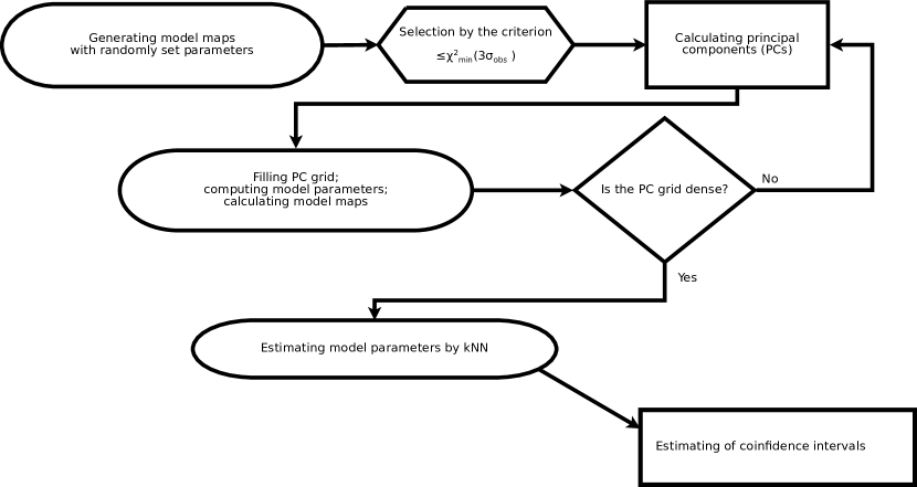
5mm normal

Figure 1: Parameter determination diagram for fitting model spectral maps into observed ones.

In the course of preliminary analysis, we determined the coordinates of the map’s central point (the center of the core) and the source velocity from the observational data in the optically thin line. Using a random number generator, we then created a set of model parameters with sufficiently wide ranges and calculated the model spectral maps and values of the error function. Within this set, we selected those parameters that satisfy the inequality $\chi^{2}\leq\chi_{min}^{2}(3\sigma_{obs})$, where $\chi_{min}^{2}(3\sigma_{obs})$ is the value of the error function at those model parameters that yield the minimum value $\chi^{2}$ for a given set when noise with a standard deviation of $3\sigma_{obs}$ is added to the observed intensities. For the resulting parameter sample, we calculated matrices of the direct and inverse transformation into the PC-space, reduced the number of components, and filled the remaining space with a regular grid. The grid nodes were transformed using the inverse transformation into the values of the physical parameters.

Choosing a sufficient number of PCs is not a simple problem since any dimensionality reduction method causes information loss. An overview of possible options for solving this problem is given in Appendix to [42] and in the references to that paper. In linear PCA, which we applied, the loss of information can manifest itself in biased values of the physical parameters after the direct and inverse transformations. The number of remaining PCs, which determines the extent of the loss, was chosen in such a way that the ratio of the eigenvector sum for the PC covariance matrix to the eigenvector sum for the covariance matrix of the physical parameters differed from unity (the value in the case of the identity transformation) by no more than 10% and the bias in the parameter estimates did not create systematic errors [42, 43].

The final step was to calculate the physical parameter values corresponding to the exact minimum of the error function and estimate the errors. To this end, we used the $k$NN method [33], which we previously applied to estimate the physical parameters of the dense core of S255N [44]. The $k$NN method is similar to the least-squares method, but unlike the latter, it does not adjust the model parameters to the observed spectra but calculates the optimal parameter values from the previously obtained spectra by the same criterion. This method enables regression analysis between a set of model maps with different parameters and the observed map. Thus, among all the model maps, we found $k$ nearest ones to the observed map by the criterion of the minimum of the mean $\chi^{2}$ value. When there was no such minimum ($\chi^{2}$ increases with increasing $k$, and averaging across the models increases the error function), a denser grid was needed for PCs in the region near the supposed minimum. The optimal value of the $p$ parameter was the $\chi^{2}$-weighed mean over $k$ selected instances:

$$p=\frac{\sum_{i=1}^{\rm k}p_{i}/\chi_{i}^{2}}{\sum_{i=1}^{\rm k}1/\chi_{i}^{2}}\hskip 5.69054pt,$$ (2)

where $p_{i}$ and $\chi_{i}^{2}$ are the values of the parameter and error function for the $i$th point in the parameter space, respectively.

Using maps of the object in several spectral lines of different optical depths, we can narrow down the range of confidence values by fitting the model spectra into these maps simultaneously. In this case, additional model parameters are the relative abundances of the molecules. The total error for the maps in several lines ($n_{lines}$) is written as

$$\chi^{2}=\frac{1}{N_{p}-n}\sum_{k=1}^{n_{lines}}\sum_{j=1}^{N_{k}}\sum_{i=1}^{m_{k}}\frac{(I_{ijk}^{obs}-I_{ijk}^{mod})^{2}}{\sigma_{jk}^{2}}\hskip 5.69054pt,$$ (3)

where $N_{p}=\sum_{k=1}^{n_{lines}}N_{k}\times m_{k}$; $N_{k}$ is the number of spatial points in the map in the $k$th line; $m_{k}$ is the number of channels in the spectrum of the $k$th line; and $\sigma_{jk}$ is the standard deviation of the observed spectrum in the $k$th line at point $j$.

Since the parameter space is curvilinear, the confidence regions for the probable parameter values were determined by applying a cross-section of the multidimensional error function by the hyperplane $\chi^{2}=\chi^{2}_{\sigma}$. The calculation of $\chi^{2}_{\sigma}$ does not depend on the choice of the basis; it is convenient to perform it in the PC space. The threshold value was $\chi^{2}_{\sigma}=\chi_{min}^{2}(pc_{l}^{opt}\pm\sigma_{pc_{l}})$, i.e., the value of the error function in the case where one of the PCs ($pc_{l}$) takes a value displaced from the optimal one by $\sigma_{pc_{l}}$ and the other components vary in such a way that the error function takes the minimum value. As $\sigma_{pc_{l}}$, we took a symmetric estimate for the error of $pc_{l}$, which is a diagonal element of the matrix inverse to the Hesse matrix, (see, e.g., [45–47]), which element was calculated as

$$\beta_{lm}=\sum_{k=1}^{n_{lines}}\sum_{j=1}^{N_{k}}\sum_{i=1}^{m_{k}}\frac{1}{\sigma_{jk}^{2}}\frac{\partial I_{ijk}^{mod}}{\partial pc_{l}}\frac{\partial I_{ijk}^{mod}}{\partial pc_{m}}\hskip 5.69054pt,$$ (4)

where $pc_{l},pc_{m}$ are different PCs. The derivatives were calculated numerically over the entire set of model maps. After estimating the threshold value of $\chi^{2}_{\sigma}$, we constructed two-dimensional projections of the error function and its hyperplane cross-section in the plane of different pairs of model parameters and determined the confidence regions. In the general case, these regions are not symmetrical relative to the optimal parameter values. An example of using two-dimensional projections of the error function for estimating the confidence ranges of model parameters in the analysis of the L1287 molecular line maps is presented in Section 3.2.

3 ESTIMATING THE PHYSICAL PARAMETERS OF THE L1287 CORE

3.1 Observational Manifestations of L1287

The dark cloud L1287 is located at a distance of $0.93\pm 0.03$ kpc [48] and is shaped as a filament of $\sim 10$ pc in length. A dust emission map in continuum at a wavelength of 500 $\mu$m, which was acquired using the Herschel telescope towards L1287 (observation ID: 1342249229 [49]), is shown in Fig. 2 (different shades). In the central part of the cloud, there is a high-density core, which contains the source IRAS 00338+6312 [34]. In the core, two objects of type FU Ori (RNO 1B/1C) were also detected [51–53], as well as a cluster of IR and radio sources, likely associated with young stellar objects of low and intermediate mass [54, 53]. Maser lines of water [55] and methanol molecules [56] were also detected there. Molecular line observations [34, 57, 58] revealed a bipolar outflow in the northeastern and southwestern directions. Based on observations in the H¹³CO⁺(1–0) line, it was concluded [59] that the central part of the core contains a rotating disk of radius $\sim 7800$ AU, with the bipolar outflow oriented along the disk axis. Based on interferometry observations, the inner part of the core ($\mathrel{\mathchoice{\vbox{\offinterlineskip\halign{\hfil$\displaystyle#$\hfil\cr<\cr\sim\cr}}}{\vbox{\offinterlineskip\halign{\hfil$\textstyle#$\hfil\cr<\cr\sim\cr}}}{\vbox{\offinterlineskip\halign{\hfil$\scriptstyle#$\hfil\cr<\cr\sim\cr}}}{\vbox{\offinterlineskip\halign{\hfil$\scriptscriptstyle#$\hfil\cr<\cr\sim\cr}}}}0.1$ pc) is highly fragmented [60, 61]. In [61], a kinematic model was proposed for the central part of the L1287 core. In this model, gas motions towards the center from the core’s outer regions become nonisotropic near the center and transform into the disk rotation.

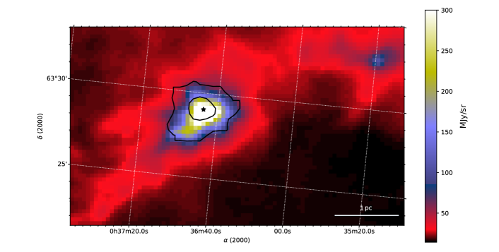
5mm normal

Figure 2: Map of the L1287 dark cloud at wavelength 500 $\mu$m from the Herschel telescope observational data. The integrated intensity isolines in the HCO⁺(1–0) line correspond to 20% and 50% of the maximum (38.6 K km/s) [50]. The star symbol indicates the source IRAS 00338+6312.

The emission region sizes of the L1287 core in the different molecular lines and in continuum vary from a few tenths to one parsec [34, 62–65]; the shape of the emission regions is roughly close to a spherically symmetric one. The profiles of optically thick lines in the L1287 core are asymmetric and have two peaks separated by a dip, with the amplitude of the blue peak in most of the maps being higher than that of the red one [25, 34, 62].

We observed the L1287 core in 2015 with the OSO-20m telescope in different lines in the frequency range of $\sim 85-89$ GHz [50]. The angular resolution of the observations was $\sim 42^{\prime\prime}$, which corresponds to a linear resolution of $\sim 0.19$ pc. The integrated intensity isolines of the HCO⁺(1–0) line, which were superimposed onto the Herschel map, are shown in Fig. 2. The asymmetric profiles of HCO⁺(1–0) and HCN(1–0), observed virtually throughout the entire region ($\sim 0.9$ pc), and the symmetric profiles of optically thin lines, which intensity peaks are close to the dips in the profiles of optically thick lines, are likely to be indicative of gas contraction.

3.2 Map Analysis of the L1287 Core in Different Molecular Lines

The algorithm presented in Section 2 was applied for estimating the physical parameters of the L1287 core. To this end, we performed the fitting of the maps in the lines of HCO⁺(1–0), H¹³CO⁺(1–0), HCN(1–0), and H¹³CN(1–0), calculated within the 1D microturbulent model (see Appendix), into the central part of the observed region with an angular size of 80^′′ ($\sim 0.4$ pc). The physical parameters (density, turbulent and systematic velocities, and kinetic temperature) were dependent on the distance to the center, $r$, by the law $P=P_{0}/(1+(r/R_{0})^{\alpha_{p}}$), where $R_{0}$ is the radius of the central layer. The free model parameters were the values $P_{0}$ for the radial profiles of density and turbulent and systematic velocities ($n_{0}$, $V_{turb}$, $V_{sys}$, respectively); the power-law indices $\alpha_{p}$ ($\alpha_{n}$, $\alpha_{turb}$, $\alpha_{sys}$), the relative abundances of the molecules ($X$), independent of the radial distance; and the outer radius ($R_{max}$) of the core.

The kinetic temperature profile was set at $T=80$ K$/(1+(r/R_{0})^{0.3})$ and kept unchanged during the calculations. Meanwhile, the kinetic temperature varied from 40 K in the central layer to $\mathrel{\mathchoice{\vbox{\offinterlineskip\halign{\hfil$\displaystyle#$\hfil\cr<\cr\sim\cr}}}{\vbox{\offinterlineskip\halign{\hfil$\textstyle#$\hfil\cr<\cr\sim\cr}}}{\vbox{\offinterlineskip\halign{\hfil$\scriptstyle#$\hfil\cr<\cr\sim\cr}}}{\vbox{\offinterlineskip\halign{\hfil$\scriptscriptstyle#$\hfil\cr<\cr\sim\cr}}}}20$ K on the periphery, which is generally consistent with estimates based on observational data (see, e.g., [62, 63, 65, 50]). Although the dust temperatures for L1287 from the Herschel data are $\sim 15-24$ K (http://www.astro.cardiff.ac.uk/research/ViaLactea/) [66], the data of interferometric observations suggest that in the inner regions of the L1287 core ($\mathrel{\mathchoice{\vbox{\offinterlineskip\halign{\hfil$\displaystyle#$\hfil\cr<\cr\sim\cr}}}{\vbox{\offinterlineskip\halign{\hfil$\textstyle#$\hfil\cr<\cr\sim\cr}}}{\vbox{\offinterlineskip\halign{\hfil$\scriptstyle#$\hfil\cr<\cr\sim\cr}}}{\vbox{\offinterlineskip\halign{\hfil$\scriptscriptstyle#$\hfil\cr<\cr\sim\cr}}}}0.1$ pc), where the fragmentation effects are strong, the kinetic temperature of fragments may be as high as $\sim 80-100$ K (see [60]). Thus, in the calculations, 40 K was taken as an average value of kinetic temperature in the central layer, the radius of which ($R_{0}$) was set at $2\times 10^{16}$ cm ($\sim 1300$ AU).

The radial velocity and the core center coordinates were estimated from the H¹³CO⁺(1–0) line. Then, we used a map in the HCO⁺(1–0) line to search for the minimum of the error function. Using a random number generator, we formed an array of 6000 parameter values, which were randomly and equiprobably distributed in the following ranges of eight parameters: $n_{0}$=[$10^{6.5}...10^{9}$] cm^-3, $\alpha_{n}$=[1.3…2.5], $V_{turb}$=[1.4…7.5] km/s, $\alpha_{turb}$=[0.1…0.7], $V_{sys}$=[–1.3…–0.2] km/s, $\alpha_{sys}$=[–0.2…0.4], $X$(HCO⁺)=[$10^{-10.5}...10^{-8}$], $R_{max}$=[$10^{17.7}-10^{19.2}$] cm. Although we assumed that these ranges were certain to include the optimal parameter values for the L1287 core, their boundaries were not rigid and could be expanded by means of the inverse transformation from the PC space.

For each value in the parameter array, we calculated a map in the HCO⁺(1–0) line and the error function. Based on the accepted criterion, $\chi^{2}\leq\chi_{min}^{2}(3\sigma_{obs})$, we selected 246 values from the initial set. This number was enough to construct the statistics in the PC space. For these values, we calculated a set of PCs using a procedure from the $scikit$-$learn$ library [67]. Using the dependence of $R$, the ratio of the sum of the diagonal components in the PC covariance matrix to the sum of the diagonal components in the covariance matrix of the physical parameters, on the number of components, we estimated the minimum number of PCs required to represent the physical parameters (Fig. 3). Figure 3 shows that the five PCs represent to a sufficient extent the eight physical parameters at a level of $R=0.9$. For the five PCs, the difference after the inverse transformation did not exceed 5% of the grid step for all the parameters, suggesting no distortions in subsequent calculations and no error accumulation. Figure 3 also shows the contribution of each component to the relative covariance matrix of the PCs.

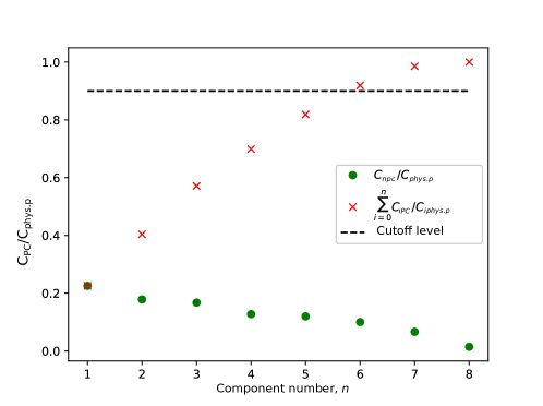
5mm normal

Figure 3: Dependence of the ratio of the sum of the diagonal components in the PC covariance matrix and the sum of the diagonal components in the covariance matrix of the physical parameters on the number of components (red crosses). The green circles show the contribution of an individual component to the relative PC covariance matrix. The dashed horizontal line indicates a cutoff level of 0.9.

In the space of the five remaining PCs, we constructed a uniform five-dimensional grid with a center at the point of minimum of the error function; the grid size was consistent with $6\Delta(pc_{i})$, where $\Delta(pc_{i})$ is a standard deviation of the $i$th PC values, which was calculated from the selected set of points. The PC array was recalculated to the array of the physical parameter values, for which we calculated the spectral maps and estimated the error functions. From the calculated model maps, we estimated the optimal physical parameters from the HCO⁺(1–0) data by the $k$NN method. Varying by the least squares method, the relative abundances of H¹³CO⁺, HCN, and H¹³CN, we fitted the corresponding model spectral maps into the observed ones. In so doing, we also slightly adjusted the parameters within the error ranges calculated from the HCO⁺(1–0) data. By comparing the set of model spectral maps with the observed ones, we estimated the global error function in the four lines by equation (3). The resulting model spectra proved to be close to the observed ones up to a scale of $\sim 0.8$ pc, which confirmed the relevance of the applied model.

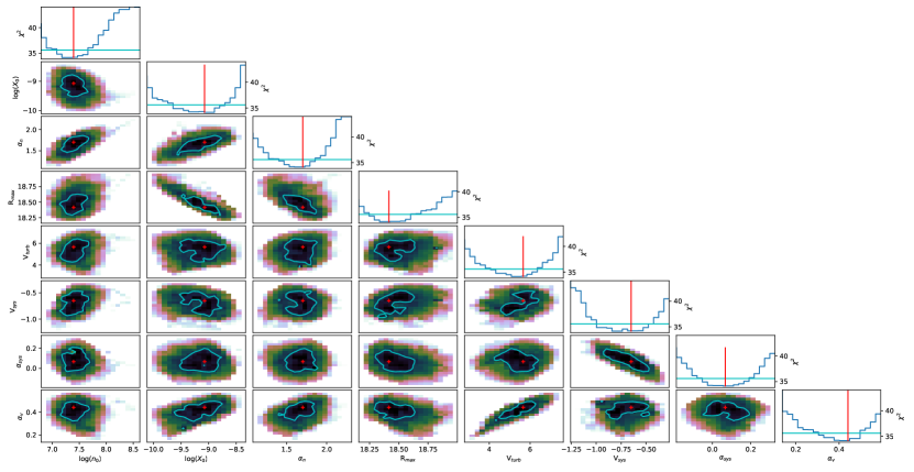
5mm normal

Figure 4: Projections of the eight-dimensional error function $\chi^{2}$ onto the planes of the different parameter pairs calculated from the fitting of the model spectral maps in the lines HCO⁺(1–0), H¹³CO⁺(1–0), HCN(1–0) and H¹³CN(1–0) into the observed maps in the L1287 core. The dependencies of the error function on the individual parameters are given over each projection column. The red dots in the diagrams and the red vertical lines in the upper plots indicate the global minimum of the error function, which was obtained by $k$NN. The confidence regions for the optimal parameter values, which were calculated from the hyperplane $\chi_{\sigma}^{2}$ cross-sections of the error function, are shown with blue contours and horizontal lines in the two-dimensional projections and one-dimensional plots, respectively.

Figure 4 presents a set of projections of the eight-dimensional error function onto the planes of the different parameter pairs and the error function projection dependencies on each of the parameters. It follows from the two-dimensional projections and the dependencies, that the model has a global minimum, and a confidence level can be determined for each of the parameters. Correlations are observed between some of the parameters. A clear correlation is observed between $R_{max}$ and the relative abundance of HCO⁺ ($X_{0}$), between $\alpha_{n}$ and $X_{0}$, and between the turbulent and systematic velocities in the central layer and the corresponding power-law indices of the radial profiles of these parameters. A weaker correlation exists between $\alpha_{n}$ and $n_{0}$ and between $R_{max}$ and $\alpha_{n}$. The exact position of the minimum was estimated by the $k$NN method from all the lines; it is marked by a red cross in the two-dimensional projections and by red vertical lines in the $\chi^{2}$ projection dependencies on individual parameters. The confidence regions were calculated using a cross-section of the error function by the hyperplane $\chi_{\sigma}$. The projections of the error function cross-sections by the $\chi_{\sigma}$ hyperplane are in fact contours in the planes of parameter pairs; they correspond to horizontal lines on upper plots (see Fig. 4). The confidence regions are not symmetric with respect to the optimal values. The distortions in the shape of the contours are due to observational noise and the discrete filling of the parameter space. When analyzing the dependencies of $\chi^{2}$ on individual parameters in broader ranges than those shown in Fig. 4, we found additional local minima, which values are, however, greater than the one corresponding to the global minimum and the corresponding parameter values considerably deviate from independent estimates.

The estimates for the physical parameters of the L1287 core, which correspond to the global minimum of the error function, and the uncertainties of these estimates, which correspond to the boundaries of the confidence regions (Fig. 4), are given in Table 1. It should be noted that in accordance with the specified form of the radial profiles, the physical parameter values in the central layer are twice as low as the corresponding values of $n_{0}$, $V_{turb}$, and $V_{sys}$.

0mm

Table 1: Resulting values of the physical parameters

Parameter	Value
$n_{0}$(cm-3), 107	2.6${}_{-1.3}^{+1.7}$
$\alpha_{n}$	1.7${}_{-0.3}^{+0.1}$
Vturb (km/s)	5.6${}_{-1.4}^{+0.7}$
$\alpha_{turb}$	0.44${}_{-0.13}^{0.05}$
Vsys (km/s)	–0.66${}_{-0.24}^{+0.21}$
$\alpha_{sys}$	0.1${}_{-0.13}^{+0.08}$
Rmax(pc)	0.8${}_{-0.25}^{+0.2}$
X(HCO+), 10-9	1.0${}_{-0.4}^{+0.5}$
X(H13CO+), 10-11	3.7${}_{-2.0}^{+2.4}$
X(HCN), 10-9	2.5${}_{-1.1}^{+1.4}$
X(H13CN), 10-11	8.5${}_{-4.8}^{+5.3}$

4 RESULTS AND DISCUSSION

Figures 5 and 6 show the spectral maps for the central part of the L1287 core ($\sim 0.4$ pc) in the HCO⁺(1–0), HCN(1–0), H¹³CO⁺(1–0), and H¹³CN(1–0) lines with the fitted model spectra corresponding to the global minimum of the error function. The asymmetry and dip in the observed profiles of the optically thick lines of HCO⁺(1–0) and HCN(1–0) are well reproduced by the model. In the central and southwestern parts of the analyzed region, the spectra of the optically thick lines exhibit high-velocity gas emission, which was ignored in the model calculations. The slight discrepancy between the model and observed spectra at the edges of the observed region may be due to a difference from spherical symmetry. The diameter (1.6 pc) of the model cloud exceeds the observed sizes of the emission regions in the different molecular lines, the dense gas indicators, HCO⁺(1–0), HCN(1–0), and NH₃(1,1) ($\sim 0.3-0.5$ pc) [62, 63, 50], since it comprises the low-density outer layers, which cause the dip in the profiles of the optically thick lines as they absorb the emission from the central layers.

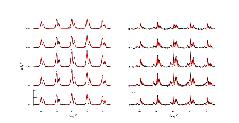
5mm normal

Figure 5: Results of fitting the model spectra of HCO⁺(1–0) (left) and HCN(1–0) (right) (smooth red curves) into the observed ones (histograms, black lines) in the central part of the L1287 core. The horizontal axis plots the velocities in the range from –33 to –5 km/s.

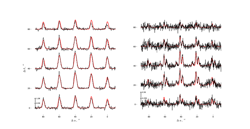
5mm normal

Figure 6: Results of fitting the model spectra of H¹³CO⁺(1–0) (left) and H¹³CN(1–0) (right) (smooth red curves) into the observed ones (histograms, black lines) in the central part of the L1287 core. The horizontal axis plots the velocities in the range from –28.5 to –7 km/s.

The calculated physical parameters of the core are consistent, considering the errors (see Table 1), with estimates obtained from the data of independent observations. Thus, the model column density of molecular hydrogen for a region of radius $\sim 20^{\prime\prime}$ agrees with the value calculated from the data of dust observations with the Herschel telescope [66] ($4.6_{-2.3}^{+3.0}$ $10^{23}$ cm^-2 and $(1.8\pm 1.2)\,10^{23}$ cm^-2, respectively). The core mass calculated from the model for a region of radius $\sim 0.6$ pc is $\sim 1200$ M₀; considering the error ($\mathrel{\mathchoice{\vbox{\offinterlineskip\halign{\hfil$\displaystyle#$\hfil\cr>\cr\sim\cr}}}{\vbox{\offinterlineskip\halign{\hfil$\textstyle#$\hfil\cr>\cr\sim\cr}}}{\vbox{\offinterlineskip\halign{\hfil$\scriptstyle#$\hfil\cr>\cr\sim\cr}}}{\vbox{\offinterlineskip\halign{\hfil$\scriptscriptstyle#$\hfil\cr>\cr\sim\cr}}}}50$%), associated primarily with the error of $n_{0}$, this mass is consistent with the value of 810 M₀, obtained from the observations of dust for a region of similar radius [65]. Neither does the power-law index of the radial density profile $1.7_{-0.3}^{+0.1}$ contradict the value of $1.25\pm 0.2$, obtained from the observations of dust in continuum [65]. Both of these estimates lie in the value range for the power-law index of the density profile obtained for samples of dense cores associated with regions of massive star and star cluster formation (see, e.g., [65, 68, 69]) but are lower than 2, the value predicted by the isothermal sphere [8] and global collapse models [13].

The model abundance ratios of the main and rarer isotopes ([HCO⁺]/[H¹³CO⁺] and [HCN]/[H¹³CN]) are lower by a factor of $\sim 2$ than the isotope ratio [¹²C]/[¹³C]$\sim 58$, calculated from the heliocentric dependence of this ratio [70] for $R_{G}\sim 9$ kpc (L1287). However, the uncertainties of the model abundance ratios are rather high ($\mathrel{\mathchoice{\vbox{\offinterlineskip\halign{\hfil$\displaystyle#$\hfil\cr>\cr\sim\cr}}}{\vbox{\offinterlineskip\halign{\hfil$\textstyle#$\hfil\cr>\cr\sim\cr}}}{\vbox{\offinterlineskip\halign{\hfil$\scriptstyle#$\hfil\cr>\cr\sim\cr}}}{\vbox{\offinterlineskip\halign{\hfil$\scriptscriptstyle#$\hfil\cr>\cr\sim\cr}}}}80$%) to make further conclusions from this discrepancy. To verify the results obtained, they should be compared with the chemical modeling results.

The turbulent velocity falls rather sharply with the distance from the center (from 2.8 km/s in the central layer to $\sim 0.6$ km/s in the outer layer), which is necessary for reproducing the shape of the dip in the HCO⁺(1–0) and HCN(1–0) spectra (solid curve $1$ in Fig. 7, right panel). The contraction velocity decreases weakly in absolute terms with the distance from the center ($\sim 0.33$ km/s in the central layer and $\sim 0.25$ km/s in the outer layer) (dashed curve $1$ in Fig. 7, right panel). Its average value across the model cloud is $0.26\pm 0.09$ km/s, which does not contradict the value of $\sim 0.22$ km/s, calculated from the HCO⁺(1–0) line parameters for the point (60^′′,40^′′) by the formula of the two-layer model [20] (the value given in [50] is underestimated).

5mm

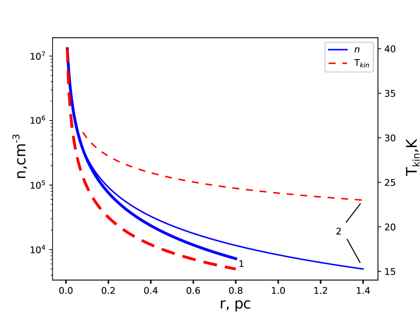
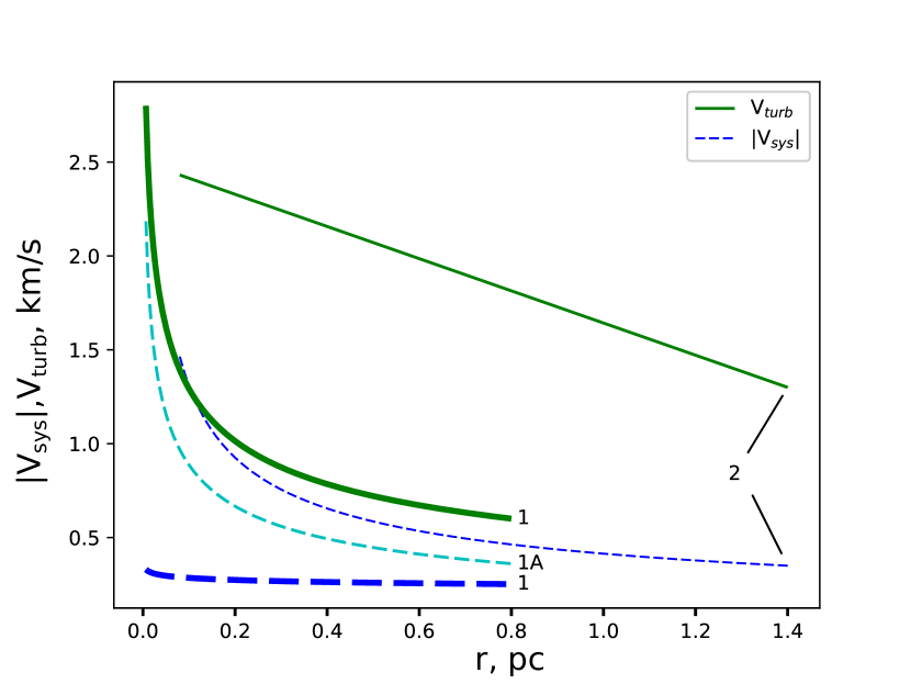
normal

Figure 7: Model radial profiles of density and kinetic temperature (left panel) and contraction and turbulent velocities (right panel). Profiles were obtained in this work ($1$) and those from [25] ($2$). The cloud radius in the latter model was set to 1.4 pc, consistent with a distance of 0.93 kpc to L1287. The $1A$ mark in the right panel shows the contraction velocity profile obtained in our model with a fixed value of the power index, 0.5.

The power-law index of the radial profile for contraction velocity obtained in the model calculations considering errors proved to be lower than 0.5 for the case of gas collapse onto the protostar in free fall [8, 10, 13]. In [25], the observational data for the core 0038 + 6312 (L1287) in the HCO⁺(1–0), CS(2–1), and CS(5–4) lines were compared with the calculated results for the model with the density and contraction velocity profiles $\propto r^{-3/2}$ and $\propto r^{-1/2}$, respectively. Although the intensities and widths of the model spectra proved to match the observed ones in the direction of individual positions quite well, considering the sensitivity and spectral resolution of the data, the dip in the HCO⁺(1–0) line profiles was not reproduced (see [25]). This is due to the difference of the radial profiles for velocity, which were assumed in the model [25], from the profiles obtained in our calculations (Fig. 7, right panel). The left panel in Fig. 7 shows the radial profiles of density and kinetic temperature for our model and for the model [25].

As shown in the model of the global hierarchical collapse (see, e.g., [13, 16]), if the core is globally out-of-equilibrium, it experiences contraction with a constant velocity and this contraction continues in the outer layers even after the protostar formation. For comparison, we fitted the model maps into the observed ones for the case where the power-law index of the radial profile of systematic velocity was fixed at 0.5. The corresponding velocity profile is marked $1A$ in Fig. 7 (right panel). Figure 8 shows the observed HCO⁺(1–0) and HCN(1–0) lines for the point (60^′′,40^′′) near the core center and the model spectra for the power-law index of systematic velocity of 0.1, which corresponds to the global minimum of the error function, and for the case when the index is 0.5, respectively. Upon comparison of the spectra, the model with the index 0.1 more accurately reproduces the intensities and widths of the asymmetric HCO⁺(1–0) profiles and, specifically, the profiles of three hyperfine HCN(1–0) components than the model with the index 0.5. A similar conclusion is true for the other points. Although in the southwestern part, the high-velocity emission associated with bipolar outflow more strongly distorts the spectra shape (Fig. 5), which makes it more difficult to compare the models. The fact that the value obtained in the model with the power-law index of the velocity profile as a free parameter turned out to be lower than 0.5 may suggest a likelihood of nonuniform gas contraction in the core – with constant velocity in the extended envelope and with the $\propto r^{-1/2}$ profile in the region near the center. The use of the model with a single power-law index gives a weighted average for the entire core in this case.

5mm

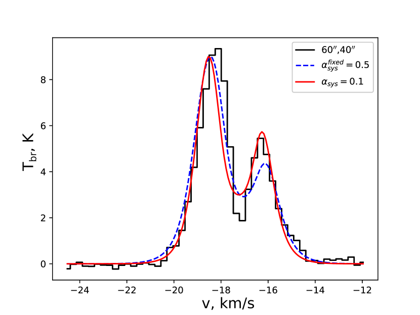
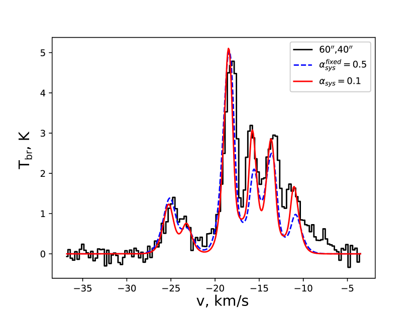
normal

Figure 8: Observed and model profiles of the lines HCO⁺(1–0) (left) and HCN(1–0) (right) towards the (60^′′,40^′′) position for models with different values of the power-law index in the radial profile of contraction velocity.

Although we used a rather simplified 1D model with uniform power-law indices for the radial profiles of the physical parameters, it allows using the developed algorithm for fitting the model spectral maps into the observed ones with PCA and $k$NN to reproduce accurately the observed HCO⁺(1–0), HCN(1–0), H¹³CO⁺(1–0), and H¹³CN(1–0) line maps and estimate the radial profiles of the parameters in outer regions of the L1287 core ($r\mathrel{\mathchoice{\vbox{\offinterlineskip\halign{\hfil$\displaystyle#$\hfil\cr>\cr\sim\cr}}}{\vbox{\offinterlineskip\halign{\hfil$\textstyle#$\hfil\cr>\cr\sim\cr}}}{\vbox{\offinterlineskip\halign{\hfil$\scriptstyle#$\hfil\cr>\cr\sim\cr}}}{\vbox{\offinterlineskip\halign{\hfil$\scriptscriptstyle#$\hfil\cr>\cr\sim\cr}}}}0.1$ pc). Some of the differences between the model and observed spectra can be eliminated, apparently, within more complex models with composite radial profiles of the parameters and also within 2D or 3D models considering the possible spatial inhomogeneity of the velocity field, rotation, and high-velocity outflows. To reduce errors in the calculated parameters and to confirm the conclusion about the possible global contraction of the L1287 core, further observations are required in molecular lines of different optical depths with better spatial and spectral resolution.

A distinctive feature of the developed algorithm is its lack of ties to a specific model and its capability of simultaneous analysis of spectral maps with different spatial resolutions and sizes, as well as maps in continuum. The main constraint is only the computational time required to construct the necessary statistics.

5 CONCLUSIONS

The results of this work can be summarized as follows:

(1) An algorithm was developed for finding the global minimum of the multidimensional error function and calculating the optimal parameter values when fitting model spectral maps into observed ones. The algorithm is based on applying principal component analysis to a given range of parameters, as a result of which a reduction is achieved in the model’s dimensionality and in the coupling degree between the parameters. Thus, the region of the minimum is determined. The optimal parameter values are calculated using the $k$ nearest neighbors method. Confidence regions for the optimal parameter values are determined using a cross-section of the error function by a hyperplane calculated in the PC space and its projections onto the various pairs of the parameters. The algorithm is not tied to a specific model.

(2) The algorithm was used to perform the fitting of the model maps in the HCO⁺(1–0), H¹³CO⁺(1–0), HCN(1–0), and H¹³CN(1–0) lines into the observed maps of the protostellar core of L1287, in which the formation of a young stellar cluster is underway, and the asymmetry of the profiles of optically thick lines indicates contraction. The maps were calculated within a spherically symmetric 1D model in which the physical parameters (density and turbulent and systematic velocities) were functions of the distance from the center. Optimal values were calculated for the model parameters, and their errors were determined. It was found that density in the L1287 core decreases with the distance from the center as $\propto r^{-1.7}$ while turbulent and contraction velocities decrease as $\propto r^{-0.4}$ and $\propto r^{-0.1}$, respectively. The absolute value of the power-law index for the radial profile of contraction velocity, considering the probable error, is less than 0.5, a value expected in the case of gas collapse onto the protostar in free fall. This result may indicate global contraction in the L1287 core, which was predicted in several theoretical works.

APPENDIX. MODEL DESCRIPTION

Excitation of rotational levels of the HCO⁺ and HCN molecules and their isotopes and the profiles of the (1–0) transitions were calculated within a spherically symmetric microturbulent model. The model cloud is a set of concentric layers in which a certain physical parameter (density, kinetic temperature, turbulent and systematic velocity) was set constant, changing from one layer to another by the relationship $P=P_{0}/(1+(r/R_{0})^{\alpha_{p}}$), where $r$ is the distance from the center and $R_{0}$ is the radius of the central layer. This functional dependence, which is a simplified form of the Plummer function, is used quite often as a model density profile (see, e.g., [22]) to avoid singularity at the center. In our model, this form of the dependence was used for all the parameters. The values of $P_{0}$ and $\alpha_{p}$ for each parameter were varied while fitting the model profiles into the observed ones. The kinetic temperature profile was taken as $T=80$ K$/(1+(r/R_{0})^{0.3})$ and remained unchanged during calculations. It should be noted that kinetic temperature affects the intensities of the calculated HCO⁺(1–0) and HCN(1–0) lines to a lesser degree than density and concentration. Turbulent velocity was a parameter that gives an additional contribution - aside from the thermal one - to the local width of the lines. The relative molecular abundance was independent of radial distance. When calculating the excitation of HCN and H¹³CN, the hyperfine structure of the rotational spectrum and the overlapping of closely located hyperfine components [40, 71] was taken into account. The description of the model and calculation techniques for radiation transfer in the case of HCN is given in the Appendix to [40]. In our version of this model, the layer width increases by the power law with the distance from the center, and the radial profile of systematic velocity, which gives a Doppler shift to the local profile of the line, is taken into account. The calculations were conducted for 14 layers. The calculations used collisional probabilities of HCO⁺–H₂ [72] and HCN–H₂ taking into account hyperfine structure [73].

Excitation of rotational levels of a certain molecule was calculated by an iterative method, sequentially for one point in each layer, the radial distance of which is equal to the geometric mean of the inner and outer radii of the layer. To this end, a system of population balance equations was solved, while the populations in other layers were considered unchanged. After reaching the outer layer, the populations in each layer were compared with the values obtained in the previous iteration, and the process was repeated [40]. To increase the accuracy of calculating the radiation transfer in a moving medium, each layer was additionally divided into ten sublayers, with different systematic velocities. A test comparison of the calculated results for this model with the calculated results in [74] for a molecule with two energy levels showed that the calculated populations differ by no more than 0.4% in the case of line optical depth of $\mathrel{\mathchoice{\vbox{\offinterlineskip\halign{\hfil$\displaystyle#$\hfil\cr<\cr\sim\cr}}}{\vbox{\offinterlineskip\halign{\hfil$\textstyle#$\hfil\cr<\cr\sim\cr}}}{\vbox{\offinterlineskip\halign{\hfil$\scriptstyle#$\hfil\cr<\cr\sim\cr}}}{\vbox{\offinterlineskip\halign{\hfil$\scriptscriptstyle#$\hfil\cr<\cr\sim\cr}}}}60$.

The model code, written in Fortran, was controlled by means of a module written in Python. Model spectra were calculated for the different impact parameters. Using the astropy.convolve_fft procedure [75], the resulting maps were convoluted channel by channel with a two-dimensional Gaussian of width 40^′′ (the width of the main beam of the OSO-20m radio telescope at a frequency of $\sim 90$ GHz). The model spectra were fitted into the observed ones using a PCA- and $k$NN-based algorithm (Section 2), written in Python.

REFERENCES

1. J. C. Tan, M. Beltrán, P. Caselli, F. Fontani, A. Fuente, M. R. Krunholz, C. F. McKee, and A. Stolte, in $Protostars\leavevmode\nobreak\ and\leavevmode\nobreak\ Planets\leavevmode\nobreak\ VI$, Ed. by H. Beuther, R. S. Klessen, C. P. Dullemond, and Th. Henning (Univ. of Arizona Press, Tucson, 2014), p. 149.

2. F. Motte, S. Bontemps, and F. Louvet, Ann. Rev. Astron. Astrophys. 56, 41 (2018).

3. Ph. André, A. Men’shchikov, S. Bontemps, V. Könyves, et al., Astron. Astrophys. 518, L102 (2010).

4. Ph. André, J. Di Francesco, D. Ward-Thompson, S.-I. Inutsuka, R. E. Pudritz, and J. E. Pineda, in $Protostars\leavevmode\nobreak\ and\leavevmode\nobreak\ Planets\leavevmode\nobreak\ VI$, Ed. by H. Beuther, R. S. Klessen, C. P. Dullemond, and Th. Henning (Univ. of Arizona Press, Tucson, 2014), p. 27.

5. F. Nakamura, K. Sugitani, T. Tanaka, H. Nishitani, et al., Astrophys. J. Lett. 791, L23 (2014).

6. Y. Contreras, G. Garay, J. M. Rathborne, and P. Sanhueza, Mon. Not. R. Astron. Soc. 456, 2041 (2016).

7. L. K. Dewangan, L. E. Pirogov, O. L. Ryabukhina, D. K. Ojha, and I. Zinchenko, Astrophys. J. 877, 1 (2019).

8. F. H. Shu, Astrophys. J. 214, 488 (1977).

9. F. H. Shu, F. C. Adams, and S. Lizano, Ann. Rev. Astron. Astrophys. 25, 23 (1987).

10. C. F. McKee and J. C. Tan, Astrophys. J. 585, 850 (2003).

11. Y. Zhang and J. C. Tan, Astrophys. J. 853, 18 (2018).

12. D. E. McLaughlin and R. E. Pudritz, Astrophys. J. 476, 750 (1997).

13. E. Vázquez-Semadeni, A. Palau, J. Ballesteros-Paredes, G. C. Gómez, and M. Zamora-Avilés, Mon. Not. R. Astron. Soc. 490, 3061 (2019).

14. R. B. Larson, Mon. Not. R. Astron. Soc. 145, 271 (1969).

15. M. V. Penston, Mon. Not. R. Astron. Soc. 144, 425 (1969).

16. R. Naranjo-Romero, E. Vázquez-Semadeni, and R. M. Loughnane, Astrophys. J. 814, 48 (2015).

17. D. Mardones, P. C. Myers, M. Tafalla, D. J. Wilner, R. Bachiller, and G. Garay, Astrophys. J. 489, 719 (1997).

18. N. J. Evans II, Ann. Rev. Astron. Astrophys. 37, 311 (1999).

19. Ya. Pavlyuchenkov, D. Wiebe, B. Shustov, Th. Henning, R. Launhardt, and D. Semenov, Astrophys. J. 689, 335 (2008).

20. P. C. Myers, D. Mardones, M. Tafalla, J. P. Williams, and D. J. Wilner, Astrophys. J. 465, L133 (1996).

21. C. W. Lee, P. C. Myers, and M. Tafalla, Astrophys. J. Suppl. 136, 703 (2001).

22. C. H. De Vries and P. C. Myers, Astrophys. J. 620, 800 (2005).

23. J. L. Campbell, R. K. Friesen, P. G. Martin, P. Caselli, J. Kauffmann, and J. E. Pineda, Astrophys. J. 819, 143 (2016).

24. S. Zhou, N. J. Evans, II, C. Kömpe, and C. M. Wamsley, Astrophys. J. 404, 232 (1993).

25. R. N. F. Walker and M. R. W. Masheder, Mon. Not. R. Astron. Soc. 285, 862 (1997).

26. G. Narayanan, G. Moriarty-Schieven, C. K. Walker, and H. M. Butner, Astrophys. J. 565, 319 (2002).

27. Ya. N. Pavlyuchenkov and B. M. Shustov, Astron. Rep. 48, 315 (2004).

28. L. Pagani, I. Ristorcelli, N. Boudet, M. Giard, A. Abergel, and J.-P. Bernard, Astron. Astrophys. 512, A3 (2010).

29. G. Garay, D. Mardones, Y. Contreras, J. E. Pineda, E. Servajean, and A. E. Guzmán, Astrophys. J. 799, 75 (2015).

30. K. R. Opara and J. Arabas, Swarm Evol. Comput. 44, 546 (2019).

31. B. Schölkopf, A. Smola, and K.-R. Müller, in Artificial Neural Networks, Proceedings of the ICANN 97 (1997), p. 583.

32. M. H. Heyer and P. Schloerb, Astrophys. J. 475, 173 (1997).

33. N. S. Altman, Am. Statist. 46, 175 (1992).

34. J. Yang, T. Umemoto, T. Iwata, and Y. Fukui, Astrophys. J. 373, 137 (1991).

35. P. D. Klaassen, L. Testi, and H. Beuther, Astron. Astrophys. 538, A140 (2012).

36. F. Wyrowski, R. Güsten, K. M. Menten, H. Wiesemeyer, et al., Astron. Astrophys. 585, A149 (2016).

37. Y.-X. He, J.-J. Zhou, J. Esimbek, W.-G. Ji, et al., Mon. Not. R. Astron. Soc. 461, 2288 (2016).

38. H. Yoo, K.-T. Kim, J. Cho, M. Choi, J. Wu, N. J. Evans II, and L. M. Ziurys, Astrophys. J. Suppl. 235, 31 (2018).

39. N. Cunningham, S. L. Lumsden, T. J. T. Moore, L. T. Maud, and I. Mendigutia, Mon. Not. R. Astron. Soc. 477, 2455 (2018).

40. B. E. Turner, L. Pirogov, and Y. C. Minh, Astrophys. J. 483, 235 (1997).

41. L. Pirogov, Astron. Astrophys. 348, 600 (1999).

42. R. Cangelosi and F. Goriely, Biol. Direct 2, 2 (2007).

43. I. T. Jolliffe, Principal Component Analysis, Springer Series in Statistics (Springer, New York, 2002).

44. P. M. Zemlyanukha, I. I. Zinchenko, S. V. Salii, O. L. Ryabukhina, and Sh.-Yu. Liu, Astron. Rep. 62, 326 (2018).

45. G. T. Smirnov and A. P. Tsivilev, Sov. Astron. 26, 616 (1982).

46. W. H. Press, S. A. Teukolsky, W. T. Vetterling, and B. P. Flannery, Numerical Recipes in Fortran 77 (Cambridge Univ. Press, Cambridge, 1992).

47. S. Brandt, $Data\leavevmode\nobreak\ Analysis:\leavevmode\nobreak\ Statistical\leavevmode\nobreak\ and\leavevmode\nobreak\ Computational\leavevmode\nobreak\ Methods\leavevmode\nobreak\ for\leavevmode\nobreak\ Scientists\\ \leavevmode\nobreak\ and\leavevmode\nobreak\ Engineers$ (Springer Nature, Switzerland, 2014).

48. K. L. J. Rygl, A. Brunthaler, M. J. Reid, K. M. Menten, H. J. van Langevelde, and Y. Xu, Astron. Astrophys. 511, A2 (2010).

49. S. Molinari, B. Swinyard, J. Bally, M. Barlow, et al., Astron. Astrophys. 518, L100 (2010).

50. L. E. Pirogov, V. M. Shul’ga, I. I. Zinchenko, P. M. Zemlyanukha, A. H. Patoka, and M. Thomasson, Astron. Rep. 60, 904 (2016).

51. H. J. Staude and T. Neckel, Astron. Astrophys. 244, L13 (1991).

52. S. McMuldroch, G. A. Blake, and A. I. Sargent, Astron. J. 110, 354 (1995).

53. S. P. Quanz, Th. Henning, J. Bouwman, H. Linz, and F. Lahuis, Astrophys. J. 658, 487 (2007).

54. G. Anglada, L. F. Rodríguez, J. M. Girart, R. Estalella, and J. M. Torrelles, Astrophys. J. 420, L91 (1994).

55. D. Fiebig, Astron. Astrophys. 298, 207 (1995).

56. C.-G. Gan, X. Chen, Z.-Q. Shen, Y. Xu, and B.-G. Ju, Astrophys. J. 763, 2 (2013).

57. R. L. Snell, R. L. Dickman, and Y.-L. Huang, Astrophys. J. 352, 139 (1990).

58. Y. Xu, Z.-Q. Shen, J. Yang, X. W. Zheng, et al., Astron. J. 132, 20 (2006).

59. T. Umemoto, M. Saito, J. Yang, and N. Hirano, in $Star\leavevmode\nobreak\ Formation$ 1999,Ed. by T. Nakamoto (Nobeyama Radio Observatory, 1999), p. 227.

60. O. Fehér, A. Kóspál, P. Ábrahám, M. R. Hogerheijde, and C. Brinch, Astron. Astrophys. 607, A39 (2017).

61. C. Juárez, H. B. Liu, J. M. Girart, A. Palau, G. Busquet, R. Galván-Madrid, N. Hirano, and Y. Lin, Astron. Astrophys. 621, A140 (2019).

62. R. Estalella, R. Mauersberger, J. M. Torrelles, G. Anglada, J. F. Gómez, R. López, and D. Muders, Astrophys. J. 419, 698 (1993).

63. I. Sepúlveda, G. Anglada, R. Estalella, R. López, J. M. Girart, and J. Yang, Astron. Astrophys. 527, A41 (2011).

64. G. Sandell and D. A. Weintraub, Astrophys. J. Suppl. 134, 115 (2001).

65. K. E. Mueller, Y. L. Shirley, N. J. Evans II, and H. R. Jacobson, Astrophys. J. Suppl. 143, 469 (2002).

66. K. A. Marsh, A. P. Whitworth, and O. Lomax, Mon. Not. R. Astron. Soc. 454, 4282 (2015).

67. F. Pedregosa, G. Varoquaux, A. Gramfort, and V. Michel, J. Mach. Learn. Res. 12, 2825 (2011).

68. S. J. Williams, G. A. Fuller, and T. K. Sridharan, Astron. Astrophys. 434, 257 (2005).

69. L. E. Pirogov, Astron. Rep. 53, 1127 (2009).

70. Y. T. Yan, J. S. Zhang, C. Henkel, T. Mufakharov, et al., Astrophys. J. 877, 154 (2019).

71. S. Guilloteau and A. Baudry, Astron. Astrophys. 97, 213 (1981).

72. D. R. Flower, Mon. Not. R. Astron. Soc. 305, 651 (1999).

73. D. Ben Abdallah, F. Najar, N. Jaidane, F. Dumouchel, and F. Lique, Mon. Not. R. Astron. Soc. 419, 2441 (2012),

74. G.-J. van Zadelhoff, C. P. Dullemond, F. F. S. van der Tak, J. A. Yates, et al., Astron. Astrophys. 395, 373 (2002).

75. The Astropy Collaboration, T. P. Robitaille, E. J. Tollerud, P. Greenfield, M. Droettboom, et al., Astron. Astrophys. 558, A33 (2013).

$Translated\leavevmode\nobreak\ by\leavevmode\nobreak\ A.\leavevmode\nobreak\ Kobkova$