Trimming the Fat from OFDM: Pilot- and CP-less Communication with End-to-end Learning

Abstract

Orthogonal frequency division multiplexing (OFDM) is one of the dominant waveforms in wireless communication systems due to its efficient implementation. However, it suffers from a loss of spectral efficiency as it requires a cyclic prefix (CP) to mitigate inter-symbol interference (ISI) and pilots to estimate the channel. We propose in this work to address these drawbacks by learning a neural network (NN)-based receiver jointly with a constellation geometry and bit labeling at the transmitter, that allows CP-less and pilotless communication on top of OFDM without a significant loss in bit error rate (BER). Our approach enables at least $18\text{\,}\mathrm{\char 37\relax}$ throughput gains compared to a pilot and CP-based baseline, and at least $4\text{\,}\mathrm{\char 37\relax}$ gains compared to a system that uses a neural receiver with pilots but no CP.

I Introduction

The next generation of cellular communication systems is expected to meet throughput, delay, and latency requirements beyond what is supported by current radio infrastructures [1]. Most of today’s wireless systems rely on orthogonal frequency division multiplexing (OFDM), which is used in 4G, WiFi, and 5G. The success of OFDM is due to its very efficient implementation, owing to the fast Fourier transform (FFT) algorithm, easy single-tap equalization at the receiver, as well as granular access to the time and frequency resource grid. However, the OFDM waveform is not flawless. It suffers from high peak-to-average power ratio (PAPR), poor spectral containment, high sensitivity to Doppler spread, and loss of spectral efficiency due to the use of a cyclic prefix (CP) to mitigate inter-symbol interference (ISI) and pilot signals to estimate the channel.

This work addresses this latter weakness of OFDM by leveraging end-to-end learning to design a CP-less and pilotless OFDM communication system. The key idea of end-to-end learning is to implement the transmitter, channel, and receiver as a single neural network (NN), referred to as an autoencoder, that is trained to achieve the highest possible information rate [2]. Since its first application to wireless communications [3], end-to-end learning has been extended to other fields including optical wireless [4] and optical fiber [5]. We propose in this work to learn a constellation and associated bit labeling which are used to modulate coded bits on all resource elements (REs). The learned constellation is forced to have zero mean to avoid an unwanted direct current (DC) offset. As a side-effect, it can not be interpreted as a constellation with superimposed pilots. Moreover, to maximize spectral efficiency, no CP is used in the system, similarly to [6], in which pilots were however still leveraged. On the receiver side, a NN is jointly optimized with the constellation and bit labeling to compute log-likelihood ratios (LLRs) for the transmitted bits directly from the post-FFT received signal.

For benchmarking, we have implemented a strong baseline receiver which relies on linear minimum mean square error (LMMSE) channel estimation with perfect tempo-spectral covariance matrix knowledge, and pilot patterns from 5G New Radio (5G NR). Our results demonstrate that the proposed approach achieves bit error rates (BERs) similar or lower than the ones achieved by the baseline, and similar to the ones achieved by an NN-based receiver with quadrature amplitude modulation (QAM) and pilots. As a consequence, end-to-end learning enables additional throughput gains of at least $18\text{\,}\mathrm{\char 37\relax}$ compared to the LMMSE-based baseline, and of at least $4\text{\,}\mathrm{\char 37\relax}$ compared to a system leveraging a neural receiver and QAM, pilots, but no CP.

Notations

Boldface upper-case (lower-case) letters denote matrices (column vectors); regular lower-case letters denote scalars. $\mathbb{R}$ ($\mathbb{C}$) is the set of real (complex) numbers; $()^{*}$ is the complex conjugate operator. $\mathop{\mathrm{ln}}\left(\cdot\right)$ denotes the natural logarithm and $\mathop{\mathrm{log}}\left(\cdot\right)$ the binary logarithm. The $(i,k)$ element of a matrix $\mathbf{X}$ is denoted by $X_{i,k}$. The $k^{th}$ element of a vector $\mathbf{x}$ is $x_{k}$ and $\text{diag}(\mathbf{x})$ is a diagonal matrix with $\mathbf{x}$ as diagonal. The operators $()^{\mathsf{H}}$ and $\text{vec}()$ denote the Hermitian transpose and vectorization, respectively. For two matrices $\mathbf{X}$ and $\mathbf{Y}$, the Kronecker product is denoted by $\mathbf{X}\otimes\mathbf{Y}$. Finally, $\mathbf{I}_{n}$ denotes the identity matrix of size $n$, $\mathbf{F}_{n}$ denotes the unitary discrete Fourier transform (DFT) matrix of size $n$, and $\mathbf{0}_{n\times m}$ the zero matrix of size $n\times m$.

II Channel model and baseline

This section introduces the channel model and details a baseline receiver algorithm for performance benchmarking with the machine learning-based approaches.

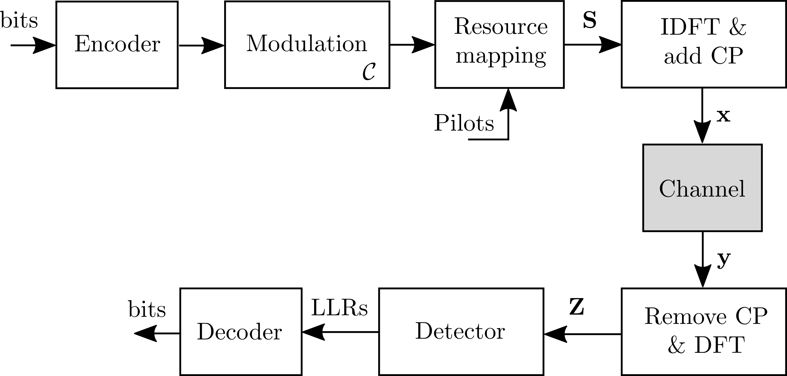
Figure 1: OFDM-based communication system. Interleaving and deinterleaving are not shown for compactness.

II-A Channel model

An OFDM system is considered and the time-frequency matrix of symbols to transmit is denoted by $\mathbf{S}\in\mathbb{C}^{n_{S}\times n_{T}}$, where $n_{S}$ is the number of subcarriers and $n_{T}$ the number of OFDM symbols forming the resource grid. Depending on the transmission scheme, elements of $\mathbf{S}$ can be either a pilot symbol or a modulated symbol according to a constellation ${\cal C}$, e.g., QAM or a learned constellation. As illustrated in Fig. 1, the transmitted signal $\mathbf{x}$ is obtained by applying the inverse discrete Fourier transform (IDFT) to $\mathbf{S}$ and adding a CP, which can be formally written as

$$\mathbf{x}=\text{vec}\left(\mathbf{C_{T}}\mathbf{F}_{n_{S}}^{\mathsf{H}}\mathbf{S}\right)$$ (1)

where $\mathbf{C_{T}}\in\mathbb{C}^{(n_{S}+n_{CP})\times n_{S}}$ is the operator corresponding to the addition of the CP, $n_{CP}$ being the CP length. More precisely,

$$\mathbf{C_{T}}\coloneqq\left[\begin{array}[]{c}\begin{array}[]{cc}\mathbf{0}_{n_{CP}\times(n_{S}-n_{CP})}&\mathbf{I}_{n_{CP}}\end{array}\\ \mathbf{I}_{n_{S}}\end{array}\right].$$ (2)

The scheme presented in Section III does not require the use of a CP, i.e., $n_{CP}=0$ and $\mathbf{C_{T}}=\mathbf{I}_{n_{S}}$.

We consider a multi-tap and time varying channel with $n_{R}$ taps. Elements of the channel output $\mathbf{y}\in\mathbb{C}^{(n_{S}+n_{CP})n_{T}}$ are given by

$$y_{t}=\sum_{i=0}^{n_{R}-1}x_{t-i}h_{i,t}+w_{t}$$ (3)

where $h_{i,t}\in\mathbb{C}$ is the channel coefficient for the $i^{\text{th}}$ tap at time step $t$, and $w_{t}\in\mathbb{C}$ the additive white complex Gaussian noise with variance $\sigma^{2}$. The transmitted symbols are assumed to have an average energy equal to one, i.e., ${\mathbb{E}}\left\{\left|x_{t}\right|^{2}\right\}=1$.

At the receiver, the signal $\mathbf{y}$ is first reshaped as a matrix $\mathbf{Y}\in\mathbb{C}^{(n_{S}+n_{CP})\times n_{T}}$. The CP is then removed and the DFT is applied to obtain

$$\mathbf{Z}=\mathbf{F}_{n_{S}}\mathbf{C_{R}}\text{vec}^{-1}\left(\mathbf{y}\right)$$ (4)

where $\mathbf{C_{R}}\coloneqq\left[\mathbf{0}_{n_{S}\times n_{CP}}\mathbf{I}_{n_{S}}\right]$. If no CP is used, then $\mathbf{C_{R}}=\mathbf{I}_{n_{S}}$. The effective transfer function in the time-frequency domain is

$$\mathbf{z}=\mathbf{G}\mathbf{s}+\mathbf{w}$$ (5)

where $\mathbf{z}\coloneqq\text{vec}\left(\mathbf{Z}\right)$, $\mathbf{s}\coloneqq\text{vec}\left(\mathbf{S}\right)$, and $\mathbf{w}$ is a vector of white Gaussian noise with variance $\sigma^{2}$ per element. The channel matrix $\mathbf{G}\in\mathbb{C}^{n\times n}$, with $n\coloneqq n_{S}n_{T}$, is

$$\mathbf{G}=\left(\mathbf{I}_{n_{T}}\otimes\left(\mathbf{F}_{n_{S}}\mathbf{C_{R}}\right)\right)\mathbf{H}\left(\mathbf{I}_{n_{T}}\otimes\left(\mathbf{C_{T}}\mathbf{F}_{n_{S}}^{\mathsf{H}}\right)\right)$$ (6)

where $\mathbf{H}\in\mathbb{C}^{n_{T}\left(n_{CP}+n_{S}\right)\times n_{T}\left(n_{CP}+n_{S}\right)}$, is the channel matrix in time domain composed of the channel taps.

Because a time-varying channel is assumed, $\mathbf{G}$ is non-diagonal in general. Therefore, we rewrite the transfer function (5) as

$$\mathbf{z}=\text{diag}\left(\mathbf{g}\right)\mathbf{s}+\left(\mathbf{G}-\text{diag}\left(\mathbf{g}\right)\right)\mathbf{s}+\mathbf{w}$$ (7)

where $\mathbf{g}\in\mathbb{C}^{n}$ is the diagonal of $\mathbf{G}$. The first term on the right-hand side of (7) corresponds to the single-tap coefficients, whereas the second term accounts for the inter-carrier interference (ICI) due to the time-varying channel coefficients, as well as for ISI if $n_{CP}\leq n_{R}-1$.

As shown in Fig. 1, $\mathbf{Z}$ is processed by a detector that computes LLRs for the transmitted coded bits, which are then fed to a channel decoder that reconstructs the transmitted bits. The rest of this section presents a baseline for such a detector, which performs LMMSE channel estimation based on transmitted pilots, followed by soft-demapping assuming Gaussian noise, as illustrated in Fig. 2.

II-B LMMSE channel estimation and Gaussian demapping

Figure 2: Architecture of the detector baseline.

The considered baseline assumes a single-tap time-frequency channel, i.e., $\left(\mathbf{G}-\text{diag}\left(\mathbf{g}\right)\right)=\mathbf{0}_{n\times n}$, so that

$$\mathbf{z}=\text{diag}\left(\mathbf{g}\right)\mathbf{s}+\mathbf{w}.$$ (8)

This is equivalent to assuming no ICI. Note that this is neither true in practical channels nor in the channel model depicted in Section II-A. However, this is a quite usual assumption as it enables convenient single-tap equalization. Let us denote by $\mathbf{R}\in\mathbb{C}^{n\times n}$ the covariance matrix of $\mathbf{g}$. The matrix $\mathbf{R}$ determines the temporal and spectral correlation of the OFDM channel.

We denote by $\mathbf{P}\in\mathbb{C}^{n_{S}\times n_{T}}$ the pilot matrix, whose entry $P_{i,k}$ is zero if the RE on the $i^{th}$ subcarrier and $k^{th}$ time slot is carrying data, or equal to the pilot value otherwise. Let $n_{P}$ be the number of pilot-carrying REs which are considered for channel estimation. For these REs, we can re-write (8) considering only the pilots in vectorized form as

$$\mathbf{z_{P}}=\mathbf{\Pi}\left(\text{diag}(\mathbf{p})\mathbf{g}+\mathbf{w}\right)$$ (9)

where $\mathbf{p}\coloneqq\text{vec}(\mathbf{P})$, and $\mathbf{\Pi}$ is the $n_{P}\times n$ matrix which selects only the elements carrying pilot symbols. Assuming knowledge of $\mathbf{R}$ at the receiver, the LMMSE channel estimate is (e.g., [7, Lemma B.17])

$$\widehat{\mathbf{g}}=\mathbf{R}\text{diag}(\mathbf{p})^{\mathsf{H}}\mathbf{\Pi}^{\mathsf{H}}\cdot\\ \left(\mathbf{\Pi}\left(\text{diag}(\mathbf{p})\mathbf{R}\text{diag}(\mathbf{p})^{\mathsf{H}}+\sigma^{2}\mathbf{I}_{n}\right)\mathbf{\Pi}^{\mathsf{H}}\right)^{-1}\mathbf{z_{p}}.$$ (10)

Using this result, the received signal, which incorporates both pilots and data, can be re-written in vector form as

$$\mathbf{z}=\text{diag}(\widehat{\mathbf{g}})\mathbf{s}+\underbrace{\text{diag}(\widetilde{\mathbf{g}})\mathbf{s}+\mathbf{w}}_{\coloneqq\widetilde{\mathbf{w}}}$$ (11)

where $\widetilde{\mathbf{g}}=\mathbf{g}-\widehat{\mathbf{g}}$ is the channel estimation error with correlation matrix $\widetilde{\mathbf{R}}\in\mathbb{C}^{n\times n}$, given as

$$\widetilde{\mathbf{R}}={\mathbb{E}}\left\{\widetilde{\mathbf{g}}\widetilde{\mathbf{g}}^{\mathsf{H}}\right\}=\mathbf{R}-\mathbf{R}\text{diag}(\mathbf{p})^{\mathsf{H}}\mathbf{\Pi}^{\mathsf{H}}\\ \left(\mathbf{\Pi}\left(\text{diag}(\mathbf{p})\mathbf{R}\text{diag}(\mathbf{p})^{\mathsf{H}}+\sigma^{2}\mathbf{I}_{n}\right)\mathbf{\Pi}^{\mathsf{H}}\right)^{-1}\mathbf{\Pi}\text{diag}(\mathbf{p})\mathbf{R}$$ (12)

and $\widetilde{\mathbf{w}}$ is the sum of noise and residual interference due to imperfect channel estimation.

Soft-demapping is performed assuming that $\widetilde{\mathbf{w}}$ is Gaussian. Let us denote by $m$ the number of bits per channel use, by ${\cal C}=\{c_{1},\dots,c_{2^{m}}\}$ the constellation, and by ${\cal C}_{i,0}$ (${\cal C}_{i,1}$) the subset of ${\cal C}$ which contains all constellation points with the $i^{th}$ bit label set to 0 (1). The LLR for the $i^{th}$ bit ($i\in\{1,\dots,m\}$) of the $k^{th}$ RE ($k\in\{1,\dots,n\}$) is computed as follows:

$$\text{LLR}(k,i)=\mathop{\mathrm{ln}}\left(\frac{\sum_{c\in{\cal C}_{i,1}}\mathop{\mathrm{exp}}\left(-\frac{1}{\widetilde{\sigma}_{k}^{2}}\left|z_{k}-\widehat{g}_{k}c\right|^{2}\right)}{\sum_{c\in{\cal C}_{i,0}}\mathop{\mathrm{exp}}\left(-\frac{1}{\widetilde{\sigma}_{k}^{2}}\left|z_{k}-\widehat{g}_{k}c\right|^{2}\right)}\right)$$ (13)

where $\widetilde{\sigma}_{k}^{2}={\mathbb{E}}\left\{\widetilde{w}_{k}\widetilde{w}_{k}^{*}\right\}=\widetilde{R}_{k,k}+\sigma^{2}$ for $k=1,\dots,n$. Whenever $k$ corresponds to the index of a pilot symbol, no LLR value is computed. After deinterleaving, the LLRs are fed to a channel decoding algorithm (e.g., belief propagation) which computes predictions of the transmitted bits.

III End-to-end learning for OFDM

End-to-end learning of communication systems [3] consists in implementing a transmitter, channel, and receiver as a single NN referred to as an autoencoder, and jointly optimizing the trainable parameters of the transmitter and receiver for a specific channel model. In our setting, training aims at minimizing the total binary cross-entropy (BCE)$\mathrm{bit}\text{\,}{\mathrm{frame}}^{-1}$, defined as

$${\cal L}\coloneqq-\sum_{k\in{\cal N}_{D}}\sum_{i=1}^{m}{\mathbb{E}}_{b_{k,i},\mathbf{z}}\left\{\mathop{\mathrm{log}}\left(Q_{k,i}\left(b_{k,i}|\mathbf{z}\right)\right)\right\}$$ (14)

where ${\cal N}_{D}$ is the set of size $n_{D}$ of indexes of REs carrying data symbols, $b_{k,i}$ is the $i^{th}$ bit transmitted in the $k^{th}$ resource element, and $Q_{k,i}\left(\cdot|\mathbf{z}\right)$ is the receiver estimate of the posterior distribution of the $i^{th}$ bit transmitted in the $k^{th}$ RE, given the received signal after OFDM demodulation $\mathbf{z}$. Since (14) is numerically difficult to compute, it is estimated through Monte Carlo sampling as

$${\cal L}\approx-\frac{1}{S}\sum_{l=1}^{S}\sum_{k\in{\cal N}_{D}}\sum_{i=1}^{m}\left\{\mathop{\mathrm{log}}\left(Q_{k,i}\left(b_{k,i}^{[l]}|\mathbf{z}^{[l]}\right)\right)\right\}$$ (15)

where $S$ is the batch size, i.e., the number of samples used to estimate ${\cal L}$, and the superscript $[l]$ is used to refer to the $l^{th}$ sample within a batch. Interestingly, as proved in [8], minimzing ${\cal L}$ is equivalent to maximizing an achievable rate, assuming that a mismatched bit-metric decoding (BMD) receiver is used.

Training of the transmitter typically involves joint optimization of the constellation geometry and bit labeling [2]. Such an approach is adopted in this work and extended to OFDM channels in Section III-A. Moreover, a centered constellation is learned, assuming that no pilots are transmitted and no CP is used, as shown in Fig. 3. This avoids an unwanted DC offset and removes the throughput loss due to the transmission of reference signals and CP that carry no data. The architecture of the NN-based receiver is detailed in Section III-B.

III-A Learning of geometric shaping and bit-labeling

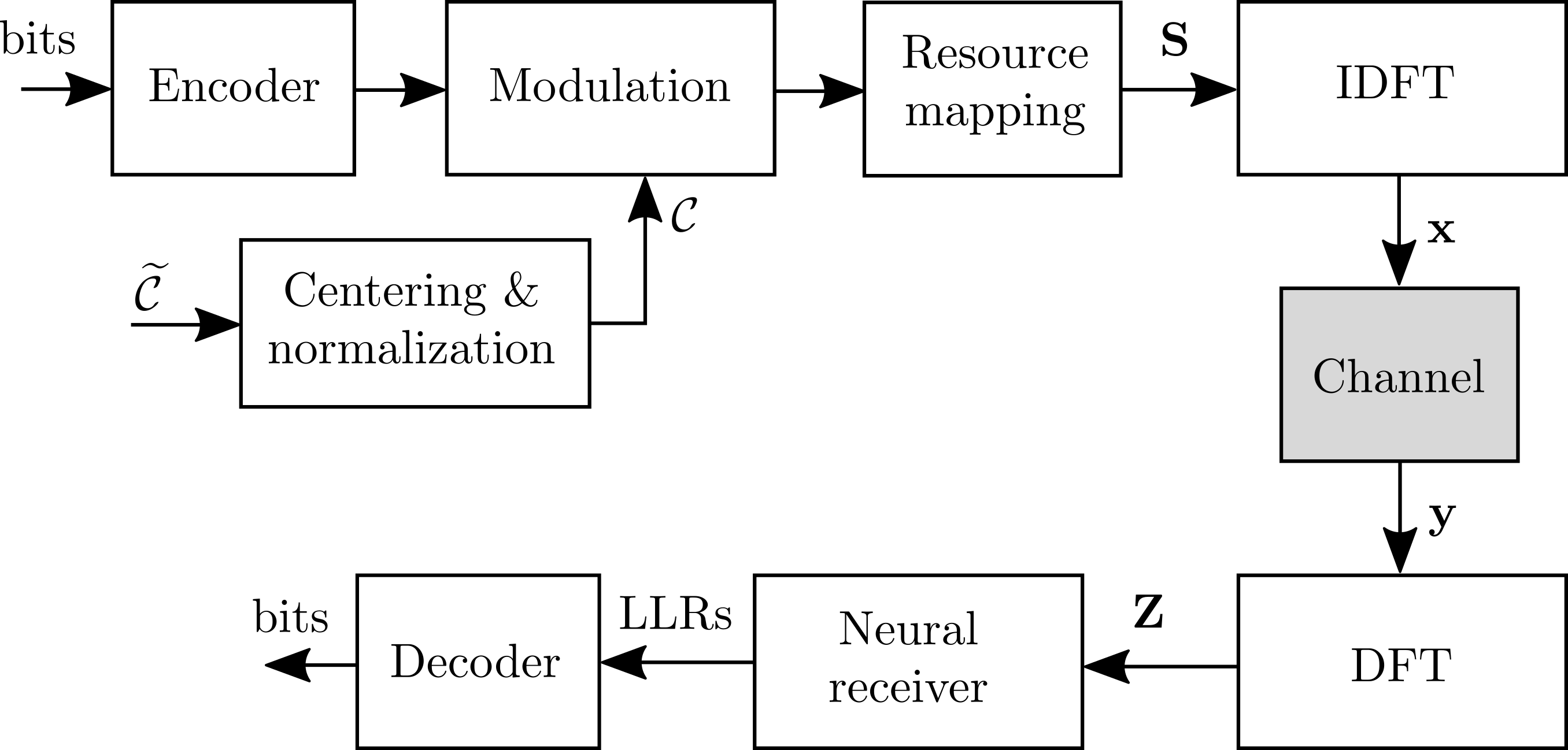
Figure 3: End-to-end learning system.

The system architecture we have adopted in this work is depicted in Fig. 3. On the transmitter side, the trainable parameters consist of a set denoted by $\widetilde{{\cal C}}$ of $2^{m}$ complex numbers corresponding to the constellation points. The constellation used for transmitting data is obtained by centering and normalizing $\widetilde{{\cal C}}$, i.e.,

$${\cal C}=\frac{\widetilde{{\cal C}}-\frac{1}{2^{m}}\sum_{c\in\widetilde{{\cal C}}}c}{\sqrt{\frac{1}{2^{m}}\sum_{c\in\widetilde{{\cal C}}}\left|c\right|^{2}-\left|\frac{1}{2^{m}}\sum_{c\in\widetilde{{\cal C}}}c\right|^{2}}}.$$ (16)

Normalization of the constellation ensures that it has unit average power, while centering forces the constellation to have zero mean and prevents learning of embedded superimposed pilots. As no pilots are transmitted, the receiver can only exploit the constellation geometry to reconstruct the transmitted bits and mitigate ISIs due to the lack of CP and ICIs due to Doppler spread. Compared to previous work such as [2], a single constellation is learned, which is used for all signal-to-noise ratios (SNRs), Doppler, and delay spreads. On the receiver side, an NN that operates on multiple subcarriers and OFDM symbols is leveraged, whose architecture is detailed in Section III-B. As in [2], training of the end-to-end systems is done on the total BCE estimated by (15).

III-B Receiver architecture

(a) Architecture of the neural receiver.

(b) Architecture of a ResNet block.

Figure 4: The receiver is implemented by a residual convolutional neural network.

The architecture of the NN implementing the receiver is shown in Fig. 4. It is a convolutional residual NN [9] that takes as input the received baseband channel samples after the DFT $\mathbf{Z}$ of dimension $n_{S}\times n_{T}$, and outputs a 3-dimensional tensor of LLRs of dimension $n_{S}\times n_{T}\times m$ that is fed to the channel decoder. The NN hence substitutes the estimator and demapper shown in Fig. 2. The first layer $\mathbb{C}2\mathbb{R}$ converts the complex-valued input tensor of dimension $n_{S}\times n_{T}$ into a real-valued 3-dimensional tensor of dimension $n_{S}\times n_{T}\times 2$ by stacking the real and imaginary parts into an additional dimension. Separable convolutional layers are used to reduce the number of weights, without incurring significant loss of performance. Table I provides details on the NN implementing the receiver. All convolutional layers use zero-padding to ensure that the dimensions of the output are the same as the ones of the input. Dilation is leveraged to increase the receptive field of the convolutional layers. A similar but somewhat larger architecture was used in [10].

Layer	Channels	Kernel size	Dilatation rate
Input Conv2D	256	(3,3)	(1,1)
ResNet block 1	256	(3,3)	(3,1)
ResNet block 2	256	(3,3)	(6,2)
ResNet block 3	256	(3,3)	(6,2)
ResNet block 4	256	(3,3)	(3,1)
Output Conv2D	$m$	(1,1)	(1,1)

TABLE I: Architecture details of the NN implementing the receiver.

(a) Pilot pattern “1P”.

(b) Pilot pattern “2P”.

Figure 5: Pilot patterns from 5G NR used in simulations.

IV Simulation results

We will now present the results of the simulations we have conducted to evaluate the machine learning-based scheme introduced in the previous section, referred to as the geometric shaping (GS) scheme. We start by explaining the training and evaluation setup. The GS scheme is then compared to several other baselines.

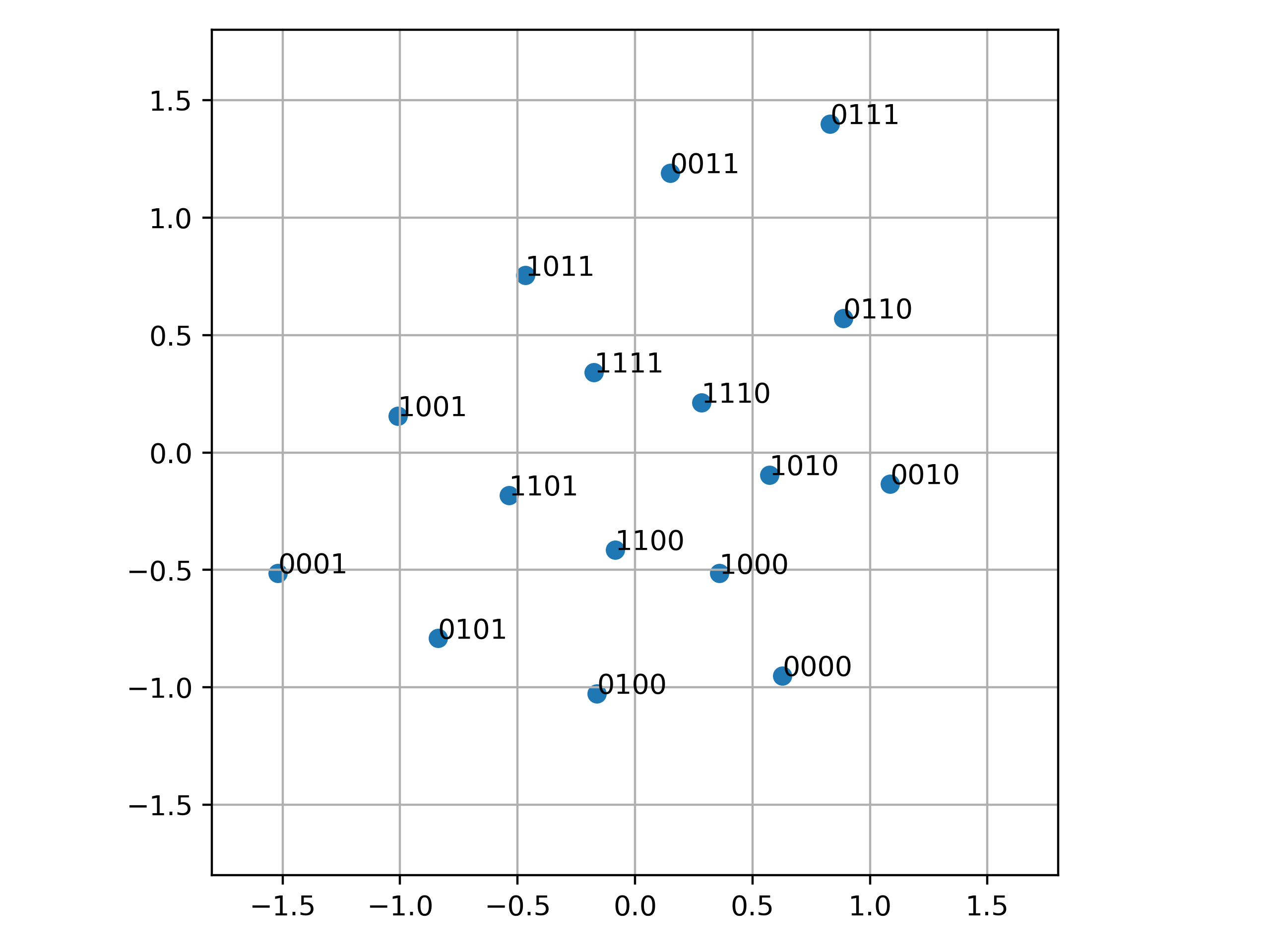
Figure 6: Learned constellation geometry and labeling.

IV-A Evaluation setup

Parameter	Symbol (if any)	Value
Number of OFDM symbols	$n_{T}$	14 (1 slot)
Number of subcarriers	$n_{S}$	72 (6 PRBs)
Frequency carrier	(None)	$3.5\text{\,}\mathrm{GHz}$
Subcarrier spacing	(None)	$30\text{\,}\mathrm{kHz}$
Cycle prefix duration	$n_{CP}$	6 symbols (5G NR CP of $2.34\text{\,}\mathrm{\SIUnitSymbolMicro s}$)
Channel models	(None)	3GPP-3D LoS and NLoS
Number of taps	$n_{R}$	5
Learning rate	(None)	$10^{-3}$
Batch size for training	$S$	100 frames
Bit per channel use	$m$	$4\text{\,}\mathrm{bit}$
Code length	(None)	$1024\text{\,}\mathrm{bit}$
Code rate	$r$	$\frac{2}{3}$
Speed range used for training	(None)	$0$ to $130\text{\,}\mathrm{km}\text{\,}{\mathrm{h}}^{-1}$

TABLE II: Parameters used for training and evaluation

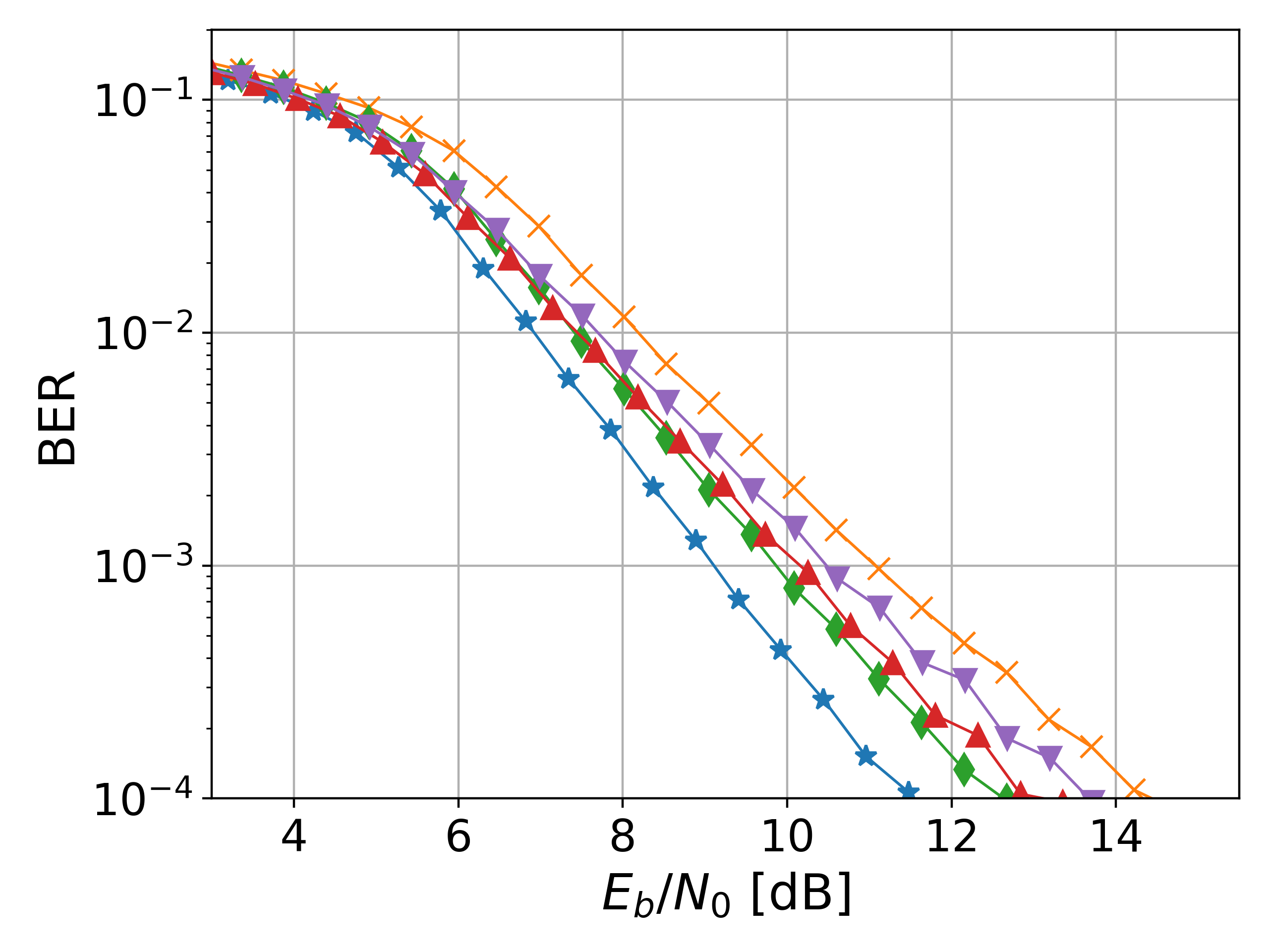
(a) 1P & Low speed: 3.6$\mathrm{km}\text{\,}{\mathrm{h}}^{-1}$.

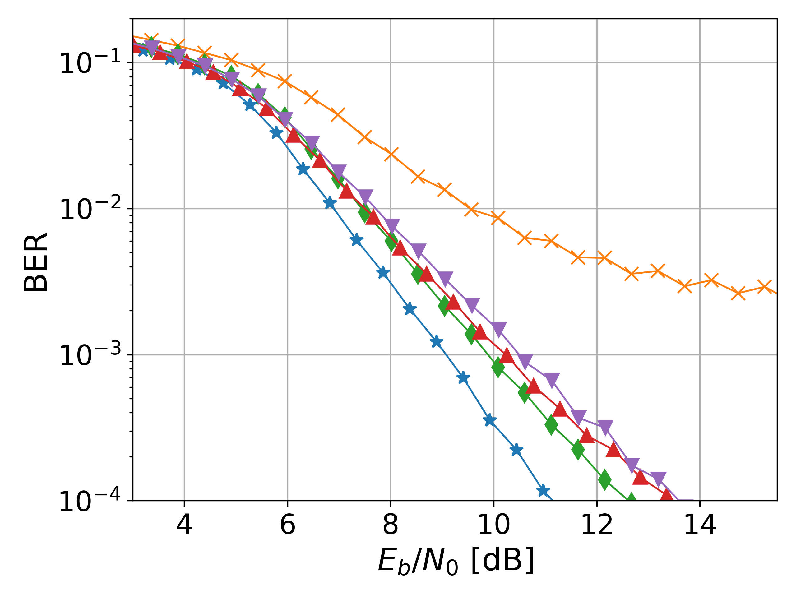
(b) 1P & Medium speed: 36$\mathrm{km}\text{\,}{\mathrm{h}}^{-1}$.

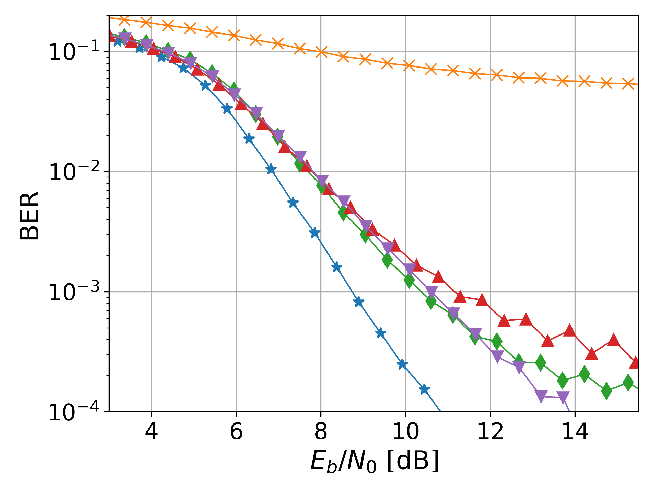
(c) 1P & High speed: 108$\mathrm{km}\text{\,}{\mathrm{h}}^{-1}$.

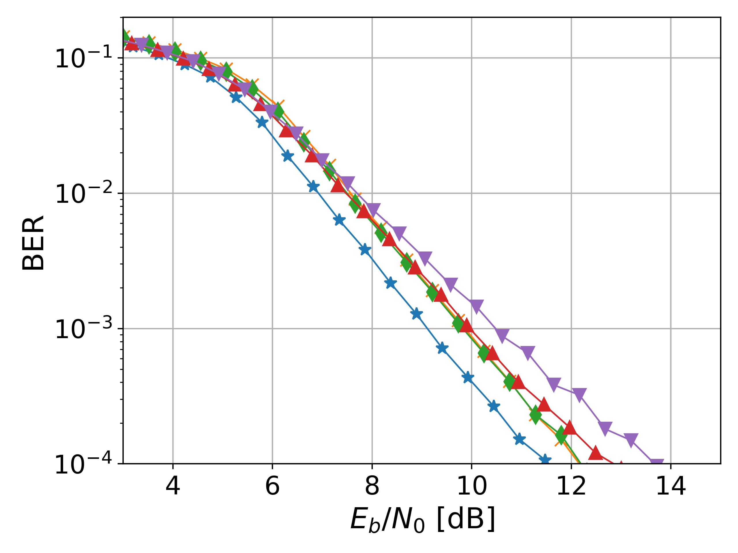
(d) 2P & Low speed: 3.6$\mathrm{km}\text{\,}{\mathrm{h}}^{-1}$.

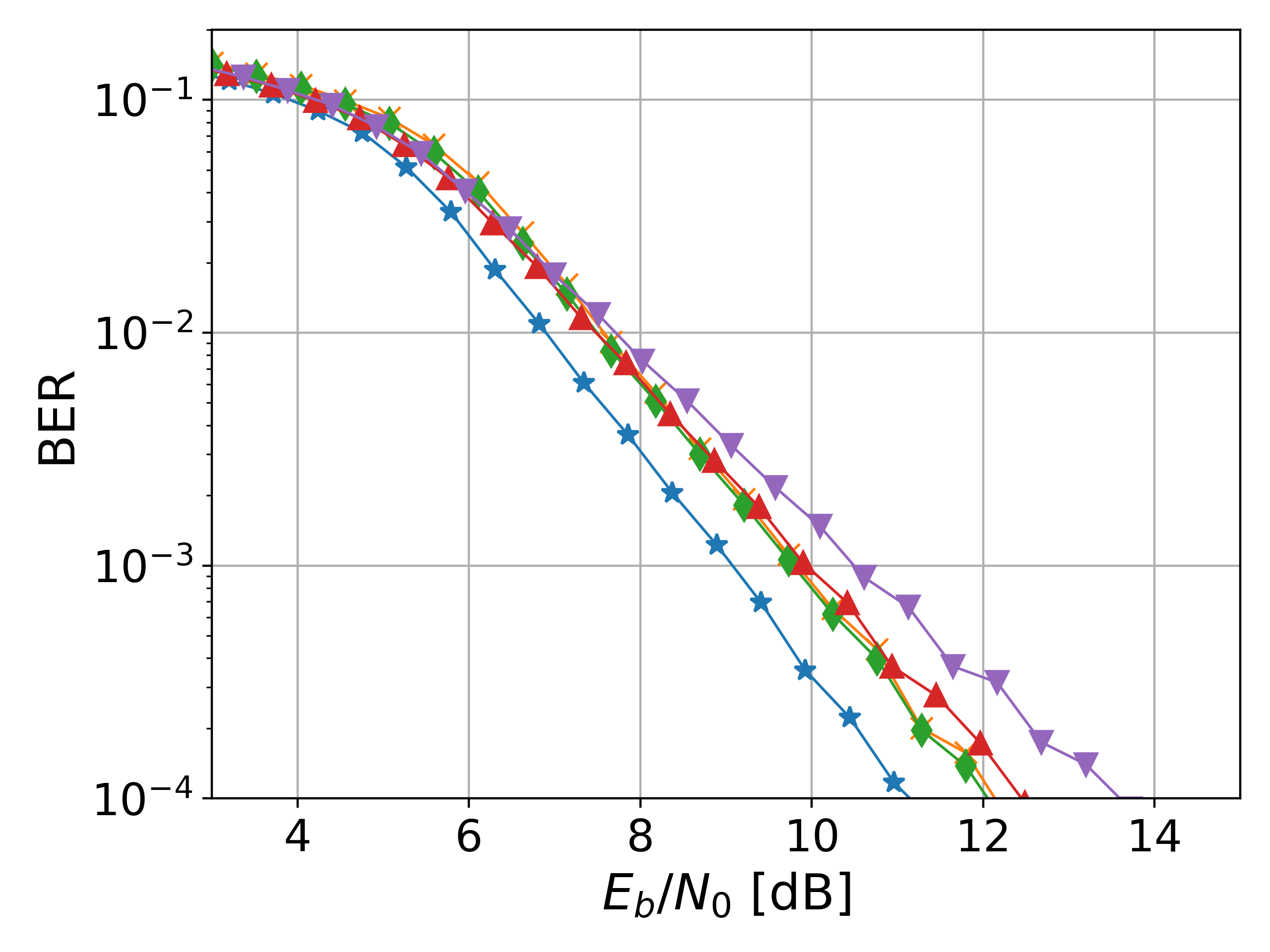
(e) 2P & Medium speed: 36$\mathrm{km}\text{\,}{\mathrm{h}}^{-1}$.

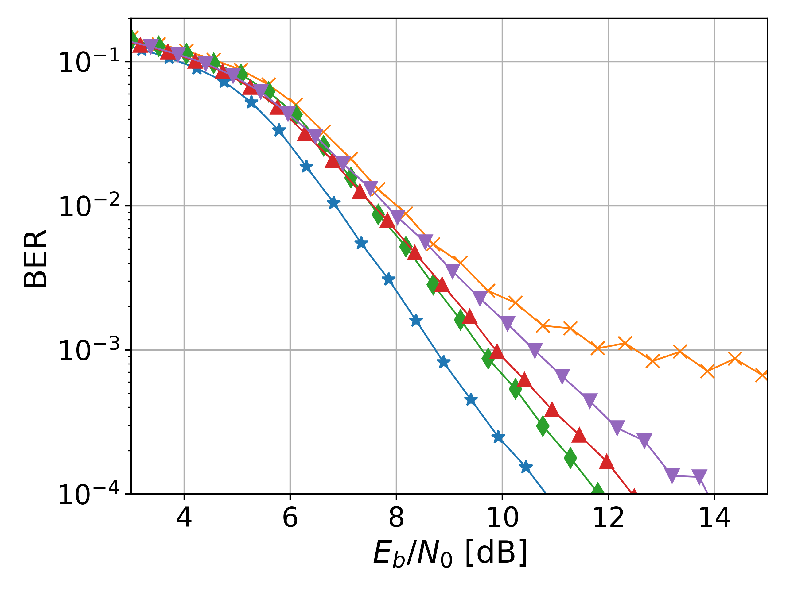
(f) 2P & High speed: 108$\mathrm{km}\text{\,}{\mathrm{h}}^{-1}$.

Figure 7: BER achieved by the different schemes.

The channel model introduced in Section II-A was considered to train the end-to-end system and to evaluate it against multiple baselines. In addition to the LMMSE baseline introduced in Section II-B, a receiver that assumes (8) as transfer function and has perfect knowledge of $\mathbf{g}$ was also considered. A scheme that leverages the neural receiver from Section III-B with QAM, pilots, and CP was also considered, as well as an approach that leverages the neural receiver and QAM but without CP. Table II shows the parameters used to train and evaluate the machine learning-based approaches. Training was done over the speed range from $0$ to $130\text{\,}\mathrm{km}\text{\,}{\mathrm{h}}^{-1}$. The 3rd Generation Partnership Project (3GPP) UMi LoS and NLoS channel models were considered, and the Quadriga [11] simulator was used to generate a dataset used to train and evaluate the considered approaches. The energy per bit to noise power spectral density ratio is

$$\frac{E_{b}}{\sigma^{2}}\coloneqq\frac{1}{\rho}\frac{1}{mr\sigma^{2}}$$ (17)

assuming ${\mathbb{E}}\left\{\left|X_{i,k}\right|^{2}\right\}=1$ for all REs $(i,k)$, and where $\rho$ is the ratio of symbols carrying data (the rest of the being used for pilots and CP) and $r$ is the code rate. Two pilot patterns from 5G NR were considered, which are shown in Fig. 5. The first one has pilots on only one OFDM symbol (Fig. 5(a)), whereas the second one has extra pilots on a second OFDM symbol (Fig. 5(b)), which makes it more suitable to high mobility scenarios. These two pilot patterns are referred to as “1P” and “2P”, respectively.

A standard 5G NR low-density parity-check (LDPC) code of length $1024\>$bit and with rate $\frac{2}{3}$ was used. Decoding was done with conventional belief-propagation, using 40 iterations. Each transmitted OFDM frame contained 3 codewords and was filled up with randomly generated padding bits. Interleaving was performed within individual frames.

The NN-based receiver operates on the entire frame. For fairness, the channel estimation (10) is also performed on the entire frame. This involves the multiplication and inversion of matrices of dimension $1008\times 1008$. Moreover, it requires knowledge of the channel correlation matrix $\mathbf{R}$, which depends on the the Doppler and delay spread. However, the receiver typically does not have access to this information, and assuming it to be available would lead to an unfair comparison with the NN-based receiver which is not fed with the Doppler and delay spread. Therefore, a unique correlation matrix has been estimated using the training set. The so-obtained correlation matrix estimate was used to implement the LMMSE baseline.

IV-B Evaluation of end-to-end learning

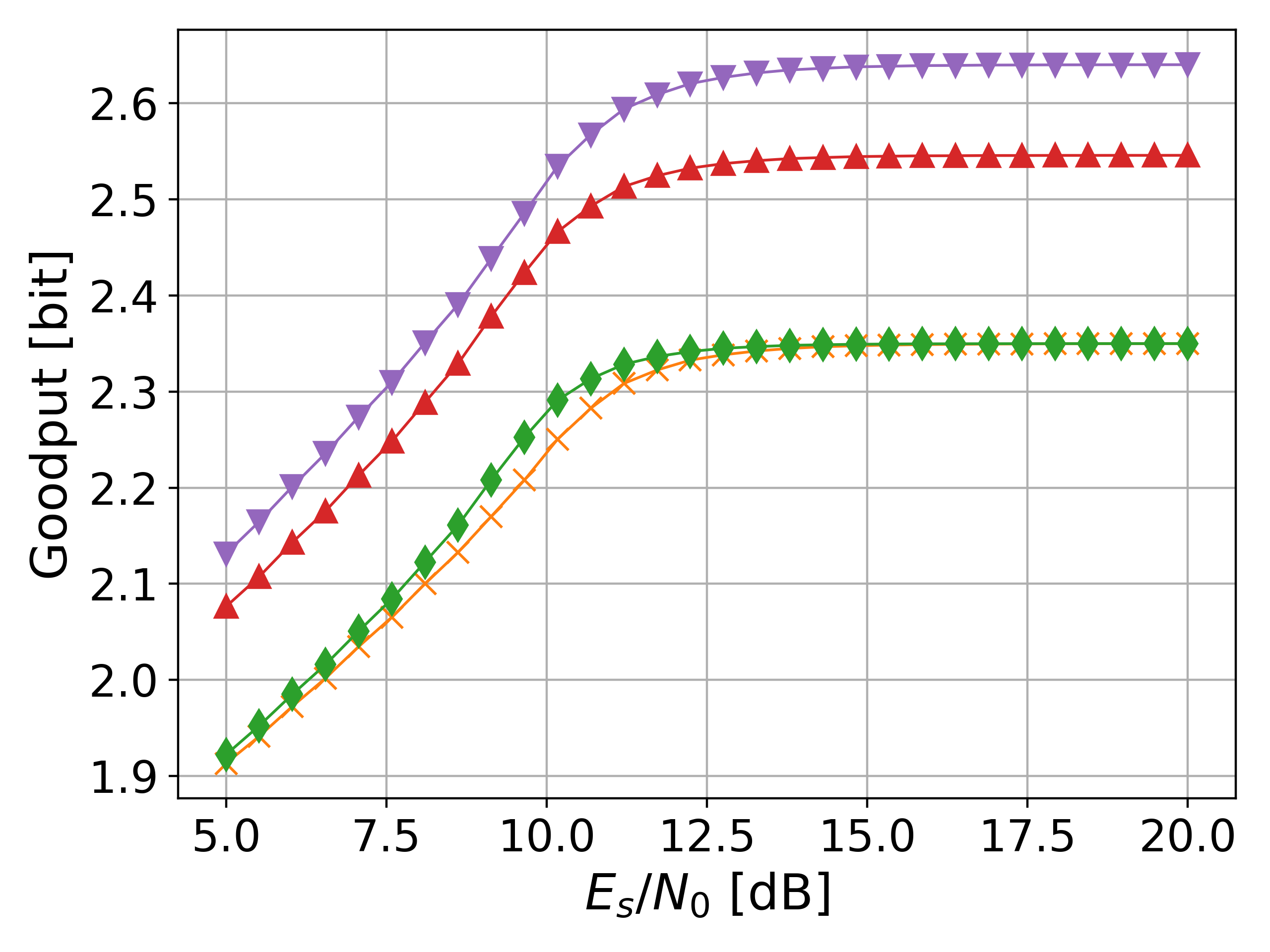
(a) 1P & Low speed: 3.6$\mathrm{km}\text{\,}{\mathrm{h}}^{-1}$.

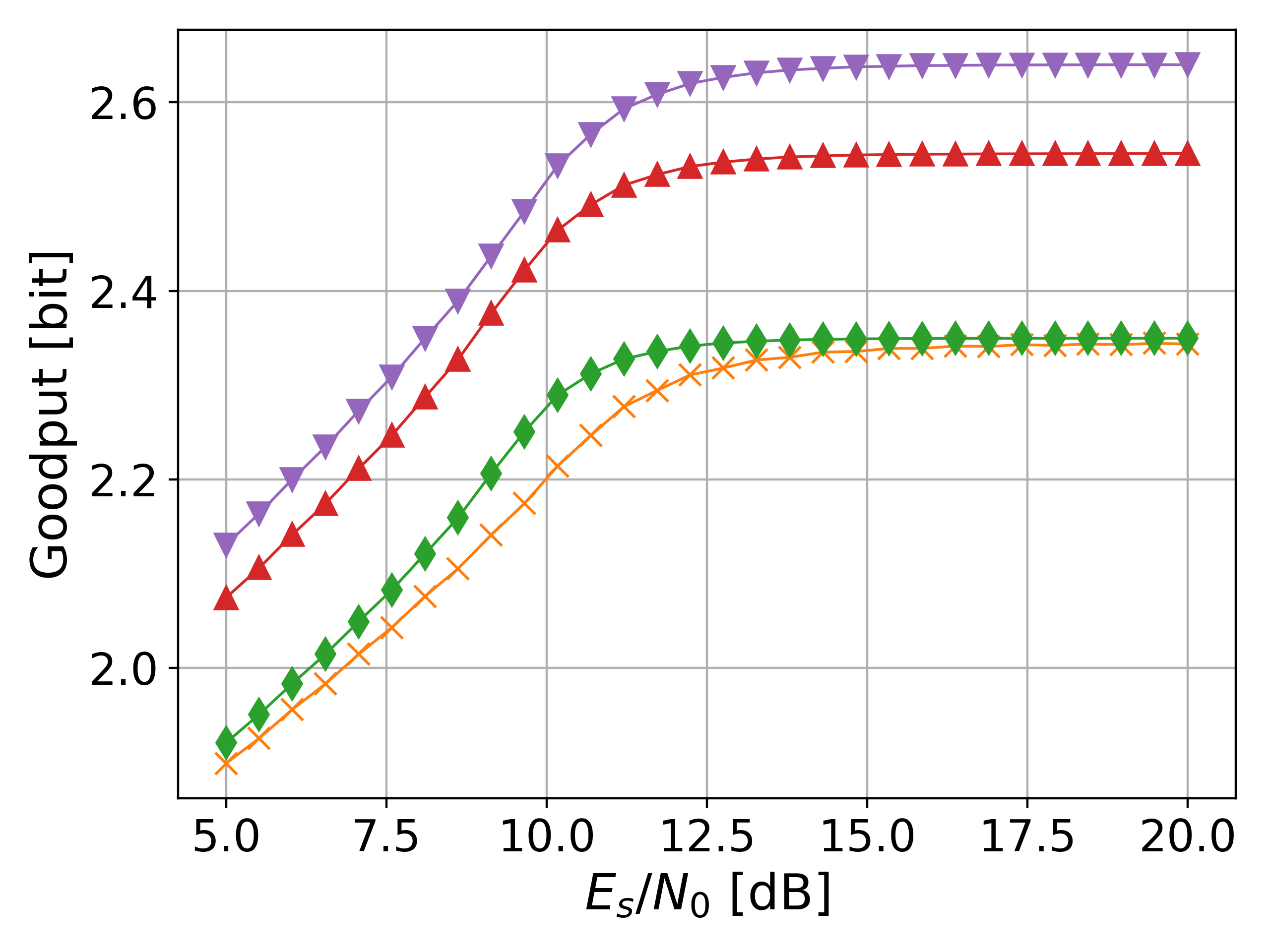
(b) 1P & Medium speed: 36$\mathrm{km}\text{\,}{\mathrm{h}}^{-1}$.

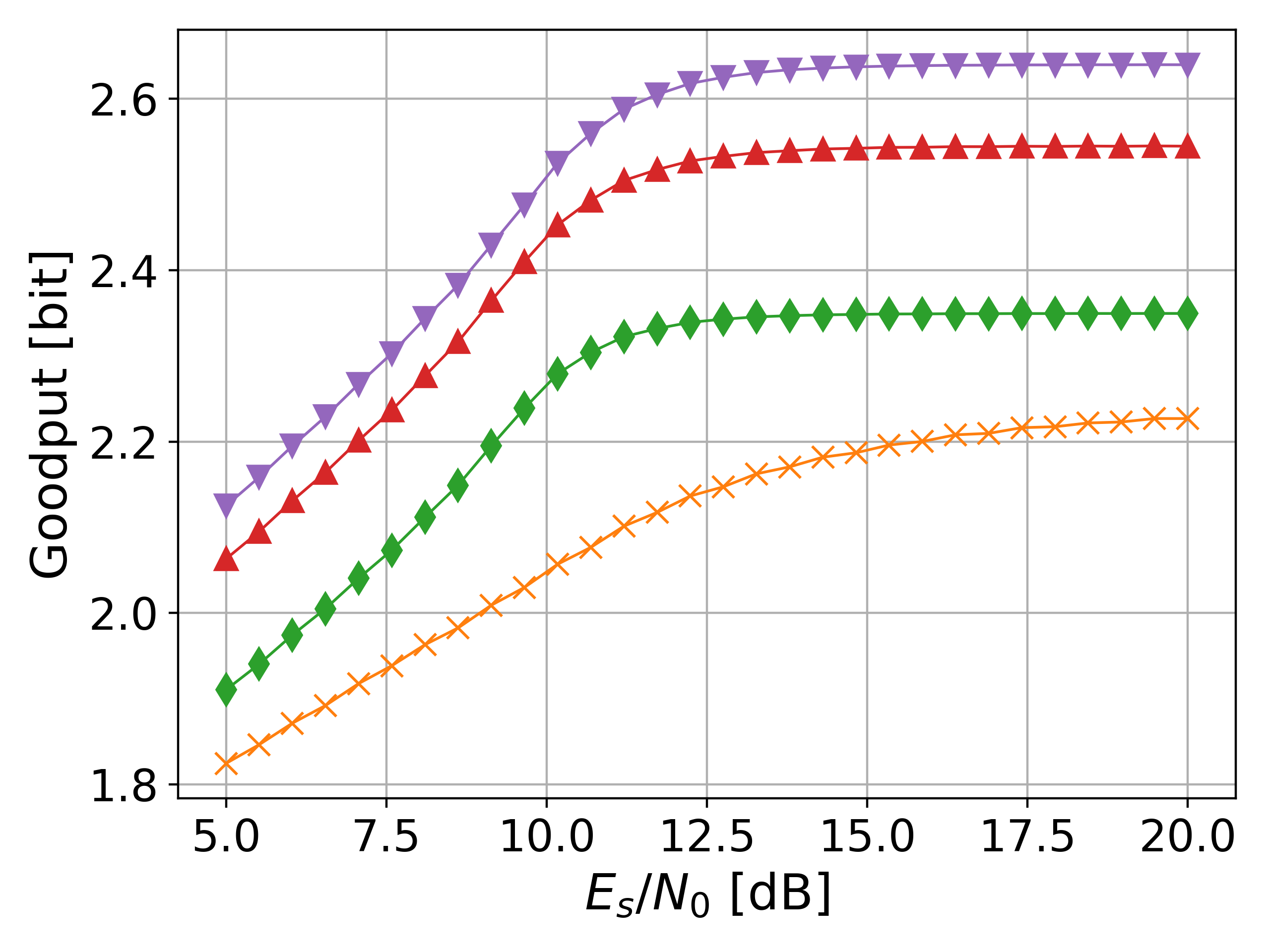
(c) 1P & High speed: 108$\mathrm{km}\text{\,}{\mathrm{h}}^{-1}$.

(d) 2P & Low speed: 3.6$\mathrm{km}\text{\,}{\mathrm{h}}^{-1}$.

(e) 2P & Medium speed: 36$\mathrm{km}\text{\,}{\mathrm{h}}^{-1}$.

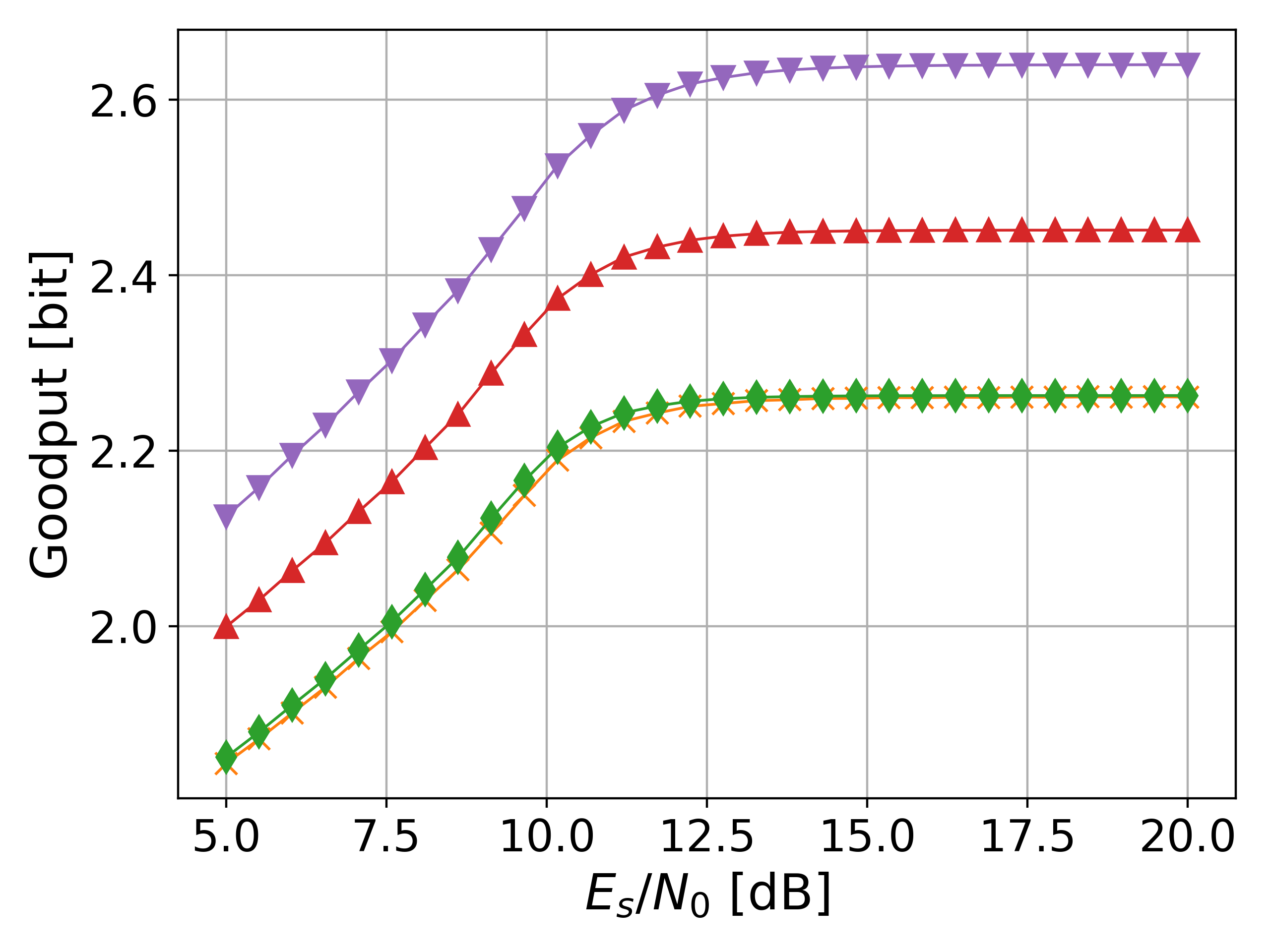
(f) 2P & High speed: 108$\mathrm{km}\text{\,}{\mathrm{h}}^{-1}$.

Figure 8: Goodput achieved by the different schemes.

Fig. 6 shows the constellation and labeling obtained by training the end-to-end system introduced in Section III. One can see that the learned constellation has a unique axis of symmetry. Moreover, a form of Gray labeling was learned, such that points next to each other differ by one bit.

The first row in Fig. 7 shows the BERs achieved by the various schemes when the 1P pilot pattern is used for three different velocities. Note that the GS scheme does not use any pilots. One can see that the LMMSE-based baseline leads to the highest BERs for all speeds. Moreover, its BERs significantly worsen as the speed increases. The lowest BERs are achieved by the neural receiver with QAM, pilots, and CP. The GS scheme and the approach leveraging the neural receiver with QAM, pilots, but without CP achieve similar BERs for the low and medium speeds, slightly higher than the one achieved by the neural receiver with QAM, pilots, and CP. However, at high speed, the systems leveraging the neural receiver, QAM, and pilots decline whereas the GS scheme is more robust and achieves the lowest BERs.

The second row in Fig. 7 shows the achieved BERs when leveraging the 2P pilot pattern. As expected, using more pilots enables the schemes using them to achieve lower BERs, except for the LMMSE baseline. However, this is at the cost of extra pilots, leaving less resources to transmit data-carrying symbols. The benefits of achieving low BERs without the requirement of transmitting pilots and CP, as allowed by the GS scheme, is that it enables higher goodput, as shown in Fig. 8. The baseline assuming perfect channel knowledge was omitted for clarity. The goodput measures the average number of bits per symbols successfully received, and is defined by

$$\text{Goodput}\coloneqq r\rho m\left(1-\text{BER}\right)$$ (18)

where $\rho$ is the ratio of data carrying symbols. Moreover, because the goodput accounts for the unequal average number of information bits transmitted per symbol among the different schemes through the parameter $\rho$, it is plotted with respect to the energy per symbol to noise power spectral density ratio, defined as $\frac{E_{s}}{\sigma^{2}}\coloneqq\frac{1}{\sigma^{2}}$. These plots show that the end-to-end approach enables at least $18\text{\,}\mathrm{\char 37\relax}$ gains over the LMMSE-based baseline (Fig. 8(f)), and at least $4\text{\,}\mathrm{\char 37\relax}$ gains over the neural receiver with QAM, pilots, but no CP. One can see that for all the considered speeds and pilot patterns, the GS scheme achieves the highest goodput. The pilot and CP-based schemes saturate at lower values as some of the symbols are not transmitting data.

V Conclusion

We have investigated the performance of end-to-end learning on top of OFDM, and have shown that end-to-end learning enables multi-carrier communication without the need for CP or pilots, and without significant loss of BER. This enables significant gains in throughput, as more resources are available for transmitting data. Moreover, the learned system works for both line-of-sight (LoS) and non-LoS, and for a wide range of speeds and SNRs. Thus, apart from throughput gains, pilotless transmissions could remove the control signaling overhead related to the choice of the best suitable pilot pattern and CP.

References

- [1] H. Viswanathan and P. E. Mogensen, “Communications in the 6g era,” IEEE Access, vol. 8, pp. 57 063–57 074, 2020.
- [2] S. Cammerer, F. Ait Aoudia, S. Dörner, M. Stark, J. Hoydis, and S. T. Brink, “Trainable Communication Systems: Concepts and Prototype,” IEEE Trans. Commun., 2020.
- [3] T. O’Shea and J. Hoydis, “An Introduction to Deep Learning for the Physical Layer,” IEEE Trans. Cogn. Commun. Netw., vol. 3, no. 4, pp. 563–575, Dec. 2017.
- [4] Z. Zhu, J. Zhang, R. Chen, and H. Yu, “Autoencoder-Based Transceiver Design for OWC Systems in Log-Normal Fading Channel,” IEEE Photon. J., vol. 11, no. 5, pp. 1–12, Oct. 2019.
- [5] B. Karanov, M. Chagnon, F. Thouin, T. A. Eriksson, H. Bülow, D. Lavery, P. Bayvel, and L. Schmalen, “End-to-End Deep Learning of Optical Fiber Communications,” J. Lightw. Technol., vol. 36, no. 20, pp. 4843–4855, Oct. 2018.
- [6] H. Ye, G. Y. Li, and B. Juang, “Power of Deep Learning for Channel Estimation and Signal Detection in OFDM Systems,” IEEE Wireless Commun. Lett., vol. 7, no. 1, pp. 114–117, 2018.
- [7] E. Björnson, J. Hoydis, and L. Sanguinetti, “Massive MIMO networks: Spectral, energy, and hardware efficiency,” Foundations and Trends® in Signal Processing, vol. 11, no. 3-4, pp. 154–655, 2017.
- [8] F. Ait Aoudia and J. Hoydis, “End-to-end Learning for OFDM: From Neural Receivers to Pilotless Communication,” preprint arXiv:2009.05261, 2020.
- [9] K. He, X. Zhang, S. Ren, and J. Sun, “Deep Residual Learning for Image Recognition,” in Proc. IEEE Conf. on Comput. Vision and Pattern Recognit. (CVPR), June 2016.
- [10] M. Honkala, D. Korpi, and J. M. Huttunen, “DeepRx: Fully Convolutional Deep Learning Receiver,” preprint arXiv:2005.01494, 2020.
- [11] Quadriga Radio Channel Generator. [Online]. Available: https://quadriga-channel-model.de/