Towards reliable projections of global mean surface temperature

Abstract

Quantifying the risk of global warming exceeding critical targets such as $2.0\text{\,}\mathrm{K}$ requires reliable projections of uncertainty as well as best estimates of Global Mean Surface Temperature (GMST). However, uncertainty bands on GMST projections are often calculated heuristically and have several potential shortcomings. In particular, the uncertainty bands shown in IPCC plume projections of GMST are based on the distribution of GMST anomalies from climate model runs and so are strongly determined by model characteristics with little influence from observations of the real-world. Physically motivated time-series approaches are proposed based on fitting energy balance models (EBMs) to climate model outputs and observations in order to constrain future projections. It is shown that EBMs fitted to one forcing scenario will not produce reliable projections when different forcing scenarios are applied. The errors in the EBM projections can be interpreted as arising due to a discrepancy in the effective forcing felt by the model. A simple time-series approach to correcting the projections is proposed based on learning the evolution of the forcing discrepancy so that it can be projected into the future. These approaches give reliable projections of GMST when tested in a perfect model setting, and when applied to observations lead to well constrained projections with lower mean warming and narrower projection bands than previous estimates. Despite the reduced uncertainty, the lower warming leads to a greatly reduced probability of exceeding the $2.0\text{\,}\mathrm{K}$ warming target.

1 Introduction

Global Mean Surface Temperature (GMST) is a key quantity for projecting future climate since it integrates many large scale processes, and many changes and impacts scale with GMST (IPCC, 2018; Sutton et al., 2015). It is also the summary measure most often used to communicate climate change to the public and to policy makers. Credible assessments of the risk of global warming exceeding targets such as $2\text{\,}\mathrm{K}$ set out in the Paris agreement are critical for policy makers to make informed decisions about how to meet those targets. Therefore, it is important that the projections such assessments are based on are not only accurate, but also reliable, i.e., the probabilities of particular events are also accurate (Broecker, 2012).

Climate projections are usually derived from general circulation models (GCMs) designed to simulate the climate system as closely as is currently possible (Collins et al., 2013). Uncertainty in climate projections arises from many sources including imprecise initial conditions and natural variability (Deser et al., 2012), the parameters of unresolved processes within a single GCM (Collins, 2007), choices made in constructing one GCM compared to another (Tebaldi and Knutti, 2007), and uncertainty about future emissions. Uncertainty about future emissions is usually addressed by conditioning projections on one or more predetermined scenarios (Moss et al., 2010). Other uncertainties are usually quantified by analysing an ensemble of simulations that vary one or more of the uncertain factors.

The concept behind the use of ensembles for probabilistic projection is that the ensemble members represent samples from the distribution of plausible outcomes (Smith, 2002; Palmer et al., 2006). In practice, limitations of the models, observations etc. affect the spread of the ensemble and reduce the skill of the forecast. This is particularly problematic for multi-model ensembles which are not designed to span a space of possible model constructions, and are often referred to as “ensembles of opportunity” (Knutti et al., 2010; Stephenson et al., 2012). Multi-model projections of GMST in particular exhibit a very large spread of outcomes (Collins, 2007). The IPCC approach to handling this uncertainty is to take anomalies with respect to a specified reference period (Collins, 2007, Figures T.S.14 & T.S.15). This reduces the spread of the projections in the future, but the projected warming and associated uncertainty then depend strongly on the reference period. There is also no reason to believe the projections are probabilistically reliable.

Many methods have been proposed for reducing the uncertainty in multi-model ensemble projections by weighting models according to their past performance in simulating the observed climate (Greene et al., 2006; Min and Hense, 2006; Bhat et al., 2011; Shiogama et al., 2011; Watterson and Whetton, 2011). Some weighting methods have been shown to produce reliable projections of future climate in perfect model tests (Abramowitz and Bishop, 2015; Sanderson et al., 2017; Knutti et al., 2017; Strobach and Bel, 2020). However, others have questioned the use of weights based on past performance when projecting conditions that differ significantly from that past (Stainforth et al., 2007; Sansom et al., 2013). The objection is that all models are fundamentally different from the system they represent and share common limitations that mean perfect model validation imparts only limited confidence. Further, it has been shown that if the weights do not reflect the true model skill, then an unweighted ensemble may be preferred (Weigel et al., 2010).

The alternative to model weighting is to build a formal statistical framework relating climate models to the real-world (Räisänen and Palmer, 2001; Furrer et al., 2007; Buser et al., 2009; Annan and Hargreaves, 2010, 2011). Some statistical frameworks effectively included performance weights of their own (Tebaldi et al., 2005; Smith et al., 2009; Tebaldi and Sansó, 2009). The most recent developments proposed independently by Chandler (2013) and Rougier et al. (2013), and extended by (Sansom et al., 2020) and Huang et al. (2020), allow for common biases between climate models and the real-world due to common limitations of the models (e.g., missing processes, limited resolution, etc). This can be thought of as separating model uncertainty (model differences) from model inadequacy (model limitations).

Jonko et al. (2018) proposed a statistical framework for projecting GMST where energy balance models (EBMs) are fitted to outputs from multiple climate models in order to form a prior distribution for the parameters of an EBM fitted to observations of the real-world. Energy balance models are simple climate models that represent the atmosphere and ocean as a number of vertically stacked boxes, see Figure 1. Fitting EBMs rather than purely statistical models has two main advantages: the model is physically motivated, and the parameters are physically interpretable. Geoffroy et al. (2013) found that the parameter estimates obtained from EBM fits to abrupt 4$\times$CO₂ experiments provided reasonable predictions of transient climate experiments where CO₂ is increased by $1\,\%$ per year, similar to the rate observed over the past 150 years. However, Gregory et al. (2020) showed that estimates of key parameters are biased when fitted to historical observations rather than idealised climate experiments. This implies that an EBM fitted to historical observations will lead to biased projections of future climate. In this study, we show that fitting EBMs to idealised experiments will also lead to biased projections of future climate, and propose a physically motivated statistical approach to correcting the observed biases. The proposed methodology produces probabilistically reliable projections when fitted to the historical period and tested in a perfect model setting.

Figure 1: The 3-box EBM. The thickness of each box represents its heat capacity and the arrows indicate the flow of heat between boxes. The horizontal line represents the top of the atmosphere, which has no heat capacity.

The remainder of this study proceeds as follows. In Section 2, we show that projections from EBMs fitted to idealised experiments are biased. Section 3 describes the proposed methodology, the statistical model for the forcing discrepancy, the relationship between the climate models and the real-world, and the strategy for sampling the parameters and making projections. Section 4.1 describes the data used to project future GMST, and methods for inference and model checking. Section 5 describes the results, including cross-validation to assess reliability, the distribution of the ECS, projections of future GMST up to 2100, and the probability of meeting the Paris agreement. We finish in Section 6 with concluding remarks.

2 Energy balance models and reliability

Jonko et al. (2018) fitted two-box EBMs, however Fredriksen and Rypdal (2017) and Cummins et al. (2020) found that three-box EBMs provide a better fit to both models and observations. The three-box model fitted by Cummins et al. (2020) is described by the following set of ordinary differential equations

$$C_{1}\frac{\operatorname{d\!}T_{1}}{\operatorname{d\!}t} =F-k_{1}T_{1}-k_{2}\left(T_{1}-T_{2}\right)+w_{T}(t) w_{T}(t) \sim\operatorname{Normal}\left(0,\sigma_{T}^{2}\right)$$ (1)

$$C_{2}\frac{\operatorname{d\!}T_{2}}{\operatorname{d\!}t} =k_{2}\left(T_{1}-T_{2}\right)-\varepsilon k_{3}\left(T_{2}-T_{3}\right)$$ (2)

$$C_{3}\frac{\operatorname{d\!}T_{3}}{\operatorname{d\!}t} =k_{3}\left(T_{2}-T_{3}\right)$$ (3)

where $T_{1}$, $T_{2}$ and $T_{3}$ are the temperatures in each box, $C_{1}$, $C_{2}$ and $C_{3}$ are the heat capacities of the boxes, $k_{1}$, $k_{2}$ and $k_{3}$ are heat transfer coefficients, and $F$ represents external forcing (i.e., CO₂). The top layer $T_{1}$ is usually assumed to represent the surface temperature and is the only observed quantity. The stochastic term $w_{T}(t)$ represents natural variability in surface temperature, and $\varepsilon$ is the so-called efficacy factor introduced by Held et al. (2010) to represent variation in $k_{1}$ during periods of transient warming. An EBM is a linear time-invariant system, so completely characterised by its step response. Therefore, EBMs are best fitted to idealised experiments containing a step change in forcing, such as the abrupt 4$\times$CO₂ experiment specified as part of the CMIP5 design (Taylor et al., 2012). However, energy balance models are over-parameterised, making them difficult to fit even to step change experiments. This difficulty can be overcome by including measurements of the net downward radiation flux at the top of the atmosphere $N(t)$, in addition to surface temperature, to constrain $k_{1}$ via the following relation

$$N(t) =F(t)-k_{1}T_{1}(t)+(1-\varepsilon)k_{3}\left[T_{2}(t)-T_{3}(t)\right].$$ (4)

Note that measurements of $N(t)$ are only available when fitting to GCMs, not when fitting to the real-world. To allow the natural variability in $N(t)$ to differ from $T_{1}(t)$, Cummins et al. (2020) model the forcing $F(t)$ as red noise (Hasselmann, 1976) so that

$$\frac{\operatorname{d\!}F}{\operatorname{d\!}t} =-\gamma\left[F-F_{C}X_{C}(t)\right]+w_{F}(t) w_{F}(t) \sim\operatorname{Normal}\left(0,\sigma_{F}^{2}\right)$$ (5)

where $F_{C}$ is the net radiative forcing due to a doubling of the atmospheric CO₂ concentration and

$$X_{C}(t) =\frac{1}{\log(2)}\log\left[\frac{\text{CO}_{2}(t)}{\text{CO}_{2}(0)}\right]$$ (6)

where $\text{CO}_{2}(t)$ is the CO₂ concentration at time $t$ (Geoffroy et al., 2013).

Although the EBM representation is defined in continuous time, we only have uniformly spaced discrete model outputs and observations of the surface temperature $T_{1}(t)$ and radiation balance $N(t)$. Cummins et al. (2020) showed that the EBM can be discretised and written in state space form as

$${\bm{Y}}(t) ={\bm{F}}_{d}{\bm{\theta}}(t)+{\bm{v}}(t) {\bm{v}}(t) \sim\operatorname{Normal}\left({\bm{0}},{\bm{V}}_{d}\right)$$ (7)

$${\bm{\theta}}(t) ={\bm{G}}_{d}{\bm{\theta}}(t)+{\bm{D}}_{d}{\bm{X}}(t)+{\bm{w}}_{d}(t) {\bm{w}}_{d}(t) \sim\operatorname{Normal}\left({\bm{0}},{\bm{W}}_{d}\right)$$ (8)

where ${\bm{Y}}(t)=\left[T_{1}(t),N(t)\right]^{\prime}$ for $t=1,\ldots,T$ are the data, ${\bm{\theta}}(t)=\left[F(t),T_{1}(t),T_{2}(t),T_{3}(t)\right]^{\prime}$ is the state, and ${\bm{X}}(t)$ is the forcing (see Appendix A for details). The stochastic term ${\bm{v}}(t)$ represents observation and measurement error which is set to zero for climate model output. The discretisation is exact provided the external forcing is piecewise constant, i.e., $X(t)$ is constant between times $t$ and $t+1$. Efficient maximum-likelihood estimation of the EBM parameters can be achieved by using the Kalman filter to evaluate the model likelihood (see Appendix A). Once the EBM parameters are estimated by fitting to abrupt 4$\times$CO₂ experiments, it is straightforward to make predictions for other scenarios by applying appropriate CO₂ forcing through $X_{C}(t)$. The maximum-likelihood fitting allows us to quantify not only projection uncertainty due to natural variability in forcing and temperature, but also uncertainty about the fitted parameters (see Appendix B for details). Figure 2 shows the results of using the EBM fits of Cummins et al. (2020) to project future GMST and top-of-atmosphere radiation balance using the equivalent CO₂ forcing for the CMIP5 historical and RCP4.5 scenarios (Meinshausen et al., 2011).

Figures 2(a) and (b) compare the EBM projections for the HadGEM2-ES model with output from that model for the historical and RCP4.5 scenarios. The radiation balance looks reasonable, but there are clear biases in the GMST and the model output regularly exceeds the credible interval. Figures 2(c) and (d) show the standardised prediction errors (see Appendix B) for all 16 climate models fitted by Cummins et al. (2020). If the EBM projections were probabilistically reliable, then approximately 95 % of the standardised errors should lie between $-2$ and $+2$ with good scatter between those bounds at all times (assuming the projections approximately follow a normal distribution). The radiation balance projections appear fairly reliable, with the exception of a series of strong negative spikes affecting all models during the historical period, and a slight positive bias visible in the multi-model mean error. However, the GMST projections are clearly not reliable, with standardised errors not only regularly but continuously exceeding six standard deviations, similar strong negative spikes during the historical period, and a positive mean bias that grows throughout the historical period.

Figure 2: EBM projection reliability. (a) global mean surface temperature, and (b) top-of-atmosphere radiation balance in the HadGEM2-ES model under the RCP4.5 scenario. Black lines are the model simulations, thick red lines are the posterior predictive means based on fitting the EBM to the abrupt4xCO2 scenario, and thin red lines are a marginal 90 % credible interval. (c) and (d) Standardised prediction errors for global mean surface temperature, and top-of-atmosphere radiation balance respectively under the RCP4.5 scenario based on fitting to the abrupt4xCO2 scenario. Thin grey lines represent standardised errors from individual CMIP5 models. The thick black line is the ensemble mean.

The large standardised errors in Figures 2(c) and (d) indicate that the models are individually biased and over-confident, i.e. the credible intervals in Figures 2(a) and (b) are too narrow. The large multi-model mean bias indicates that there are common biases affecting all models. Neither the individual or common biases are surprising. The EBMs are very simple linear representations of a much more complicated non-linear system. There are many processes and feedbacks included in the climate models (and the real-world) that are not represented in the EBMs, e.g., albedo changes due to sea and land ice loss. The effects of these processes will vary over time depending on the forcing scenario. Consequently, fitting an EBM to any single scenario will result in compensating errors in the parameters. Therefore, an EBM fitted to one scenario should not be expected to produce reliable projections when forced with a very different scenario.

One way to produce more reliable projections might be to fit to model outputs from the abrupt 4$\times$CO₂, historical and future scenarios simultaneously in order to find a common set of parameters. In practice, we found that this strategy results in parameters that do not fit any of the scenarios well. Figure 2 suggests an alternative strategy. The spikes in both the radiation balance and GMST during the historical period in Figures 2(c) and (d) are due to volcanic eruptions injecting aerosols into the stratosphere, the effects of which are not included in RCP4.5 CO₂ equivalent forcings, i.e., a missing component of forcing. Therefore, why not also treat the other biases as a discrepancy in effective forcing? Figure 2 and the EBM equations support this interpretation. There are large errors and a large bias in GMST, but almost none in the radiation balance. An effective discrepancy in forcing $F(t)$ directly affects both variables, but is balanced in the radiation balance equation by the negative $k_{1}T_{1}(t)$ term acting to cancel out the discrepancy. This is the approach we adopt in Section 3, we fit the EBMs to the abrupt 4$\times$CO₂, historical and future scenarios simultaneously, allowing for stratospheric aerosol forcing and an effective forcing discrepancy in the historical and future scenarios.

3 Towards more reliable projections

We propose a hierarchical Bayesian model to allow inference about future climate in the real-world by combining climate model outputs with observations of the real-world. We assume that the output of each climate model, and the observations of the real-world can be represented by an EBM. We combine surface temperature and top-of-atmosphere radiation outputs from climate models forced by an abrupt 4$\times$CO₂ scenario to learn the unique EBM representation of each climate model. We combine surface temperature and top-of-atmosphere radiation outputs from the same climate models forced by historical and future climate experiments to learn the response of each model to volcanic forcing and the discrepancies visible in Figure 2. We assume that the climate model outputs and hence the EBM parameters (basic and discrepancy) are exchangeable and arise from a common distribution which we also learn. The common distribution over the model parameters provides a prior for the EBM representation of the real-world. This prior distribution is critical in inferring the parameters for the real-world since only surface temperature observations are available, and only for the historical period. Without the prior distribution obtained from the models, inference for the real-world would be almost impossible.

3.1 Modelling the forcing discrepancy

For the historical and future scenarios, we expand the EBM to include volcanic forcing $X_{V}(t)$ and a forcing discrepancy $\delta(t)$ so that

$$\frac{\operatorname{d\!}F}{\operatorname{d\!}t} =-\gamma\left[F-F_{C}X_{C}(t)-F_{V}X_{V}(t)\right]+w_{F}(t) w_{F}(t) \sim\operatorname{Normal}\left(0,\sigma_{F}^{2}\right)$$ (9)

$$C_{1}\frac{\operatorname{d\!}T_{1}}{\operatorname{d\!}t} =F+\delta-k_{1}T_{1}-k_{2}\left(T_{1}-T_{2}\right)+w_{T}(t) w_{T}(t) \sim\operatorname{Normal}\left(0,\sigma_{T}^{2}\right)$$ (10)

$$C_{2}\frac{\operatorname{d\!}T_{2}}{\operatorname{d\!}t} =k_{2}\left(T_{1}-T_{2}\right)-\varepsilon k_{3}\left(T_{2}-T_{3}\right)$$ (11)

$$C_{3}\frac{\operatorname{d\!}T_{3}}{\operatorname{d\!}t} =k_{3}\left(T_{2}-T_{3}\right)$$ (12)

where $F_{V}$ is the radiative coefficient of volcanic forcing, and

$$N(t) =F(t)+\delta(t)-k_{1}T_{1}(t)+(1-\varepsilon)k_{3}\left[T_{2}(t)-T_{3}(t)\right].$$ (13)

Figure 2 indicates that we need to split the discrepancy $\delta(t)$ into shared and model-specific components. If we try to model the shared and model-specific discrepancy components independently, then the statistical model is not identifiable since we have $M+1$ discrepancy components and only $M$ time series, where $M$ is the number of models. Therefore, we model the forcing discrepancy in model $m$ as

$$\frac{\operatorname{d\!}\delta}{\operatorname{d\!}t} =\nu(t)+w_{\delta}(t) w_{\delta}(t) \sim\operatorname{Normal}\left(0,\sigma_{\delta}^{2}\right)$$ (14)

where

$$\frac{\operatorname{d\!}\mu}{\operatorname{d\!}t} =\nu(t) \nu(t) \sim\operatorname{Normal}\left(0,\sigma_{\nu}^{2}\right).$$ (15)

So, in discrete time, each model-specific discrepancy $\delta(t)$ is modelled by a random walk about a common mean $\mu(t)$ which is itself modelled by a random walk. This parametrisation introduces two additional model-specific parameters $F_{V}$ and $\sigma_{\delta}$, and one shared parameter $\sigma_{\nu}$. Note that we refer to $\mu(t)$ and $\nu(t)$ interchangeably as the shared discrepancy since although $\mu(t)$ is the more interpretable quantity, it never actually enters the model formulation, so $\nu(t)$ is the object of inference.

3.2 Learning the distribution over the models

Each EBM representation has 13 model-specific parameters which we collect into a vector

$${\bm{{\bm{\phi}}}}_{m} =\left(\gamma,C_{1},C_{2},C_{3},k_{1},k_{2},k_{3},\varepsilon,\sigma_{F},\sigma_{T},F_{C},F_{V},\sigma_{\delta}\right)^{\prime} \text{for}\ m =1,\ldots,M.$$

We assume that the models are exchangeable, i.e., without prior knowledge about the performance of a particular CMIP5 model, we would specify the same prior beliefs about the parameters for every CMIP5 model. All of the model-specific parameters in ${\bm{\phi}}_{m}$ are constrained to be positive. Therefore, it is convenient to model the relationship over the models as

$$log\left({\bm{\phi}}_{m}\right) \sim\operatorname{Normal}\left({\bm{\mu}}_{\bm{\phi}},{\bm{\Sigma}}_{\bm{\phi}}\right) \text{for}\ m =1,\ldots,M$$ (16)

where ${\bm{\mu}}_{\bm{\phi}}$ is a real vector of length 13, and ${\bm{\Sigma}}_{\bm{\phi}}$ is a $13\times 13$ symmetric positive-definite matrix.

3.3 Learning about the real-world

We assume that the real climate system can be approximated by an EBM identical to those used to represent the climate model outputs during the historical and future periods (Equations 9–14). The real climate system is assumed to have its own unique vector of parameters

$${\bm{{\bm{\phi}}}}_{Z} =\left(\gamma,C_{1},C_{2},C_{3},k_{1},k_{2},k_{3},\varepsilon,\sigma_{F},\sigma_{T},F_{C},F_{V},\sigma_{\delta}\right)^{\prime}.$$

Following Rougier et al. (2013) and Sansom et al. (2020) we assume that the real climate system is co-exchangeable with the climate models so that

$$\log\left({\bm{\phi}}_{Z}\right)\sim\operatorname{Normal}\left({\bm{\mu}}_{\bm{\phi}},\kappa^{2}{\bm{\Sigma}}_{\bm{\phi}}\right)$$ (17)

where $\kappa$ is a positive real scalar. This formulation implies that our expectation for the real-world is the same as the models, and the correlations between parameters are the same, but our uncertainty may be different due to missing processes and other errors in the models. If $\kappa=1$ then the real-world is assumed to be exchangeable with the models, i.e., just another climate model, no missing processes, etc. Setting $\kappa>1$ implies that given the knowledge gained from the models, we are less certain about how the real-world will behave than about how a new model would behave. This seems appropriate given the course representation and the number of processes still missing from climate models.

3.4 Projecting future climate

Since the real-world is assumed to have the same EBM representation as the models during the historical and future periods, it also depends on the shared discrepancy $\nu(t)$ through Equation 14. In Section 4.2 we outline how to sample both the real-world parameters ${\bm{\phi}}_{Z}$ and the shared forcing discrepancy $\nu(t)$ (see Supplementary Material for details). Conditional on knowing ${\bm{\phi}}_{Z}$ and $\nu(t)$, the discretised form of Equations 9–14 can be written in state space form (Equations 7 and 8, see Appendix C for details), and the future climate of the real-world can be sampled as follows:

• Sample ${\bm{\phi}}_{Z}^{\star}$;

• Sample $\nu^{\star}(t)$ for $t=1,\ldots,\tau_{H},\ldots,\tau_{F}$ where $\tau_{H}$ and $\tau_{F}$ are the ends of the historical/observed and future periods respectively;

• Use the Kalman filter (Equations 21–23, Appendix A) to compute $\left[{\bm{\theta}}_{Z}(\tau_{H})\mid{\bm{\mathcal{D}}}(\tau_{H}),{\bm{\phi}}_{Z}\right]$, i.e., the distribution of the state of the real-world at the end of the observed period.

• Sample ${\bm{\theta}}_{Z}^{\star}(\tau_{H})$ from $\left[{\bm{\theta}}_{Z}(\tau_{H})\mid{\bm{\mathcal{D}}}(\tau_{H}),{\bm{\phi}}_{Z}^{\star}\right]$;

• For $t$ in $\tau_{H}+1,\ldots,\tau_{F}$

  • Sample ${\bm{\theta}}_{Z}^{\star}(t)$ from Equation 8, conditional on ${\bm{\theta}}_{Z}^{\star}(t-1)$, ${\bm{X}}(t)$ and ${\bm{\phi}}_{Z}^{\star}$;

  • Sample $Z^{\star}(t)$ from Equation 7, conditional on ${\bm{\theta}}_{Z}^{\star}(t)$ and ${\bm{\phi}}_{Z}^{\star}$;

where ${\bm{\mathcal{D}}}(t)=\left\{Z(1),\ldots,Z(t),{\bm{X}}(1),\ldots,{\bm{X}}(t)\right\}$ is the available data up to time $t$, $Z(t)$ ($t=1,\ldots,\tau_{H}$) are the observations, and ${\bm{X}}(t)=\left[X_{C}(t),X_{V}(t),\nu^{\star}(t)\right]^{\prime}$ is the forcing vector. The shared discrepancy $\nu(t)$ enters the model with the other common components of forcing. The volcanic forcing $X_{V}(t)$ is set to zero for the future period. By repeating the sampling procedure we can obtain as many samples $Z^{\star}(\tau_{H}+1),\ldots,Z^{\star}(\tau_{F})$ of the future climate as we require.

3.5 Discussion

When learning about the real-world, we only have 170 years of observations from the historical period to learn both the basic EBM parameters and the volcanic forcing and independent discrepancy parameters $F_{V}$ and $\sigma_{\delta}$. Therefore, using the models to estimate the prior for the parameters ${\bm{\phi}}_{Z}$ in Equation 17 is critical for obtaining realistic inferences since the observations will provide only limited information. The fact that the shared discrepancy $\nu(t)$ is assumed to also apply to the real-world reflects the fact that $\nu(t)$ quantifies inadequacy in the ability of the EBM representations to approximate the more complete climate models. Any inadequacy in the climate models ability to approximate the real-world is accounted for by the inflation of the prior on the real-world EBM parameters ${\bm{\phi}}_{Z}$ in Equation 17.

The initial conditions for the EBM representations of the climate model outputs are well defined since the models are all initialised from a 500 year run under pre-industrial conditions after a lengthy spin-up which should ensure they are (almost) in equilibrium. However, for the real-world we have no observations for the pre-industrial period so we are forced to use the early industrial period 1850–1900 as a reference. Also, we cannot be certain that the real system was in equilibrium prior to 1850. The probabilistic representation used here means that the sensitivity of the projections to these assumptions can be explored through careful specification of the priors for the initial state, although we do not do so here.

The forcing discrepancy specified in Equations 14 and 15 is among the simplest formulations that could address the biases seen in Figure 2. Since the shared discrepancy $\nu(t)$ is interpreted as a common component of forcing, then arguably we could include model-specific radiative coefficients $F_{\nu}$, similar to $F_{C}$ and $F_{V}$. However, this adds an additional parameter for each model (and the real-world) to an already over-parameterised system, when the model-specific discrepancy variances $\sigma_{\delta}^{2}$ already allow the scale of each model’s response to vary uniquely.

The formulation in terms of random walks imparts little prior information except a degree of smoothness controlled by the variances $\sigma_{\delta}^{2}$ and $\sigma_{\nu}^{2}$. Since the shared discrepancy $\nu(t)$ itself, not just its variance $\sigma_{\nu}^{2}$, is learned from the models and then used to drive the projections of the real-world, the formulation of $\nu(t)$ has little effect on the projections provided it is sufficiently general to capture the underlying behaviour. However, the projections will be more sensitive to the formulation of the model and real-world specific discrepancies $\delta(t)$. The random walk formulation implies that uncertainty about the state of the system will continue to increase even after the system has reached a new equilibrium. For very long range projections, e.g., several centuries, this behaviour is obviously undesirable. However, cross-validation indicates that the linear growth in uncertainty over time implied by this formulation is realistic for the RCP4.5 scenario as far as the year 2100. If longer range projections are required, or the random walk formulation does not suit a particular scenario, then a more complex discrepancy formulation with time-varying variance could be fitted to the climate model output. This would allow for additional uncertainty surrounding the timing of certain events, e.g., ice sheet melting, or a reduction in uncertainty once a new equilibrium was reached.

The assumption of exchangeability between the CMIP5 models in Section 3.2 implies that we would also specify the same prior beliefs about every pair, triple, etc. of models. In practical terms, this means that each model should be equally similar to every other model. For climate models this is clearly not the case. Some centres submit more than one model, or more than one version of the same model, some models from different centres share whole atmosphere or ocean component models. These models will be more similar than those that share no common components. To satisfy the assumption of exchangeability we analyse only a subset of the available models that we judge to be approximately exchangeable.

4 Data, inference and model checking

4.1 Data

For each CMIP5 model we select run r1i1p1 from the pre-industrial control (piControl), abrupt 4$\times$CO₂ (abrupt4xCO2), historical and RCP4.5 (rcp45) experiments. The variables used are near surface temperature ($tas$) and the top-atmosphere radiation balance ($rsdt-rsut-rlut$). Data are globally and annually averaged to give bivariate time series of 500 years for the piControl experiment, 150 years for the abrupt 4$\times$CO₂ experiment, and 251 years for the combined historical and RCP4.5 experiments. Some models have missing years at the end of the abrupt 4$\times$CO₂ experiment or the beginning of the historical experiment. The Kalman filter methodology used to fit the EBMs (see Appendix A) can handle these missing values without special provision. In order to fit EBM representations to the model output we require temperature and radiation anomalies relative to an equilibrium state. Therefore, the mean of the piControl for each model is removed from the outputs of the abrupt 4$\times$CO₂, historical and RCP4.5 experiments.

The assumption of exchangeability between models in Section 3.2 implies that every model should be equally similar to every other model. In order to satisfy this assumption, we analyse only a subset of the available models. The 13 models chosen are listed in Table 1. The subset is based on the thinned ensemble analysed by Sansom et al. (2020), where the models were chosen to minimise common components between models while maintaining similar horizontal and vertical resolutions. There are three differences compared to the ensemble analysed by Sansom et al. (2020). The CCSM4 model based on the older CAM4 atmosphere models has been substituted for the more recent CESM1 model based on the updated CAM5 atmosphere, since not all the required runs were available from the CESM1 model. Similarly, the EC-EARTH model is missing due to a missing file in one of the required runs. Finally, the INM-CM4 model was excluded since it did not include volcanic forcing in the historical experiment. The chosen models are also similar to those analysed by Cummins et al. (2020) with the exception that we include GFDL-ESM2G and IPSL-CM5A-MR rather than GFDL-ESM2M and IPSL-CM5A-LR respectively.

Table 1: CMIP5 models.

Centre	Model	Institution
BCC	BCC-CSM1.1	Beijing Climate Center, China
CCCma	CanESM2	Canadian Centre for Climate Modelling and Analysis, Canada
NCAR	CCSM4	National Center for Atmospheric Research (NCAR), United States
CNRM	CNRM-CM5	Centre National de Recherches Mètèorologiques, France
LASG	FGOALS-s2	Institute of Atmospheric Physics, China
GFDL	GFDL-ESM2G	Geophysical Fluid Dynamics Laboratory, United States
GISS	GISS-E2-R	NASA Goddard Institute for Space Studies, United States
MOHC	HadGEM2-ES	Met Office Hadley Centre, United Kingdom
IPSL	IPSL-CM5A-MR	Institut Pierre-Simon Laplace, France
MIROC	MIROC5	Japan Agency for Marine-Earth Science and Technology, Japan
MPI-M	MPI-ESM-LR	Max Planck Institute for Meteorology, Germany
MRI	MRI-CGCM3	Meteorological Research Institute, Japan
NCC	NorESM1-M	Norwegian Climate Centre, Norway

For the real-world, we use the annual ensemble median GMST from the HadCRUT4 dataset (Morice et al., 2012). The HadCRUT4 dataset provides anomalies relative to the 1961–1990 average, so the anomalies need to be adjusted for compatibility with the models. Since observations prior to 1850 are not readily available, we adopt the IPCC SR1.5 approach and re-reference the anomalies to the 1850–1900 average (IPCC, 2018). HadCRUT4 also includes an extensive quantification of the uncertainties associated with the observations. We use the provided lower and upper 95 % confidence bounds for the combined effects of all of the uncertainties on the annual time series to compute the annual standard deviation of the observation uncertainty assuming the observations follow a normal distribution. We use these standard deviations as our estimate of the independent annual observation uncertainty. This is likely to be an over-estimate of the implied uncertainty since the true uncertainty is likely to be correlated between years. Although observations of top-of-atmosphere radiation do exist, they are limited to the satellite era (1970s onwards) making them difficult to use in this context, so we choose not to include them.

To drive the EBM representations we use the CO₂ equivalence concentrations from the CMIP5 concentrations datasets (Meinshausen et al., 2011). Although most major forcings were specified for the CMIP5 experiments, stratospheric injection of sulfate aerosols from explosive volcanic eruptions was not (Driscoll et al., 2012). However, most modelling groups chose to impose the stratospheric emissions from volcanic eruptions and the effects are clearly visible in Figure 2. To account for stratospheric aerosol emissions, we use the updated global mean stratospheric aerosol optical depth at $550\text{\,}\mathrm{nm}$ dataset by Sato et al. (1993) available from NASA GISS (https://data.giss.nasa.gov/modelforce/strataer/).

4.2 Inference

Our aim is to evaluate $\Pr\left(Z_{F}\mid X_{F}\right)$, the distribution of future climate given $Z_{F}=\{Z(\tau_{H}+1),\ldots,Z(\tau_{F})\}$ given future CO₂ forcing $X_{F}=\{X_{C}(\tau_{H}+1),\ldots,X_{C}(\tau_{F})\}$. In Section 3.4, we outlined how this can be done by Monte Carlo methods, sampling from

$$\Pr\left(Z_{F}\mid X_{F}\right)=\int\Pr\left[Z_{F}\mid{\bm{\phi}}_{Z},\nu_{F},{\bm{\theta}}_{Z}(\tau_{H}),X_{F}\right]\operatorname{d\!}{\bm{\phi}}_{Z},\nu_{F},{\bm{\theta}}_{Z},$$ (18)

where ${\bm{\phi}}_{Z}$ are the parameters of the EBM representation of the real-world, $\nu_{F}=\{\nu(\tau_{H}+1),\ldots,\nu(\tau_{F})\}$ is the shared discrepancy, and ${\bm{\theta}}_{Z}(\tau_{H})=\left[F(\tau_{H}),T_{1}(\tau_{H}),T_{2}(\tau_{H}),T_{3}(\tau_{H}),\delta(\tau_{H})\right]^{\prime}$ is the state of the real-world at the end of the historical/observed period.

However, we still need to be able to evaluate the posterior distribution of the EBM parameters ${\bm{\phi}}_{Z}$ and the shared discrepancy $\nu$. This is achieved by Markov-Chain Monte Carlo sampling from the full posterior

$$\Pr\left({\bm{\phi}}_{Z},\nu\mid{\bm{\mathcal{D}}}\right)=\int\Pr\left({\bm{\phi}}_{Z},\nu,{\bm{\phi}}_{1},\ldots,{\bm{\phi}}_{M},{\bm{\mu}}_{\bm{\phi}},{\bm{\Sigma}}_{\bm{\phi}},\sigma_{\nu}\mid Z_{H},\kappa,{\bm{\mathcal{D}}}\right)\operatorname{d\!}{\bm{\phi}}_{1},\ldots,{\bm{\phi}}_{M},{\bm{\mu}}_{\bm{\phi}},{\bm{\Sigma}}_{\bm{\phi}},\sigma_{\nu}$$

where ${\bm{\mathcal{D}}}$ represents the available data, i.e., model outputs from the abrupt 4$\times$CO₂, historical and RCP4.5 experiments, and CO₂ and volcanic aerosol forcings for those experiments. In practice, we assume that

$$\Pr\left({\bm{\phi}}_{Z},\nu,{\bm{\phi}}_{1},\ldots,{\bm{\phi}}_{M},{\bm{\mu}}_{\bm{\phi}},{\bm{\Sigma}}_{\bm{\phi}},\sigma_{\nu}\mid Z_{H},\kappa,{\bm{\mathcal{D}}}\right)=\\ \Pr\left({\bm{\phi}}_{Z}\mid\nu,{\bm{\mu}}_{\bm{\phi}},{\bm{\Sigma}}_{\bm{\phi}},\kappa,Z_{H},X_{H}\right)\Pr\left(\nu,{\bm{\phi}}_{1},\ldots,{\bm{\phi}}_{M},{\bm{\mu}}_{\bm{\phi}},{\bm{\Sigma}}_{\bm{\phi}},\sigma_{\nu}\mid{\bm{\mathcal{D}}}\right).$$ (19)

This implies that the observations $Z_{H}$ do not contribute to the estimation of the shared discrepancy $\nu$, its variance $\sigma_{\nu}^{2}$, or the common parameters ${\bm{\mu}}_{\bm{\phi}}$ and ${\bm{\Sigma}}_{\bm{\phi}}$. This assumption is not necessary, but is stated for transparency, and intended to emphasise the role of the models in providing prior information for inference about the real-world. Full details of the priors for ${\bm{\mu}}_{\bm{\phi}}$, ${\bm{\Sigma}}_{\bm{\phi}}$ and $\sigma_{\nu}$, and the partially collapsed Gibb’s sampler used to sample the full posterior are given in the Supplementary Material. The process is simplified by conditioning on the shared discrepancy $\nu$, as we do when sampling the future climate in Section 3.4. Due to the inclusion of $\nu$, Equations 9–13 imply a $5M$ dimensional state-space model for the joint distribution of the outputs from the climate models. The resulting joint likelihood function for ${\bm{\phi}}_{1},\ldots,{\bm{\phi}}_{M}$ would be difficult and expensive to evaluate. Conditioning on $\nu$ simplifies the process by allowing us to fit $M$ independent 5 dimensional state-space models (see Appendix C) and evaluate $M$ much simpler likelihood functions instead, one for each climate model.

The results in Section 5 are based on samples from four parallel chains, initialised from well dispersed starting conditions (see Supplementary Material for details of initialisation). Each chain was run for a burn-in period of 25 000 samples during which robust adaptive Metropolis-Hastings sampling (Vihola, 2012) was used to learn optimal proposal distributions for ${\bm{\phi}}_{1},\ldots,{\bm{\phi}}_{M}$ and $\sigma_{\nu}$. Each chain was then run for another 250 000 samples with the proposal distributions fixed at their values at the end of the burn-in period. Gelman-Rubin diagnostics (Gelman and Rubin, 1992) and visual inspection indicated that all variables converged successfully. The eight chains give a total of 2 000 000 samples of each variable, however for final storage only every 200th sample was kept. Therefore, the results in Section 5 are based on 10 000 samples and 10 000 corresponding future trajectories. All results are based on $\kappa=1.0$ in Equation 17 unless stated otherwise, i.e., the real-world is exchangeable with the models.

4.3 Model checking

In order to check whether the addition of the forcing discrepancy produces reliable estimates of future climate we performed a leave-one-out cross-validation. When trying to project the climate of the real-world, only observations of surface temperature for the historical period are available. Therefore, each CMIP5 model was excluded in turn, and only its output for surface temperature during the historical period was used in place of observations $Z_{H}$ of the real-world. The same MCMC procedure was then used to sample the posterior distribution of the parameters, but with only 4 chains and shorter burn-in and sampling periods of 25 000 and 100 000 samples respectively. For each excluded model, we retain every 40th sample to give 10 000 samples in total, and project forward using the methodology described in Section 3.4 to give 10 000 future trajectories. Standardised projection errors are computed as described in Appendix B.

5 Results

The posterior means of the EBM parameters for each climate model, and those for the real-world are shown in Table 2. Overall, the posterior mean estimates of the main EBM parameters (excluding $F_{V}$ and $\sigma_{\delta}$) are very similar to those of Cummins et al. (2020). This emphasises that most of the information about the EBM parameters still comes from the abrupt 4$\times$CO₂ experiment. There were two unusual parameter estimates reported by Cummins et al. (2020), CNRM-CM5.1 had an unusually large value for $\gamma$ relative to the other models, and GISS-E2-R reported a very high value for $k_{3}$. The regularisation imposed by the common prior over the models in Equation 16 has constrained both of these parameters to values more similar to the other models, although the value of $k_{3}$ for GISS-E2-R is still almost double the next closest model.

Table 2: Parameter estimates. The posterior means of the individual model parameters, the CMIP5 ensemble parameters and the observation parameters.

Model	$\gamma$	$C_{1}$	$C_{2}$	$C_{3}$	$k_{1}$	$k_{2}$	$k_{3}$	$\varepsilon$	$\sigma_{F}$	$\sigma_{T}$	$F_{C}$	$F_{V}$	$\sigma_{\delta}$
BCC-CSM1.1	3.50	3.93	9.4	53	1.23	2.71	0.69	1.28	0.64	0.37	3.60	23.8	0.048
CanESM2	2.03	4.02	11.2	71	0.98	2.12	0.74	1.32	0.61	0.54	3.94	18.6	0.035
CCSM4	2.52	4.40	13.4	78	1.29	2.03	1.22	1.37	0.62	0.51	4.06	23.1	0.039
CNRM-CM5	3.54	3.55	10.2	82	1.14	2.66	0.64	0.97	0.56	0.44	3.66	21.0	0.048
FGOALS-s2	2.05	4.56	11.5	134	0.83	1.67	1.17	1.28	0.72	0.64	3.90	20.0	0.034
GFDL-ESM2G	2.36	4.74	14.8	104	1.46	1.79	1.48	1.31	0.71	0.54	3.63	23.1	0.038
GISS-E2-R	2.80	5.09	29.0	118	1.78	1.93	3.31	1.44	0.45	0.35	4.11	23.4	0.037
HadGEM2-ES	1.96	4.13	10.0	91	0.62	2.34	0.66	1.37	0.60	0.40	3.20	14.8	0.031
IPSL-CM5A-MR	2.27	3.90	12.0	95	0.79	2.45	0.75	1.19	0.52	0.41	3.47	16.1	0.034
MIROC5	1.58	4.43	22.6	130	1.61	1.55	1.77	1.17	0.52	0.80	4.45	19.3	0.032
MPI-ESM-LR	2.05	4.08	13.1	74	1.13	1.98	0.95	1.33	0.57	0.61	4.38	20.3	0.036
MRI-CGCM3	2.18	3.96	13.5	66	1.20	2.62	0.74	1.27	0.54	0.39	3.32	16.6	0.036
NorESM1-M	1.85	4.74	17.2	107	1.11	2.05	1.44	1.42	0.57	0.44	3.45	16.7	0.030
Ensemble	2.37	4.29	14.5	94	1.18	2.16	1.21	1.29	0.59	0.50	3.78	19.8	0.037
Observations	2.07	4.39	17.0	102	1.17	2.24	1.32	1.34	0.54	0.45	3.59	17.2	0.033

5.1 Model checking

The posterior distribution of the shared discrepancy $\mu(t)$ is plotted in Figure 3 and roughly follows the pattern seen in Figure 2, peaking around the year 2000 before slowly declining. The 10 000 future trajectories from each model sample the posterior predictive distribution for that model. An example of the posterior predictive distributions is shown for HadGEM2-ES in Figure 4(a) and (b). The temperature projections are biased low, but the credible interval now includes most of the model output, and the radiation balance is still well predicted.

Figure 3: The shared forcing discrepancy. The posterior mean (solid line) and marginal 90 % credible intervals (shading) for the shared forcing discrepancy $\mu_{t}$ under the RCP4.5 forcing scenario.

To check the overall reliability of the projections we plot the standardised predictive error of each model from the cross-validation at times $t=2020,\ldots,2100$ in Figure 4(c) and (d). If the projections are reliable, then approximately 95 % of the standardised errors should lie between $-2$ and $+2$ standard deviations at all times. For surface temperature, we see this is approximately the case. The projections appear very reliable, with good scatter between $-2$ and $+2$ standard errors and almost no overall mean bias. This contrasts sharply with Figure 2(c), indicating much improved projections. For the radiation balance in Figure 4(d), the projections also appear reliable, with little or no mean bias.

Figure 4: Cross validation. (a) and (b) global mean surface temperature and top-of-atmosphere radiation balance respectively in the HadGEM2-ES model under the RCP4.5 scenario. Black lines are the model simulations, thick red lines are the posterior predictive means based on the model including both individual and shared forcing discrepancies, and thin red lines are a marginal 90 % credible interval. (c) and (d) Standardised prediction errors for global mean surface temperature and top-of-atmosphere radiation balance respectively under the RCP4.5 scenario including both individual and shared forcing discrepancies. Thin grey lines represent standardised errors from individual CMIP5 models. The thick black line is the ensemble mean.

The cross-validation gives us confidence that even by assimilating only observations of temperature for the real-world we can obtain reliable projections of future surface temperature. The mean bias has been almost completely removed and the projections now appear reliable or slightly under-confident rather than very over-confident as in Figure 2.

The Supplementary Material also includes extensive additional analysis checking the sensitivity of our inferences to our choice of priors, choice of climate models and choice of the coexchangeable coefficient $\kappa$. Our inferences are insensitive to the choice of priors and surprisingly insensitive to the coexchangeable coefficient $\kappa$. Inferences are not strongly influenced by the choice of climate models, but the sensitivity analysis does highlight the potential for bias due to including multiple variants of the same model.

5.2 Equilibrium Climate Sensitivity

The posterior mean estimates of the parameters of the real-world in Table 2 differ very little from those of the ensemble given by ${\bm{\psi}}$ with the exception of the heat transfer coefficients $k_{1}$, $k_{2}$ and $k_{3}$. Figure 5 shows the posterior distribution of the ECS of the real-world, given by $F_{C}/k_{1}$. The posterior distribution of ECS for the CMIP5 ensemble is also shown, estimated by sampling new values of $F_{C}$ and $k_{1}$ from Equation 16 conditional on the posterior samples of ${\bm{\psi}}$. Due to the limited signal in the historical temperature observations, there is insufficient information to usefully constrain the ECS of the real world compared to the CMIP5 ensemble. For the real-world, we estimate a median ECS of 3.2 K and 90 % credible interval 2.1–5.1 K. For the CMIP5 ensemble we estimate a median ECS of 3.3 K and 90 % credible interval 2.1–5.3 K.

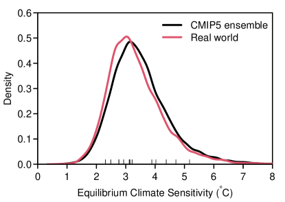
Figure 5: Equilibrium climate sensitivity. The posterior density of the equilibrium climate sensitivity for the real-world (red) and the CMIP5 ensemble (black).

Various authors have tried to constrain estimates of ECS using a variety of metrics, see Brient (2020) or Hall et al. (2019) and references therein for examples, although the credibility of some of these estimates has been questioned (Caldwell et al., 2018). Table 3 compares our estimate with that of several recent studies, including the synthesis report by Sherwood et al. (2020). Compared to the previous Bayesian hierarchical analysis by Jonko et al. (2018), our median estimate is higher, although our credible interval similar in width. This study was not targeted specifically at constraining ECS, so it is not surprising that other studies have proposed estimates that differ more strongly from the median of the models. However, both our median estimate and credible interval are very similar to those of the synthesis report by Sherwood et al. (2020).

Table 3: Estimates of Equilibrium Climate Sensitivity from the CMIP5 ensemble. Note that the IPCC interval is the “likely” 66 % interval, not a 90 % interval.

Study	Median	$5\text{\,}\mathrm{\char 37\relax}95\text{\,}\mathrm{\char 37\relax}$
IPCC		$1.5\text{\,}\mathrm{K}4.5\text{\,}\mathrm{K}$
Cox et al. Cox et al. (2018)	$2.8\text{\,}\mathrm{K}$	$1.6\text{\,}\mathrm{K}4.0\text{\,}\mathrm{K}$
Jonko et al.Jonko et al. (2018)	$2.5\text{\,}\mathrm{K}$	$1.2\text{\,}\mathrm{K}3.9\text{\,}\mathrm{K}$
Jiménez-de-la-Cuesta & Mauritsen Jiménez-de-la Cuesta and Mauritsen (2019)	$2.8\text{\,}\mathrm{K}$	$1.7\text{\,}\mathrm{K}4.1\text{\,}\mathrm{K}$
Nijsse et al. Nijsse et al. (2020)	$2.3\text{\,}\mathrm{K}$	$1.0\text{\,}\mathrm{K}4.1\text{\,}\mathrm{K}$
Sherwood et al. Sherwood et al. (2020)	$3.1\text{\,}\mathrm{K}$	$2.3\text{\,}\mathrm{K}4.7\text{\,}\mathrm{K}$
This study	$3.2\text{\,}\mathrm{K}$	$2.1\text{\,}\mathrm{K}5.1\text{\,}\mathrm{K}$

5.3 Future projections

Figure 6 shows the projections for the real-world under the RCP4.5 scenario based on the EBM fit to historical observations and accounting for shared and unique forcing bias. The projections make the usual assumption that the real-world is exchangeable with the climate model ensemble, i.e., $\kappa=1.0$. The projections are well constrained and lie entirely in the lower half of the range predicted by the CMIP5 ensemble. The mean surface temperature increase above pre-industrial conditions projected in 2100 is $2.2\text{\,}\mathrm{K}$ with 90 % credible interval $1.7\text{\,}\mathrm{K}2.9\text{\,}\mathrm{K}$. This compares with an enlarged CMIP5 ensemble (sampling new models from Equation 16) with mean $2.5\text{\,}\mathrm{K}$ with 90 % credible interval $1.6\text{\,}\mathrm{K}4.0\text{\,}\mathrm{K}$ in 2100, and an IPCC-method estimate of $2.6\text{\,}\mathrm{K}$ with 90 % credible interval $1.8\text{\,}\mathrm{K}3.4\text{\,}\mathrm{K}$.

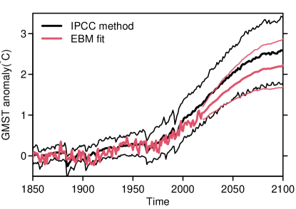
Figure 6: Global mean surface temperature anomaly projections. Posterior predictive distribution for global mean surface temperature under the RCP4.5 forcing scenario. Thick lines indicate the posterior predictive means of the CMIP5 ensemble (black) and the real-world (red). Thin lines indicate marginal 90 % credible intervals. Grey lines are the individual CMIP5 model simulations.

Table 4 compares our projections of the mean warming in the period 2081-2100 above the 1986-2005 average with other recent studies. Our estimated median warming of $1.5\text{\,}\mathrm{K}$ is $0.3\text{\,}\mathrm{K}$ lower than the other recent estimates which all agree on warming of around $1.8\text{\,}\mathrm{K}$ by the end of the century. Our credible interval is also narrower than those of the IPCC or Tokarska et al. (2020), similar to the synthesis estimate of Sherwood et al. (2020), but wider than that of Strobach and Bel (2020).

Table 4: Estimates of future warming under RCP4.5 scenario averaged over 2081–2100. Note that the IPCC and Sherwood et al. Sherwood et al. (2020) intervals are 66 % intervals, not 90 % intervals.

Study	Ensemble	Reference	Median	$5\text{\,}\mathrm{\char 37\relax}95\text{\,}\mathrm{\char 37\relax}$
IPCC	CMIP5	1986–2005	$1.8\text{\,}\mathrm{K}$	$1.1\text{\,}\mathrm{K}2.6\text{\,}\mathrm{K}$
Sherwood et al. Sherwood et al. (2020)	CMIP5	1986–2005	$1.8\text{\,}\mathrm{K}$	$1.4\text{\,}\mathrm{K}2.3\text{\,}\mathrm{K}$
Sherwood et al. Sherwood et al. (2020)	CMIP5	1986–2005	$1.8\text{\,}\mathrm{K}$	$1.7\text{\,}\mathrm{K}2.1\text{\,}\mathrm{K}$
Tokarska et al. Tokarska et al. (2020)	CMIP6	1995–2014	$1.8\text{\,}\mathrm{K}$	$1.2\text{\,}\mathrm{K}2.5\text{\,}\mathrm{K}$
This study	CMIP5	1986–2005	$1.5\text{\,}\mathrm{K}$	$1.1\text{\,}\mathrm{K}2.1\text{\,}\mathrm{K}$

Jonko et al. (2018) only made projections under the stronger RCP8.5 scenario. Our full analysis of the RCP8.5 scenario is included in the Supplementary Material. Under the RCP8.5 forcing scenario, Jonko et al. (2018) estimate a 90 % credible interval of 2.2 K–5.6 K in the year 2100 compared to the pre-industrial period (no median estimate was given). In comparison, we estimate a median warming of 4.3 K with 90 % credible interval 3.4 K–5.6 K. Given the positive skewness in the majority of estimates, our median warming is likely higher than that of Jonko et al. (2018), but our credible interval is much narrower, despite the methodological similarity. The difference in the median can be explained by our inclusion of the shared forcing discrepancy, correcting for the tendency of the EBMs to underestimate the warming in Figure 2. The difference in credible interval is likely due to the fact that Jonko et al. (2018) estimate the distribution over the models in Equation 16 from the distribution of the individual EBM parameter estimates, whereas we learn both the individual and ensemble parameters simultaneously. This results in some regularisation (shrinkage) of the individual estimates towards the consensus of the ensemble, and so a tighter distribution over the models. Since the model distribution acts as a prior for the real-world, this in turn results in a tighter distribution for the real-world.

Figure 7 shows the probabilities of meeting the targets set out in the Paris Agreement under the RCP4.5 scenario. Under the constrained projections, there is almost no probability of GMST exceeding $2.0\text{\,}\mathrm{K}$ before 2040, after which the probability rises rapidly at first then more slowly until it reaches 0.72 in 2100 in Figure 7(a). This is in striking contrast to the IPCC anomaly method which gives a probability of 0.89. The outlook for remaining below $1.5\text{\,}\mathrm{K}$ is less optimistic. The constrained projections agree with the anomaly projections that under the RCP4.5 scenario there is a probability of 0.99 that GMST will exceed $1.5\text{\,}\mathrm{K}$ above pre-industrial levels in 2100.

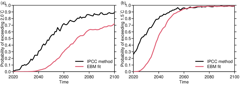
Figure 7: Probability of meeting the Paris agreement. (a) The probability of climate change below $2.0\,^{\circ}\mathrm{C}$ under the RCP4.5 forcing scenario, and (b) the probability of climate change below $1.5\,^{\circ}\mathrm{C}$ under the RCP4.5 forcing scenario.

6 Conclusions

In this study we propose a Bayesian hierarchical approach to projecting future GMST by combining outputs from multiple climate models and observations of the real-world. Our approach builds on existing methods for combining projections from multiple climate models by incorporating physically motivated representations of climate model outputs and observations. An additional innovation is the inclusion of a discrepancy in the effective forcing due to processes not captured by the simplified representation but whose effects may vary between forcing scenarios leading to biased projections. The proposed methodology not only provides point projections, but associated credible intervals and probabilities, accounting for natural variability, observation uncertainty, structural uncertainty and model inadequacy.

Compared to existing heuristic anomaly methods, observations of the real-world are integral to the projections, rather than simply an offset applied to an ensemble of models. Observations of the historical period contain limited information about the EBM representation. However, we have shown that by combining a suitable prior based on climate model outputs, there is enough information to usefully constrain projections of future climate. Although our proposed method still relies on anomalies relative to a fixed reference period, that period is now motivated by physical concerns, i.e., approximate equilibrium. Previously, the reference period would often be chosen to be as close to the present day as possible in order to limit the divergence of projections from different models. In contrast, we move the reference period as far back in time as possible and assimilate a full 170 years of annual observations rather than a single 30-year mean. Moving between reference periods for the sake of expressing results is now simply a matter of subtracting the appropriate offset between the means of the reference periods Unlike commonly used heuristic methods, the uncertainty of the projections does not change.

In forming our projections, we only used one run of each scenario from each model, when several runs of some scenarios are available from some models. By not using all available runs we are potentially throwing away valuable information. The methodology proposed here could easily be expanded to include multiple initial conditions runs without biasing our inferences towards the models with the most runs. However, the EBM representation arguably makes the inclusion of multiple runs of less value than might otherwise be the case. The EBM representation is a linear dynamic system. Therefore the response to a linear combination of inputs, i.e., known forcing and natural variability, is equal to the sum of the responses of the individual inputs. So by learning the parametric representation of the forced response, we are simultaneously learning the response to natural variability and vice-versa.

The problem of including all available models is more complicated. In order to avoid biasing our projections towards models or components that are over-represented in the CMIP5 ensemble, we chose to infer our prior for the real-world based on only a subset of the available climate models. In doing so, we risk losing valuable information contained in the excluded models. However, comparing projections from the subset against projections using the full ensemble suggests that any information loss is very limited.

Our results demonstrate that by working with physically interpretable representations and parameters, it is possible to obtain strongly constrained projections without the need to adopt performance based model weights. Having methods available that make very different assumptions is a healthy thing, since those assumptions can then be challenged and tested. The strength of the model weighting approach is that all available models can be included in the analysis. Further research is required to combine prior knowledge with dependences diagnosed from model outputs to enable the inclusion of all available models within formal statistical frameworks.

In principle, the methodology proposed here could be modified to project any future CO₂ emissions scenario. Due to the presence of shared biases in the effective forcing, we chose to learn a shared component of forcing from simulations of the future as well as historical period. This makes our parameter inference and projections specific to a particular emissions scenario and limits us to making projections of scenarios for which we have model outputs to learn from. However, if the shared discrepancy and model-specific discrepancy parameters were only learned from the historical period, the simulations could then be allowed to evolve freely following any future emissions scenario. The resulting projections would have greater uncertainty than those shown here in order to account for future changes in the shared component which is then treated as unknown. However, both the shared and specific discrepancies would require more careful specification to ensure that projections are both credible and reliable. We have shown that reliable and well constrained century scale projections are possible using simulations from only a few climate models, without having to make these additional assumptions. Further research is required to holistically quantify the effects of uncertainty about future emissions.

Appendix

Appendix A State-space representation and discretisation

Equations 1–5 can be written as

$$\frac{\operatorname{d\!}{\bm{\theta}}}{\operatorname{d\!}t} ={\bm{G}}{\bm{\theta}}(t)+{\bm{D}}{\bm{X}}(t)+{\bm{w}}(t) {\bm{w}}(t) \sim\operatorname{Normal}\left({\bm{0}},{\bm{W}}\right)$$

where

$${\bm{D}} =\begin{bmatrix}\gamma F_{C}\\ 0\\ 0\\ 0\\ \end{bmatrix} {\bm{X}}(t)=\begin{bmatrix}X_{C}(t)\end{bmatrix}$$

and

$${\bm{G}} =\begin{bmatrix}-\gamma&0&0&0\\ \frac{1}{C_{1}}&-\frac{k_{1}+k_{2}}{C_{1}}&\frac{k_{2}}{C_{1}}&0\\ 0&\frac{k_{2}}{C_{2}}&-\frac{k_{2}+\varepsilon k_{3}}{C_{2}}&\frac{\varepsilon k_{3}}{C_{2}}\\ 0&0&\frac{k_{3}}{C_{3}}&-\frac{k_{3}}{C_{3}}\\ \end{bmatrix} {\bm{W}} =\begin{bmatrix}\sigma_{F}^{2}&0&0&0\\ 0&\frac{\sigma_{T}^{2}}{C_{1}^{2}}&0&0\\ 0&0&0&0\\ 0&0&0&0\\ \end{bmatrix}.$$

Following Cummins et al. (2020), the discretised state space form of the EBM in Equations 7 and 8 is

$${\bm{F}}_{d} =\begin{bmatrix}0&1&0&0\\ 1&-k_{1}&(1-\varepsilon)k_{3}&-(1-\varepsilon)k_{3}\end{bmatrix} {\bm{V}}_{d} =\begin{bmatrix}0&0\\ 0&0\end{bmatrix}$$

where

$${\bm{G}}_{d} =e^{\bm{G}} {\bm{D}}_{d} ={\bm{G}}^{-1}({\bm{G}}_{d}-{\bm{I}}){\bm{D}} {\bm{W}}_{d} =\int_{s=0}^{1}e^{{\bm{G}}s}{\bm{W}}e^{{\bm{G}}^{\prime}s}$$

are the discretised forms of the matrices ${\bm{G}}$, ${\bm{D}}$ and ${\bm{W}}$.

Model likelihood

For parameter fitting by maximum likelihood in discrete time, the EBM likelihood factorises as

$$\Pr\left[{\bm{Y}}(1),\ldots,{\bm{Y}}(T)\mid{\bm{X}}(1),\ldots,{\bm{X}}(T),{\bm{\phi}}\right]=\prod_{t=1}^{T}\Pr\left[{\bm{Y}}(t)\mid{\bm{\mathcal{D}}}(t-1),{\bm{\phi}}\right]$$ (20)

where ${\bm{\mathcal{D}}}(t)=\left\{{\bm{Y}}(1),\ldots,{\bm{Y}}(t),{\bm{X}}(1),\ldots,{\bm{X}}(t)\right\}$ represents the data up to time $t$, and ${\bm{\phi}}=(\gamma,C_{1},C_{2},C_{3},\allowbreak k_{1},k_{2},k_{3},\varepsilon,\sigma_{F},\sigma_{T},F_{C})^{\prime}$ is the vector of EBM parameters. The likelihood can be efficiently evaluated by use of the Kalman filter.

The Kalman filter

The Kalman filter was originally conceived to provide a best estimate of the state vector ${\bm{\theta}}(t)$ given all the data up to that time. When formulated probabilistically from a Bayesian perspective, it provides prior and posterior distributions for the ${\bm{\theta}}(t)$ at each time $t$, and the prior distribution for the data ${\bm{Y}}(t)$ required to evaluate the likelihood. The familiar prediction and update steps of the Kalman filter are then:

Prediction step

The prior distribution for the state ${\bm{\theta}}$ at time $t$ given all previous data is

$$\left[{\bm{\theta}}(t)\mid{\bm{\mathcal{D}}}(t-1),{\bm{\phi}}\right]\sim\operatorname{Normal}\left[{\bm{a}}(t),{\bm{R}}(t)\right]$$ (21)

where

$${\bm{a}}(t) ={\bm{G}}_{d}{\bm{m}}(t-1)+{\bm{D}}_{d}{\bm{X}}(t) {\bm{R}}(t) ={\bm{G}}_{d}{\bm{C}}(t-1){\bm{G}}_{d}^{\prime}+{\bm{W}}_{d}$$

and ${\bm{m}}(t-1)$ and ${\bm{C}}(t-1)$ are the posterior expectation and covariance of the state ${\bm{\theta}}$ at time $t-1$.

The prior distribution for the data ${\bm{Y}}$ at time $t$ is

$$\left[{\bm{Y}}(t)\mid{\bm{\mathcal{D}}}(t-1),{\bm{\phi}}\right]\sim\operatorname{Normal}\left[{\bm{f}}(t),{\bm{Q}}(t)\right]$$ (22)

where

$${\bm{f}}(t) ={\bm{F}}_{d}{\bm{a}}(t) {\bm{Q}}(t) ={\bm{F}}_{d}{\bm{R}}(t){\bm{F}}_{d}^{\prime}+{\bm{V}}_{d}.$$

Update step

The posterior distribution of the state ${\bm{\theta}}$ at time $t$ given the data at time $t$ is then

$$\left[{\bm{\theta}}(t)\mid{\bm{\mathcal{D}}}(t),{\bm{\phi}}\right]\sim\operatorname{Normal}\left[{\bm{m}}(t),{\bm{C}}(t)\right]$$ (23)

where

$${\bm{m}}(t) ={\bm{a}}(t)+{\bm{K}}(t)\left[{\bm{Y}}(t)-{\bm{f}}(t)\right] {\bm{C}}(t) ={\bm{R}}(t)-{\bm{K}}(t){\bm{Q}}(t){\bm{K}}^{\prime}(t)$$

and ${\bm{K}}(t)={\bm{R}}(t){\bm{F}}_{d}^{\prime}{\bm{Q}}(t)^{-1}$ is the Kalman gain at time $t$.

The expected state at time $t=0$ for the abrupt 4$\times$CO₂ experiment is given by ${\bm{m}}(0)=(2F_{C},0,0,0)^{\prime}$, i.e., 4$\times$CO₂ forcing from Equation 6 applied to an initial equilibrium state. The covariance ${\bm{C}}(0)$ of the state at time $t=0$ is taken to be the stationary marginal covariance of the EBM with only stochastic forcing (Cummins et al., 2020, Appendix C).

Appendix B Projections and standardised errors

Likelihood theory tells us that the asymptotic distribution of the maximum likelihood estimator $\hat{{\bm{\phi}}}$ of the true parameters ${\bm{\phi}}$ is

$$\hat{{\bm{\phi}}}\sim\operatorname{Normal}\left[{\bm{\phi}},I({\bm{\phi}})^{-1}\right]$$

where $I({\bm{\phi}})$ is the expected information matrix. The information matrix can be computed numerically as part of the optimisation procedure used to find $\hat{\theta}$.

Therefore, given $\hat{{\bm{\phi}}}$ and equivalent CO₂ forcings $X(t)$ for the historical and RCP4.5 experiments, we can sample the full projection uncertainty due to natural variability and parameter uncertainty for each fitted model as follows:

• Sample ${\bm{\phi}}^{\star}\sim\operatorname{Normal}\left[\hat{{\bm{\phi}}},I(\hat{{\bm{\phi}}})^{-1}\right]$;

• Let ${\bm{\theta}}^{\star}(0)=\left(0,0,0,0\right)^{\prime}$, i.e., pre-industrial equilibrium;

• For $t$ in $1,\ldots,T$

  • Sample ${\bm{\theta}}^{\star}(t)$ from Equation 8, conditional on ${\bm{\theta}}^{\star}(t-1)$, $X(t)$ and ${\bm{\phi}}^{\star}$;

  • Sample ${\bm{Y}}^{\star}(t)$ from Equation 7, conditional on ${\bm{\theta}}^{\star}(t)$ and ${\bm{\phi}}^{\star}$;

By repeating the sampling procedure we can obtain as many samples ${\bm{Y}}^{\star}(1),\ldots,{\bm{Y}}^{\star}(T)$ as we wish, sampling the full extent of both the parameter uncertainty and natural variability.

The standardised prediction errors at each time $t$ are then defined as

$$\frac{Y(t)-\operatorname{E}\left[Y^{\star}(t)\right]}{\sqrt{\operatorname{Var}\left[Y^{\star}(t)\right]}}$$

where $Y(t)$ is the climate model output for the historical/RCP4.5 scenario at time $t$ and $\operatorname{E}\left[Y^{\star}(t)\right]$ and $\operatorname{Var}\left[Y^{\star}(t)\right]$ are estimated from the samples $Y^{\star}(t)$.

Appendix C Extended state space representation

The state-space representation of the extended model given by Equations 9–14 conditioned on the shared discrepancy $\nu(t)$ is given by

$${\bm{D}} =\begin{bmatrix}\gamma F_{C}&\gamma F_{V}&0\\ 0&0&0\\ 0&0&0\\ 0&0&0\\ 0&0&1\end{bmatrix} {\bm{X}}(t)=\begin{bmatrix}X_{C}(t)\\ X_{V}(t)\\ \nu(t)\end{bmatrix}$$

and

$${\bm{G}} =\begin{bmatrix}-\gamma&0&0&0&0\\ \frac{1}{C_{1}}&-\frac{k_{1}+k_{2}}{C_{1}}&\frac{k_{2}}{C_{1}}&0&\frac{1}{C_{1}}\\ 0&\frac{k_{2}}{C_{2}}&-\frac{k_{2}+\varepsilon k_{3}}{C_{2}}&\frac{\varepsilon k_{3}}{C_{2}}&0\\ 0&0&\frac{k_{3}}{C_{3}}&-\frac{k_{3}}{C_{3}}&0\\ 0&0&0&0&0\\ \end{bmatrix} {\bm{W}} =\begin{bmatrix}\sigma_{F}^{2}&0&0&0&0\\ 0&\frac{\sigma_{T}^{2}}{C_{1}^{2}}&0&0&0\\ 0&0&0&0&0\\ 0&0&0&0&0\\ 0&0&0&0&\sigma_{\delta}^{2}\\ \end{bmatrix}.$$

The discretised version is

$${\bm{F}}_{d} =\begin{bmatrix}0&1&0&0&0\\ 1&-k_{1}&(1-\varepsilon)k_{3}&-(1-\varepsilon)k_{3}&1\end{bmatrix} {\bm{V}}_{d} =\begin{bmatrix}0&0\\ 0&0\end{bmatrix}$$

and

$${\bm{G}}_{d} =e^{\bm{G}} {\bm{D}}_{d} ={\bm{G}}^{-1}({\bm{G}}_{d}-{\bm{I}}){\bm{D}} {\bm{W}}_{d} =\int_{s=0}^{1}e^{{\bm{G}}s}{\bm{W}}e^{{\bm{G}}^{\prime}s}.$$

References

- Abramowitz and Bishop [2015] Abramowitz, G., and C. H. Bishop, Climate model dependence and the ensemble dependence transformation of CMIP projections, Journal of Climate, 28(6), 2332–2348, doi:10.1175/JCLI-D-14-00364.1, 2015.
- Annan and Hargreaves [2010] Annan, J. D., and J. C. Hargreaves, Reliability of the CMIP3 ensemble, Geophysical Research Letters, 37, L02,703, doi:10.1029/2009GL041994, 2010.
- Annan and Hargreaves [2011] Annan, J. D., and J. C. Hargreaves, Understanding the CMIP3 multimodel ensemble, Journal of Climate, 24(16), 4529–4538, doi:10.1175/2011JCLI3873.1, 2011.
- Bhat et al. [2011] Bhat, K. S., M. Haran, A. Terando, and K. Keller, Climate Projections Using Bayesian Model Averaging and Space—Time Dependence, Journal of Agricultural, Biological, and Environmental Statistics, 16(4), 606–628, doi:10.1007/sl3253-011-0069-3, 2011.
- Brient [2020] Brient, F., Reducing uncertainties in climate projections with emergent constraints: Concepts, examples and prospects, Advances in Atmospheric Sciences, 37, 1–15, doi:10.1007/s00376-019-9140-8, 2020.
- Broecker [2012] Broecker, J., Probability Forecasts, in Forecast Verification: A Practicioner’s Guide in Atmostpheric Science, edited by I. T. Joliffe and D. B. Stephenson, second ed., pp. 119–140, John Wiley & Sons, Ltd., 2012.
- Buser et al. [2009] Buser, C. M., H. R. Künsch, D. Lüthi, M. Wild, and C. Schär, Bayesian multi-model projection of climate: Bias assumptions and interannual variability, Climate Dynamics, 33(6), 849–868, doi:10.1007/s00382-009-0588-6, 2009.
- Caldwell et al. [2018] Caldwell, P. M., M. D. Zelinka, and S. A. Klein, Evaluating emergent constraints on equilibrium climate sensitivity, Journal of Climate, 31(10), 3921–3942, doi:10.1175/JCLI-D-17-0631.1, 2018.
- Chandler [2013] Chandler, R. E., Exploiting strength, discounting weakness: combining information from multiple climate simulators, Philosophical Transactions of the Royal Society A: Mathematical, Physical and Engineering Sciences, 371, 20120,388, doi:10.1098/rsta.2012.0388, 2013.
- Collins [2007] Collins, M., Ensembles and probabilities: A new era in the prediction of climate change, Philosophical Transactions of the Royal Society A: Mathematical, Physical and Engineering Sciences, 365(1857), 1957–1970, doi:10.1098/rsta.2007.2068, 2007.
- Collins et al. [2013] Collins, M., et al., Long-term Climate Change: Projections, Commitments and Irreversibility, in Climate Change 2013: The Physical Science Basis, edited by T. F. Stocker, D. Qin, G.-K. Plattner, M. M. B. Tignor, S. K. Allen, J. Boschung, A. Nauels, Y. Xia, V. Bex, and P. M. Midgley, Cambridge University Press, 2013.
- Cox et al. [2018] Cox, P. M., C. Huntingford, and M. S. Williamson, Emergent constraint on equilibrium climate sensitivity from global temperature variability, Nature, 553(7688), 319–322, doi:10.1038/nature25450, 2018.
- Cummins et al. [2020] Cummins, D. P., D. B. Stephenson, and P. A. Stott, Optimal Estimation of Stochastic Energy Balance Model Parameters, Journal of Climate, 2020.
- Deser et al. [2012] Deser, C., A. S. Phillips, V. Bourdette, and H. Teng, Uncertainty in climate change projections: the role of internal variability, Climate Dynamics, 38, 527–546, doi:10.1007/s00382-010-0977-x, 2012.
- Driscoll et al. [2012] Driscoll, S., A. Bozzo, L. J. Gray, A. Robock, and G. Stenchikov, Coupled Model Intercomparison Project 5 (CMIP5) simulations of climate following volcanic eruptions, Journal of Geophysical Research Atmospheres, 117(17), doi:10.1029/2012JD017607, 2012.
- Fredriksen and Rypdal [2017] Fredriksen, H. B., and M. Rypdal, Long-range persistence in global surface temperatures explained by linear multibox energy balance models, Journal of Climate, 30(18), 7157–7168, doi:10.1175/JCLI-D-16-0877.1, 2017.
- Furrer et al. [2007] Furrer, R., S. R. Sain, D. W. Nychka, and G. A. Meehl, Multivariate Bayesian analysis of atmosphere-ocean general circulation models, Environmental and Ecological Statistics, 14(3), 249–266, doi:10.1007/s10651-007-0018-z, 2007.
- Gelman and Rubin [1992] Gelman, A., and D. B. Rubin, Inference from Iterative Simulation Using Multiple Sequences, Statistical Science, 7(4), 457–511, doi:10.1214/ss/1177011136, 1992.
- Geoffroy et al. [2013] Geoffroy, O., D. Saint-Martin, D. J. L. Olivié, A. Voldoire, G. Bellon, and S. Tytéca, Transient Climate Response in a Two-Layer Energy-Balance Model. Part I: Analytical Solution and Parameter Calibration Using CMIP5 AOGCM Experiments, Journal of Climate, 26(6), 1841–1857, doi:10.1175/JCLI-D-12-00195.1, 2013.
- Greene et al. [2006] Greene, A. M., L. Goddard, and U. Lall, Probabilistic multimodel regional temperature change projections, Journal of Climate, 19(17), 4326–4343, doi:10.1175/JCLI3864.1, 2006.
- Gregory et al. [2020] Gregory, J. M., T. Andrews, P. Ceppi, T. Mauritsen, and M. J. Webb, How accurately can the climate sensitivity to CO 2 be estimated from historical climate change?, Climate Dynamics, 54(1-2), 129–157, doi:10.1007/s00382-019-04991-y, 2020.
- Hall et al. [2019] Hall, A., P. Cox, C. Huntingford, and S. Klein, Progressing emergent constraints on future climate change, Nature Climate Change, 9(4), 269–278, doi:10.1038/s41558-019-0436-6, 2019.
- Hasselmann [1976] Hasselmann, K., Stochastic climate models Part I. Theory, Tellus, 28(6), 473–485, doi:10.3402/tellusa.v28i6.11316, 1976.
- Held et al. [2010] Held, I. M., M. Winton, K. Takahashi, T. Delworth, F. Zeng, and G. K. Vallis, Probing the fast and slow components of global warming by returning abruptly to preindustrial forcing, Journal of Climate, 23(9), 2418–2427, doi:10.1175/2009JCLI3466.1, 2010.
- Huang et al. [2020] Huang, H., D. Hammerling, B. Li, and R. Smith, Combining interdependent climate model outputs in CMIP5: A spatial Bayesian approach, 2020.
- IPCC [2018] IPCC, Global Warming of 1.5°C. An IPCC Special Report on the impacts of global warming of 1.5°C above pre-industrial levels and related global greenhouse gas emission pathways, in the context of strengthening the global response to the threat of climate change, 2018.
- Jiménez-de-la Cuesta and Mauritsen [2019] Jiménez-de-la Cuesta, D., and T. Mauritsen, Emergent constraints on Earth’s transient and equilibrium response to doubled CO2 from post-1970s global warming, Nature Geoscience, 12(11), 902–905, doi:10.1038/s41561-019-0463-y, 2019.
- Jonko et al. [2018] Jonko, A., N. M. Urban, and B. Nadiga, Towards Bayesian hierarchical inference of equilibrium climate sensitivity from a combination of CMIP5 climate models and observational data, Climatic Change, 149(2), 247–260, doi:10.1007/s10584-018-2232-0, 2018.
- Knutti et al. [2010] Knutti, R., G. Abramowitz, M. Collins, V. Eyring, P. J. Gleckler, B. Hewitson, and L. O. Mearns, Good Practice Guidance Paper on Assessing and Combining Multi Model Climate Projections, in Meeting report of the Intergovernmental Panel On Climate Change Expert Meeting on Assessing and Combining Multiple Model Climate Projections, edited by T. Stocker, Q. Dahe, G.-K. Plattner, M. Tignor, and P. Midgley, {IPCC} Working Group {I} Technical Support Unit, 2010.
- Knutti et al. [2017] Knutti, R., J. Sedláček, B. M. Sanderson, R. Lorenz, E. M. Fischer, and V. Eyring, A climate model projection weighting scheme accounting for performance and interdependence, Geophysical Research Letters, 44(4), 1909–1918, doi:10.1002/2016GL072012, 2017.
- Meinshausen et al. [2011] Meinshausen, M., et al., The RCP greenhouse gas concentrations and their extensions from 1765 to 2300, Climatic Change, 109(1), 213–241, doi:10.1007/s10584-011-0156-z, 2011.
- Min and Hense [2006] Min, S. K., and A. Hense, A Bayesian approach to climate model evaluation and multi-model averaging with an application to global mean surface temperatures from IPCC AR4 coupled climate models, Geophysical Research Letters, 33(8), L08,708, doi:10.1029/2006GL025779, 2006.
- Morice et al. [2012] Morice, C. P., J. J. Kennedy, N. A. Rayner, and P. D. Jones, Quantifying uncertainties in global and regional temperature change using an ensemble of observational estimates: The HadCRUT4 data set, Journal of Geophysical Research Atmospheres, 117(8), 1–22, doi:10.1029/2011JD017187, 2012.
- Moss et al. [2010] Moss, R. H., et al., The next generation of scenarios for climate change research and assessment, Nature, 463(7282), 747–756, doi:10.1038/nature08823, 2010.
- Nijsse et al. [2020] Nijsse, F., P. Cox, and M. Williamson, An emergent constraint on Transient Climate Response from simulated historical warming in CMIP6 models, Earth System Dynamics Discussions, pp. 1–14, doi:10.5194/esd-2019-86, 2020.
- Palmer et al. [2006] Palmer, T., R. Buizza, R. Hagedorn, A. Lawrence, M. Leutbecher, and L. A. Smith, Ensemble prediction: a pedagogical perspective, ECMWF Newsletter, 106, 10–17, doi:10.21957/ab129056ew, 2006.
- Räisänen and Palmer [2001] Räisänen, J., and T. N. Palmer, A probability and decision-model analysis of a multimodel ensemble of climate change simulations, Journal of Climate, 14(15), 3212–3226, doi:10.1175/1520-0442(2001)014¡3212:APADMA¿2.0.CO;2, 2001.
- Rougier et al. [2013] Rougier, J. C., M. Goldstein, and L. House, Second-Order Exchangeability Analysis for Multimodel Ensembles, Journal of the American Statistical Association, 108(503), 852–863, doi:10.1080/01621459.2013.802963, 2013.
- Sanderson et al. [2017] Sanderson, B. M., M. Wehner, and R. Knutti, Skill and independence weighting for multi-model assessments, Geoscientific Model Development, 10(6), 2379–2395, doi:10.5194/gmd-10-2379-2017, 2017.
- Sansom et al. [2013] Sansom, P. G., D. B. Stephenson, C. A. T. Ferro, G. Zappa, and L. C. Shaffrey, Simple uncertainty frameworks for selecting weighting schemes and interpreting multimodel ensemble climate change experiments, Journal of Climate, 26, 4017–4037, doi:10.1175/JCLI-D-12-00462.1, 2013.
- Sansom et al. [2020] Sansom, P. G., D. B. Stephenson, and T. J. Bracegirdle, On constraining projections of future climate using observations and simulations from multiple climate models, Journal of the American Statistical Association, p. In review, 2020.
- Sato et al. [1993] Sato, M., J. E. Hansen, M. P. McCormick, and J. B. Pollack, Stratospheric Aerosol Optical Depths, 1850-1990, 98, 22,987–22,994, doi:10.1029/93JD02553, 1993.
- Sherwood et al. [2020] Sherwood, S. C., et al., An assessment of Earth’s climate sensitivity using multiple lines of evidence, 0–2 pp., doi:10.1029/2019rg000678, 2020.
- Shiogama et al. [2011] Shiogama, H., S. Emori, N. Hanasaki, M. Abe, Y. Masutomi, K. Takahashi, and T. Nozawa, Observational constraints indicate risk of drying in the Amazon basin., Nature communications, 2, 253, doi:10.1038/ncomms1252, 2011.
- Smith [2002] Smith, L. A., What might we learn from climate forecasts?, Proceedings of the National Academy of Sciences of the United States of America, 99(SUPPL. 1), 2487–2492, doi:10.1073/pnas.012580599, 2002.
- Smith et al. [2009] Smith, R. L., C. Tebaldi, D. W. Nychka, and L. O. Mearns, Bayesian Modeling of Uncertainty in Ensembles of Climate Models, Journal of the American Statistical Association, 104(485), 97–116, doi:10.1198/jasa.2009.0007, 2009.
- Stainforth et al. [2007] Stainforth, D. A., M. R. Allen, E. R. Tredger, and L. A. Smith, Confidence, uncertainty and decision-support relevance in climate predictions, Philosophical Transactions of the Royal Society A, 365, 2145–2161, doi:10.1098/rsta.2007.2074, 2007.
- Stephenson et al. [2012] Stephenson, D. B., M. Collins, J. C. Rougier, and R. E. Chandler, Statistical problems in the probabilistic prediction of climate change, Environmetrics, 23(5), 364–372, doi:10.1002/env.2153, 2012.
- Strobach and Bel [2020] Strobach, E., and G. Bel, Learning algorithms allow for improved reliability and accuracy of global mean surface temperature projections, Nature Communications, 11(1), 1–7, doi:10.1038/s41467-020-14342-9, 2020.
- Sutton et al. [2015] Sutton, R., E. Suckling, and E. Hawkins, What does global mean temperature tell us about local climate?, Philosophical Transactions of the Royal Society A: Mathematical, Physical and Engineering Sciences, 373(2054), doi:10.1098/rsta.2014.0426, 2015.
- Taylor et al. [2012] Taylor, K. E., R. J. Stouffer, and G. A. Meehl, An overview of CMIP5 and the experiment design, Bulletin of the American Meteorological Society, 93(4), 485–498, doi:10.1175/BAMS-D-11-00094.1, 2012.
- Tebaldi and Knutti [2007] Tebaldi, C., and R. Knutti, The use of the multi-model ensemble in probabilistic climate projections, Philosophical Transactions of the Royal Society A: Mathematical, Physical and Engineering Sciences, 365(1857), 2053–2075, doi:10.1098/rsta.2007.2076, 2007.
- Tebaldi and Sansó [2009] Tebaldi, C., and B. Sansó, Joint projections of temperature and precipitation change from multiple climate models: A hierarchical Bayesian approach, Journal of the Royal Statistical Society: Series A (Statistics in Society), 172(1), 83–106, doi:10.1111/j.1467-985X.2008.00545.x, 2009.
- Tebaldi et al. [2005] Tebaldi, C., R. L. Smith, D. W. Nychka, and L. O. Mearns, Quantifying uncertainty in projections of regional climate change: A Bayesian approach to the analysis of multimodel ensembles, Journal of Climate, 18(10), 1524–1540, doi:10.1175/JCLI3363.1, 2005.
- Tokarska et al. [2020] Tokarska, K. B., M. B. Stolpe, S. Sippel, E. M. Fischer, C. J. Smith, F. Lehner, and R. Knutti, Past warming trend constrains future warming in CMIP6 models, Science Advances, 6(12), 1–14, doi:10.1126/sciadv.aaz9549, 2020.
- Vihola [2012] Vihola, M., Robust adaptive Metropolis algorithm with coerced acceptance rate, Statistics and Computing, 22(5), 997–1008, doi:10.1007/s11222-011-9269-5, 2012.
- Watterson and Whetton [2011] Watterson, I. G., and P. H. Whetton, Distributions of decadal means of temperature and precipitation change under global warming, Journal of Geophysical Research: Atmospheres, 116(7), 1–13, doi:10.1029/2010JD014502, 2011.
- Weigel et al. [2010] Weigel, A. P., R. Knutti, M. A. Liniger, and C. Appenzeller, Risks of model weighting in multimodel climate projections, Journal of Climate, 23(15), 4175–4191, doi:10.1175/2010JCLI3594.1, 2010.