Weak Convergence for Variational Inequalities with Inertial-Type Method

Abstract

Weak convergence of inertial iterative method for solving variational inequalities is the focus of this paper. The cost function is assumed to be non-Lipschitz and monotone. We propose a projection-type method with inertial terms and give weak convergence analysis under appropriate conditions. Some test results are performed and compared with relevant methods in the literature to show the efficiency and advantages given by our proposed methods.

1 Introduction

Suppose $C$ is a nonempty, closed and convex subset of a real Hilbert space $H$ and $F:C\rightarrow H$ a continuous mapping. The variational inequality problem (for short, VI($F,C$)) is defined as: find $x\in C$ such that

$$\langle F(x),y-x\rangle\geq 0,\quad\forall y\in C.$$ (1)

We shall denote by SOL the solution set of VI($F,C$) in (1). Various applications of variational inequality can be found in [7, 8, 23, 24, 25, 33, 34, 35, 43].

Projection-type method for solving VI($F,C$) (1) have been considered severally in the literature (see, for example, [16, 17, 18, 22, 29, 40, 41, 42, 45, 48, 56]). Several other related methods to extragradient method and (5) for solving VI($F,C$) (1) in real Hilbert spaces when $F$ is monotone and $L$-Lipschitz-continuous mapping have been studied in the literature (see, for example, [16, 17, 18, 22, 29, 36, 40, 41, 42, 45, 56]). Some of these methods involve computing projection onto the feasible set $C$ twice per iteration and this can affect the efficiency of the methods.

In [19], Censor et al. introduced the subgradient extragradient method: $x_{1}\in H$,

$$\left\{\begin{array}[]{llll}&y_{n}=P_{C}(x_{n}-\lambda F(x_{n})),\\ &T_{n}:=\{w\in H:\langle x_{n}-\lambda F(x_{n})-y_{n},w-y_{n}\rangle\leq 0\},\\ &x_{n+1}=P_{T_{n}}(x_{n}-\lambda F(y_{n}))\end{array}\right.$$ (5)

and gave weak convergence result when $F$ is monotone and $L$-Lipschitz-continuous mapping where $\lambda\in(0,\frac{1}{L})$.

In order to accelerate the convergence of subgradient extragradient method (5) and using the idea of in [2, 3, 4, 5, 6, 10, 12, 13, 20, 37, 38, 46, 47], Thong and Hieu [55] introduced the following inertial subgradient extragradient method: $x_{0},x_{1}\in H$,

$$\left\{\begin{array}[]{llll}&w_{n}=x_{n}+\alpha_{n}(x_{n}-x_{n-1}),\\ &y_{n}=P_{C}(w_{n}-\lambda F(w_{n})),\\ &T_{n}:=\{w\in H:\langle w_{n}-\lambda F(w_{n})-y_{n},w-y_{n}\rangle\leq 0\},\\ &x_{n+1}=P_{T_{n}}(w_{n}-\lambda F(y_{n}))\end{array}\right.$$ (10)

and proved that $\{x_{n}\}$ generated by (10) converges weakly to a solution of VI($F,C$) (1) when $F$ is monotone and $L$-Lipschitz-continuous mapping $F$ where $0<\lambda L\leq\frac{\frac{1}{2}-2\alpha-\frac{1}{2}\alpha^{2}-\delta}{\frac{1}{2}-\alpha+\frac{1}{2}\alpha^{2}}$ for some $0<\delta<\frac{1}{2}-2\alpha-\frac{1}{2}\alpha^{2}$ and $\{\alpha_{n}\}$ is a non-decreasing sequence with $0\leq\alpha_{n}\leq\alpha<\sqrt{5}-2$.

The step-sizes in above methods (5) and (10) are bounded by the inverse of the Lipschitz constant and this is quite inefficient, since in most applications a global Lipschitz constant (if it indeed exists at all) of $F$ cannot be accurately estimated, and is usually overestimated. This leads to too small step-sizes, which, of course, is not practical. Therefore, algorithms (5) and (10) are not applicable in most cases of interest. This can be overcome by using an Armijo type line search procedure (see [33, 43, 53]).

We provide a simple example of a variational inequality problem where the method (5) proposed in [19] and method (10) proposed in [55] cannot be applied.

Example 1.1.

Suppose $F:[0,\infty)\rightarrow\mathbb{R}$ is defined by $F(x):=e^{x},\leavevmode\nobreak\ x\in[0,\infty)$. It is easy to see that $F$ is not Lipschitz continuous on $[0,\infty)$. By the mean value theorem, one has for an arbitrary $r>0$,

$$|F(x)-F(y)|\leq e^{r}|x-y|$$

with $|x|,|y|\leq r$. Hence, $F$ is uniformly continuous on bounded subsets of $C:=[0,\infty)$. Consequently, one can easily see that $F$ is monotone on $[0,\infty)$ since

$$\langle F(x)-F(y),x-y\rangle=(F(x)-F(y))(x-y)\geq 0,\leavevmode\nobreak\ \leavevmode\nobreak\ \forall x,y\in[0,\infty).$$

Finally, SOL of VI$(F,C)$ is nonempty since $0\in\text{SOL}$.

Motivated by Example 1.1, it would be of interest to propose an iterative method for solving VI($F,C$) (1) for which the underline cost function $F$ is uniformly continuous on bounded subsets of $C$ but not Lipschitz continuous on $C$.

Our interest in this paper is to obtain weak convergence results using inertial projection-type algorithm for VI($F,C$) (1) when the underline operator $F$ is monotone and uniformly continuous. We do not assume the cost function to be Lipschitz continuous as assumed in [18, 19, 22, 40, 41, 55]. Our proposed method is much more practical and outperforms the methods (5) and (10) numerically.

We organize the paper as follows: Basic definitions and results are given in Section 2 and the proposed method is introduced in Section 3. We give weak convergence analysis of the proposed method in Section 4 and give some numerical comparisons of our method with methods (5) and (10) in Section 5. Finally, we some concluding remarks in Section 6.

2 Preliminaries

Suppose we take $H$ as a real Hilbert space and $X\subseteq H$ be a nonempty subset.

Definition 2.1.

A mapping $F:X\to H$ is called

• monotone on $X$ if $\langle F(x)-F(y),x-y\rangle\geq 0$ for all $x,y\in X$;

• Lipschitz continuous on $X$ if there exists a constant $L>0$ such that

  $$\|F(x)-F(y)\|\leq L\|x-y\|,\ \forall x,y\in X.$$

• sequentially weakly continuous if for each sequence $\{x_{n}\}$ we have: $\{x_{n}\}$ converges weakly to $x$ implies $\{F(x_{n})\}$ converges weakly to $F(x)$.

Given any point $u\in H$, there exists a unique point $P_{C}u\in C$ (see, e.g., [9]) such that

$$\|u-P_{C}u\|\leq\|u-y\|,\leavevmode\nobreak\ \forall y\in C.$$

This $P_{C}$ is called the metric projection of $H$ onto $C$. It is known that $P_{C}$ is a nonexpansive mapping of $H$ onto $C$ and satisfies

$$\langle x-y,P_{C}x-P_{C}y\rangle\geq\|P_{C}x-P_{C}y\|^{2},\leavevmode\nobreak\ \leavevmode\nobreak\ \forall x,y\in H.$$ (11)

In particular, we get from (11) that

$$\langle x-y,x-P_{C}y\rangle\geq\|x-P_{C}y\|^{2},\leavevmode\nobreak\ \leavevmode\nobreak\ \forall x\in C,y\in H.$$ (12)

Another property of $P_{C}x$ is :

$$P_{C}x\in C\quad\text{and}\quad\langle x-P_{C}x,P_{C}x-y\rangle\geq 0,\leavevmode\nobreak\ \forall y\in C.$$ (13)

More details on $P_{C}$ can be found, for example, in Section 3 of [26].

The following results are needed in the next section.

Lemma 2.2.

The following statements hold in $H$:

• $\|x+y\|^{2}=\|x\|^{2}+2\langle x,y\rangle+\|y\|^{2}$ for all $x,y\in H$;

• $2\langle x-y,x-z\rangle=\|x-y\|^{2}+\|x-z\|^{2}-\|y-z\|^{2}$ for all $x,y,z\in H$;

• $\|\alpha x+(1-\alpha)y\|^{2}=\alpha\|x\|^{2}+(1-\alpha)\|y\|^{2}-\alpha(1-\alpha)\|x-y\|^{2}$ for all $x,y\in H$ and $\alpha\in\mathbb{R}$.

Lemma 2.3.

(see [1, Lem. 3]) Let $\{\psi_{n}\}$, $\{\delta_{n}\}$ and $\{\alpha_{n}\}$ be the sequences in $[0,+\infty)$ such that $\psi_{n+1}\leq\psi_{n}+\alpha_{n}(\psi_{n}-\psi_{n-1})+\delta_{n}$ for all $n\geq 1$, $\sum_{n=1}^{\infty}\delta_{n}<+\infty$ and there exists a real number $\alpha$ with $0\leq\alpha_{n}\leq\alpha<1$ for all $n\geq 1$. Then the following hold:
$(i)\leavevmode\nobreak\ \leavevmode\nobreak\ \sum_{n\geq 1}[\psi_{n}-\psi_{n-1}]_{+}<+\infty$, where $[t]_{+}=\max\{t,0\}$;
(ii) there exists $\psi^{*}\in[0,+\infty)$ such that $\lim_{n\rightarrow+\infty}\psi_{n}=\psi^{*}$.

Lemma 2.4.

(see [9, Lem. 2.39]) Let $C$ be a nonempty set of $H$ and $\{x_{n}\}$ be a sequence in $H$ such that the following two conditions hold:
(i) for any $x\in C$, $\lim_{n\rightarrow\infty}\|x_{n}-x\|$ exists;
(ii) every sequential weak cluster point of $\{x_{n}\}$ is in $C$.
Then $\{x_{n}\}$ converges weakly to a point in $C$.

Lemma 2.5.

([28]) Let $C$ be a nonempty closed and convex subset of $H$. Let $h$ be a real-valued function on $H$ and define $K:=\{x:h(x)\leq 0\}$. If $K$ is nonempty and $h$ is Lipschitz continuous on $C$ with modulus $\theta>0$, then

$${\rm dist}(x,K)\geq\theta^{-1}\max\{h(x),0\},\leavevmode\nobreak\ \forall x\in C,$$

where ${\rm dist}(x,K)$ denotes the distance function from $x$ to $K$.

Lemma 2.6.

Let $C$ be a nonempty closed and convex subset of $H$, $y:=P_{C}(x)$ and $x^{*}\in C$. Then

$$\|y-x^{*}\|^{2}\leq\|x-x^{*}\|^{2}-\|x-y\|^{2}.$$ (14)

Lemma 2.7.

([31, Prop. 2.11], [30, Prop. 4]) Let $H_{1}$ and $H_{2}$ be two real Hilbert spaces. Suppose $F:H_{1}\rightarrow H_{2}$ is uniformly continuous on bounded subsets of $H_{1}$ and $M$ is a bounded subset of $H_{1}$. Then $F(M)$ is bounded.

Lemma 2.8.

([54, Lem. 7.1.7]) Let $C$ be a nonempty, closed, and convex subset of $H$. Let $F:C\rightarrow H$ be a continuous, monotone mapping and $z\in C$. Then

$$z\in{\rm SOL}\Longleftrightarrow\langle F(x),x-z\rangle\geq 0\quad\text{for all }x\in C.$$

3 Proposed Method

We give some assumptions on the feasible set $C$, the cost function $F$ and the iterative parameter $\{\alpha_{n}\}$ below.

Assumption 3.1.

Suppose that the following hold:

• The feasible set $C$ is a nonempty closed affine subset of the real Hilbert space $H$.

• $F:C\to H$ is monotone and uniformly continuous on bounded subsets of $H$.

• The solution set SOL of VI$(F,C)$ is nonempty.

Assumption 3.2.

Suppose the real sequence $\{\alpha_{n}\}$ satisfy the following condition:

• $\{\alpha_{n}\}\subset(0,1)$ with $0\leq\alpha_{n}\leq\alpha_{n+1}\leq\alpha<\frac{1}{3}$ for all $n$.

Suppose we define

$$r(x):=x-P_{C}(x-F(x))$$

as the residual equation. Then if $y=x-F(x)$ in (12), we obtain

$$\langle F(x),r(x)\rangle\geq\|r(x)\|^{2},\leavevmode\nobreak\ \forall x\in C.$$ (15)

We next give our proposed inertial projection-type method.

Algorithm 1 Inertial Projection Method

1:Choose sequence $\{\alpha_{n}\}$ and $\sigma\in(0,1)$ such that the conditions from Assumption 3.2 hold, and take $\gamma\in(0,1)$. Let $x_{0}=x_{1}\in H$ be a given starting point. Set $n:=1$.

2:Set

$$w_{n}:=x_{n}+\alpha_{n}(x_{n}-x_{n-1}).$$

Compute $z_{n}:=P_{C}(w_{n}-F(w_{n}))$. If $r(w_{n})=w_{n}-z_{n}=0$: STOP.

3:Compute $y_{n}=w_{n}-\gamma^{m_{n}}r(w_{n})$, where $m_{n}$ is the smallest nonnegative integer satisfying

$$\langle F(y_{n}),r(w_{n})\rangle\geq\frac{\sigma}{2}\|r(w_{n})\|^{2}.$$ (16)

Set $\eta_{n}:=\gamma^{m_{n}}$.

4:Compute

$$x_{n+1}=P_{C_{n}}(w_{n}),$$ (17)

where $C_{n}=\{x:h_{n}(x)\leq 0\}$ and

$$h_{n}(x):=\langle F(y_{n}),x-y_{n}\rangle.$$ (18)

5:Set $n\leftarrow n+1$ and goto 2.

If $r(w_{n})=0$, then $w_{n}$ is a solution of VI($F,C$) (1). In the analysis we assume that $r(w_{n})\neq 0$ for infinitely many iterations, so that Algorithm 1 generates an infinite sequence satisfying $r(w_{n})\neq 0$ for all $n\in\mathbb{N}$.

Remark 3.3.

(a) Our proposed Algorithm 1 requires, at each iteration, only one projection onto the feasible set $C$ and another projection onto the half-space $C_{n}$ (which has a closed form solution, [15]) and this is numerically less expensive than the twice computation of projection onto $C$ per iteration in extragradient method [36].

(b) As we have mentioned before, Algorithm 1 is much more applicable than (5) and (10) because the Lipschtz constant of the cost function $F$ is not needed during implementations. $\Diamond$

Lemma 3.4.

Let the function $h_{n}$ be defined by (18). Then

$$h_{n}(w_{n})\geq\frac{\sigma\eta_{n}}{2}\|w_{n}-z_{n}\|^{2}.$$

In particular, if $w_{n}\neq z_{n}$, then $h_{n}(w_{n})>0$. If $x^{*}\in\text{SOL}$, then $h_{n}(x^{*})\leq 0$.

Proof.

Since $y_{n}=w_{n}-\eta_{n}(w_{n}-z_{n})$, using (16) we have

$$h_{n}(w_{n}) =\langle F(y_{n}),w_{n}-y_{n}\rangle$$

$$=\eta_{n}\langle F(y_{n}),w_{n}-z_{n}\rangle\geq\eta_{n}\frac{\sigma}{2}\|w_{n}-z_{n}\|^{2}\geq 0.$$

If $w_{n}\neq z_{n}$, then $h_{n}(w_{n})>0$. Furthermore, suppose $x^{*}\in\text{SOL}$. Then by Lemma 2.8 we have $\langle F(x),x-x^{*}\rangle\geq 0\quad\text{for all }x\in C.$ In particular, $\langle F(y_{n}),y_{n}-x^{*}\rangle\geq 0$ and hence $h_{n}(x^{*})\leq 0.$ ∎

4 Convergence Analysis

Let us give weak convergence analysis of our proposed Algorithm 1 in this section.

Lemma 4.1.

Let $\{x_{n}\}$ be generated by Algorithm 1. Then under Assumptions 3.1 and 3.2, we have that
(i)  $\{x_{n}\}$ is bounded, and
(ii)  $\lim_{n\rightarrow\infty}\|x_{n+1}-w_{n}\|=0$.

Proof.

Let $x^{*}\in\text{SOL}$. By Lemma 2.6 we get (since $x^{*}\in C_{n}$) that

$$\|x_{n+1}-x^{*}\|^{2} = \|P_{C_{n}}(w_{n})-x^{*}\|^{2}\leq\|w_{n}-x^{*}\|^{2}-\|x_{n+1}-w_{n}\|^{2}$$

$$= \|w_{n}-x^{*}\|^{2}-{\rm dist}^{2}(w_{n},C_{n}).$$

Now, using Lemma 2.2 (c), we have

$$\|w_{n}-x^{*}\|^{2} = \|(1+\alpha_{n})(x_{n}-x^{*})-\alpha_{n}(x_{n-1}-x^{*})\|^{2}$$ (20)

$$= (1+\alpha_{n})\|x_{n}-x^{*}\|^{2}-\alpha_{n}\|x_{n-1}-x^{*}\|$$

$$+\alpha_{n}(1+\alpha_{n})\|x_{n}-x_{n-1}\|^{2}.$$

Also,

$$\|x_{n+1}-w_{n}\|^{2} = \|x_{n+1}-(x_{n}+\alpha_{n}(x_{n}-x_{n-1}))\|^{2}$$ (21)

$$= \|x_{n+1}-x_{n}\|^{2}+\alpha^{2}_{k}\|x_{n}-x_{n-1}\|^{2}-2\alpha_{n}\langle x_{n+1}-x_{n},x_{n}-x_{n-1}\rangle$$

$$\geq \|x_{n+1}-x_{n}\|^{2}+\alpha^{2}_{k}\|x_{n}-x_{n-1}\|^{2}-2\alpha_{n}\|x_{n+1}-x_{n}\|\|x_{n}-x_{n-1}\|$$

$$\geq \|x_{n+1}-x_{n}\|^{2}+\alpha^{2}_{k}\|x_{n}-x_{n-1}\|^{2}-\alpha_{n}\|x_{n+1}-x_{n}\|^{2}$$

$$-\alpha_{n}\|x_{n}-x_{n-1}\|^{2}$$

$$= (1-\alpha_{n})\|x_{n+1}-x_{n}\|^{2}+(\alpha_{n}^{2}-\alpha_{n})\|x_{n}-x_{n-1}\|^{2}.$$

Combining (4), (20) and (21), we get

$$\|x_{n+1}-x^{*}\|^{2} \leq (1+\alpha_{n})\|x_{n}-x^{*}\|^{2}-\alpha_{n}\|x_{n-1}-x^{*}\|^{2}$$ (22)

$$+\alpha_{n}(1+\alpha_{n})\|x_{n}-x_{n-1}\|^{2}-(1-\alpha_{n})\|x_{n+1}-x_{n}\|^{2}$$

$$-(\alpha_{n}^{2}-\alpha_{n})\|x_{n}-x_{n-1}\|^{2}$$

$$= (1+\alpha_{n})\|x_{n}-x^{*}\|^{2}-\alpha_{n}\|x_{n-1}-x^{*}\|^{2}$$

$$-(1-\alpha_{n})\|x_{n+1}-x_{n}\|^{2}+(\alpha_{n}(1+\alpha_{n})-(\alpha_{n}^{2}-\alpha_{n}))\|x_{n}-x_{n-1}\|^{2}$$

$$= (1+\alpha_{n})\|x_{n}-x^{*}\|^{2}-\alpha_{n}\|x_{n-1}-x^{*}\|^{2}$$

$$-(1-\alpha_{n})\|x_{n+1}-x_{n}\|^{2}+2\alpha_{n}\|x_{n}-x_{n-1}\|^{2}.$$

Using the fact that $\alpha_{n}\leq\alpha_{n+1}$, we obtain from (22) that

$$\|x_{n+1}-x^{*}\|^{2} \leq (1+\alpha_{n+1})\|x_{n}-x^{*}\|^{2}-\alpha_{n}\|x_{n-1}-x^{*}\|^{2}$$ (23)

$$-(1-\alpha_{n})\|x_{n+1}-x_{n}\|^{2}+2\alpha_{n}\|x_{n}-x_{n-1}\|^{2}.$$

By (23), we get

$$\|x_{n+1}-x^{*}\|^{2}-\alpha_{n+1}\|x_{n}-x^{*}\|^{2}+2\alpha_{n+1}\|x_{n+1}-x_{n}\|^{2}\leq\|x_{n}-x^{*}\|^{2}-\alpha_{n}\|x_{n-1}-x^{*}\|^{2}$$

$$+2\alpha_{n}\|x_{n}-x_{n-1}\|^{2}+2\alpha_{n+1}\|x_{n+1}-x_{n}\|^{2}-(1-\alpha_{n})\|x_{n+1}-x_{n}\|^{2}$$

$$= \|x_{n}-x^{*}\|^{2}-\alpha_{n}\|x_{n-1}-x^{*}\|^{2}+2\alpha_{n}\|x_{n}-x_{n-1}\|^{2}+(2\alpha_{n+1}-1+\alpha_{n})\|x_{n+1}-x_{n}\|^{2}.$$

Therefore,

$$\|x_{n+1}-x^{*}\|^{2} \leq \|x_{n}-x^{*}\|^{2}-\alpha_{n}\|x_{n-1}-x^{*}\|^{2}+2\alpha_{n}\|x_{n}-x_{n-1}\|^{2}$$ (24)

$$+(2\alpha_{n+1}-1+\alpha_{n})\|x_{n+1}-x_{n}\|^{2}.$$

Let us define

$$\Gamma_{n}:=\|x_{n}-x^{*}\|^{2}-\alpha_{n}\|x_{n-1}-x^{*}\|^{2}+2\alpha_{n}\|x_{n}-x_{n-1}\|^{2}.$$

Then we have from (24) that

$$\Gamma_{n+1}-\Gamma_{n}\leq(2\alpha_{n+1}-1+\alpha_{n})\|x_{n+1}-x_{n}\|^{2}.$$ (25)

Since $0\leq\alpha_{n}\leq\alpha_{n+1}\leq\alpha<\frac{1}{3}$, we get $-2\alpha_{n+1}\geq-2\alpha$ and $-\alpha_{n}\geq-\alpha$. This implies that $-(2\alpha_{n+1}-1+\alpha_{n})=-2\alpha_{n+1}+1-\alpha_{n}\geq-2\alpha+1-\alpha\geq 1-3\alpha>0$ since $\alpha<\frac{1}{3}$. Now, let us define $\sigma:=1-3\alpha$. Then

$$2\alpha_{n+1}-1+\alpha_{n}\leq-\sigma.$$ (26)

Putting (26) into (25), we have

$$\Gamma_{n+1}-\Gamma_{n}\leq-\sigma\|x_{n+1}-x_{n}\|^{2}.$$ (27)

From (27), we see that $\{\Gamma_{n}\}$ is monotone nonincreasing. Furthermore,

$$\Gamma_{n} = \|x_{n}-x^{*}\|^{2}-\alpha_{n}\|x_{n-1}-x^{*}\|^{2}+2\alpha_{n}\|x_{n}-x_{n-1}\|^{2}$$ (28)

$$\geq \|x_{n}-x^{*}\|^{2}-\alpha_{n}\|x_{n-1}-x^{*}\|^{2}.$$

So,

$$\|x_{n}-x^{*}\|^{2} \leq \alpha_{n}\|x_{n-1}-x^{*}\|^{2}+\Gamma_{n}$$ (29)

$$\leq \alpha\|x_{n-1}-x^{*}\|^{2}+\Gamma_{1}$$

$$\vdots$$

$$\leq \alpha^{k}\|x_{0}-x^{*}\|^{2}+(1+\alpha+\alpha^{2}+\ldots+\alpha^{k-1})\Gamma_{1}$$

$$= \alpha^{k}\|x_{0}-x^{*}\|^{2}+\frac{\Gamma_{1}}{1-\alpha}.$$

From (29), we can infer that $\{x_{n}\}$ is bounded. Using the definition of $\Gamma_{n}$, we have

$$\Gamma_{n+1} = \|x_{n+1}-x^{*}\|^{2}-\alpha_{n+1}\|x_{n}-x^{*}\|^{2}+2\alpha_{n+1}\|x_{n+1}-x_{n}\|^{2}$$ (30)

$$\geq -\alpha_{n+1}\|x_{n}-x^{*}\|^{2}.$$

Using (29) in (30), we get

$$-\Gamma_{n+1} \leq -\alpha_{n+1}\|x_{n}-x^{*}\|^{2}\leq\alpha\|x_{n}-x^{*}\|^{2}$$ (31)

$$\leq \alpha^{k+1}\|x_{0}-x^{*}\|^{2}+\frac{\alpha\Gamma_{1}}{1-\alpha}.$$

From (27), we get

$$\sigma\|x_{n+1}-x_{n}\|^{2}\leq\Gamma_{n}-\Gamma_{n+1}$$

and so

$$\sigma\sum_{j=1}^{n}\|x_{j+1}-x_{j}\|^{2} \leq \Gamma_{1}-\Gamma_{n+1}$$

$$\leq \Gamma_{1}+\alpha^{n+1}\|x_{0}-x^{*}\|^{2}+\frac{\alpha\Gamma_{1}}{1-\alpha}$$

$$\leq \alpha^{n+1}\|x_{0}-x^{*}\|^{2}+\frac{\Gamma_{1}}{1-\alpha}$$

$$\leq \|x_{0}-x^{*}\|^{2}+\frac{\Gamma_{1}}{1-\alpha}.$$

Therefore, since $x_{0}=x_{1}$, we get

$$\sum_{k=1}^{\infty}\|x_{n+1}-x_{n}\|^{2} \leq \frac{1}{\sigma}\Big{(}\|x_{0}-x^{*}\|^{2}+\frac{\Gamma_{1}}{1-\alpha}\Big{)}$$

$$= \frac{1}{\sigma}\|x_{0}-x^{*}\|^{2}+\frac{1-\alpha_{1}}{1-\alpha}\|x_{0}-x^{*}\|^{2}$$

$$= \Big{(}\frac{1}{1-3\alpha}+\frac{1-\alpha_{1}}{1-\alpha}\Big{)}\|x_{0}-x^{*}\|^{2}<\infty.$$

Observe that

$$\|x_{n+1}-w_{n}\| = \|x_{n+1}-x_{n}-\alpha_{n}(x_{n}-x_{n-1})\|$$ (32)

$$\leq \|x_{n+1}-x_{n}\|+\alpha_{n}\|x_{n}-x_{n-1}\|$$

$$\leq \|x_{n+1}-x_{n}\|+\alpha\|x_{n}-x_{n-1}\|.$$

Using (32), we obtain

$$\lim_{n\rightarrow\infty}\|x_{n+1}-w_{n}\|=0.$$ (33)

∎

Lemma 4.2.

Let $\{x_{n}\}$ generated by Algorithm 1 above and Assumptions 3.1 and 3.2 hold. Then

• $\displaystyle\lim_{n\rightarrow\infty}\eta_{n}\|w_{n}-z_{n}\|^{2}=0$;

• $\displaystyle\lim_{n\rightarrow\infty}\|w_{n}-z_{n}\|=0.$

Proof.

Let $x^{*}\in\text{SOL}$. Since $F$ is uniformly continuous on bounded subsets of $X$, then $\{F(x_{n})\},\{z_{n}\},\{w_{n}\}$ and $\{F(y_{n})\}$ are bounded. In particular, there exists $M>0$ such that $\|F(y_{n})\|\leq M$ for all $n\in\mathbb{N}$. Combining Lemma 2.5 and Lemma 3.4, we get

$$\|x_{n+1}-x^{*}\|^{2} = \|P_{C_{n}}(w_{n})-x^{*}\|^{2}\leq\|w_{n}-x^{*}\|^{2}-\|x_{n+1}-w_{n}\|^{2}$$ (34)

$$= \|w_{n}-x^{*}\|^{2}-{\rm dist}^{2}(w_{n},C_{n})$$

$$\leq \|w_{n}-x^{*}\|^{2}-\Big{(}\frac{1}{M}h_{n}(w_{n})\Big{)}^{2}$$

$$\leq \|w_{n}-x^{*}\|^{2}-\Big{(}\frac{1}{2M}\sigma\eta_{n}\|r(w_{n})\|^{2}\Big{)}^{2}$$

$$= \|w_{n}-x^{*}\|^{2}-\Big{(}\frac{1}{2M}\sigma\eta_{n}\|w_{n}-z_{n}\|^{2}\Big{)}^{2}.$$

Since $\{x_{n}\}$ is bounded, we obtain from (34) that

$$\Big{(}\frac{1}{2M}\sigma\eta_{n}\|w_{n}-z_{n}\|^{2}\Big{)}^{2} \leq \|w_{n}-x^{*}\|^{2}-\|x_{n+1}-x^{*}\|^{2}$$ (35)

$$= \Big{(}\|w_{n}-x^{*}\|-\|x_{n+1}-x^{*}\|\Big{)}\Big{(}\|w_{n}-x^{*}\|+\|x_{n+1}-x^{*}\|\Big{)}$$

$$\leq \|w_{n}-x^{*}\|-\|x_{n+1}-x^{*}\|M_{1}$$

$$\leq \|w_{n}-x_{n+1}\|M_{1},$$

where $M_{1}:=\sup_{n\geq 1}\{\|w_{n}-x^{*}\|+\|x_{n+1}-x^{*}\|\}$. This establishes (a).

To establish (b), We distinguish two cases depending on the behaviour of (the bounded) sequence of step-sizes $\{\eta_{n}\}$.

Case 1: Suppose that $\liminf_{n\to\infty}\eta_{n}>0$. Then

$$0\leq\|r(w_{n})\|^{2}=\frac{\eta_{n}\|r(w_{n})\|^{2}}{\eta_{n}}$$

and this implies that

$$\limsup_{n\to\infty}\|r(w_{n})\|^{2} \leq\limsup_{n\to\infty}\bigg{(}\eta_{n}\|r(w_{n})\|^{2}\bigg{)}\bigg{(}\limsup_{n\to\infty}\frac{1}{\eta_{n}}\bigg{)}$$

$$=\bigg{(}\limsup_{n\to\infty}\eta_{n}\|r(w_{n})\|^{2}\bigg{)}\frac{1}{\liminf_{n\to\infty}\eta_{n}}$$

$$=0.$$

Hence, $\limsup_{n\to\infty}\|r(w_{n})\|=0$. Therefore,

$$\lim_{n\rightarrow\infty}\|w_{n}-z_{n}\|=\lim_{n\rightarrow\infty}\|r(w_{n})\|=0.$$

Case 2: Suppose that $\liminf_{n\to\infty}\eta_{n}=0$. Subsequencing if necessary, we may assume without loss of generality that $\lim_{n\to\infty}\eta_{n}=0$ and $\lim_{n\rightarrow\infty}\|w_{n}-z_{n}\|=a\geq 0$.

Define $\bar{y}_{n}:=\frac{1}{\gamma}\eta_{n}z_{n}+\Big{(}1-\frac{1}{\gamma}\eta_{n}\Big{)}w_{n}$ or, equivalently, $\bar{y}_{n}-w_{n}=\frac{1}{\gamma}\eta_{n}(z_{n}-w_{n})$. Since $\{z_{n}-w_{n}\}$ is bounded and since $\lim_{n\to\infty}\eta_{n}=0$ holds, it follows that

$$\lim_{n\to\infty}\|\bar{y}_{n}-w_{n}\|=0.$$ (36)

From the step-size rule and the definition of $\bar{y}_{k}$, we have

$$\langle F(\bar{y}_{n}),w_{n}-z_{n}\rangle<\frac{\sigma}{2}\|w_{n}-z_{n}\|^{2},\ \forall n\in\mathbb{N},$$

or equivalently

$$2\langle F(w_{n}),w_{n}-z_{n}\rangle+2\langle F(\bar{y}_{n})-F(w_{n}),w_{n}-z_{n}\rangle<\sigma\|w_{n}-z_{n}\|^{2},\ \forall n\in\mathbb{N}.$$

Setting $t_{n}:=w_{n}-F(w_{n})$, we obtain form the last inequality that

$$2\langle w_{n}-t_{n},w_{n}-z_{n}\rangle+2\langle F(\bar{y}_{n})-F(w_{n}),w_{n}-z_{n}\rangle<\sigma\|w_{n}-z_{n}\|^{2},\ \forall n\in\mathbb{N}.$$

Using Lemma 2.2 (b) we get

$$2\langle w_{n}-t_{n},w_{n}-z_{n}\rangle=\|w_{n}-z_{n}\|^{2}+\|w_{n}-t_{n}\|^{2}-\|z_{n}-t_{n}\|^{2}.$$

Therefore,

$$\|w_{n}-t_{n}\|^{2}-\|z_{n}-t_{n}\|^{2}<(\sigma-1)\|w_{n}-z_{n}\|^{2}-2\langle F(\bar{y}_{n})-F(w_{n}),w_{n}-z_{n}\rangle\ \forall n\in\mathbb{N}.$$

Since $F$ is uniformly continuous on bounded subsets of $H$ and (36), if $a>0$ then the right hand side of the last inequality converges to $(\sigma-1)a<0$ as $n\to\infty$. From the last inequality we have

$$\limsup_{n\to\infty}\left(\|w_{n}-t_{n}\|^{2}-\|z_{n}-t_{n}\|^{2}\right)\leq(\sigma-1)a<0.$$

For $\epsilon=-(\sigma-1)a/2>0$, there exists $N\in\mathbb{N}$ such that

$$\|w_{n}-t_{n}\|^{2}-\|z_{n}-t_{n}\|^{2}\leq(\sigma-1)a+\epsilon=(\sigma-1)a/2<0\quad\forall n\in\mathbb{N},n\geq N,$$

leading to

$$\|w_{n}-t_{n}\|<\|z_{n}-t_{n}\|\quad\forall n\in\mathbb{N},n\geq N,$$

which is a contradiction to the definition of $z_{n}=P_{C}(w_{n}-F(w_{n}))$. Hence $a=0$, which completes the proof. ∎

Lemma 4.3.

Let Assumptions 3.1 and 3.2 hold. Furthermore let $\{x_{n_{k}}\}$ be a subsequence of $\{x_{n}\}$ converging weakly to a limit point $p$. Then $p\in\text{SOL}$.

Proof.

By the definition of $z_{n_{k}}$ together with (13), we have

$$\langle w_{n_{k}}-F(w_{n_{k}})-z_{n_{k}},x-z_{n_{k}}\rangle\leq 0,\ \forall x\in C,$$

which implies that

$$\langle w_{n_{k}}-z_{n_{k}},x-z_{n_{k}}\rangle\leq\langle F(w_{n_{k}}),x-z_{n_{k}}\rangle,\ \forall x\in C.$$

Hence,

$$\langle w_{n_{k}}-z_{n_{k}},x-z_{n_{k}}\rangle+\langle F(w_{n_{k}}),z_{n_{k}}-w_{n_{k}}\rangle\leq\langle F(w_{n_{k}}),x-w_{n_{k}}\rangle,\ \forall x\in C.$$ (37)

Fix $x\in C$ and let $k\rightarrow\infty$ in (37). Since $\lim_{k\to\infty}\|w_{n_{k}}-z_{n_{k}}\|=0$, we have

$$0\leq\liminf_{k\to\infty}\langle F(w_{n_{k}}),x-w_{n_{k}}\rangle$$ (38)

for all $x\in C$. It follows from (37) and the monotonicity of $F$ that

$$\langle w_{n_{k}}-z_{n_{k}},x-z_{n_{k}}\rangle+\langle F(w_{n_{k}}),z_{n_{k}}-w_{n_{k}}\rangle \leq \langle F(w_{n_{k}}),x-w_{n_{k}}\rangle$$

$$\leq \langle F(x),x-w_{n_{k}}\rangle\quad\forall x\in C.$$

Letting $k\to+\infty$ in the last inequality, remembering that $\lim_{k\to\infty}\|w_{n_{k}}-z_{n_{k}}\|=0$ for all $k$, we have

$$\langle F(x),x-p\rangle\geq 0\quad\forall x\in C.$$

In view of Lemma 2.8, this implies $p\in\text{SOL}$. ∎

Theorem 4.4.

Let Assumptions 3.1 and 3.2 hold. Then the sequence $\{x_{n}\}$ generated by Algorithm 1 weakly converges to a point in SOL.

Proof.

We have shown that
(i) $\lim_{n\to\infty}\|x_{n}-x^{*}\|$ exists;
(ii) $\omega_{w}(x_{n})\subset\text{SOL}$, where $\omega_{w}(x_{n}):=\{x:\exists x_{n_{j}}\rightharpoonup x\}$ denotes the weak $\omega$-limit set of $\{x_{n}\}$.
Then, by Lemma 2.4, we have that $\{x_{n}\}$ converges weakly to a point in SOL. ∎

Remark 4.5.

(a) One can still obtain weak convergence for Algorithm 1 when $C$ is a nonempty, closed and convex subset of $H$.

(b) In finite-dimensional spaces, Theorem 4.4 holds when $F$ is monotone and continuous.

(c) Lemmas 3.5, 4.1, 4.2 and Theorem 4.4 can be obtained when $F$ pseudo-monotone and weakly sequentially continuous (i.e., for all $x,y\in H$, $\langle F(x),y-x\rangle\geq 0\Longrightarrow\langle F(y),y-x\rangle\geq 0;$). The reader can see, for example, [49]. $\Diamond$

Remark 4.6.

Our proposed method in this paper gives weak convergence results in infinite dimensional Hilbert space. There exists strong convergence methods in the literature for solving variational inequality problem in infinite dimensional Hilbert space (see, for example, [16, 18, 32, 39, 42, 44, 45, 52]). These methods use ideas of viscosity terms, Halpern iterations and hybrid methods. It has been shown numerically in [32] that viscosity and Halpern-type strongly convergent methods outperform those of hybrid methods. Nonetheless, proposed viscosity and Halpern-type strongly convergent methods involve the iterative parameter that is both diminishing and non-summable. These conditions on the iterative parameters make the viscosity and Halpern-type strongly convergent methods to be slower than our proposed method in this paper in terms number of iterations and CPU time.

5 Numerical Experiments

In this section, we discuss the numerical behaviour of Algorithm 1 using different test examples taken from the literature which are describe below and compare our method with (5), (10) and Shehu and Iyiola algorithm 3.2 in [51].

Example 5.1.

Equilibrium-optimization Model
In this example, we consider an equilibrium-optimization model (see, for example, [50]) which can be regarded as an extension of a Nash-Cournot oligopolistic equilibrium model in electricity markets.

In this equilibrium model, we assume that there are $m$ companies, each company $i$ may possess $I_{i}$ generating units. Suppose we denote by $x$, the vector whose entry $x_{j}$ stands for the power generating by unit $j$. Suppose the price $p_{i}(s)$ is a decreasing affine function of $s$ where $s:=\sum_{j=1}^{N}x_{j}$ where $N$ is the number of all generating units. Thus, $p_{i}(s):=\alpha-\beta_{i}s$. Then the profit made by company $i$ is given by $f_{i}(x):=p_{i}(s)\sum_{j\in I_{i}}x_{j}-\sum_{j\in I_{i}}c_{j}(x_{j})$, where $c_{j}(x_{j})$ is the cost for generating $x_{j}$ by generating unit $j$ . Let us assume that $K_{i}$ is the strategy set of company $i$, which implies that $\sum_{j\in I_{i}}x_{j}\in K_{i}$ for each $i$. Then the strategy set of the model is $C:=K_{1}\times K_{2}\times\ldots\times K_{m}$.

A commonly used approach when each company wants to maximize its profit by choosing the corresponding production level under the presumption that the production of the other companies are parametric input is the Nash equilibrium concept.

We recall that a point $x^{*}\in C=K_{1}\times K_{2}\times\ldots\times K_{m}$ is an equilibrium point if

$$f_{i}(x^{*})\geq f_{i}(x^{*}[x_{i}])\forall x_{i}\in K_{i},\leavevmode\nobreak\ \leavevmode\nobreak\ i=1,2,\ldots,m,$$

where the vector $x^{*}[x_{i}]$ stands for the vector obtained from $x^{*}$ by replacing $x^{*}_{i}$ with $x_{i}$. Define

$$f(x,y):=\psi(x,y)-\psi(x,x)$$

with

$$\psi(x,y):=-\sum_{i=1}^{n}f_{i}(x^{*}[y_{i}]).$$

Then the problem of finding a Nash equilibrium point of our model can be formulated as

$$X^{*}\in C:f(x^{*},x)\geq 0\leavevmode\nobreak\ \leavevmode\nobreak\ \forall x\in C.$$ (39)

Suppose for every $j$, the cost $c_{j}$ for production and the environmental fee $g$ are increasingly convex functions. The convexity assumption here means that both the cost and fee for producing a unit production increases as the quantity of the production gets larger. Under this convexity assumption, it is not hard to see that (39) is equivalent to (see, [58])

$$x\in C:\langle Bx-a+\nabla\varphi(x),y-x\rangle\geq 0\leavevmode\nobreak\ \leavevmode\nobreak\ \forall y\in C,$$ (40)

where

$$a:=(\alpha,\alpha,\ldots,\alpha)^{T}$$

$$B_{1}=\left(\begin{array}[]{ccccc}\beta_{1}&0&0&\ldots&0\\ 0&\beta_{2}&0&\ldots&0\\ \ldots&\ldots&\ldots&\ldots&\ldots\\ 0&0&0&0&\beta_{m}\\ \end{array}\right)B=\left(\begin{array}[]{ccccc}0&\beta_{1}&\beta_{1}&\ldots&\beta_{1}\\ \beta_{2}&0&\beta_{2}&\ldots&\beta_{2}\\ \ldots&\ldots&\ldots&\ldots&\ldots\\ \beta_{m}&\beta_{m}&\beta_{m}&\ldots&\beta_{m}\\ \end{array}\right)$$

$$\varphi(x):=x^{T}B_{1}x+\sum_{j=1}^{N}c_{j}(x_{j}).$$

Note that when $c_{j}$ is differentiable convex for every $j$.

We tested the proposed algorithm with the cost function given by

$$c_{j}(x_{j})=\frac{1}{2}x_{j}^{T}Dx_{j}+d^{T}x_{j}.$$

The parameters $\beta_{j}$ for all $j=1,\ldots,m$, matrix $D$ and vector $d$ were generated randomly in the interval $(0,1]$, $[1,40]$ and $[1,40]$ respectively.

We perform numerical implementations using different choices of $10$, and $20$, different initial choices $x_{1}$ generated randomly in the interval $[1,40]$ and $m=10$ with the stopping criterion as $\|x_{n+1}-x_{n}\|\leq 10^{-2}$. Let us assume that each company have the same lower production bound 1 and upper production bound 40, that is,

$$K_{i}:=\{x_{i}:1\leq x_{i}\leq 40\},\leavevmode\nobreak\ \leavevmode\nobreak\ i=1,\ldots,10.$$

We compare our proposed Algorithm 1 with algorithm 3.2 proposed by Shehu and Iyiola in [51].

Table 1: Example 5.1 Comparison: Proposed Alg. 1 and Shehu & Iyiola Alg. 3.2 (SI Alg.) for $\sigma=0.5$

	N=10					N=20
	No. of Iter.		CPU time ($10^{-2}$)			No. of Iter.		CPU time ($10^{-2}$)
$\gamma$	Alg. 1	SI Alg.	Alg. 1	SI Alg.		Alg. 1	SI Alg.	Alg. 1	SI Alg.
$0.01$	223	435	$2.6822$	$8.8916$		228	520	$7.9536$	22.352
$0.1$	38	518	$1.4433$	13.108		36	473	$1.0797$	14.871
$0.5$	10	434	$0.8232$	$7.9301$		9	285	$0.4196$	$9.6452$
$0.8$	9	514	12.3590	13.1390		8	320	$0.4596$	$8.3524$

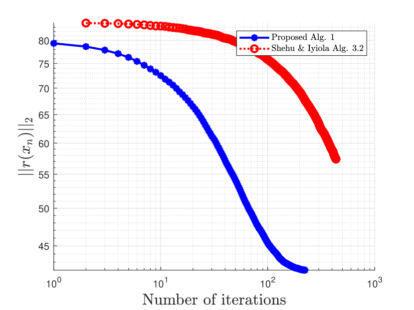
Figure 1: Example 5.1: $\gamma=0.01$, $N=10$

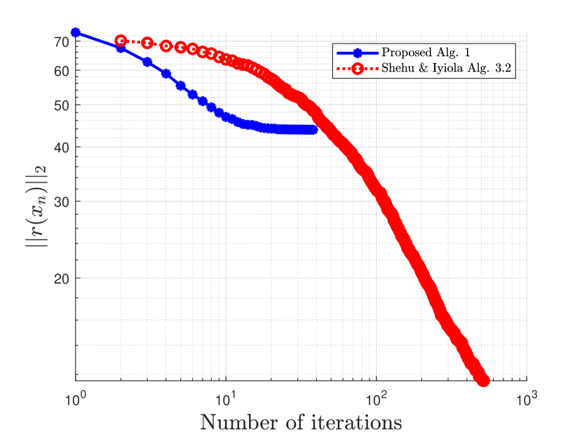
Figure 2: Example 5.1: $\gamma=0.1$, $N=10$

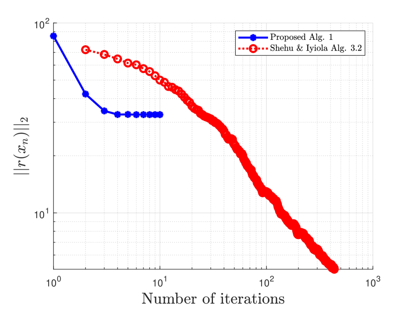
Figure 3: Example 5.1: $\gamma=0.5$, $N=10$

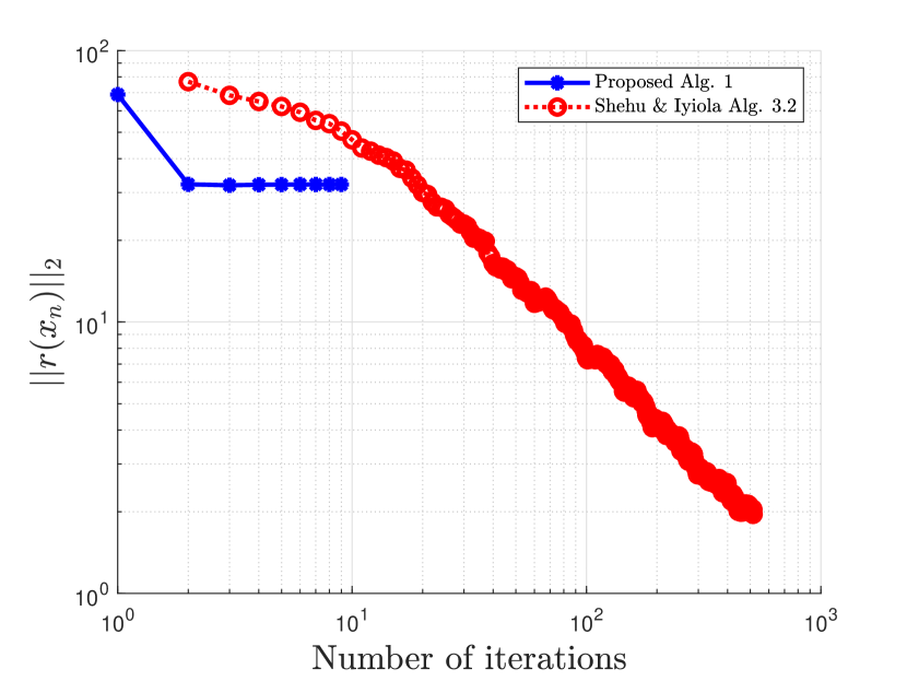
Figure 4: Example 5.1: $\gamma=0.7$, $N=10$

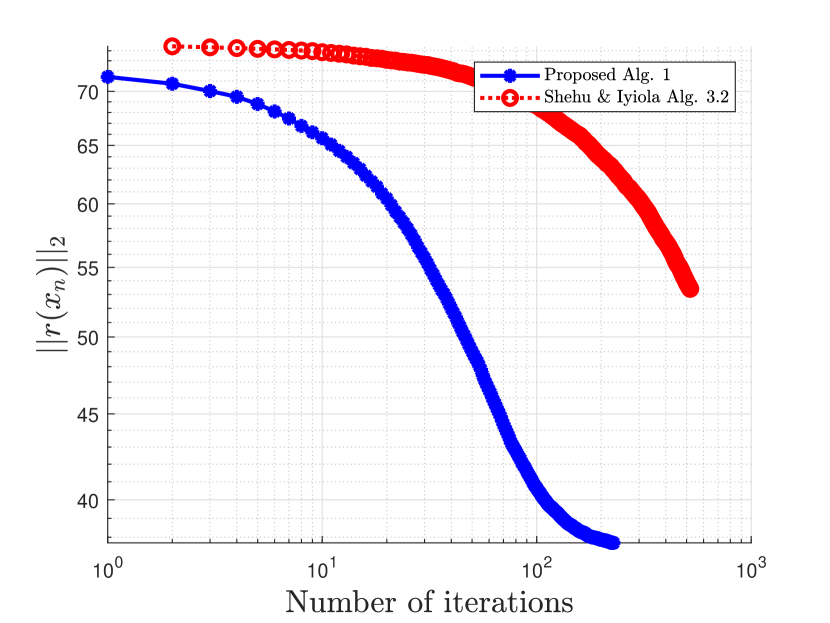
Figure 5: Example 5.1: $\gamma=0.01$, $N=20$

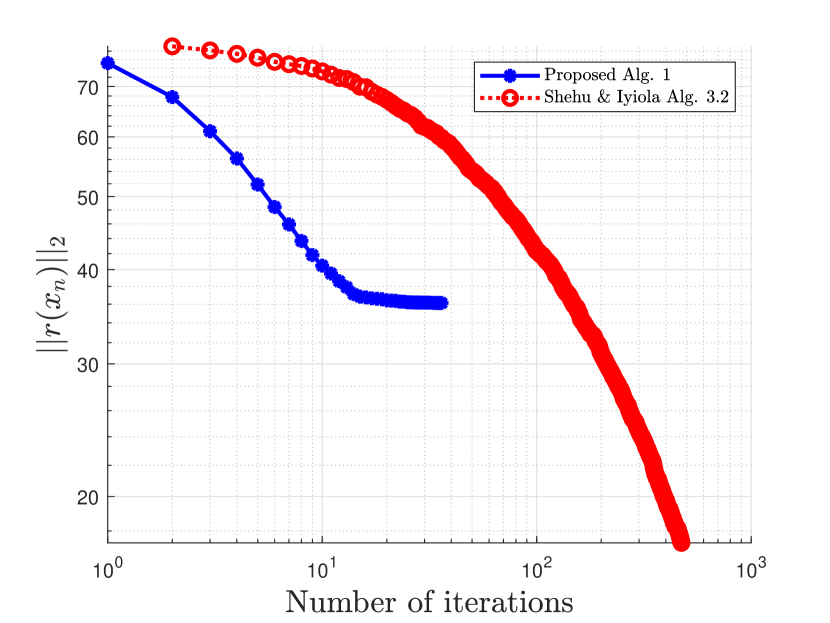
Figure 6: Example 5.1: $\gamma=0.1$, $N=20$

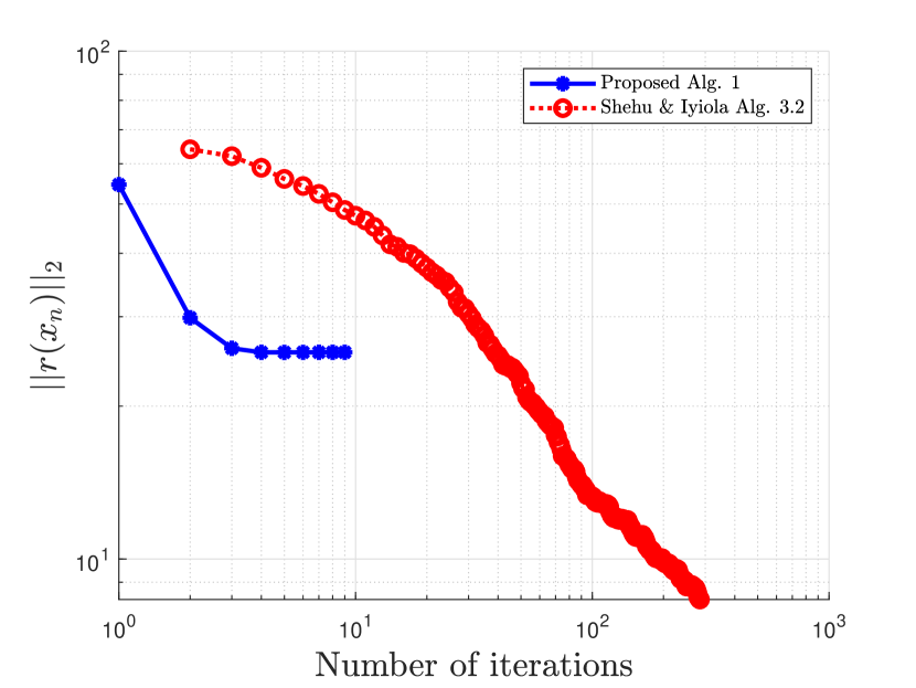
Figure 7: Example 5.1: $\gamma=0.5$, $N=20$

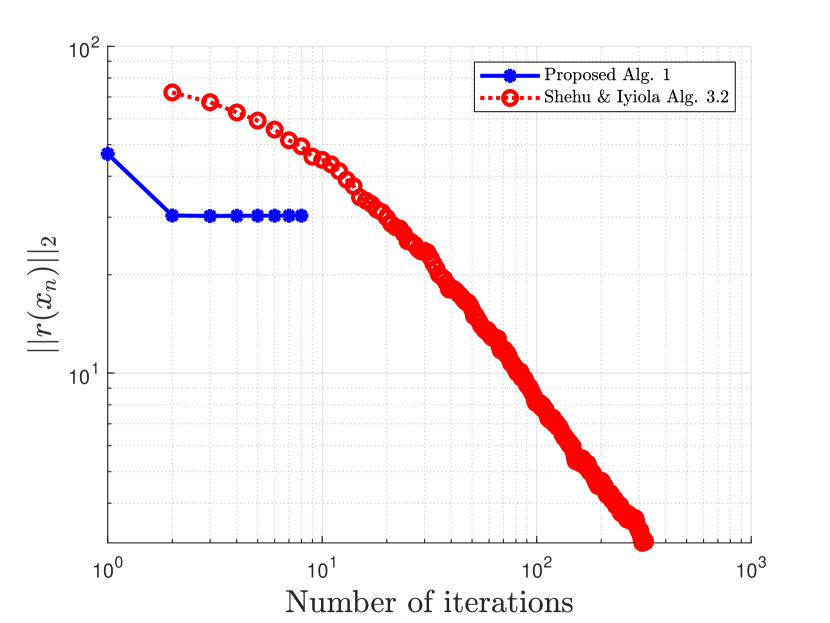
Figure 8: Example 5.1: $\gamma=0.7$, $N=20$

Example 5.2.

This example is taken from [27] and has been considered by many authors for numerical experiments (see, for example, [29, 42, 53]). The operator $A$ is defined by $A(x):=Mx+q$, where $M=BB^{T}+S+D$, with $B,S,D\in\mathbb{R}^{m\times m}$ randomly generated matrices such that $S$ is skew-symmetric (hence the operator does not arise from an optimization problem), $D$ is a positive definite diagonal matrix (hence the variational inequality has a unique solution) and $q=0$. The feasible set $C$ is described by linear inequality constraints $Bx\leq b$ for some random matrix $B\in\mathbb{R}^{k\times m}$ and a random vector $b\in\mathbb{R}^{k}$ with nonnegative entries. Hence the zero vector is feasible and therefore the unique solution of the corresponding variational inequality. These projections are computed using the MATLAB solver fmincon. Hence, for this class of problems, the evaluation of $A$ is relatively inexpensive, whereas projections are costly. We present the corresponding numerical results (number of iterations and CPU times in seconds) using six different dimensions $m$ and two different numbers of inequality constraints $k$.

We choose the stopping criterion as $\|x^{k}\|\leq\epsilon=0.001.$ The size $k=30,50$ and $m=10,20,30,40,50,60$. The matrices $B,S,D$ and the vector $b$ are generated randomly. We choose $\gamma=0.8$, $\sigma=0.5$, $\alpha_{n}=0.2$ in Algorithm (1). In (5), we choose $\sigma=0.8$, $\rho=0.1$, $\mu=0.2$. In (10), we choose $L=\|M\|$. Here, we compare our proposed Algorithm 1 with the subgradient extragradient method (SEM) (5), and the inertial subgradient extragradient method (Thong & Hieu) (10).

Table 2: Example 5.2 Comparison: Proposed Alg. 1 vs SEM (2) vs Thong & Hieu (3) (T & H (3))

		No. of Iterations				CPU time				Norm sol. ($10^{-3}$)
	$m$	Alg. 1	SEM (2)	T & H (3)		Alg. 1	SEM (2)	T & H (3)		Alg. 1	SEM (2)	T & H (3)
$k=30$	10	344	3867	4123		2.8707	31.5956	30.3300		0.99605	0.99927	0.99938
	20	747	14683	10493		5.6957	117.7458	84.7406		0.99608	0.99996	0.99984
	30	1777	31668	24968		13.891	269.2987	211.1937		0.99955	0.99999	0.99980
	40	2612	40224	36119		21.5972	358.3453	320.2933		0.99790	1.00000	0.99994
	50	3710	70321	51143		32.074	655.8354	469.0297		0.99981	0.99997	0.99995
	60	5619	56670	50619		50.4537	554.3951	491.5552		0.99929	0.99992	0.99998
$k=50$	10	200	6213	5518		1.90869	60.1212	47.6937		0.98471	0.99969	0.99945
	20	835	14354	10372		6.4942	126.429	96.9197		0.99909	0.99980	0.99991
	30	1978	25519	19357		16.4674	240.61	208.910		0.99794	0.99991	0.99990
	40	2832	47661	26790		30.3799	539.729	314.588		0.99734	0.99991	0.99938
	50	3933	43773	53055		45.8745	562.959	800.371		0.99985	0.99925	0.99999
	60	6025	97772	65820		100.304	1515.76	589.180		0.99955	0.99995	0.99994

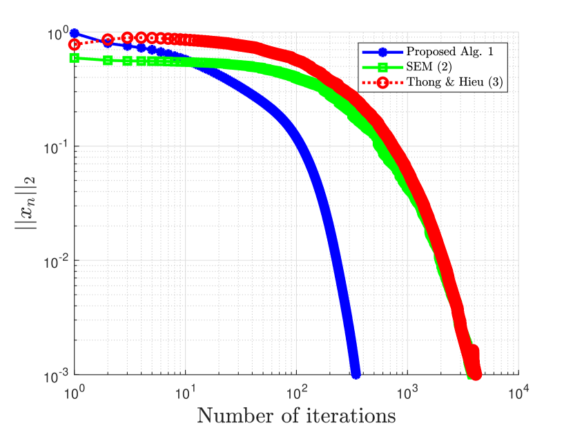
Figure 9: Example 5.2: $k=30$, $m=10$

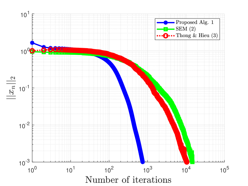
Figure 10: Example 5.2: $k=30$, $m=20$

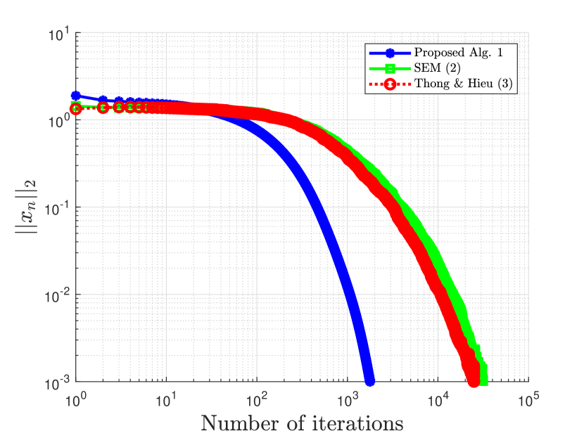
Figure 11: Example 5.2: $k=30$, $m=30$

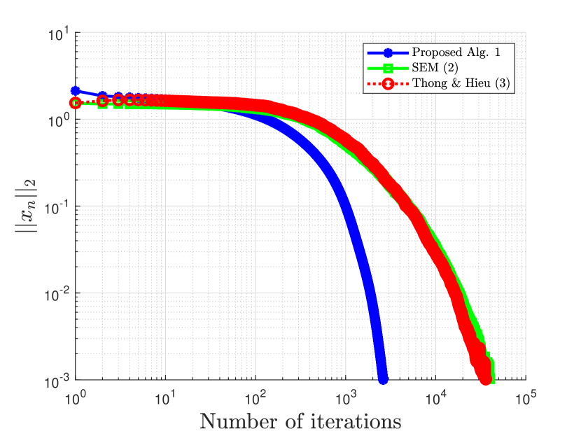
Figure 12: Example 5.2: $k=30$, $m=40$

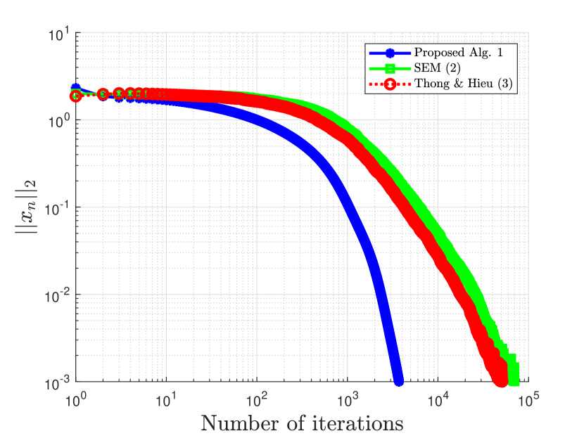
Figure 13: Example 5.2: $k=30$, $m=50$

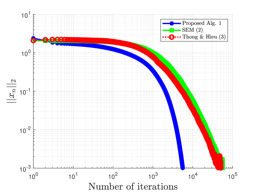
Figure 14: Example 5.2: $k=30$, $m=60$

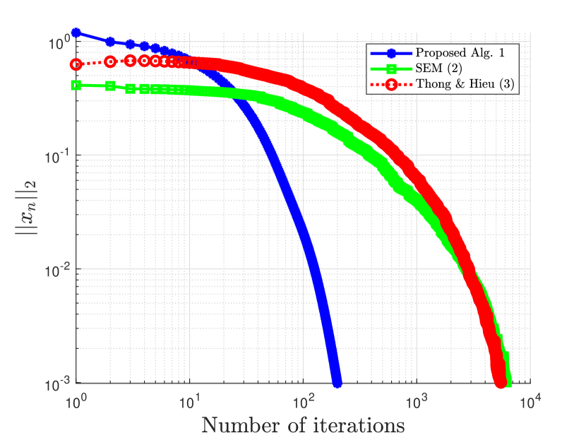
Figure 15: Example 5.2: $k=50$, $m=10$

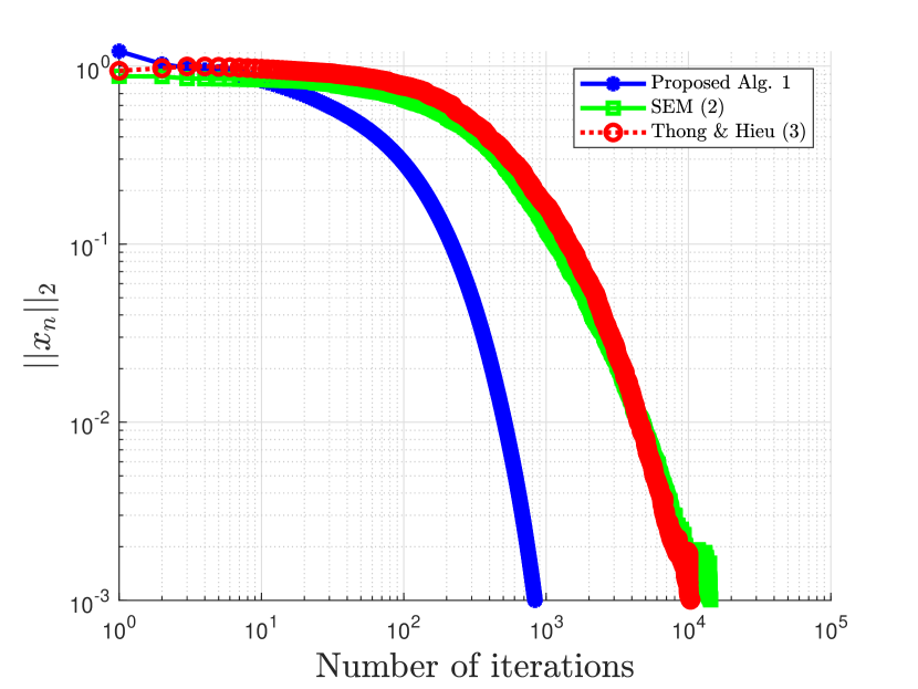
Figure 16: Example 5.2: $k=50$, $m=20$

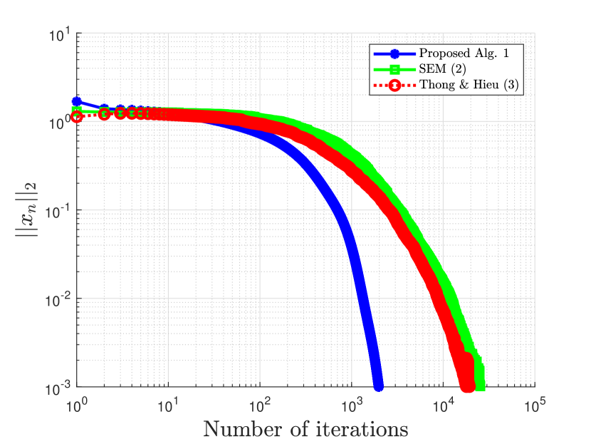
Figure 17: Example 5.2: $k=50$, $m=30$

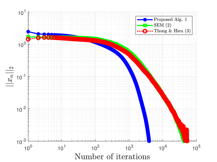
Figure 18: Example 5.2: $k=50$, $m=50$

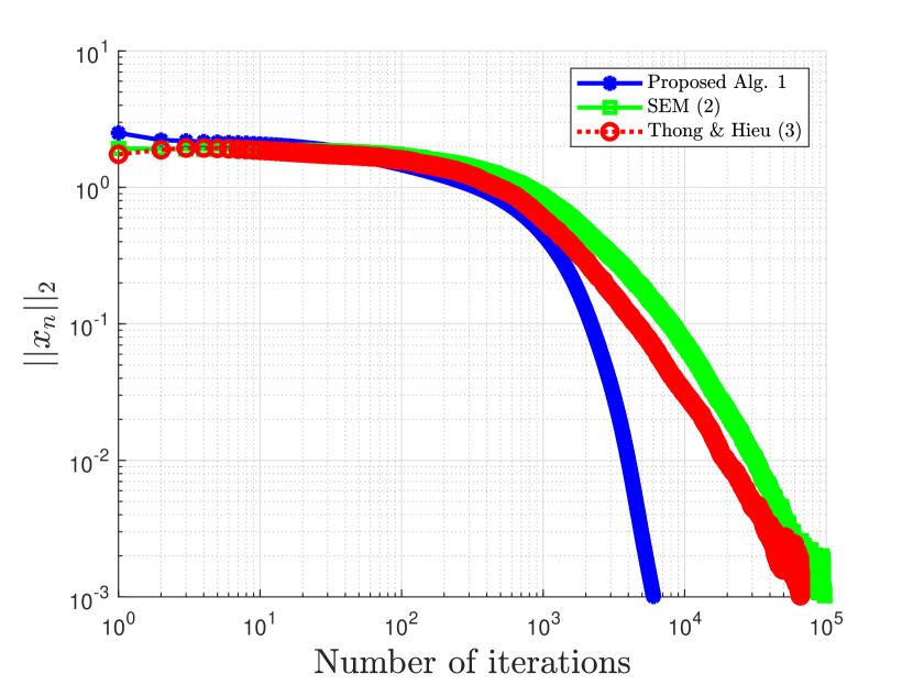
Figure 19: Example 5.2: $k=50$, $m=60$

Clearly, from both Examples, our proposed algorithm 1 outperforms and highly improves Shehu and Iyiola Algorithm (3.2) in [51], subgradient extragradient method (SEM) (5), and the inertial subgradient extragradient method (Thong & Hieu) (10) with respect to number of iterations required and CPU time and achieved norm of the solution. See Tables 1 - 2 and Figures 2 - 19.

We give an example in infinite dimensional Hilbert spaces. We give comparison of our proposed Algorithm 1 with Algorithm (5), Algorithm (10) and the non-inertial case of Algorithm 1 (when $\theta_{n}=0$).

Example 5.3.

Let $H:=L^{2}([0,1])$ with norm $\|x\|:=\Big{(}\int_{0}^{1}x(t)^{2}dt\Big{)}^{\frac{1}{2}}$ and inner product $\langle x,y\rangle:=\int_{0}^{1}x(t)y(t)dt,\leavevmode\nobreak\ \leavevmode\nobreak\ x,y\in H$. Let $C:=\{x\in L^{2}([0,1]):\int_{0}^{1}tx(t)dt=2\}$. Let us define the Volterra integral operator $F:L^{2}([0,1])\rightarrow L^{2}([0,1])$ by $Fx(t):=\int_{0}^{t}x(s)ds,\leavevmode\nobreak\ \leavevmode\nobreak\ x\in L^{2}([0,1]),t\in[0,1]$. Then, $F$ is monotone, bounded and linear with $L=\frac{2}{\pi}$ (see Exercises 20.12 of [9]) . Observe that $\text{SOL}\neq\emptyset$ since $0\in\text{SOL}$. Observe that (see [15])

$$P_{C}(x)(t):=x(t)-\frac{\int_{0}^{1}tx(t)dt-2}{\int_{0}^{1}t^{2}dt}t,\leavevmode\nobreak\ \leavevmode\nobreak\ t\in[0,1].$$

6 Final Remarks

We propose an inertial projection method for solving variational inequality problem and give weak convergence result. The cost function is assumed to be monotone and non-Lipschitz continuous. Our numerical implementations show that our method is more efficient and outperforms some other related methods in the literature. Our result is more applicable than the results on variational inequality where the Lipschitz constant of the cost function is needed. Our future project is focused on how to extend the range of inertial factor $\alpha_{n}$ beyond $1/3$ and extend our results to infinite dimensional Banach spaces.

Disclosure statement

No potential conflict of interest was reported by the author(s).

Funding

The project of the first author has received funding from the European Research Council (ERC) under the European Union’s Seventh Framework Program (FP7 - 2007-2013) (Grant agreement No. 616160).

References

• [1] F. Alvarez, Weak convergence of a relaxed and inertial hybrid projection-proximal point algorithm for maximal monotone operators in Hilbert space. SIAM J. Optim. 14 (2004), 773-782.
• [2] F. Alvarez and H. Attouch; An inertial proximal method for maximal monotone operators via discretization of a nonlinear oscillator with damping, Set-Valued Anal. 9 (2001), 3-11.
• [3] H. Attouch, X. Goudon and P. Redont; The heavy ball with friction. I. The continuous dynamical system, Commun. Contemp. Math. 2 (1) (2000), 1-34.
• [4] H. Attouch and M.O.  Czarnecki; Asymptotic control and stabilization of nonlinear oscillators with non-isolated equilibria, J. Differential Equations 179 (1) (2002), 278-310.
• [5] H. Attouch, J.  Peypouquet and P. Redont; A dynamical approach to an inertial forward-backward algorithm for convex minimization, SIAM J. Optim. 24 (2014), 232-256.
• [6] H. Attouch and J. Peypouquet; The rate of convergence of Nesterov’s accelerated forward-backward method is actually faster than $\frac{1}{k^{2}}$, SIAM J. Optim. 26 (2016), 1824-1834.
• [7] J.-P. Aubin and I. Ekeland; Applied Nonlinear Analysis, Wiley, New York, 1984.
• [8] C. Baiocchi and A. Capelo; Variational and Quasivariational Inequalities; Applications to Free Boundary Problems, Wiley, New York (1984).
• [9] H.H. Bauschke and P.L. Combettes; Convex Analysis and Monotone Operator Theory in Hilbert Spaces, CMS Books in Mathematics, Springer, New York (2011).
• [10] A.  Beck and M. Teboulle; A fast iterative shrinkage-thresholding algorithm for linear inverse problems, SIAM J. Imaging Sci. 2 (1) (2009), 183-202.
• [11] R. I.  Bot, E. R. Csetnek and C.  Hendrich; Inertial Douglas-Rachford splitting for monotone inclusion, Appl. Math. Comput. 256 (2015), 472-487.
• [12] R. I. Bot and E. R. Csetnek; An inertial alternating direction method of multipliers, Minimax Theory Appl. 1 (2016), 29-49.
• [13] R. I. Bot and E. R. Csetnek; An inertial forward-backward-forward primal-dual splitting algorithm for solving monotone inclusion problems, Numer. Alg. 71 (2016), 519-540.
• [14] X. Cai, G. Gu and B. He; On the $O(1/t)$ convergence rate of the projection and contraction methods for variational inequalities with Lipschitz continuous monotone operators, Comput. Optim. Appl. 57 (2014), 339-363.
• [15] A. Cegielski; Iterative Methods for Fixed Point Problems in Hilbert Spaces, Lecture Notes in Mathematics 2057, Springer, Berlin, 2012.
• [16] L.C. Ceng, N. Hadjisavvas, and N.-C. Wong; Strong convergence theorem by a hybrid extragradient-like approximation method for variational inequalities and fixed point problems, J. Glob. Optim. 46 (2010), 635-646.
• [17] L. C. Ceng and J. C. Yao; An extragradient-like approximation method for variational inequality problems and fixed point problems, Appl. Math. Comput. 190 (2007), 205-215.
• [18] Y. Censor, A. Gibali, and S. Reich; Strong convergence of subgradient extragradient methods for the variational inequality problem in Hilbert space, Optim. Methods Softw. 26 (2011), 827-845.
• [19] Y. Censor, A. Gibali and S. Reich; The subgradient extragradient method for solving variational inequalities in Hilbert space, J. Optim. Theory Appl. 148 (2011), 318-335.
• [20] C. Chen, R. H.  Chan, S.  Ma and J.  Yang; Inertial Proximal ADMM for Linearly Constrained Separable Convex Optimization, SIAM J. Imaging Sci. 8 (2015), 2239-2267.
• [21] S. Denisov, V. Semenov and L. Chabak; Convergence of the modified extragradient method for variational inequalities with non-Lipschitz operators, Cybernet. Systems Anal. 51 (2015), 757-765.
• [22] Q. L. Dong, Y. J. Cho, L. L. Zhong and Th. M. Rassias; Inertial projection and contraction algorithms for variational inequalities, J. Global Optim. 70 (2018), 687-704.
• [23] G. Fichera; Sul problema elastostatico di Signorini con ambigue condizioni al contorno, Atti Accad. Naz. Lincei, VIII. Ser., Rend., Cl. Sci. Fis. Mat. Nat. 34 (1963), 138-142.
• [24] G. Fichera; Problemi elastostatici con vincoli unilaterali: il problema di Signorini con ambigue condizioni al contorno, Atti Accad. Naz. Lincei, Mem., Cl. Sci. Fis. Mat. Nat., Sez. I, VIII. Ser. 7 (1964), 91-140.
• [25] R. Glowinski, J.-L. Lions, and R. Trémolières; Numerical Analysis of Variational Inequalities, North-Holland, Amsterdam (1981).
• [26] K. Goebel and S. Reich; Uniform convexity, hyperbolic geometry, and nonexpansive mappings, Marcel Dekker, New York, (1984).
• [27] P. T. Harker, and J.-S. Pang; A damped-Newton method for the linear complementarity problem, in Computational Solution of Nonlinear Systems of Equations, Lectures in Appl. Math. 26, G. Allgower and K. Georg, eds., AMS, Providence, RI, 1990, pp. 265-284.
• [28] Y. R. He; A new double projection algorithm for variational inequalities, J. Comput. Appl. Math. 185 (2006), 166-173.
• [29] D. V. Hieu, P. K. Anh and L. D. Muu; Modified hybrid projection methods for finding common solutions to variational inequality problems, Comput. Optim. Appl. 66 (2017), 75-96
• [30] A.N. Iusem and R. Gárciga Otero; Inexact versions of proximal point and augmented Lagrangian algorithms in Banach spaces, Numer. Funct. Anal. Optim. 22 (2001), 609-640.
• [31] A.N. Iusem and M. Nasri; Korpelevich’s method for variational inequality problems in Banach spaces, J. Global Optim. 50 (2011), 59-76.
• [32] C. Kanzow, Y. Shehu; Strong convergence of a double projection-type method for monotone variational inequalities in Hilbert spaces, J. Fixed Point Theory Appl. 20 (2018), Article 51.
• [33] E.N. Khobotov; Modification of the extragradient method for solving variational inequalities and certain optimization problems, USSR Comput. Math. Math. Phys. 27 (1989), 120-127.
• [34] D. Kinderlehrer and G. Stampacchia; An Introduction to Variational Inequalities and Their Applications, Academic Press, New York (1980).
• [35] I.V. Konnov; Combined Relaxation Methods for Variational Inequalities, Springer-Verlag, Berlin (2001).
• [36] G.M. Korpelevich; The extragradient method for finding saddle points and other problems, Ékon. Mat. Metody 12 (1976), 747-756.
• [37] D. A.  Lorenz and T.  Pock; An inertial forward-backward algorithm for monotone inclusions, J. Math. Imaging Vis., 51 (2015), 311-325.
• [38] P. E. Maing$\acute{e}$; Regularized and inertial algorithms for common fixed points of nonlinear operators, J. Math. Anal. Appl. 344 (2008), 876-887.
• [39] P.-E. Maingé; A hybrid extragradient-viscosity method for monotone operators and fixed point problems, SIAM J. Control Optim. 47 (2008), 1499-1515.
• [40] P.-E. Maingé and M.L. Gobinddass; Convergence of one-step projected gradient methods for variational inequalities, J. Optim. Theory Appl. 171 (2016), 146-168.
• [41] Yu.V. Malitsky; Projected reflected gradient methods for monotone variational inequalities, SIAM J. Optim. 25 (2015), 502-520.
• [42] Yu.V. Malitsky and V.V. Semenov; A hybrid method without extrapolation step for solving variational inequality problems, J. Global Optim. 61 (2015), 193-202.
• [43] P.  Marcotte; Applications of Khobotov’s algorithm to variational and network equlibrium problems, Inf. Syst. Oper. Res. 29 (1991), 258-270.
• [44] J. Mashreghi and M. Nasri; Forcing strong convergence of Korpelevich’s method in Banach spaces with its applications in game theory, Nonlinear Analysis 72 (2010), 2086-2099.
• [45] N. Nadezhkina and W. Takahashi; Strong convergence theorem by a hybrid method for nonexpansive mappings and Lipschitz-continuous monotone mappings, SIAM J. Optim. 16 (2006), 1230-1241.
• [46] P.  Ochs, T.  Brox and T.  Pock; iPiasco: Inertial Proximal Algorithm for strongly convex Optimization, J. Math. Imaging Vis. 53 (2015), 171-181.
• [47] B. T.  Polyak; Some methods of speeding up the convergence of iterarive methods, Zh. Vychisl. Mat. Mat. Fiz. 4 (1964), 1-17.
• [48] L. D. Popov; A modification of the Arrow-Hurwicz method for searching for saddle points, Mat. Zametki. 28 (1980), 777-784.
• [49] Y. Shehu, O. S. Iyiola, X.-H. Li, Q.-L. Dong; Convergence analysis of projection method for variational inequalities, Comp. Appl. Math. 38: 161 (2019).
• [50] Y. Shehu and O. S. Iyiola; On a modified extragradient method for variational inequality problem with application to industrial electricity production, J. Ind. Manag. Optim. 15 (2019), 319-342.
• [51] Y. Shehu and O. S. Iyiola; Iterative algorithms for solving fixed point problems and variational inequalities with uniformly continuous monotone operators, Numerical Algorithms 79(2) (2018), 529-553.
• [52] Y. Shehu and P. Cholamjiak; Iterative method with inertial for variational inequalities in Hilbert spaces, Calcolo 56 (2019), no. 1, Art. 4, 21 pp.
• [53] M.V. Solodov and B.F. Svaiter; A new projection method for variational inequality problems, SIAM J. Control Optim. 37 (1999), 765-776.
• [54] W. Takahashi; Nonlinear Functional Analysis, Yokohama Publishers, Yokohama, (2000).
• [55] D. V.  Thong and D. V.  Hieu; Modified subgradient extragradient method for variational inequality problems. In press: Numer. Algor. doi:10.1007/s11075-017-0452-4.
• [56] P. Tseng; A modified forward-backward splitting method for maximal monotone mappings, SIAM J. Control Optim. 38 (2000), 431-446.
• [57] G. L. Xue and Y. Y. Ye; An efficient algorithm for minimizing a sum of Euclidean norms with applications, SIAM J. Optim. 7 (1997), 1017-1036.
• [58] L. H. Yen · L.D. Muu and N. T. T. Huyen; An algorithm for a class of split feasibility problems: application to a model in electricity production, Math. Meth. Oper. Res. 84 (2016), 549-565.