Effects of dynamical screening on the BCS-BEC crossover in double bilayer graphene: Density functional theory for exciton bilayers

Abstract

We derive a gap equation for bilayer excitonic systems based on density functional theory and benchmark our results against quantum Monte-Carlo simulations and recent experiments on double bilayer graphene. The gap equation has a mean-field form but includes a consistent treatment of dynamical screening. We show that the gap survives at much higher densities than previously thought from mean-field estimates which gives strong indications that the double-bilayer graphene systems at zero magnetic field can be used as model systems to investigate the BCS-BEC crossover. Furthermore, we show that Josephson-like transfer of pairs can be substantial for small band gaps and densities.

In a recent experiment Burg et al. (2018) on two bilayer graphene sheets separated by a WSe₂ insulating barrier an enhanced tunneling rate was measured, which indicates the formation of an exciton condensate. While exciton formation has previously been achieved in similar systems in the quantum Hall regime at high magnetic fields Liu et al. (2017); Li et al. (2017) these were the first experimental indications of exciton formation in bilayer systems at zero magnetic field. In bilayer graphene systems the electron and hole concentrations are tunable by metallic gates, which opens up for the possibility to tune the device from the Bose-Einstein condensate (BEC) to the Bardeen-Cooper-Schrieffer (BCS) regime with possible applications in novel electronic devices Banerjee et al. (2009).

Theoretically, bilayer excitonic systems are typically described within mean-field theory Lozovik et al. (2012); Perali et al. (2013); Zarenia et al. (2014); Neilson et al. (2014); Conti et al. (2017, 2019) or using Quantum Monte-Carlo (QMC) simulations De Palo et al. (2002); Maezono et al. (2013); López Ríos et al. (2018). While the latter is very accurate the calculations are restricted to simplified single-band systems which partly limit the predictive power. The mean-field calculations, on the other hand, can be applied to realistic systems but neglect dynamical screening as well as higher order self-energy diagrams and are therefore, as we will argue below, only accurate in the low-density limit. The role of dynamical screening for single bilayer graphene systems and topological insulators was previously investigated in Ref. Sodemann et al. (2012) by solving the imaginary axis gap equation. Similar to the present work it was shown that a static mean-field description severely underestimates the gap in a large parameter regime. In this letter we derive a new gap equation, based on density functional theory, which yields an effective account of dynamical screening at a sufficiently low computational cost to be applied to realistic materials. The method is applied to double bilayer graphene, which is the most promising bilayer candidate for achieving exciton condensation without an applied magnetic field. To our knowledge this is the first time that the effect of dynamical screening is studied for realistic multiband models of this material. We begin by giving a brief account of the derivation (the complete derivation is given in the supplemental material (SM)), then we benchmark our method against QMC simulations for simplified models López Ríos et al. (2018) and finally consider realistic systems where we compare to the experimental results in Ref. Burg et al. (2018) and mean-field calculations in Ref. Conti et al. (2019). We show that, contrary to mean-field theories, the results from our effective gap equation qualitatively agree both with QMC simulations and experimental measurements. Due to its low computational cost the theory can provide an efficient means to predict exciton condensation in novel materials and an important complement to existing methods.

We start with the Kohn-Sham Hamiltonian for the electron-hole system

$$\hat{H}_{KS}= \int dr\hat{\psi}^{\dagger}(r)H^{e}(r)\hat{\psi}(r)+\int dr\hat{\phi}^{\dagger}(r)H^{h}(r)\hat{\phi}(r)$$

$$-\int drdr^{\prime}\Delta(r,r^{\prime})\hat{\psi}^{\dagger}(r)\hat{\phi}^{\dagger}(r^{\prime})+h.c.$$ (1)

Here $\psi(r)$ ($\phi(r)$) are the electron (hole) field operators and $\Delta(r,r^{\prime})$ is the Kohn-Sham electron-hole potential. Assuming band diagonal phase-coherent singlet coupling (i.e. electrons of spin $\sigma$, ,momentum $k$ and band $\gamma$ couple to holes with spin $-\sigma$ momentum $-k$ and band $\gamma$) the Hamiltonian can be rewritten as

$$H_{KS}= \sum_{k,\gamma}\varepsilon_{k\gamma}^{h}\hat{a}^{\dagger}_{k\gamma}\hat{a}_{k\gamma}+\sum_{k\gamma}\varepsilon_{k\gamma}^{e}\hat{b}^{\dagger}_{k\gamma}\hat{b}_{k\gamma}$$

$$- \sum_{k\gamma}\Delta_{k\gamma}\hat{a}^{\dagger}_{k\gamma}\hat{b}^{\dagger}_{-k\gamma}+h.c.$$ (2)

Here $\varepsilon_{k\gamma}^{e/h}$ are the eigenenergies of $H^{e/h}$, $\hat{b}^{\dagger}$ and $\hat{a}^{\dagger}$ are the corresponding creation operators and $\Delta_{k\gamma}$ is the matrix element of $\Delta(r,r^{\prime})$ in the electron and hole eigenstates (see SM). This approximation is the analogue of the decoupling approximation in superconductor density functional theory (scDFT). For graphene bilayers in AB-stacking a tight-binding fit to the low-energy band structure is given by Partoens and Peeters (2006); McCann and Koshino (2013); Conti et al. (2019)

$$\varepsilon_{k\gamma}=\frac{\gamma}{2}\sqrt{(t_{1}-\Gamma_{k})^{2}+\Omega_{k}}-\mu$$ (3)

where

$$\Gamma_{k}=\sqrt{t_{1}^{2}+(2\hbar vk)^{2}+(2E_{g}\hbar vk)^{2}/t_{1}^{2}},$$

$$\Omega_{k}=E_{g}^{2}(1-(2\hbar vk)^{2}/t_{1}^{2}),$$

$$v=\sqrt{3}at_{0}/2\hbar$$

Unless otherwise specified we use the bilayer bandstructure above with the intercell distance $a=0.246$nm, intralayer hopping $t_{0}=3.16$eV and interlayer hopping $t_{1}=0.38$eV Kuzmenko et al. (2009); Conti et al. (2019) for both the electron and hole layers. For simplicity we will assume $\varepsilon^{e}_{k\gamma}=\varepsilon^{h}_{-k\gamma}=\varepsilon_{k\gamma}$ in the derivation below, although it is straight-forward to generalize the derivation to different electron and hole dispersions. All calculations were performed at a temperature of 1.5 K. The Hamiltonian in Eq. 2 is diagonalized by a Bogoliubov transformation

$$\hat{b}_{k\gamma}=u_{k\gamma}\hat{\alpha}_{k\gamma}+v_{k\gamma}\hat{\beta}^{\dagger}_{-k\gamma}$$ (4)

$$\hat{a}_{k\gamma}=u_{k\gamma}\hat{\beta}_{k\gamma}-v_{k\gamma}\hat{\alpha}^{\dagger}_{-k\gamma}.$$ (5)

The amplitudes $u_{k\gamma}$ and $v_{k\gamma}$ are subject to the equations

$$u_{k\gamma}^{2}=\frac{1}{2}(1+\frac{\xi_{k\gamma}}{\tilde{E}_{k\gamma}})$$ (6)

$$v_{k\gamma}^{2}=\frac{1}{2}(1-\frac{\xi_{k\gamma}}{\tilde{E}_{k\gamma}})$$ (7)

$$2u_{k\gamma}v_{k\gamma}=\pm\Delta_{k\gamma}/E_{k\gamma},$$ (8)

where $\tilde{E}_{k\gamma}=\pm E_{k\gamma}$, $E_{k\gamma}=\sqrt{\varepsilon_{k\gamma}^{2}+\Delta_{k\gamma}^{2}}$. We define the Kohn-Sham propagators

$$G^{e}(r\tau,r^{\prime}\tau^{\prime}) =-\langle\hat{T}\hat{\psi}(r\tau)\hat{\psi}^{\dagger}(r^{\prime}\tau^{\prime})\rangle_{KS},$$ (9)

$$G^{h}_{KS}(r\tau,r^{\prime}\tau^{\prime}) =-\langle\hat{T}\hat{\phi}^{\dagger}(r\tau)\hat{\phi}(r^{\prime}\tau^{\prime})\rangle_{KS},$$ (10)

$$F^{eh}_{KS}(r\tau,r^{\prime}\tau^{\prime}) =-\langle\hat{T}\hat{\psi}(r\tau)\hat{\phi}(r^{\prime}\tau^{\prime})\rangle_{KS}.$$ (11)

Utilizing the the decoupling approximation and Fourier transforming to frequency space yields

$$G^{e}_{k\gamma}(\omega_{n})=\frac{u_{k}^{2}}{i\omega_{n}-\varepsilon_{\gamma k}}+\frac{v_{k}^{2}}{i\omega_{n}+\varepsilon_{\gamma k}}$$ (12)

$$G^{h}_{k\gamma}(\omega_{n})=\frac{u_{k}^{2}}{i\omega_{n}+\varepsilon_{\gamma k}}+\frac{v_{k}^{2}}{i\omega_{n}-\varepsilon_{\gamma k}}$$ (13)

$$F^{eh}_{k\gamma}(\omega_{n})=\frac{v_{k}^{*}u_{k}}{i\omega_{n}-\epsilon_{\gamma k}}-\frac{u_{k}v_{k}^{*}}{i\omega_{n}+\epsilon_{\gamma k}},$$ (14)

Using the Sham-Schlüter connection Godby et al. (1986, 1987a, 1987b) with the same approximations as in scDFT Lüders et al. (2005); Lüders and Gross (1999); Marques and Gross (2000) one can then derive the gap equation for the Kohn-Sham system

$$\Delta_{k\gamma}=\frac{\sum_{\omega_{n}}\Sigma^{a}_{k\gamma}(\omega_{n})G^{h}_{k\gamma}(\omega_{n})G^{e}_{k\gamma}(\omega_{n})]}{\sum_{\omega_{n}}[G^{h}_{k\gamma}(\omega_{n})G^{e}_{k\gamma}(\omega_{n})]}$$ (15)

where $\Sigma^{a}$ is the exchange-correlation part of the anomalous self-energy and we have assumed that the effect of the normal self-energies are included in the bare dispersion. A generalized gap equation which include also the electron-electron and hole-hole correlations is given in the SM. It is straight-forward to show that a static exchange approximation to the self-energy yields the usual mean-field gap equation

$$\Delta_{k\gamma}=-\sum_{k^{\prime},\gamma^{\prime}}\mathcal{F}_{kk^{\prime}}^{\gamma\gamma^{\prime}}\frac{V_{k-k^{\prime}}\Delta_{\gamma^{\prime}k^{\prime}}}{2E_{\gamma^{\prime}k^{\prime}}}(1-f_{\beta}(\epsilon_{\gamma^{\prime}k^{\prime}+})-f_{\beta}(\epsilon_{\gamma^{\prime}k^{\prime}-})).$$ (16)

The geometrical form-factor $\mathcal{F}$ is related to the overlap of the single particle states $|\Psi_{k\gamma}\rangle\equiv|f_{k\gamma}\rangle e^{i\mathbf{k}\mathbf{r}}$ as $\mathcal{F}_{kk^{\prime}}^{\gamma\gamma^{\prime}}=\langle f_{k,\gamma}|f_{k^{\prime},\gamma^{\prime}}\rangle\langle f_{k^{\prime},\gamma^{\prime}}|f_{k,\gamma}\rangle$ Lozovik and Sokolik (2010) (See the SM for details).

In order to include the effect of dynamical screening we compute $\Sigma^{a}$ in Eq. 15 within the $GW$-approximation

$$\Sigma^{a}_{k\gamma}(i\omega_{n})=\sum_{k^{\prime},\gamma^{\prime},\nu_{l}}\mathcal{F}_{k,k-k^{\prime}}^{\gamma\gamma^{\prime}}F^{eh}_{k-k^{\prime},\gamma}(i\omega_{n}-i\nu_{l})W^{eh}_{k^{\prime}}(\nu_{l})$$ (17)

The screened electron-hole interaction for the bilayer system is given by Lozovik et al. (2012); Sodemann et al. (2012); Conti et al. (2019)

$$W^{eh}=\frac{-V_{D}-\Pi_{a}(V^{2}-V_{D}^{2})}{1-2(V\Pi_{n}+V_{D}\Pi_{a})+(\Pi_{n}^{2}-\Pi_{a}^{2})(V^{2}-V_{D}^{2})},$$ (18)

where the $k$ and Matsubara indexes are implicit for all quantities and

$$V=V_{k}=\frac{2\pi e^{2}}{\epsilon}\frac{1}{|\mathbf{k}|}$$ (19)

$$V_{D}=V^{D}_{k}=e^{-dk}\frac{2\pi e^{2}}{\epsilon}\frac{1}{|\mathbf{k}|}.$$ (20)

Unless otherwise specified we use the dielectric constant $\epsilon=2$ for bilayer graphene sheets in a few layers of hexagonal boron nitride Kumar et al. (2016); Conti et al. (2019). $\Pi_{n}=\Pi^{(n)}_{q}(i\nu_{n})$ and $\Pi_{a}=\Pi^{(a)}_{q}(i\nu_{n})$ are the normal and anomalous polarizations which are computed within the random-phase approximation (See SM).

In order to have an efficient implementation at low temperatures all Matsubara sums have to be done analytically. This is straightforward for the polarizations, but for the self-energy in Eq. 17 it is not as clear. In this work we adopt a similar strategy as Ref. Akashi and Arita, 2013 and fit $W^{eh}_{k}(\nu_{l})$ to a multiple plasmon pole model

$$\tilde{W}_{k}^{eh}(i\nu_{m})=W_{k}^{eh}(0)+\sum_{i}^{N_{p}}a_{i;k}\left(\frac{2}{\omega_{i;k}}-\frac{2\omega_{i;k}}{\nu_{m}^{2}+\omega_{i;k}^{2}}\right).$$ (21)

We use up to 100 poles in order to get the correct shape of the peaks in Im$W^{eh}$. The position of the main pole and the relative weight of the poles are determined by the analytical continuation of $W^{eh}(i\nu_{n})$ to the real axis, while the overall weight of the poles is determined by a least square fit of the imaginary axis data. We evaluated all Matsubara sums in Eqs. 15 and 17 analytically using the MatsubaraSum package for Mathematica Mat . The details of the fitting procedure are given in the SM.

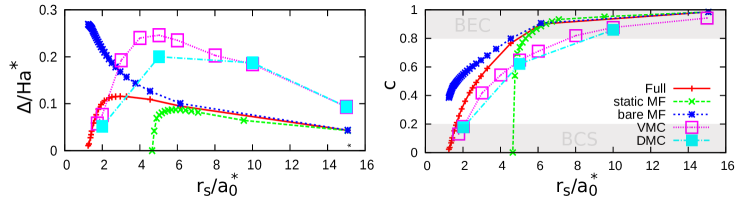
Figure 1: Maximum value of the superfluid gap (left) and condensate fraction (right) for a single band model with parabolic bands as a function of $r_{s}/a_{0}^{*}$ where $r_{s}=\sqrt{1/(\pi n)}$ and $a_{0}^{*}=\kappa(m_{e}/m_{e}^{*})a_{0}$. The variational quantum Monte Carlo (VMC) and diffusion Quantum Monte-Carlo (DMC) data are taken from Ref. López Ríos et al., 2018.

To benchmark our method we first consider a model with single parabolic electron and hole bands and compare with the Quantum Monte-Carlo simulations by Rìos et. al López Ríos et al. (2018). In Fig. 1 we compare the results from solving the full DFT gap equation (Eq. 15), the standard mean-field gap equation (Eq. 16) with the static value of the screened interaction (screened MF-equation) and the same equation but with the unscreened value of the interaction (bare MF-equation) with the corresponding results from the QMC simulations in Ref. López Ríos et al., 2018. The screened MF equation was benchmarked against QMC previously, with encouraging results Neilson et al. (2014). However, in these calculations a different form of the screened interaction was used and the formfactor was ignored in the gap equation. As we will see below, a correct treatment of the interaction and formfactor yields a larger screening and substantially worsens the performance of the screened MF equation. We begin by considering the maximum value of the gap. To facilitate the comparison we adopt the scaled units of Ref. López Ríos et al., 2018 with the effective energy unit Ha${}^{*}=m_{e}^{*}/m_{e}\kappa^{-2}$Ha and distances in units of $a_{0}^{*}=\kappa(m_{e}/m_{e}^{*})a_{0}$. The density $n$ is defined through $r_{s}/a_{0}^{*}$ where $r_{s}=\sqrt{1/(\pi n)}$. We use the same interlayer distance $d/a_{0}^{*}=0.4$. In Ref. López Ríos et al., 2018 the gap was estimated by fitting the excitation energies $E(k)$ obtained from the QMC simulations to an effective mean-field gap-equation with $k$-independent gap

$$E(k)=\sqrt{(k^{2}/2m^{*}-\mu)^{2}+\Delta^{2}}$$

with $m^{*}$, $\mu$ and $\Delta$ as fitting variables. In our simulations we use the effective mass which gave the optimal fit for each density (extracted from Fig. 3 in Ref López Ríos et al., 2018) and consider the maximum value of the $k$-dependent gap.

At low densities (high $r_{s}/a_{0}^{*}$) all mean-field calculations yield the same gap (left panel in Fig. 1). As the density is increased the screening reduces the gap of the screened MF result compared to the bare MF results substantially and at $r_{s}/a_{0}^{*}\approx 4.5$ the screened mean-field gap rapidly goes to zero. The additional correction in the DFT gap equation reduces the screening and increases the gap compared to the static MF results, while it is always smaller than the corresponding value in the bare MF calculation. Hence the DFT gap equation incorporates the frequency dependence of the interaction in an effective static theory, similar to the $Z$-factor approach for Hubbard models Casula et al. (2012). Due to the decrease of the effective screening the full gap goes to zero around $r_{s}/a_{0}^{*}\approx 1.2-2$, which corresponds to much higher densities than the static MF gap and is in qualitative agreement with the QMC results. At low and intermediate densities ($r_{s}/a_{0}^{*}>4$) all mean-field calculations underestimate the gap compared to the QMC data. Since the bare MF calculations sets the upper limit of $\Delta$ obtainable by any mean-field approximation relying on the first-order diagram of $\Sigma$, this indicates that the differences at low density may originate from many-body effects beyond a first-order mean-field description. Both the screened mean-field and DFT gap equation are restricted to the first-order term of the self-energy expansion in $W^{eh}$. This is a good approximation as long as $W^{eh}$ is sufficiently small or equivalently the screening is large, which explains why the DFT gap-equation agrees better with the QMC data for high densities than for intermediate and low densities. Thus, the poor performance of the screened MF equation for high densities is related to the neglect of the frequency dependence of the interaction, which is to a large extent cured by the effective treatment in the DFT gap-equation. The mean-field treatments give reasonable results also in the low-density limit, which is expected since the mean-field treatment becomes exact in the limit $n\rightarrow 0$. It should be noted that the DFT gap-equation (Eq. 15) is not restricted to the $GW$-approximation for the self-energy, and hence in principle higher order self-energy terms can be accounted for within our framework.

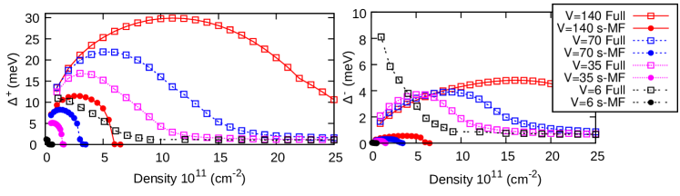
Figure 2: Maximum superfluid gap for the conduction (left) and valence band (right) as a function of the electron and hole density for different band gaps (140meV, 70 meV, 35meV and 6meV). The results from solving the full gap equation are compared to the static mean-field results. We used the bare electron and hole dispersion in Eq. 3 with the parameters in the text.

In the right panel of Fig 1 we compare the condensate fractions $c$. In our mean-field results the condensate fractions can be estimated from the Bogoliubov amplitudes as

$$c=\frac{\sum_{k}u_{k}^{2}v_{k}^{2}}{\sum_{k}v_{k}^{2}},$$ (22)

while in the QMC calculations it was estimated by interpolating the two-body rotationally averaged density matrix. The transition to the BCS phase is characterized by a value of $c<0.2$. Contrary to the QMC calculations the static MF simulations predicts $c$ to vanish at $r_{s}/a_{0}^{*}\approx 4.5$, before the system has entered the BCS phase. The bare MF calculation on the other hand predicts a too high value of $c$ for small $r_{s}/a_{0}^{*}$.

The full calculations agree qualitatively well with the QMC results, especially for small values of $r_{s}/a_{0}^{*}$ where both calculations predicts a transition to the BCS phase at around $r_{s}/a_{0}^{*}\approx 2$. For low and intermediate densities (intermediate-high $r_{s}/a_{0}^{*}$) the full gap equation overestimates $c$ compared to the QMC data and predicts the crossover to the BEC phase with $c\approx 0.8$ at $r_{s}/a_{0}^{*}\approx 4$, which can be compared to a transition at $r_{s}/a_{0}^{*}\approx 7$ in the QMC simulations. The overestimation of $c$ at intermediate and low densities is inherent to all mean-field approximations and is again related to the neglect of higher order self-energy terms. However, the inclusion of the dynamical screening in the full gap equation improves the static MF results substantially and yields results which at least qualitatively agree with the QMC simulations in Ref. López Ríos et al., 2018. It should be noted that in more realistic multiband models the screening is larger which, according to the discussion above, indicates that the DFT gap equation is accurate for a larger density range for these systems than for the single-band model discussed above. So far we have benchmarked our method against QMC simulations for simple single-band models. In the remainder of this letter we will focus on more realistic models for double bilayer graphene with the single-particle dispersion relation in Eq. 3. These systems were extensively studied in Ref. Conti et al., 2019 within a static mean-field approximation for band gaps $\leq$ 210 meV, which is close to the maximum gap obtainable for these systems ($\approx$ 300 meV) Ohta et al. (2006); Min et al. (2007); Castro et al. (2007); Oostinga et al. (2008); McCann and Koshino (2013). In Fig. 2 we show the superfluid gaps ($\Delta^{\pm}$) for the conduction band ($\gamma=+1$) and valence band ($\gamma=-1$) channels. The strength of the interband screening depends intrinsically on the bandgap and the larger the band gap the smaller the screening. Therefore $\Delta$ is larger and survives at higher densities for large band gaps. However, for large band gaps the condensate fraction (Fig. 3) also decreases more slowly as function of the density. Due to these counteracting tendencies the static mean-field approximation predicts that $\Delta$ vanishes in the crossover region with $0.2<c^{+}<0.8$ and that no system, independent of the band gap, reaches the BCS state at $c^{+}\approx 0.2$. The full calculations, based on the DFT gap equation, yield a fundamentally different conclusion. In these calculations the effect of screening is reduced substantially which yields larger superfluid gaps that survive at higher densities. The picture of a relatively constant $\Delta$ that rapidly goes to zero at a critical density where the screening sets in is replaced by a slowly decaying gap for high densities. Looking at $c^{+}$ in Fig. 3 one can see that the BCS state is reached before the gap vanishes, for all band gaps considered. Furthermore, the slowly decaying tail of the gap function and the condensate fractions in Figs. 2-3 suggest that, for the ideal system, it may be possible to stabilize a condensate with a small gap ($\approx$1 meV) and a small condensate fraction ($\approx$ 1$\%$) for high densities also in systems with small band gaps.

Our static mean-field calculations agree with Ref. Conti et al. (2019), and similar to these calculations $\Delta^{+}>>\Delta^{-}$ for all bandgaps and densities, which suggest that the two gap equations are decoupled and that a Josephson-like transfer of pairs is negligible at all densities. In the full calculations the reduced screening yields much larger gaps. For small bandgaps $\Delta\approx E_{g}$, which yields a strong coupling of the gap equations and $\Delta^{+}\approx\Delta^{-}$. Hence, contrary to the MF calculations we predict that Josephson-like transfer of pairs is substantial for small bandgaps.

In Ref. Burg et al., 2018 a double bilayer graphene system with WSe₂ dielectric barrier of 1.4nm thickness was investigated experimentally. The carrier populations and effective band-gap were controlled by external gates and the tunneling current ($I_{\text{int}}$) was measured. Around $n_{e}=n_{h}=7\cdot 10^{11}$ cm^-2 the differential tunneling conductance $g_{\text{int}}=dI_{\text{int}}/dV_{int}$ was strongly enhanced, which cannot be explained with a single-band tunneling model and hence signals the formation of an interbilayer exciton condensate. The enhanced tunneling was measured at gate voltages corresponding to a bandgap of 6 meV in the single-band model, although the actual bandgap can vary slightly from this value due to many-body effects . The system we consider in Fig. 2 has a thinner barrier and an hBN dielectric, which has a smaller dielectric constant than the WSe₂ barrier in the experimental setup. Hence the calculations in this paper can be considered to provide an upper limit for the superfluid gap in the experimental setup. Within the static mean-field description the gap vanishes already around the density $0.3\cdot 10^{11}$ cm^-2 for a bandgap of 6 meV, and therefore these calculations qualitatively fails to explain the experimental observations. The full calculation on the other hand has a nonvanishing gap at $n=7\cdot 10^{11}$ cm^-2, although the maximum gap is at lower densities.

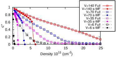
Figure 3: Condensate fraction for the conduction band as a function of the electron and hole density for the same systems as in Fig. 2.

To summarize we have derived a new gap equation for bilayer excitonic systems which includes an effective treatment of the frequency dependence of the electron-hole interaction. The frequency dependence has a dramatic effect on the superfluid gap, which is enhanced substantially and survives at much higher densities. Contrary to the usual static mean-field treatment our results qualitatively agree with both to QMC simulations for simplified systems López Ríos et al. (2018) and experimental measurements for real systems Burg et al. (2018). Our method therefore provides an important complement to existing methods to describe bilayer excitonic systems. For double bilayer graphene at zero magnetic field our calculations predict non-vanishing superfluid gaps across the entire BEC-BCS crossover. Double bilayer graphene may therefore provide a convenient solid-state systems that can be used to investigate the new emerging physics in the crossover regime as well as to design new devices. Contrary to static mean-field calculations we predict that the superfluid gaps are substantial even for small band gaps ($<10$ meV) and that Josephson-like transfer of pairs can be substantial.