Evaluating uncertainties in electrochemical impedance spectra of solid oxide fuel cells

Abstract

Electrochemical impedance spectroscopy (EIS) is a widely used tool for characterization of fuel cells and other electrochemical conversion systems. When applied to the on-line monitoring in the context of in-field applications, the disturbances, drifts and sensor noise may cause severe distortions in the evaluated spectra, especially in the low-frequency part. Failure to ignore the random effects can result in misinterpreted spectra and, consequently, in misleading diagnostic reasoning. This fact has not been often addressed in the research so far. In this paper, we propose an approach to the quantification of the spectral uncertainty, which relies on evaluating the uncertainty of the equivalent circuit model (ECM). We apply the computationally efficient variational Bayes (VB) method and compare the quality of the results with those obtained with the Markov chain Monte Carlo (MCMC) algorithm. Namely, MCMC algorithm returns accurate distributions of the estimated model parameters, while VB approach provides the approximate distributions. By using simulated and real data we show that approximate results provided by VB approach, although slightly over-optimistic, are still close to the more realistic MCMC estimates. A great advantage of the VB method for online monitoring is low computational load, which is several orders of magnitude lower compared to MCMC. The performance of VB algorithm is demonstrated on a case of ECM parameters estimation in a 6 cell solid oxide fuel cell (SOFC) stack. The complete numerical implementation for recreating the results can be found at https://repo.ijs.si/lznidaric/variational-bayes-supplementary-material.

1 Introduction

Currently available tools for characterising electrochemical energy systems predominantly rely on Nyquist curves obtained through electrochemical impedance spectroscopy (EIS) [1]. Conceptually simple and well understood, EIS analysis has become a standard tool for characterising the health condition of cells and stacks. Correct evaluation of the EIS characteristic is subject to several requirements.

First, the perturbation signal must have low amplitude in order not to excite the nonlinear modes of the cells dynamics. If the amplitudes are too small, there is a risk that the noise-to-signal ratio will decrease, which will reflect in an increased variance of the EIS estimates. Second, the cells should operate in stationary, stable, and repeatable test conditions. This is mandatory for a correct evaluation of the EIS curves. The internal conditions should remain constant during the perturbation session and no external disturbance should corrupt the measurements. Under stable laboratory conditions, the effect of disturbances on stack are minimised, which usually results in smooth Nyquist curves. Correctly evaluated EIS spectra ensures accurate detection of fault and stack degradation. Detection is done by checking their similarity to the reference EIS spectra obtained in the healthy state. An anomaly in the online spectra might be ascribed to the fault instead to the disturbances, which results in false fault alarm. Third, to obtain comparable results, measurements on a cell or a stack should be performed at the same operating point. The above requirements are not easily met in applications outside laboratories.

In the in-field operation, the presence of disturbances in the balance of plant (BoP) and system environment is likely to come into play. In the laboratory conditions there are opportunities to apply expensive instrumentation (e.g. on-line gas analyser), high-performance actuators, power electronics and measurement devices. In commercial applications, a trade-off between performance and cost of implementation should normally be sought. Cost optimization dictates reduction of the number and types of implemented sensors to minimum and use of standard industrial modules for HW realisation. Variations in gas channel, drift and noise in flows and temperatures can affect the low-frequency part of the Nyquist curve and can lead to non-smooth results. Increased noise in current and voltage measurements can also contribute to the non-smooth EIS evaluation. In addition, improper operating conditions, such as increased fuel utilization, can cause dispersed values of impedance in the low-frequency part of the spectra. The reason is the local fuel starvation, which then affects the voltage variance.

A strong motivation for the work stems on one hand from experience with some cases of practical implementations and, on the other hand, by the fact that it has not been explicitly addressed in the literature. For better illustration, Figure 1 shows two sets of evaluated EIS curves obtained from successive measurements. The first set was obtained on a short solid oxide fuel cell (SOFC) stack consisting of six planar anode-supported cells installed in an electrical furnace. The stack was operated in the laboratory conditions under nominal current of 32 $\mathrm{A}$ and FU=77.5 %. More details can be found in [2]. The second case is an example of a commercial stack with anode-supported cells operated at around $750^{o}$C and at the power $1$kW. As fuel, natural gas is used in a way that it is first partly transformed to syngas by steam reforming. During the long-term run there were occasional issues related to the periodic component in the fuel and steam flow, which was attributed to the control system issues. Note that perturbations do not significantly affect the high frequency range arcs in the EIS curve.

It seems the problem is relevant for the SOFC systems domain. With the increasing need for automated condition monitoring, robust solutions are mandatory to ensure reliable diagnosis. This is important since the mitigation actions are taken based on the diagnostic results. Unreliable EIS evaluations can result in misleading diagnosis and countermeasures that can even worsen the condition of a cell or a stack.

An idea of how to deal with the problem in SOFCs was recently proposed in articles [3, 4]. The authors perform inference on the equivalent circuit model (ECM) based on a combination of EIS data smoothing and EIS averaging. Instead of using a single EIS measurement, the data from several consecutive EIS measurements are averaged to reduce the dispersion of the EIS estimates in the low-frequency region. This solution, while simple, requires a certain number of measurements spanned on a time window to reliably assess the change in EIS characteristic.

In this paper, we propose a novel approach, not pursued before, which is able to account for the influence of perturbations on the evaluated EIS characteristic, and consequently on the equivalent circuit model, by a statistical modelling approach. Properly quantified uncertainties lead to diagnostic solutions that, rather than making a fault statement in clear yes/no categories, suggest the probability that a particular fault is present [5]. This is essential for cautious and more reliable diagnosis of SOFCs, which can be additionally enhanced with the operator’s prior knowledge.

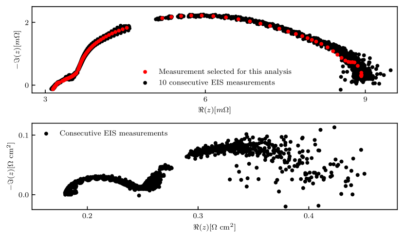
Figure 1: Evaluated EIS characteristics in laboratory conditions (above) and during an in-field application (below).

In the area of electrochemical energy conversion systems, there have been only limited attempts to analyze the stochastic nature of the parameters. Since parameters of the ECM model are usually obtained by constrained nonlinear optimization, the uncertainty of the estimated parameters is obtained from the local properties of the objective function around the optimal parameters, c.f. [6, 7]. The problem with the approach is that the approximation is rather rough and might suggest a misleading uncertainty region [8]. To obtain a realistic estimate of the parameters uncertainty, more elaborated approaches should be applied. Of the available methods, the Markov chain Monte Carlo (MCMC) [9] provides the most accurate probability distributions for estimated model parameters. The key problem with the approach is the overwhelming computational time, which increases rapidly with the number of unknown parameters. That renders the approach inappropriate for in-field on-line condition monitoring. Instead, a computationally less excessive but still sufficiently accurate method is desired.

A remedy for the issues imposed by MCMC is the variational Bayes (VB) [10]. Unlike the MCMC algorithm that results in the “true” posterior distribution, the VB approach provides the closest approximation of the posterior distribution using the probability distribution functions from the family of exponential functions. Consequently, instead of solving the typically intractable evidence integral in pure Bayesian approach, the posterior distribution in VB algorithm is found by means of optimization. The result contains inherent bias, which is a low price to pay considering the impressive computational efficiency of the approach even for multidimensional cases. VB approach has been extensively applied in various areas, such as Gaussian process modeling [11, 12], deep generative models [13], compressed sensing [14, 15], Hidden Markov models [16, 17], reinforcement learning and control [18]. VB approach is also applicable to energy management problems [19, 20, 21, 22, 23].

In this paper we analyse the nature of the uncertainty regions for the ECM parameters and compare the results of the computationally feasible VB approach with the results of MCMC approach. To the best of the authors’ knowledge, the first and only attempt to study the uncertainty of ECM estimates has been done in [24]. That work is the first report on the probability distribution functions of the ECM parameters under nominal operating conditions. Unfortunately, the method is infeasible for on-line monitoring since it takes several hours even with a strong HPC infrastructure. For example, 25 hours are needed to obtain the correct distributions of parameters for the experimental measurement presented later on. What we suggest below is to approximate the true posterior probability density function with a closed form distribution that best captures the nature of the true posterior. The benefits of having the uncertainties of the model parameters explained in the closed form are twofold. First, we get a useful indicator of the quality of the selected ECM model structure and the quality of the experimental data leading to the model. Second, it becomes possible to rather easily employ statistical reasoning tools for detecting changes in the ECM parameters and thus the deterioration of the system behaviour. That is the first such approach in the domain of SOFC.

The organisation of the paper is as follows. A brief introduction to the MCMC and VB approach is given in section 2. The performance of the method in terms of computational efficiency and accuracy is first demonstrated on a simulated ECM in section 3. Finally, the VB algorithm is applied to the identification of ECM parameters based on data obtained on a SOFC in section 4. The main body of the paper is followed by 3 appendices. In A the complete numerical implementation for recreating the results is described. Additional results on VB on simulated measurements with varying degrees of noise can be found in B. Finally, some results of the VB approach on experimental measurements under different conditions are delivered in C.

2 Methodology

Assume we want to describe a process with a model $\mathcal{M}_{\bm{\theta}}$ parameterized by a vector $\bm{\theta}$. Based on measurements $\bm{\mathbf{x}}$ obtained from the process, one would like to get the unknown $\bm{\theta}$ from $\bm{\mathbf{x}}$. Assume also there is some prior knowledge (or guess) about $\bm{\theta}$ expressed in terms of a probability distribution (also called prior distribution ) $p(\bm{\theta})$. Prior knowledge can be updated (improved) with information contained in the data by means of Bayes rule. The result is the posterior distribution $p(\bm{\theta}|\bm{\mathbf{x}})$ as follows

$$\underbrace{p(\bm{\theta}|\mathbf{x})}_{\text{Posterior}}=\frac{\overbrace{p(\mathbf{x}|\bm{\theta})}^{\text{Likelihood}}\overbrace{p(\bm{\theta})}^{\text{Prior}}}{\underbrace{p(\mathbf{x})}_{\text{Evidence}}}$$ (1)

The likelihood can be calculated from the model and the prior is specified as a design input. The normalisation factor (evidence) is the following integral:

$$p(\mathbf{x})=\int_{\bm{\theta}}p(\mathbf{x}|\bm{\theta})p(\bm{\theta})d\bm{\theta}.$$ (2)

For general multidimensional distributions the integral (2) becomes intractable. Consequently, getting the posterior in (1) becomes infeasible, hence the need for the apximate approaches.

2.1 Markov Chain Monte Carlo

MCMC algorithm is a ubiquitous method for solving integration problems (2) in various areas, e.g. statistics, physics and econometrics. Central in the approach is the way of taking samples, say a set of $N$ samples $\bm{\theta}^{(i)}\in\mathbb{R}^{m},\ i=1,...,N$, from a target density $p(\bm{\theta})$. Using these $N$ samples, we can approximate $p(\bm{\theta})$, by calculating the empirical point-mass function

$$p_{N}(\bm{\theta})=\frac{1}{N}\sum_{i=1}^{N}\delta_{\bm{\theta}^{(i)}}(\bm{\theta}),$$

where $\bm{\theta}^{(i)}$ is the $i^{th}$ sample in our set $\mathbf{\theta}$ and $\delta_{\bm{\theta}^{(i)}}$ is its delta-Dirac mass.

In our case we used MCMC with No-U-Turn sampling (NUTS) [25], implemented in Python with the PyMC3 [26] library. NUTS sampling is an extension of the well known Hamiltonian Monte Carlo algorithm (HMC) [27]. HMC tends to be sensitive to the required user inputs. This is mostly avoided since the NUTS algorithm stops automatically when it starts retracing its steps. Additionally, authors of the NUTS developed a method for automatic adaptation of the step size, so that the sampler needs minimal user-defined parameters on entry. For the experimental data described later on, we have let the algorithm run for $300.000$ iterations, which proved sufficient to guarantee convergence.

2.2 Variational Bayes

Using MCMC methods for solving (2) can produce results very close to the true posterior distribution. However, for the multidimensional cases, the computational load and sheer number of samples required for obtaining proper estimate of the posterior blows up. One solution to this problem is to find a sufficiently close approximation of the posterior with the significantly lower computational load.

The main idea of the VB approach is finding a candidate distribution $q_{\bm{\lambda}}(\bm{\theta})$ (parameterized with the hyperparameters $\bm{\lambda}\in\mathbb{R}^{\nu}$), that is a sufficiently close approximation of the true posterior $p(\bm{\theta}|\mathbf{x})$. The distribution $q_{\bm{\lambda}}(\bm{\theta})$ is usually referred to as the variational distribution. The variational distribution is typically selected from the mean-field variational family [28]. This means that one can assume independence among the latent variables of the variational distribution.

A variational distribution that is the best fit for the true posterior can be obtained by minimizing the Kullback-Leibler (KL) divergence [28], which can be re-arranged as follows:

$$\begin{split}\lx@glossaries@gls@link{acronym}{kl}{\leavevmode KL}(q_{\bm{\lambda}}(\bm{\theta})||p(\bm{\theta}|\mathbf{x}))&=\mathbb{E}_{q}\left[\log\frac{q_{\bm{\lambda}}(\bm{\theta})}{p(\bm{\theta}|\mathbf{x})}\right]\\ &=\mathbb{E}_{q}[\log q_{\bm{\lambda}}(\bm{\theta})]-\mathbb{E}_{q}[\log p(\bm{\theta}|\mathbf{x})]\\ &=\mathbb{E}_{q}[\log q_{\bm{\lambda}}(\bm{\theta})]-\mathbb{E}_{q}[\log p(\mathbf{x},\bm{\theta})-\log p(\mathbf{x})]\\ &=\mathbb{E}_{q}[\log q_{\bm{\lambda}}(\bm{\theta})]-\mathbb{E}_{q}[\log p(\bm{\theta},\mathbf{x})]+\log p(\mathbf{x})\\ &=-({\mathbb{E}_{q}[\log p(\bm{\theta},\mathbf{x})]-\mathbb{E}_{q}[\log q_{\bm{\lambda}}(\bm{\theta})]}+\log p(\mathbf{x})\\ &=-\underbrace{(\mathbb{E}_{q}[\log p(\mathbf{x}|\bm{\theta})p(\bm{\theta})]-\mathbb{E}_{q}[\log q_{\bm{\lambda}}(\bm{\theta})])}_{L(\bm{\lambda},\bm{x})}+\log p(\mathbf{x})\end{split}$$ (3)

Second term $\log p(\mathbf{x})$ is constant. The first term $L(\bm{\lambda})$is known as evidence lower bound (ELBO) and by maximising it one can minimize the KL divergence between the variational distribution and the true posterior. So the goal is to solve the following optimization problem:

$$\bm{\lambda}^{*}=\underset{\bm{\lambda}\in\Omega}{\arg\min}\lx@glossaries@gls@link{acronym}{kl}{\leavevmode KL}(q_{\bm{\lambda}}(\bm{\theta})||p(\bm{\theta}|\mathbf{x}))=\underset{\bm{\lambda}\in\Omega}{\arg\max}{L(\bm{\lambda},\bm{x})},$$ (4)

where ${\Omega}$ is the set of all possible values of the hyperparameters $\bm{\lambda}$. The overall idea is schematically presented in Figure 2. It is assumed that the model parameters are random variables. However, their true distribution is almost always unknown. In such a case, the best option is to select an approximate candidate distribution that will be used instead. When selecting the candidate distribution, we try to incorporate prior knowledge as much as possible, in particular the support interval, previous empirical observations, etc. Some mismatch between the selected distributions and true posterior is usually always present, which causes a bias in the VB solution. However, this is a small price to pay compared to the substantial increase in the computational efficiency of the VB approach. The VB algorithm was implemented in Python using the PyTorch [29] library. For a link to the implementation and an example data set sufficient to recreate a numerical example, see A.

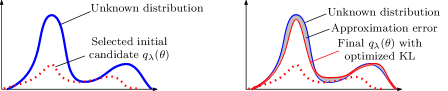
Figure 2: Optimization process of finding the closest variational distribution $q_{\bm{\lambda}}(\bm{\theta})$ over the set of latent variables $\bm{\lambda}$.

2.3 Finding the optimal hyper-parameters

Using VB we convert the problem of finding the posterior distributions from statistical inference to a much simpler task of optimizing a cost function for a variational family parameterised by the vector of hyperparameters $\bm{\lambda}$. The cost function in this case is ELBO. For the optimization part of our algorithm we use the adaptive moment estimation (ADAM) optimizer [30].

ADAM allows an adaptive correction of the learning rates for each element $\lambda^{(s)},s=1,...,\nu$ of the vector $\bm{\lambda}$ during the run of the algorithm by calculating the first and second moment of the gradient, denoted as ${m}_{t}^{(s)}$ and $v_{t}^{(s)}$ respectively. This is done using exponentially moving averages computed on the gradient $g_{t}^{(s)},\ s=1,...,\nu$

$$\begin{split}m_{t}^{(s)}&=\beta_{1}m_{t-1}^{(s)}+(1-\beta_{1})g_{t}^{(s)}\\ v_{t}^{(s)}&=\beta_{2}v_{t-1}^{(s)}+(1-\beta_{2})\left(g_{t}^{(s)}\right)^{2},\end{split}$$ (5)

where $t$ denotes the iteration number and $\beta_{1,2}$ are the parameters of the moving average. The default values for $\beta$ parameters are 0.9 and 0.999 and the initial values of first and second moment of the gradient are both set to $0$, since it turns out this does not impact the convergence rate significantly. For a set of measured data (impedance in our case) $\bm{x}$, the gradients can be presented with the following vector

$$\bm{g}_{t}=\left(g_{t}^{(1)},\ldots,g_{t}^{(\nu)}\right)^{T}=\nabla_{\bm{\lambda}_{t}}L(\bm{\lambda}_{t},\bm{x}).$$ (6)

The first and the second moment are only estimated with $m^{(s)}$ and $v^{(s)}$, therefore we want them to satisfy the following condition

$$\begin{split}\mathbb{E}\{m_{t}^{(s)}\}&=\mathbb{E}\left(g_{t}^{(s)}\right)\\ \mathbb{E}\{v_{t}^{(s)}\}&=\mathbb{E}\left((g^{(s)}_{t})^{2}\right)\end{split}$$ (7)

Above conditions ensure that we are dealing with unbiased estimates. First moment at step $t$ in the recursive equation (5) is

$$m_{t}^{(s)}=\left(1-\beta_{1}\right)\sum_{i=1}^{t}\beta_{1}^{t-i}{g}_{i}^{(s)}.$$ (8)

We can see some bias still occurs in this estimate. Applying expected value operator to equation (8) gives us

$$\begin{split}E_{\lambda}\left[m_{t}^{(s)}\right]&=\left(1-\beta_{1}\right)\sum_{i=1}^{t}\beta_{1}^{t-1}E_{\lambda}\left[{g}_{i}^{(s)}\right]\\ &\approx\left(1-\beta_{1}\right)\left(\sum_{i=1}^{t}\beta_{1}^{t-1}\right)E_{\lambda}\left[{g}_{t}^{(s)}\right]\\ &=\left(1-\beta_{1}^{t}\right)E_{\bm{\lambda}}\left[{g}_{t}^{(s)}\right].\end{split}$$ (9)

Bias correction is done automatically by ADAM during the evaluation of $m$ and $v$ as follows

$$\begin{split}\hat{m}_{t}^{(s)}&=\frac{m_{t}^{(s)}}{1-\beta_{2}^{t}}\\ \hat{v}_{t}^{(s)}&=\frac{v_{t}^{(s)}}{1-\beta_{2}^{t}}.\end{split}$$ (10)

Optimization steps are also adjusted. For each individual parameter the algorithm updates

$$\lambda_{t}^{(s)}=\lambda_{t-1}^{(s)}-\eta\frac{\hat{m}_{t}^{(s)}}{\sqrt{\hat{v}_{t}^{(s)}}+\eta},$$ (11)

where $\eta=0.001$.

The use of ADAM is widely used across many areas and applications since it delivers efficient and fast results. It should be noted, however, that as a heuristic optimization algorithm there is no general guarantee for convergence. Fortunately, Kingma and Ba [30] proved that the algorithm converges globally in the convex settings. This was further refined and proved by Reddi et al. [31]. We used the default settings of $\beta_{1}=0.9$ and $\beta_{2}=0.999$, while setting the learning rate depending on the data set at hand. The number of iterations is at least $8000$ but no more than $35000$. An additional stopping criterion was defined by converged ELBO values, i.e. when the relative change of less than $1\%$ is achieved over $1000$ iterations. In all of the optimization runs the maximum number of iterations were almost never reached. The average number of iterations was around $13000$.

3 Numerical example

Since we focus on solid oxide fuel cells in this paper, we will first demonstrate the performance of VB algorithm using simulated data. The rationale for the model structure arises from the electrochemical arguments explained in more detail in section 4. The model can be represented as a serial connection of resistance, inductance and RQ elements

$$Z(\omega)=R_{s}+\sum_{i=1}^{N}\frac{R_{i}}{(j\omega)^{\alpha_{i}}Q_{i}R_{i}+1}+j\omega L$$ (12)

where $R_{s}$ stands for serial resistance, $R_{i}$ is parallel resistance and $Q_{i}$ constant-phase parameter, fractional order of $i^{th}$ pole is denoted with $\alpha_{i}\in(0,1]$, $\omega=2\pi f$ and $f$ is frequency. The schematic of the ECM structure is given in Figure 3. For the simulation study below we take $N=3$.

Figure 3: The ECM as a series of RQ-elements.

The “true” impedance (12) was simulated on the frequency interval $f\in[10^{-4},10^{4}]$ Hz by using parameters listed in Table 1. The additive measurement noise was applied separately to the voltage $u(t)$ and current $i(t)$ as $n_{1}(t)$ and $n_{2}(t)$ respectively. It should be noted that $n_{1}(t)$ and $n_{2}(t)$ are zero-mean and uncorrelated. Having the simulated input and output signals, the transfer function was estimated from Morlet wavelet transform of the input and output as described in [32]. The entire process is presented in Figure 4.

Figure 4: Simulation of EIS data with additive noise in input and output.

Table 1: Model parameters and variational distributions calculated using equations (13) and (14).

True parameter	Variational distribution
$R_{s}$ = $3$ $\Omega$	$\sim\text{Lognormal}(0.84,0.39)$
$R_{1}=1$ $\Omega$, $R_{2}=2$ $\Omega$, $R_{3}=3$ $\Omega$	$\sim\text{Lognormal}(1.59,0.20)$
$Q_{1}=0.1$ $Fs^{\alpha_{1}}$	$\sim\text{Lognormal}(-0.35,0.83)$
$Q_{2}=5$ $Fs^{\alpha_{2}}$	$\sim\text{Lognormal}(1.96,0.83)$
$Q_{3}=150$ $Fs^{\alpha_{3}}$	$\sim\text{Lognormal}(4.99,0.55)$
$\alpha_{1}=0.88$, $\alpha_{2}=0.82$, $\alpha_{3}=0.99$	$\sim\text{Beta}(13.91,5.68)$
$L=100~{}nH$

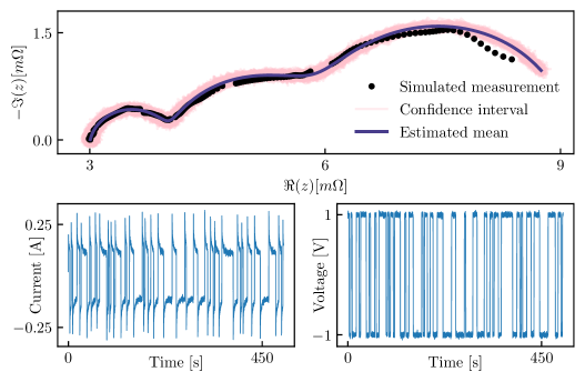
Figure 5: Results of the VB algorithm (above). Current and voltage signals used in simulation (below).

The first step in applying the VB approach is the definition of variational distributions that approximate the true posterior $p(\bm{\theta}|\mathbf{x})$. They are listed in Table 1. For our case $\bm{\theta}\in\mathbb{R}_{+}^{10}$, with additional limitation as $\alpha_{i}\in[0,1]$ . Beta distribution was therefore chosen as the best fit for the $\alpha_{i},i\in\{1,2,3\}$ parameters and Log-normal distribution for the rest. We selected the means and variances for our variational distributions and then determined their parameters using (13) and (14).

Rough estimates of variational distributions can be assessed from the EIS curve in Figure 5, previous experience and integrating experts knowledge. In the upper plot in Figure 5 one can notice that the real part of the curve starts around $3$ $\Omega$. This provides a rough estimate for the parameter $R_{s}$. Hence selecting variational distribution with mean $2.5$ $\Omega$ and variance to $1$ seems a reasonable choice. The next step is setting up the variational distributions for the parameters $R_{1,2,3}$. Just by looking at the axis values, it is apparent that they should be located within the interval (1,10) $\Omega$. Mean values of their distributions were therefore set in the middle of the interval. Variational distributions of the parameters $Q_{1,2,3}$ were roughly estimated with the help of experiences gained from previous experiments and by incorporating experts knowledge. Lastly, the fractional order powers $\alpha_{1,2,3}$ are expected to have values in the interval [0.5,1] so we set their variational distributions with means at $0.75$.

Once we have determined the mean and variance of our variational distributions, we have to transform them into the correct parameters for the chosen distributions. To obtain the parameters of the log-normal distribution $(\sigma_{ln},\mu_{ln})$ from the mean and variance $(\sigma,\mu)$, the following equations can be used:

$$\sigma_{ln}=\ln\left(\frac{\sigma^{2}}{\sqrt{\sigma^{2}+\mu^{2}}}\right)\hskip 56.9055pt\mu_{ln}=\ln\left(1+\frac{\mu^{2}}{\sigma^{2}}\right)$$ (13)

and for beta distribution parameters $\alpha$ and $\beta$ e.g. $\text{Beta}(\alpha,\beta)$ we use:

$$\alpha=\frac{\sigma^{2}-\sigma^{3}}{\mu}-\sigma\hskip 56.9055pt\beta=\frac{\alpha}{\sigma}-\alpha$$ (14)

The optimization was performed using a global learning rate of $0.05$ and was completed after $25000$ steps. ELBO loss curve can be observed in Figure 6. By sampling the resulting posterior distributions and simulating the model (12) it is possible to visualize the obtained results. For this purpose, $1000$ samples were drawn for each parameter from their respective posterior distribution. Simulating the $1000$ EIS curves with the sampled sets of parameters gave us an estimate of the confidence interval of our results, which can be found in Figure 5. The EIS curve obtained from the means of the posterior distributions for the parameters can also be found on the same Figure. The variance of the posterior distributions is effectively presented with the sampled curves and it is bound by the noise variance parameter. The mean EIS curve seems to be a sufficiently good fit for the input data.

Additional results demonstrating the performance of the VB algorithm on simulated data with heavy additive noise can be found in B.

Figure 6: The evolution of ELBO loss during optimization process.

The evolution of the optimization process for each parameter is presented in Figure 7, where we can also find the true parameters used for the simulation of our input data. We can see that each parameter reaches its true value, except $Q_{3}$. We can assume this is the effect of noise, which seems to be greater in the third arc, as seen in Figure 5. Progress in confidence of the algorithm can be easily observed with the help of the evolution of estimated spread in parameter distributions. As seen in the Figure 7, the spread is wide at the beginning and as the optimization progresses and explores larger search space it steadily narrows.

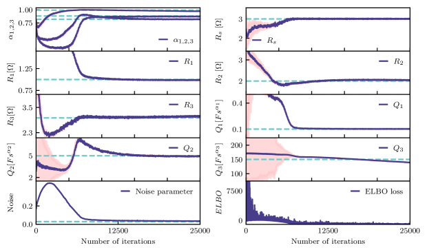
Figure 7: Progress of parameter estimation during the optimization process, true values of parameters used for simulation are represented with dashed lines. The variance of the estimated distribution(pink) is quite low. The selected optimal shape of the posterior distributions are shown in Figure 8.

The resulting posterior distributions of the model parameters as well as the posteriors obtained with MCMC are shown in Figure 8. Three key observations can be made. First, comparing posterior and variational distributions, the optimization process was capable of reaching the “true” mean values even for cases when the variational means were “far” from the simulated values. Second, the scales (variance) of the posterior distributions are low, leading to the conclusion that the obtained model has low uncertainty. Table 2 lists all the resulting posterior parameter distributions. Third, the empirical posteriors obtained through MCMC method are similar to the ones obtained by VB approach. It should be noted that in some cases VB posteriors can be under-dispersed (lower variance) compared to the ones obtained by MCMC. Being overconfident is a well known behavioural trait of VB algorithm and a mathematical proof of this behaviour under certain conditions is provided by Blei and Wang [8, 33]. Our results seem to fit the MCMC results reasonably well, with minor overconfidence in the posterior distributions of $R_{1,2}$ and $Q_{3}$.

Table 2: Posterior distributions of parameters.

$R_{s}\sim\text{Lognormal}(1.0,0.0006)$
$R_{1}\sim\text{Lognormal}(-0.011,0.003)$	$R_{2}\sim\text{Lognormal}(0.72,0.002)$	$R_{3}\sim\text{Lognormal}(1.12,0.003)$
$Q_{1}\sim\text{Lognormal}(-2.28,0.0007)$	$Q_{2}\sim\text{Lognormal}(1.6,0.007)$	$Q_{3}\sim\text{Lognormal}(4.94,0.004)$
$\alpha_{1}\sim\text{Beta}(969.35,144.11)$	$\alpha_{2}\sim\text{Beta}(1016.18,225.57)$	$\alpha_{3}\sim\text{Beta}(4724.72,144.39)$

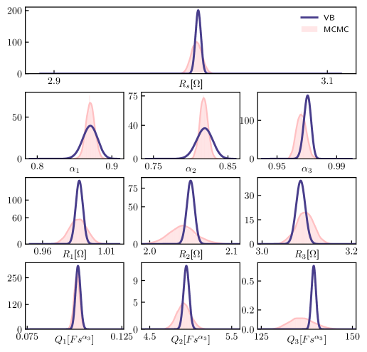
Figure 8: Posterior distributions of parameters derived from simulated data.

4 Experimental validation

The VB was validated using EIS curves measured on stack of $6$ anode supported solid oxide fuel cells which were installed in an insulated ceramic housing. Stack operated for a total of 4500 hours at the operating temperature of $750$ °C. The active area of a single cell was 80 cm². The SOFC short stack was fed with a mixture of hydrogen and nitrogen with a flow rate H2/N2=0.216/0.144 Nl h^-1cm^-2 whereas the air flow rate was 4 Nl h^-1cm^-2. Stack was operated at nominal current of 32 $\mathrm{A}$ (0.4 $\mathrm{A}\text{\,}{\mathrm{cm}}^{-2}$) with fuel utilization of 77.5 %.

The EIS curves were obtained by current excitation (galvanostatic mode) with discrete random binary signal. The excitation current had DC value of I${{}_{\text{DC}}}$=32 A with peak-to-peak amplitude of 2 A. The amplitude was chosen low to ensure linearised stack response, but still large enough to guarantee sufficient signal-to-noise ratio.

The current and voltage sensor have sufficiently wide frequency bandwidth with cut-off frequency of 240 kHz. The cell voltages were measured independently using a differential 16-bit NI USB-6215 data acquisition system. The analogue signals were firstly low pass filtered at 10.8 kHz and sampled with sampling frequency $f_{s}=50$ kHz. Additional information about the SOFC short stack in question can be found in [2].

4.1 Experimental results

The measured EIS curve is shown in Figure 10. Note here that the noise in measurements is quite low thanks to the high-quality data acquisition equipment and the well controlled laboratory conditions for the experiment.

The first step in model identification is the selection of the model structure. In our case that breaks down to the selection of $N$, the number of RQ elements and to do so physical arguments are used. In case of hydrogen as a fuel one could expect five dominant processes divided into three main groups [34]: gas conversion, cathode processes and anode processes. Their time constants span the frequency band from 0.1 Hz to 1 Mhz. The gas conversion processes are related to the low frequency part of the EIS curve, the cathode processes are mainly visible in the mid-frequency range and the high-frequency part can be attributed to the anode related processes. The contribution of each group can be seen in Figure 9.

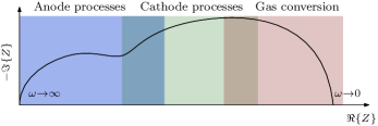
Figure 9: Main groups of processes within the hydrogen-powered SOFC.

Variational distributions were selected by examining the measured EIS curve. If we look at the Figure 10, we can see that the high frequency part of the real component has values around $3\text{m}\Omega$, which will serve as the mean value for the $R_{s}$ parameter. The scale of its distribution was set quite large to allow the optimization process to explore broad intervals in the search for the optimum. Variational distributions of $R_{1,2,3}$ parameters can be inferred from the complex and real values our EIS curve takes that their values should be roughly between the interval [0.1,3] m$\Omega$. From previous testing and by incorporating experts knowledge we can assume that the $Q_{1,2,3}$ parameters will be at least by an order of $10$ apart, so we assumed they are located at $1,50$ and $500$ $Fs^{\alpha_{1}}$ respectively. The scales for their variational distributions were set respectively large. Finally, for $\alpha_{1,2,3}$ we can assume from experience that they probably take values between $0.5$ and $1.0$, therefore the means of their variational distributions were set at $0.75$. All the variational distributions can be seen on Table 3.

Table 3: Variational distributions of parameters used for estimation of parameters for experimental data.

$R_{s}\sim\text{Lognormal}(-5.86,0.32)$	$R_{1,2,3}\sim\text{Lognormal}(-8.41,1.27)$	$\alpha_{1,2,3}\sim\text{Beta}(12,3)$
$Q_{1}\sim\text{Lognormal}(-2.31,2.14)$	$Q_{2}\sim\text{Lognormal}(3.57,0.83)$	$Q_{3}\sim\text{Lognormal}(6.20,0.20)$

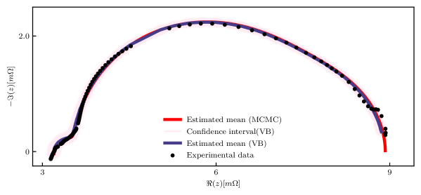
Figure 10: Measured EIS and the estimated mean EIS values from MCMC and VB.

The learning rate was set to $0.005$. This value is lower than in the numerical example, since the goal was to allow steady and efficient estimation. The optimization finished after $35000$ steps.

The performance of the algorithm can best be observed by looking at the EIS curves obtained from the posterior distributions of the estimated parameters. In the same manner as with numerical example, we also took $1000$ samples from each of parameters posterior distribution, to simulate $1000$ EIS curves. The confidence interval is shown in Figure 10, together with the EIS curve obtained from the posterior means. The results confirm that despite the low number of iterations, the resulting parameters represent an accurate fit for the measured EIS data.

The convergence of ELBO can be seen in Figure 11. Comparing with the Figure 6 we can notice that the rate of convergence is slower, which can be associated with the much smaller learning rate and smaller number of iterations used for the run on experimental data. As optimization approaches the end, the ELBO value changes minimally, which means the optimal estimates have been found.

Figure 11: The evolution of ELBO for experimental data.

The evolution of parameter estimation is shown in Figure 13. The algorithm steadily converges towards the optimum, while the estimated spread for each parameter continues to decrease. The parameter evolution is very smooth for each parameter. Posterior distributions are shown in Figure 14, where we compare them with results of MCMC algorithm. We can see the expected slight overconfidence of VB, while the results are still inline with MCMC results. It is apparent that scales (variance) of the posterior distributions are quite low. Posterior parameter distributions are listed in Table 4.

Additional VB approach results on different settings for SOFC can be found in C, including a result on a measurement recorded after a leakage fault has occured.

Table 4: Posterior distributions of the parameters.

$R_{s}\sim\text{Lognormal}(-5.75,8.3e^{-4})$
$R_{1}\sim\text{Lognormal}(-7.995,0.011)$	$R_{2}\sim\text{Lognormal}(-6.33,0.0039)$	$R_{3}\sim\text{Lognormal}(-5.61,0.0075)$
$Q_{1}\sim\text{Lognormal}(2.25,0.0086)$	$Q_{2}\sim\text{Lognormal}(6.22,0.0025)$	$Q_{3}\sim\text{Lognormal}(3.96,0.0028)$
$\alpha_{1}\sim\text{Beta}(1081.56,41.42)$	$\alpha_{2}\sim\text{Beta}(2216.36,187.46)$	$\alpha_{3}\sim\text{Beta}(399.28,0.495)$

4.2 Comparison of Variational Bayes with averaging spectra

Averaging the EIS obtained from successive measurements is a pragmatic way to reduce the effects of measurement noise. The more spectra are averaged, the better the filtration of noise is. However, in practice that means many repeated perturbations are needed.

Using VB approach, we can compute a comparable result by using only one measurement. For the comparison, we averaged 10 consecutive measured spectra and compared with the results of the VB approach on the last among them.

The results are presented in Figure 12, where measured EIS data are in the upper part, while the mean estimate from VB approach and the evaluated average are presented in the lower part. The results of both methods are very similar, even though the VB approach used information from only one measurement. That is practical benefit in the context of online health monitoring.

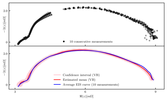
Figure 12: Comparison of VB approach and averaging EIS spectra. Ten consecutive EIS evaluations are used (upper part). The compared VB posterior and averaged spectra are on the lower graph.

4.3 Discussion

Results in Figure 10 that the ECM identified through the VB approach provide an accurate fit for the measured data.

From ELBO plot in Figure 11 it is evident the algorithm converges. The same observation holds true for the estimated parameters, as shown in Figure 13.

Comparing the resulting posterior distributions from both VB and MCMC in Figure 14 we can conclude the following. First, results show close match for every parameter, with only a slight mismatch noticeable in $R_{s},\alpha_{1}$ and $Q_{1}$. Second, the posterior distributions obtained with VB have lower dispersion (variance) than the ones obtained through MCMC. As mentioned above, this is common for VB approach.

One of the reasons for having overconfident results might be in the selection of the variational distributions. A possible improvement might be achieved by using more elaborated approximations in terms of a mixture of bounded distributions [35]. That is a topic of further research.

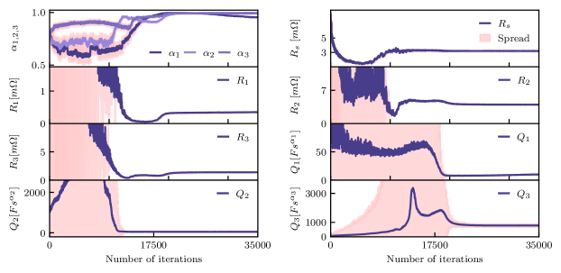
Figure 13: The evolution of the parameter estimates for experimental data.

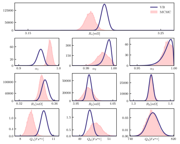
Figure 14: Posterior distributions of parameters inferred from experimental data by VB and MCMC algorithm.

5 Conclusion

In this paper a novel approach to the statistical estimation of the ECM parameters of SOFC impedance spectra is presented. From a single EIS evaluation, the approach is able to evaluate the uncertainty in the model parameters caused by noise and disturbances in the system. The VB approach was validated on simulated data as well as on experimental measurements.

The simulation reveals that even in the case of excessive degree of noise the VB algorithm still produces accurate estimates. Main benefit of using the method is low computational load when compared to the commonly used MCMC approach. In particular, to obtain comparable results the time needed was approximately 5 minutes for VB approach and around 25 hours for MCMC on the same computational power. Validation tests indicate that the difference in performance between two methods is minimal, which renders VB as an option for on-line SOFC monitoring.

Full information on the estimated value and accompanying uncertainty helps avoid misinterpretation of the EIS data corrupted by noise and disturbances. It is shown that the results of VB might be comparable with the results obtained by averaging the spectra. The key advantage of VB is that only one evaluated EIS is needed to get the information for which several spectra in the averaging approach are needed (more spectra means more stack perturbation).

The future work will concentrate on the design of the detection approach that fully exploits the information provided by the VB. It is expected that evaluated uncertainties in the estimated parameters will result in a more cautious diagnosis, which will be insensitive to the illogical shapes of the impedance characteristics.

Appendix A Supplementary material: numerical implementation

​​​​ ​​​​ Supplementary material containing numerical implementation of the VB algorithm can be found at https://repo.ijs.si/lznidaric/variational-bayes-supplementary-material​​. Python Jupyter notebook file SupplementaryMaterialSVI.ipynb contains the main algorithm. Data set used to recreate the results presented in this article can be found in NumPy file dataset.npz. Repository contains all the needed scripts for implementation of VB algorithm. Simulation of data was however done separately, so the code is not included.

Appendix B Additional results on simulated measurements

Additional simulation runs with the model from section 3 are performed under different noise levels in current and voltage. Noise $n_{1}(t)$ and $n_{2}(t)$ was added both to the voltage $u(t)$ as well as current $i(t)$ respectively. It should be noted that $n_{1}(t)$ and $n_{2}(t)$ are zero-mean and uncorrelated. Most interesting results were selected and are presented here. Table 5 contains the information about selected measurements. The results suggest that even in the case of high noise level the VB produces plausible estimate of the true EIS characteristic.

Table 5: Noise levels used in simulation.

Measurement number	$1$	$2$	$3$
Input noise	$\mathcal{N}(0.0,0.0)$	$\mathcal{N}(0.0,0.00005)$	$\mathcal{N}(0.0,0.05)$
Output noise	$\mathcal{N}(0,0.0)$	$\mathcal{N}(0,0.001)$	$\mathcal{N}(0,0.05)$

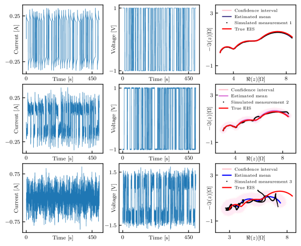
Figure 15: Simulated current, voltage and the resulting EIS curves with different noise settings along with VB estimated mean and the confidence region.

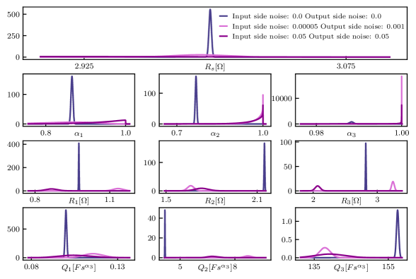
Figure 16: Posterior parameter distributions obtained by VB approach on simulated noisy data. Uncertainty in the parameters increases with increasing level of noise used for simulation.

Appendix C Additional results on experimental measurements

The method was tested on a set of measured EIS data at different currents in healthy state and on data under leakage fault. Measurement presented in the main article is obtained during the nominal running conditions of the SOFC which are 77% fuel utilization and current of 32 A. Main operating conditions of additional measurements are presented in Table 6. Measurement 1 and Measurement 2 are obtained during different fuel utilization settings. For Measurement 1, fuel utilization was increased from 77% to 72% by decreasing the gas flow and keeping the current steady at  32 A. On the flip side, fuel utilization in Measurement 2 was increased from 72% to 87% by increasing the electrical current from  32 A to 36.4 A. Measurement 3 was recorded after a leakage fault occured in the plant. In Figure 17 the results of VB algorithm are presented. The VB algorithm returns good estimates for each of the measurement, irrespective of the fact that the same set of variational distributions are applied. The resulting posterior distributions for each parameter are presented in Figure 18.

Table 6: Operational conditions for the measurements.

Measurement number	$1$	$2$	$3$
Current [A]	$32.21$	$36.39$	$32.04$
Fuel utilization [$\%$]	$82$	$87$	$77$

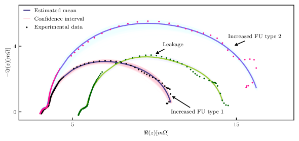
Figure 17: VB results for 3 EIS measurements at different operational conditions.

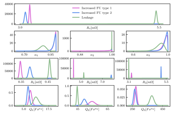
Figure 18: Posterior distributions of ECM parameters obtained on 3 measurements under different conditions explained in Table 6.

References

- Lasia [2014] A. Lasia, Electrochemical Impedance Spectroscopy and its Applications, Springer-Verlag, New York, 2014.
- Nusev et al. [2021] G. Nusev, B. Morel, J. Mougin, Đ. Juričić, P. Boškoski, Condition monitoring of solid oxide fuel cells by fast electrochemical impedance spectroscopy: A case example of detecting deficiencies in fuel supply, Journal of Power Sources 489 (2021) 229491. URL: https://www.sciencedirect.com/science/article/pii/S0378775321000409. doi:https://doi.org/10.1016/j.jpowsour.2021.229491.
- Mougin et al. [2019] J. Mougin, B. Morel, A. Ploner, P. Caliandro, J. Van Herle, P. Boškoski, B. Dolenc, M. Gallo, P. Polverino, A. Pohjoranta, A. Nieminen, S. Pofahl, J. Ouweltjes, S. Diethelm, A. Leonardi, F. Galiano, C. Tanzi, Monitoring and diagnostics of sofc stacks and systems, ECS Transactions 91 (2019) 731–743. doi:10.1149/09101.0731ecst.
- Gallo et al. [2020] M. Gallo, P. Polverino, J. Mougin, B. Morel, C. Pianese, Coupling electrochemical impedance spectroscopy and model-based aging estimation for solid oxide fuel cell stacks lifetime prediction, Applied Energy 279 (2020) 115718. URL: http://www.sciencedirect.com/science/article/pii/S0306261920312113. doi:https://doi.org/10.1016/j.apenergy.2020.115718.
- Rakar et al. [1999] A. Rakar, Đ. Juričić, P. Ballé, Transferable belief model in fault diagnosis, Engineering Applications of Artificial Intelligence 12 (1999) 555 – 567. URL: http://www.sciencedirect.com/science/article/pii/S0952197699000305. doi:https://doi.org/10.1016/S0952-1976(99)00030-5.
- Mosbæk [2014] R. Mosbæk, Solid Oxide Fuel Cell Stack Diagnostics, Ph.D. thesis, 2014.
- Leonide [2010] A. Leonide, SOFC Modelling and Parameter Identification by Means of Impedance Spectroscopy, Schriften des Instituts für Werkstoffe der Elektrotechnik, Karlsruher Institut für Technologie, KIT Scientific Publ., 2010. URL: https://books.google.si/books?id=kE3Otpn2DS8C.
- Wang and Blei [2019] Y. Wang, D. M. Blei, Variational Bayes under model misspecification, 2019. arXiv:1905.10859.
- Jacob et al. [2018] P. E. Jacob, S. M. M. Alavi, A. Mahdi, S. J. Payne, D. A. Howey, Bayesian inference in non-markovian state-space models with applications to battery fractional-order systems, IEEE Transactions on Control Systems Technology 26 (2018) 497–506.
- Šmídl and Quinn [2006] V. Šmídl, A. Quinn, The Variational Bayes Method in Signal Processing, Springer-Verlag, 2006. doi:10.1007/3-540-28820-1.
- Bui et al. [2016] T. D. Bui, J. Yan, R. E. Turner, A unifying framework for Gaussian process pseudo-point approximations using power expectation propagation (2016). arXiv:1605.07066v3.
- Hensman et al. [2014] J. Hensman, A. Matthews, Z. Ghahramani, Scalable variational Gaussian process classification (2014). arXiv:1411.2005v1.
- Rezende et al. [2014] D. J. Rezende, S. Mohamed, D. Wierstra, Stochastic backpropagation and approximate inference in deep generative models (2014). arXiv:1401.4082v3.
- Yang et al. [2012] Z. Yang, L. Xie, C. Zhang, Variational Bayesian algorithm for quantized compressed sensing (2012). doi:10.1109/TSP.2013.2256901. arXiv:1203.4870v2.
- Oikonomou et al. [2019] V. P. Oikonomou, S. Nikolopoulos, I. Kompatsiaris, A novel compressive sensing scheme under the variational Bayesian framework, IEEE, 2019, pp. 1–5. doi:10.23919/EUSIPCO.2019.8902704.
- Gruhl and Sick [2016] C. Gruhl, B. Sick, Variational Bayesian inference for hidden markov models with multivariate Gaussian output distributions (2016). arXiv:1605.08618v1.
- Panousis et al. [2020] K. P. Panousis, S. Chatzis, S. Theodoridis, Variational conditional-dependence hidden markov models for human action recognition (2020). arXiv:2002.05809v1.
- Levine [2018] S. Levine, Reinforcement learning and control as probabilistic inference: Tutorial and review (2018). arXiv:1805.00909v3.
- Liu et al. [2020] Y. Liu, H. Qin, Z. Zhang, S. Pei, Z. Jiang, Z. Feng, J. Zhou, Probabilistic spatiotemporal wind speed forecasting based on a variational Bayesian deep learning model, Applied Energy 260 (2020) 114259. doi:10.1016/j.apenergy.2019.114259.
- Liu et al. [2019] Y. Liu, H. Qin, Z. Zhang, S. Pei, C. Wang, X. Yu, Z. Jiang, J. Zhou, Ensemble spatiotemporal forecasting of solar irradiation using variational Bayesian convolutional gate recurrent unit network, Applied Energy 253 (2019) 113596. doi:10.1016/j.apenergy.2019.113596.
- Choi et al. [2018a] W. Choi, H. Kikumoto, R. Choudhary, R. Ooka, Bayesian inference for thermal response test parameter estimation and uncertainty assessment, Applied Energy 209 (2018a) 306–321. doi:10.1016/j.apenergy.2017.10.034.
- Choi et al. [2018b] W. Choi, K. Menberg, H. Kikumoto, Y. Heo, R. Choudhary, R. Ooka, Bayesian inference of structural error in inverse models of thermal response tests, Applied Energy 228 (2018b) 1473–1485. doi:10.1016/j.apenergy.2018.06.147.
- Pasquier and Marcotte [2020] P. Pasquier, D. Marcotte, Robust identification of volumetric heat capacity and analysis of thermal response tests by Bayesian inference with correlated residuals, Applied Energy 261 (2020) 114394. doi:10.1016/j.apenergy.2019.114394.
- Dolenc et al. [2020] B. Dolenc, G. Nusev, P. Boškoski, B. Morel, J. Mougin, Đ. Juričić, Probabilistic deconvolution of solid oxide fuel cell impedance spectra, 2020. doi:10.1007/978-3-030-37161-6.
- Hoffman and Gelman [2011] M. D. Hoffman, A. Gelman, The no-u-turn sampler: Adaptively setting path lengths in hamiltonian Monte Carlo (2011). arXiv:1111.4246.
- Salvatier et al. [2016] J. Salvatier, T. V. Wiecki, C. Fonnesbeck, Probabilistic programming in python using PyMC3, PeerJ Computer Science 2 (2016) e55. URL: https://doi.org/10.7717/peerj-cs.55. doi:10.7717/peerj-cs.55.
- Betancourt [2017] M. Betancourt, A conceptual introduction to Hamiltonian Monte Carlo (2017). arXiv:1701.02434.
- Blei et al. [2016] D. M. Blei, A. Kucukelbir, J. D. McAuliffe, Variational inference: A review for statisticians (2016). doi:10.1080/01621459.2017.1285773. arXiv:1601.00670v9.
- Paszke et al. [2019] A. Paszke, S. Gross, F. Massa, A. Lerer, J. Bradbury, G. Chanan, T. Killeen, Z. Lin, N. Gimelshein, L. Antiga, A. Desmaison, A. Kopf, E. Yang, Z. DeVito, M. Raison, A. Tejani, S. Chilamkurthy, B. Steiner, L. Fang, J. Bai, S. Chintala, Pytorch: An imperative style, high-performance deep learning library, in: H. Wallach, H. Larochelle, A. Beygelzimer, F. d'Alché-Buc, E. Fox, R. Garnett (Eds.), Advances in Neural Information Processing Systems 32, Curran Associates, Inc., 2019, pp. 8024–8035. URL: http://papers.neurips.cc/paper/9015-pytorch-an-imperative-style-high-performance-deep-learning-library.pdf.
- Kingma and Ba [2014] D. P. Kingma, J. Ba, Adam: A method for stochastic optimization, 2014. arXiv:1412.6980.
- Reddi et al. [2019] S. J. Reddi, S. Kale, S. Kumar, On the convergence of adam and beyond (2019). arXiv:1904.09237v1.
- Boškoski et al. [2017] P. Boškoski, A. Debenjak, B. M. Boshkoska, Fast Electrochemical Impedance Spectroscopy, Springer International Publishing, 2017. doi:10.1007/978-3-319-53390-2.
- Wang and Blei [2018] Y. Wang, D. M. Blei, Frequentist consistency of variational Bayes, Journal of the American Statistical Association 114 (2018) 1147–1161. URL: http://dx.doi.org/10.1080/01621459.2018.1473776. doi:10.1080/01621459.2018.1473776.
- Lang et al. [2008] M. Lang, C. Auer, A. Eismann, P. Szabo, N. Wagner, Investigation of solid oxide fuel cell short stacks for mobile applications by electrochemical impedance spectroscopy, Electrochimica Acta 53 (2008) 7509–7513. URL: https://www.sciencedirect.com/science/article/pii/S0013468608004982. doi:https://doi.org/10.1016/j.electacta.2008.04.047, 7th International Symposium on Electrochemical Impedance Spectroscopy.
- Tenreiro [2013] C. Tenreiro, Boundary kernels for distribution function estimation, REVSTAT Statistical Journal 11 (2013) 169–190.