Long term X-Ray Observations of Seyfert 1 Galaxy Ark 120: On the origin of soft-excess

Abstract

We present the long-term X-ray spectral and temporal analysis of a ‘bare-type AGN’ Ark 120. We consider the observations from XMM-Newton, Suzaku, Swift, and NuSTAR from 2003 to 2018. The spectral properties of this source are studied using various phenomenological and physical models present in the literature. We report (a) the variations of several physical parameters, such as the temperature and optical depth of the electron cloud, the size of the Compton cloud, and accretion rate for the last fifteen years. The spectral variations are explained from the change in the accretion dynamics; (b) the X-ray time delay between 0.2-2 keV and 3-10 keV light-curves exhibited zero-delay in 2003, positive delay of $4.71\pm 2.1$ ks in 2013, and negative delay of $4.15\pm 1.5$ ks in 2014. The delays are explained considering Comptonization, reflection, and light-crossing time; (c) the long term intrinsic luminosities, obtained using nthcomp, of the soft-excess and the primary continuum show a correlation with a Pearson Correlation Co-efficient of $0.922$. This indicates that the soft-excess and the primary continuum are originated from the same physical process. From a physical model fitting, we infer that the soft excess for Ark 120 could be due to a small number of scatterings in the Compton cloud. Using Monte-Carlo simulations, we show that indeed the spectra corresponding to fewer scatterings could provide a steeper soft-excess power-law in the 0.2-3 keV range. Simulated luminosities are found to be in agreement with the observed values.

1 Introduction

Active Galactic Nuclei (AGNs) are the most energetic phenomena in the universe. The emitted radiation is observed over the entire range of the electromagnetic spectrum. The high energy X-rays are believed to be emitted from the innermost region of an accretion disc which surrounds the central black hole (Shakura & Sunyaev, 1973; Pringle et al., 1973). The X-ray spectra of Seyfert 1 galaxies, a subclass of AGNs, is mostly fitted by a power-law component with photon index in the range $\Gamma=1.6-2.2$ (Bianchi et al., 2009; Sobolewska & Papadakis, 2009) and a high energy cut-off. The spectral contribution which deviates from the power-law at lower energy (below $\sim 2$ keV) is known as ‘soft excess’ (Halpern, 1984; Arnaud et al., 1985; Singh et al., 1985). The X-ray spectra are often associated with a Fe K$\alpha$ line, which is observed near 6.4 keV, and a Compton hump in the energy range of 20.0 to 40.0 keV. It has been observed that the primary power-law emission is produced by the Comptonization of low energy seed photons (Sunyaev & Titarchuk, 1980; Titarchuk, 1994) emitted from the standard Keplerian disc. The seed photons are processed from the accretion mechanism, and the peak emission arises at optical/ultraviolet (UV) wavelengths (Pringle et al., 1973) for a supermassive black hole (SMBH). However, the location, as well as the geometry of the Compton reprocessing region, are still a matter of debate. This Compton cloud can be situated above the accretion disc (Haardt & Maraschi, 1991, 1993; Poutanen & Svensson, 1996) or at the base of the relativistic jet (Chakrabarti & Titarchuk, 1995; Fender et al., 1999, 2004; Markoff et al., 2005). The region could be a hot, radiatively inefficient and behave like a quasi-Bondi flow as discussed initially by Ichimaru (1977). This region could originate the thermal Comptonization of soft photons produced in the optical/UV range from an optically thick Keplerian disc (Magdziarz et al., 1998; Dewangan et al., 2007; Done et al., 2012; Lohfink et al., 2012) or a blurred reflection from ionized disc (Fabian et al., 2002; Ross & Fabian, 2005; Crummy et al., 2006; García et al., 2014). The iron line is thought to be originated by the photoelectric absorption followed by the fluorescence line emission from a dense and relatively cold accretion disc. Moreover, it is believed that the Compton hump could be due to the Compton scattering dominated above 10 keV in a relatively cold dense medium. Nevertheless, the complex broad-band spectrum of AGNs requires a proper physical explanation of the flow dynamics and radiative properties around the central engine across the soft and hard energy regime of the X-ray.

In this scenario, the Two-Component Advective Flow (TCAF) (Chakrabarti & Titarchuk, 1995) model, which combines the essence of all the salient features of a viscous transonic flow (Chakrabarti, 1989, 1990, 1995) around black holes is worth exploring. It is a physical solution encompassing hydrodynamics and radiative processes. The transonic flow solution allows two types of accretion flows depending on how efficiently angular momentum is being transported: a viscous, geometrically thin, optically thick standard Keplerian component (Shakura & Sunyaev, 1973) and a weakly viscous, geometrically thick, optically thin sub-Keplerian halo component (Chakrabarti & Titarchuk, 1995). The latter is basically an inefficiently radiating generalized Bondi flow with high radial velocity till it forms the centrifugal barrier after which it becomes efficient in radiating at higher energies. The Keplerian disc is formally truncated at the centrifugal barrier, the outer boundary of which is the shock location (Chakrabarti, 1989). The post-shock region (i.e., the region between the shock and the innermost sonic point) is known as CENtrifugal barrier supported BOundary Layer or CENBOL and it acts as the Compton cloud. The soft photons from the Keplerian disc are upscattered by Comptonization process in the post-shock region and produce the high energy X-ray photons. TCAF, a self-consistent model, is quantified by four flow parameters: two types of accretion rates, namely, the disc rate ($\dot{m}_{d}$) and halo rate ($\dot{m}_{h}$), size and density of the Compton cloud, through the shock location ($X_{s}$) and the compression ratio ($R$), ratio of the post-shock and the pre-shock flow densities ($\frac{\rho_{+}}{\rho_{-}}$). It also requires an intrinsic parameter, namely, the mass of the central black hole (in the units of $M_{\odot}$), and an extrinsic parameter, namely, the normalization which is required to place the observed spectrum over the theoretical spectrum of TCAF. The broadband spectra of M87 was explained with this model by fitting the data from multi-wavelength observations(Mandal & Chakrabarti, 2008). Later, TCAF has been implemented in the xspec as a local table model and has been successful to fit the data of the Galactic black holes (Debnath et al., 2014) and has also been able to estimate the mass of nearby Seyfert 1 galaxy NGC 4151 using NuSTAR data (Nandi et al., 2019).

Arakelian 120 (Ark 120) is a nearby ($z=0.03271$) radio-quiet Seyfert 1 AGN with radio-loudness $R\approx 0.1$ (Condon et al., 1998; Ho, 2002). This source was intensely monitored nearly in all wavelengths: optical/UV (Kollatschny et al., 1981, 1981; Schulz & Rafanelli, 1981; Alloin et al., 1988; Marziani et al., 1992; Peterson et al., 1998; Stanic et al., 2000; Popović et al., 2001; Doroshenko et al., 2008; Kuehn et al., 2008) and X-ray (Vaughan et al., 2004; Nardini et al., 2016; Reeves et al., 2016; Gliozzi et al., 2017; Lobban et al., 2018) and was found to be consistently bright in optical, UV, and X-rays displaying substantial wavelength-dependent variability (Gliozzi et al., 2017; Lobban et al., 2018). From the simultaneous UV/X-ray measurements, it was reported that the observations are neither ‘contaminated’ by absorption signatures along the line of sight (Vaughan et al., 2004; Reeves et al., 2016; Crenshaw et al., 1999) nor by neutral intrinsic absorbers (Reeves et al., 2016) around the central engine. Furthermore, Ark 120 is nearly free from intrinsic reddening in the IR-optical-UV continuum (Ward et al., 1987; Vasudevan et al., 2009). Therefore, it provides one of the cleanest views ($N_{H}\sim 3\times 10^{19}$ cm^-2; (Vaughan et al., 2004)) of the central region. This type of AGNs are called “bare nucleus” Seyferts or bare AGNs. The estimated mass of the central black hole of Ark 120 is M${}_{BH}=1.50\pm 0.19\times 10^{8}$ M_⊙ (Peterson et al., 2004) which was measured using the reverberation-mapping technique. From the spectroscopic monitoring data of Ark 120 during 1976 to 2013 using a 70 cm telescope, Denissyuk et al. (2015) estimated the mass of the central SMBH to be M${}_{BH}=1.675\pm 0.028\times 10^{8}$ M_⊙. This source has a low Eddington ratio of $L_{bol}/L_{E}\sim 0.05$ (Vasudevan & Fabian, 2007) with a strong soft-excess (Matt et al., 2014; Porquet et al., 2004, 2019) and a significant broad Fe K_α line (Vaughan et al., 2004; Nardini et al., 2011). Nardini et al. (2011) analyzed Ark 120 spectra, where, in the absence of absorber of complex morphology, soft-excess was explained by reflection from the centrally located hot and cold medium located at a distance. Marinucci et al. (2019) used the Monte-Carlo technique to investigate the favourable shape of the Compton cloud considering the future polarimetric missions such as IXPE (Weisskopf et al., 2016).

Although Ark 120 is a widely studied source, the evolution of the X-ray spectra over the last two decades is yet to be understood. However, a steepening of the X-ray spectrum was observed during six-month monitoring in 2014 with Swift. The observed spectral variability was attributed to the possible existence of a large disc reprocessing region (Gliozzi et al., 2017). Again during 2017-18, a longer time delay was observed (Lobban et al., 2018) between longer wavelength difference (i.e., optical and X-ray). They predicted that the accretion disc could exist in a longer scale as predicted by standard accretion disc theory. The soft-excess part of Ark 120 could be originated due to the Comptonization within the hot electron cloud of various shape (Marinucci et al., 2019), reflection from a cold medium (Nardini et al., 2011) or the shock heating near the inner edge of the disc (Fukumura et al., 2016). We analyzed the long term X-ray archival data of Ark 120 which provides an ideal testbed to understand the soft-excess as well as its interaction with the harder (>2 keV) photons. Along with the observations, we perform Monte-Carlo simulations to find the effect of Comptonizaton within the energy range of soft-excess. We also study the X-ray variability of the source over a longer period and to calculate the approximate time-delays in X-ray bands. For the first time, we also find the flow and system parameters by fitting of the X-ray data. The paper is structured in the following way: in Sec 2, we provide the details of the observational data and their reduction procedure. The results of the spectral and temporal analysis are presented in Sec 3 and 4. We discuss our findings in Sec 5 and finally, draw our conclusions in Sec 6.

2 Observation and Data Reduction

We use the publicly available archival data of XMM-Newton, NuSTAR, Chandra, and Suzaku using HEASARC. We reprocessed all data using HEAsoft v6.26.1 (Arnaud, 1996), which includes XSPEC v12.10.1f.

Table 1: Observation Log

ID	Date	Obs. ID	Instrument	Exposures
	(yyyy-mm-dd)			(ks)
XMM1	2003-08-24	0147190101	XMM-Newton/EPIC-pn	112.15
S1	2007-04-01	702014010	Suzaku/XIS-HXD	100.86
XRT1	2008-07-24	00037593001	Swift/XRT	10.86
	-2008-08-03	-00037593003
XMM2	2013-02-18	0693781501	XMM-Newton/EPIC-pn	130.46
N1	2013-02-18	60001044004	NuSTAR/FPMA	65.46
XMM3	2014-03-22	0721600401	XMM-Newton/EPIC-pn	124.0
N2	2014-03-22	60001044002	NuSTAR/FPMA	55.33
XRT2	2014-09-04	00091909002	Swift/XRT	22.81
	-2014-10-19	-00091909022
XRT3	2014-10-22	00091909023	Swift/XRT	20.18
	-2014-12-05	-00091909044
XRT4	2014-12-09	00091909045	Swift/XRT	23.48
	-2015-01-26	-00091909068
XRT5	2015-01-26	00091909069	Swift/XRT	21.66
	-2015-03-15	-00091909090
XRT6	2017-12-07	00010379001	Swift/XRT	44.14
	-2018-01-24	-00010379048

2.1 XMM-Newton

Ark 120 has been observed by XMM-Newton (Jansen et al., 2001) during three epochs from 2003 to 2014. In 2003 and 2013, it has made $\sim$ 112 ks (XMM1) and $\sim$ 130 ks (XMM2) observations respectively. The XMM1 data is used by (Vaughan et al., 2004) and reported that the source Ark 120 is one of the cleanest Sy1 type AGN. In 2014, XMM-Newton observed Ark 120 four times between March 18 and March 24. Out of these, one (XMM3) was simultaneous with NuSTAR observation. The details of the observation log are presented in Table  1. It was observed that the X-ray flux of this source was about a factor of two higher in 2014 than the XMM2 observation (Matt et al., 2014; Marinucci et al., 2019) made in 2013. A similar trend of flux variation was also reported in optical/UV (Lobban et al., 2018) band.

Due to the high brightness of the source, the European Photon Imaging Camera (EPIC-pn (Strüder et al., 2001)) operated in Small Window (SW) mode to prevent any pile-up. The details of the XMM-Newton/EPIC-pn observations of this source are listed in Table-1. We reprocessed the raw data to level 1 data for EPIC-pn by Scientific Analysis System (SAS v16.1.0) with calibration files dated February 2, 2018. We have used only the unflagged (FLAG == 0) events for excluding the edge of CCD and the edge of the bad pixel. Besides this, we also use PATTERN $\leq 4$ for single and double pixel. We exclude the photon flares by proper GTI files to acquire the maximum signal to noise ratio. After that, we use an annular area of 30″  outer radii and 5″  inner radii centered at the source to extract the source event. For the background, we use a circle of 60″  in the lower part of the window that contains no (or negligible) source photons. The response files (arf and rmf files) for each EPIC-pn spectral data set were produced with SAS tasks ARFGEN and RMFGEN, respectively. The GRPPHA task is used with 100 counts per bin for 0.3 - 10.0 keV EPIC-pn spectra.

2.2 Suzaku

Suzaku observed Ark 120 on 2007 April 1 (Obs ID: 702014010) in HXD normal position with exposure of $\sim$ 101 ks using X-ray imaging spectrometer (Koyama et al., 2007) and $\sim$ 89 ks for Hard X-ray Detector (Takahashi et al., 2007). The photons were collected in both $3\times 3$ and $5\times 5$ editing modes. From this observation, a presence of soft-excess emission in soft X-ray was reported by (Nardini et al., 2011). Also, Fe K$\alpha$ emission line with full-width at half maximum of $4700^{+2700}_{-1500}$ km s^-1 was previously reported by (Nardini et al., 2016) by using Suzaku observation along with XMM-Newton, Chandrai, and NuSTAR.

We use the standard data reduction technique for Suzaku data analysis illustrated in Suzaku Data Reduction Guide and followed the recommended screening criteria while extracting Suzaku/XIS spectrum and light-curves. The latest calibration files available (2014-02-03) using FTOOLS 6.25 is used to reprocess the event files. The source spectra and lightcurves are extracted from a circular region of radius 200″centered on the Ark 120 and the background region is selected on the same slit with a circular region 250″. Finally, we merge the two front illuminated detectors (XIS0 and XIS3) to produce the final spectra and lightcurves for Ark 120. We generated the response files through XISRESP script.

As Suzaku has a high energy X-ray detector (HXD), we use the HXD/PIN data for our analysis. We reprocessed the unfiltered event files using the standard tools. The output spectrum and lightcurves are extracted by using the hxdpinxbpi and hxdpinxblc, respectively. Further, we correct the spectrum to take into account both the non-X-ray and the cosmic X-ray backgrounds and the dead time correction.

2.3 NuSTAR

NuSTAR (Harrison et al., 2013) observed Ark 120 simultaneously with XMM-Newton with FPMA and FPMB on 2013 February 18 (N1) and 2014 March 22 (N2) for the exposure of $\sim$166 ks and $\sim$ 131 ks respectively. The details of the observation log are given in Table  1. We consider both N1 and N2 observations for our analysis. (Porquet et al., 2018, 2019) used this data along with XMM-Newton and determined the spin $0.83^{+0.05}_{-0.03}$ and comment on the dimension of the corona and temperature by analyzing these X-ray data.

The level 1 data is produced from the raw data by using the NuSTAR data analysis software (NuSTARDAS v1.8.0). The cleaned event files are produced with standard NUPIPELINE task and calibrated with the latest calibration files available in the NuSTAR calibration database (CALDB). We chose 90″  radii for source and 180″  radii for the background region on the same detector to avoid contamination and detector edges. For the final background-subtracted lightcurves, we use 100s bin for both FPMA and FPMB. As both detectors are identical, here we present the results of FPMA only. The response files (arf and rmf files) are generated by using the numkrmf and numkarf modules, respectively.

2.4 Swift data

Swift X-ray telescope (XRT; Burrows et al. (2005)), working in the energy range of 0.2 to 10.0 keV, is an X-ray focusing telescope. XRT observed this source in both WT (windowed timing) and pc (photon count) modes depending on the brightness of the source. Ark 120 was observed over $\sim 130$ times from 2008-07-24 to 2018-01-24. In 2008, Swift observed three times, July 24, July 31 and August 3. We stack the spectra to produce a combined spectrum (XRT1). Then, it again observed on 2014-03-22, which has a simultaneous observation with XMM and NuSTAR. We consider the XMM3 observation over this particular XRT observation. Swift observed Ark 120 from 2014-09-06 to 2015-03-15 on a nearly daily basis. Further, we stack these observations into four observations (XRT2, XRT3, XRT4, XRT5) with each observations spanning around 50 days. In the last epoch, Swift observed Ark 120 from 2017-12-05 to 24-01-2018 over $\sim$ 50 days. We stack the observations to produce the spectra of XRT6. The details of the observation log are stated in Table 1. We use the online tool “XRT product builder” Evans et al. (2009) to extract the spectrum and light curves. This product builder performs all necessary processing and calibration and produces the final spectra and lightcurves of Ark 120 in WT and PC mode.

3 Spectral Analysis

We use XMM-Newton, Suzaku, NuSTAR, and Swift data for the spectral analysis and explore the spectral variation over $\sim$15 years (2003-2018) period using XSPEC v12.10.1f (Arnaud, 1996). We explore the broad spectral properties with nthcomp model (Zdziarski, Johnson & Magdziarz, 1996). Later, we apply Two Component Advective Flow (TCAF) model (Chakrabarti & Titarchuk, 1995) to extract the physical flow parameters such as the accretion rates and size of the Compton cloud.

Along with these models, we use a Gaussian component for the Fe fluorescent emission line. While fitting the data, we use two absorption components, namely TBabs and zTBabs (Wilms et al., 2000). The component, TBabs is used for the Galactic absorption, where hydrogen column density ($N_{H,gal}$) is fixed at $9.78\times 20^{20}$ cm^-2 (Kalberla et al., 2005). To calculate the error for each parameter in spectral fitting with 90% confidence level, we use ‘error’ command in XSPEC.

We use following cosmological parameters in this work: $H_{0}$ = 70 km s^-1 Mpc ^-1, $\Lambda_{0}$ = 0.73, $\Omega_{M}$ = 0.27 (Bennett et al., 2003). With the assumed cosmological parameters, the luminosity distance of Ark 120 is 142 Mpc.

Table 2: nthcomp fitting result for the spectrum above 3.0 keV. The optical depth $\tau$ is calculated from equation-1.

ID	MJD	$\Gamma^{nth}$	$kT_{e}$	Fe $K_{\alpha}$	EW	$\chi/dof$	$\tau^{*}$
			(keV)	(keV)	(eV)
XMM1	$52875$	$1.90^{+0.01}_{-0.01}$	$159.45^{+81.68}_{-81.69}$	$6.40^{+0.016}_{-0.017}$	$116^{+3}_{-4}$	312.33/300	$0.733\pm 0.003$
S1	$54191$	$2.08^{+0.03}_{-0.03}$	$124.65^{+35.54}_{-35.21}$	$6.38^{+0.052}_{-0.052}$	$710^{+10}_{-10}$	1117.31/1093	$0.726\pm 0.008$
XRT1	$54676$	$1.76^{+0.02}_{-0.08}$	$217.72^{+105.6}_{-112.5}$	-	-	75.68/74	$0.671\pm 0.030$
XMM2+N1	$56341$	$1.75^{+0.01}_{-0.02}$	$221.56^{+105.3}_{-107.5}$	$6.42^{+0.061}_{-0.062}$	$136^{+8}_{-9}$	644.55/641	$0.670\pm 0.074$
XMM3+N2	$56738$	$1.87^{+0.01}_{-0.01}$	$205.95^{+100.6}_{-99.87}$	$6.37^{+0.052}_{-0.052}$	$227^{+12}_{-11}$	508.07/469	$0.612\pm 0.003$
XRT2	$56926$	$1.60^{+0.01}_{-0.02}$	$274.40^{+136.5}_{-130.8}$	$-$	-	306.65/290	$0.700\pm 0.008$
XRT3	$56974$	$1.84^{+0.02}_{-0.02}$	$215.72^{+105.5}_{-105.8}$	$-$	-	319.98/320	$0.610\pm 0.006$
XRT4	$57024$	$1.72^{+0.02}_{-0.03}$	$225.57^{+109.7}_{-109.9}$	$-$	-	269.17/280	$0.688\pm 0.011$
XRT5	$57073$	$1.88^{+0.02}_{-0.02}$	$201.58^{+99.78}_{-99.20}$	$-$	-	246.53/261	$0.616\pm 0.006$
XRT6	$58118$	$1.65^{+0.02}_{-0.02}$	$246.87^{+120.9}_{-122.8}$	$-$	-	327.78/318	$0.708\pm 0.008$

Table 3: Soft-excess spectral indices are generated while keeping the spectral slope of nthcomp ($\Gamma^{nth}$) frozen. Intrinsic luminosities are calculated for both of the components using clum in the energy energy 0.5 to 10.0 kev.

ID	$\Gamma^{PC}$	$Norm^{PC}$	$L^{PC}$	$\Gamma^{SE}$	$Norm^{SE}$	$L^{SE}$
	$=\Gamma^{nth}$	$(10^{-2})$			$(10^{-2})$
XMM1	$1.90$	$1.16^{+0.04}_{-0.05}$	$44.18^{+0.06}_{-0.07}$	$3.15^{+0.07}_{-0.06}$	$0.58^{+0.02}_{-0.02}$	$43.66^{+0.05}_{-0.04}$
S1	$2.08$	$18^{+20.3}_{-25.6}$	$45.35^{+0.05}_{-0.05}$	$2.52^{+0.02}_{-0.02}$	$2105^{+10.6}_{-16.5}$	$45.58^{+0.04}_{-0.04}$
XRT1	$1.76$	$0.66^{+0.03}_{-0.03}$	$43.99^{+0.04}_{-0.04}$	$4.11^{+0.22}_{-0.20}$	$0.84^{+0.10}_{-0.10}$	$43.87^{+0.02}_{-0.03}$
XMM2+N1	$1.75$	$0.57^{+0.03}_{-0.03}$	$43.93^{+0.05}_{-0.05}$	$3.03^{+0.03}_{-0.02}$	$0.19^{+0.03}_{-0.05}$	$43.16^{+0.03}_{-0.03}$
XMM3+N2	$1.86$	$1.21^{+0.01}_{-0.01}$	$44.90^{+0.04}_{-0.04}$	$4.23^{+0.02}_{-0.02}$	$0.88^{+0.10}_{-0.10}$	$43.19^{+0.04}_{-0.04}$
XRT2	$1.60$	$0.48^{+0.03}_{-0.03}$	$44.92^{+0.04}_{-0.04}$	$2.92^{+0.19}_{-0.20}$	$0.57^{+0.03}_{-0.04}$	$43.66^{+0.04}_{-0.04}$
XRT3	$1.84$	$0.79^{+0.03}_{-0.04}$	$44.04^{+0.05}_{-0.05}$	$3.27^{+0.27}_{-0.27}$	$0.47^{+0.06}_{-0.06}$	$43.57^{+0.05}_{-0.05}$
XRT4	$1.72$	$0.57^{+0.04}_{-0.05}$	$43.94^{+0.04}_{-0.04}$	$2.53^{+0.10}_{-0.12}$	$0.39^{+0.05}_{-0.06}$	$43.54^{+0.04}_{-0.04}$
XRT5	$1.88$	$0.76^{+0.03}_{-0.03}$	$44.00^{+0.04}_{-0.04}$	$3.17^{+0.34}_{-0.34}$	$0.31^{+0.05}_{-0.05}$	$43.37^{+0.05}_{-0.05}$
XRT6	$1.65$	$0.42^{+0.02}_{-0.03}$	$43.84^{+0.03}_{-0.03}$	$2.96^{+0.28}_{-0.29}$	$0.23^{+0.02}_{-0.03}$	$43.27^{+0.06}_{-0.05}$

Table 4: The TCAF parameter space is defined in the file lmod.dat.

Model parameters	Parameter units	Default value	Min.	Min.	Max.	Max.	Increment
$\rm M_{BH}$	$\rm M_{Sun}$	$\rm 1.0\times 10^{8}$	$2\times 10^{6}$	$2\times 10^{6}$	$5.5\times 10^{9}$	$5.5\times 10^{9}$	$10.0$
$\dot{m}_{d}$	$\rm Edd$	$\rm 0.001$	$0.0001$	$0.0001$	$1.0$	$2.0$	$0.0001$
$\dot{m}_{h}$	$\rm Edd$	$\rm 0.01$	$0.0001$	$0.0001$	$2.0$	$3.0$	$0.0001$
$\rm X_{s}$	$\rm r_{g}$	$\rm 100.0$	$10.0$	$10.0$	$1000.0$	$1000.0$	$2.0$
$\rm R$		$\rm 1.5$	$1.1$	$1.1$	$6.8$	$6.8$	$0.1$

3.1 Nthcomp

We have started the spectral fitting with nthcomp model, and the model in XSPEC reads as:

TBabs*zTBabs*(nthcomp+zGaussian)

nthcomp is a thermally Comptonized continuum model proposed by Zdziarski, Johnson & Magdziarz (1996) and later extended by Zycki, Done & Smith (1999). We fit all X-ray spectrum above 3.0 keV by this baseline model. The model depends on the seed photon energy ($kT_{bb}$), which we consider at 3 eV for all spectrum. Although, Marinucci et al. (2019) considered $kT_{bb}$ at 15 eV. It is to be noted that, we vary $kT_{bb}$ from 1 eV to 50 eV, and failed to notice any deviation in the residuals of the fitted spectra. We consider these seed photons to be disc-blackbody type. For that, we have opted for the inp-type is 1 for all fit. For the spectral fitting, first, we consider the energy range 3.0 to 10.0 keV. The fitted asymptotic power-law photon index $\Gamma=1.90$, electron temperature $kT_{e}=159.45$ keV and an iron K$\alpha$ line at 6.40 keV with equivalent width (EW) of $116^{+3}_{-4}$ eV with reduced chi-square ($\chi^{2}/dof$)=1.04 for degrees of freedom (dof) = 300 is obtained. Next, we analyse the data from the 2007 Suzaku observation. We have combined the Suzaku/XIS observation with Suzaku/HXD and make a spectrum from 0.5 to 40.0 keV. But, we fit 3.0 to 40.0 keV spectrum using the baseline model. The fitted parameters are $\Gamma=2.08$, $kT_{e}=124.65$ keV and iron K$\alpha$ line at 6.38 keV with equivalent width (EW) of $710^{+10}_{-10}$ eV. We are also in need of an additional powerlaw and Gaussian to take care of high energy (above 10.0 keV) spectrum and emission lines. We have obtained the reduced chi-square ($\chi^{2}/dof$)=1.02 for degrees of freedom (dof) = 1093 for this fitting. We have fitted the combined spectrum of XMM2+N1 (MJD-56341) and XMM3+N2 (MJD-56738) spectrum using this model for the energy range 3.0 to 79.0 keV with the model parameters such as $\Gamma=1.75$ & $1.87$ and corresponding $kT_{e}=221.56$ & $205.95$ respectively. We have applied a zGaussian for a Fe K$\alpha$ line at $6.42^{+0.061}_{-0.062}$ & $6.37^{+0.052}_{-0.052}$ keV with equivalent widths (EW) of $136^{+8}_{-9}$ & $227^{+12}_{-11}$ eV for these combined spectra and the ($\chi^{2}/dof$)=644.55/641 & ($\chi^{2}/dof$)= 508.07/469 respectively. Next, we analyse the data obtained from Swift/XRT observation for the energy range of 3.0 to 10.0 keV. Fe K$\alpha$ line is not detected for all the six XRT spectra. We have fitted the Swift/XRT spectra by removing Gaussian component from the baseline model. The power-law index $\Gamma$ vary from 1.60 to 1.88 and the corresponding electron temperature $kT_{e}$ vary from 274.40 to 201.58 keV respectively. The nthcomp model fitted spectral analysis result is presented in Table 2. Furthermore, we calculate the optical depth for each observation using the formula:

$$\tau=\sqrt{\frac{9}{4}+\frac{3}{\theta_{e}(\Gamma+2)(\Gamma-1)}}-\frac{3}{2},$$ (1)

by inverting the relation A1 is presented in Zdziarski, Johnson & Magdziarz (1996). Here, $\theta_{e}=\frac{kT_{e}}{m_{e}c^{2}}$ is the electron energy with respect to the rest mass energy. The value of optical depth $\tau$ for each observation is provided in Table 2. The maximum error in optical depth is obtained from $\Delta\tau\sim(\frac{1}{2}\frac{\Delta\theta_{e}}{\theta_{e}}+\frac{\Delta\Gamma}{\Gamma})\times\tau$, where $\Delta\theta_{e}$ and $\Delta\Gamma$ are considered from the fitted errors presented in Table 2.

We address the soft-excess (< 3 keV) part by adding another powerlaw component. We freeze the $\Gamma$ obtained earlier while fitting the primary continuum alone. The second power-law fits the soft-excess, and the results are presented in Table 3. It should be noted that the spectral index of soft-excess ($\Gamma^{SE}$) is higher than the spectral index of the primary continuum ($\Gamma^{PC}$) for every observation.

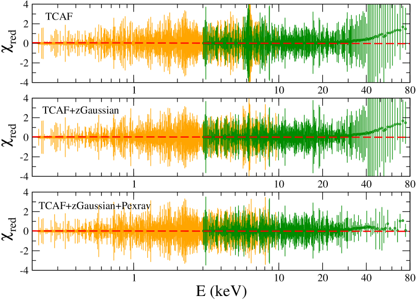
Figure 1: Variation of $\chi_{red}$ is shown for each model components on broadband spectra of Ark 120 during 2014 epoch. Primarily, we have started with TCAF, and then added zGaussian and Pexrav upon necessity.

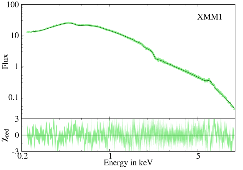
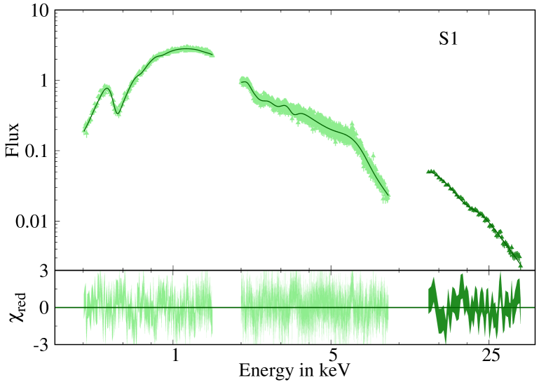
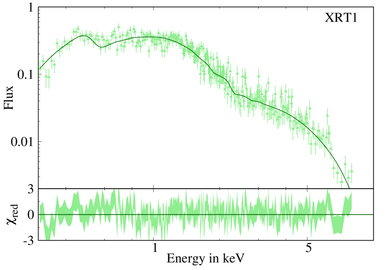
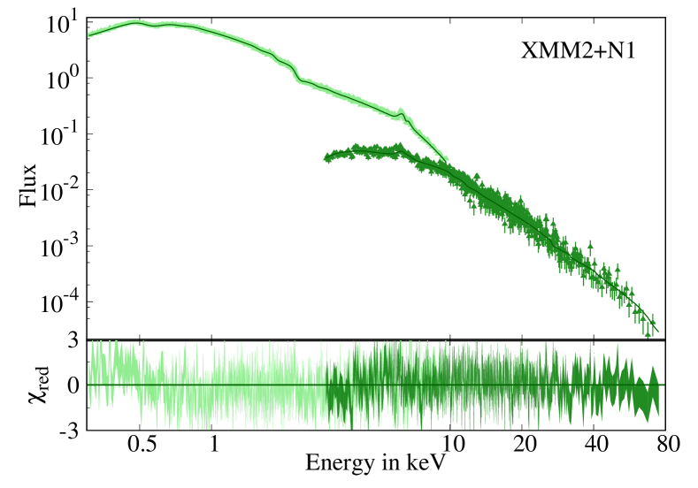
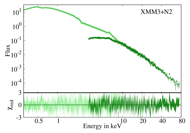
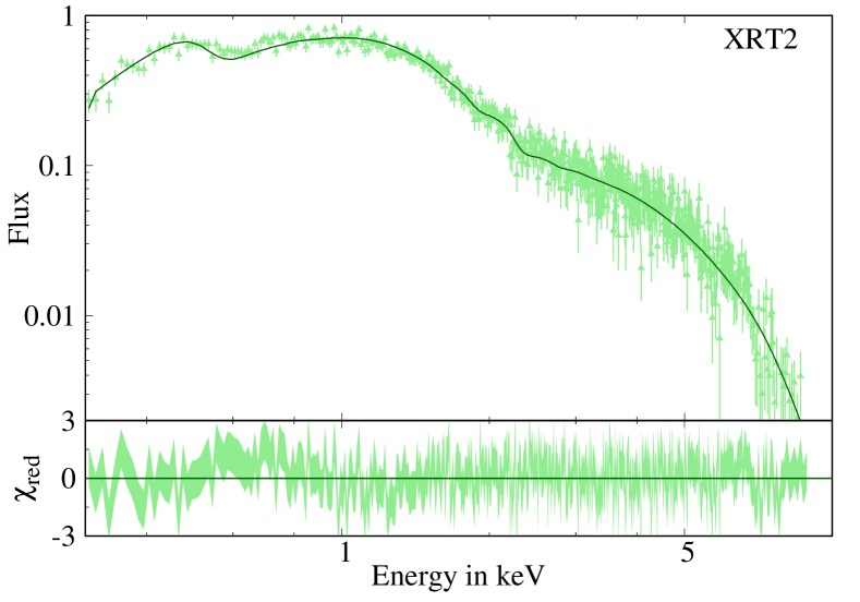
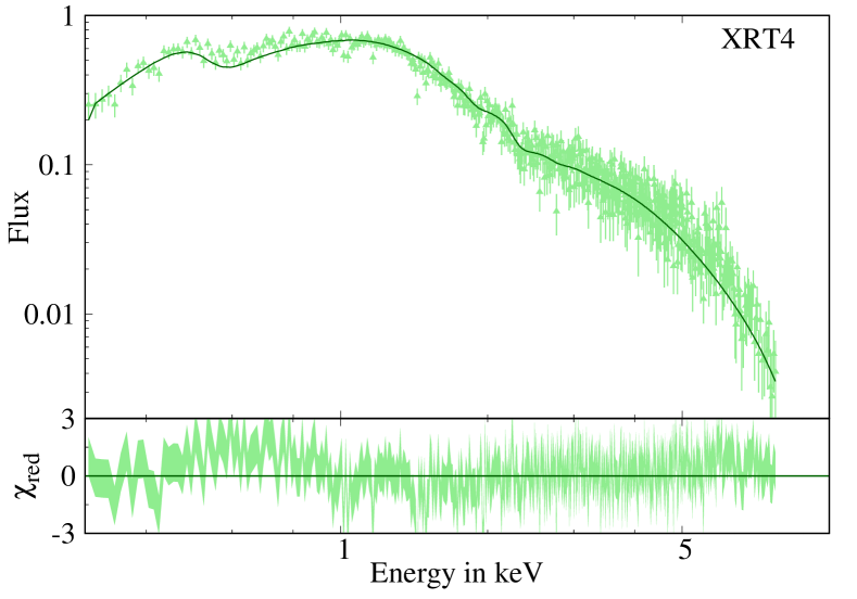
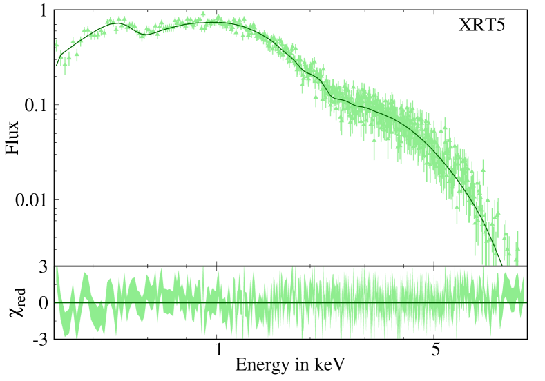
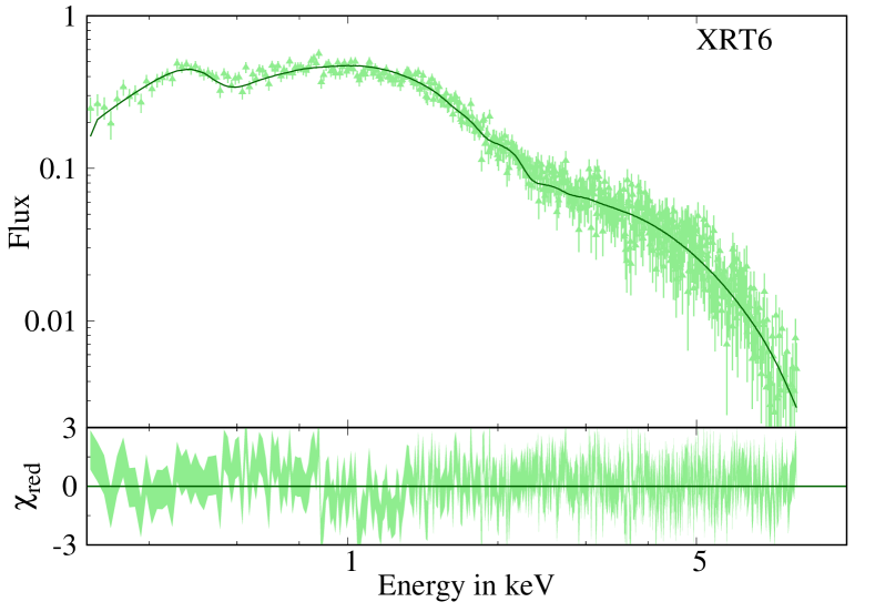
Figure 2: TCAF model fitted spectra of Ark 120 from the XMM-Newton, Suzaku, NuSTAR and Swift observations along with the residuals obtained from the spectral fitting.

Table 5: TBabs*zTBabs*(TCAF+zGaussian) model fitted Parameters in 0.2-79.0 keV energy band for Ark 120. The TBabs is fixed at $N_{H_{gal}}$= $9.78\times 10^{20}$ cm^-2. The second column shows the variation of zTBabs for z = 0.033.

ID	MJD	$N_{H}$	$M_{BH}$	$\dot{m}_{d}$	$\dot{m}_{h}$	$X_{s}$	$R$	$N_{TCAF}$	$\Gamma_{pexrav}$	$R_{ref}$	$N_{pexrav}$	$\chi^{2}/dof$
		$(10^{20}cm^{-2})$	$\rm(10^{8}M_{\odot})$	$(\dot{m}_{Edd})$	$(\dot{m}_{Edd})$	$(r_{g})$		$(10^{-3})$			($10^{-3}$)
XMM1	$\rm 52875$	$1.0^{+0.2}_{-0.2}$	$1.50^{+0.03}_{-0.03}$	$\rm 0.063^{+0.002}_{-0.002}$	$\rm 0.112^{+0.001}_{-0.001}$	$20.36^{+4.46}_{-4.55}$	$1.95^{+0.34}_{-0.33}$	$0.16^{+0.05}_{-0.05}$	$0.14^{+0.10}_{-0.08}$	$1.96^{+0.05}_{-0.09}$	$0.14^{+0.04}_{-0.05}$	$1026.20/842$
S1	$\rm 54191$	$1.4^{+0.1}_{-0.2}$	$1.49^{+0.04}_{-0.04}$	$\rm 0.126^{+0.002}_{-0.001}$	$\rm 0.191^{+0.001}_{-0.001}$	$21.44^{+4.96}_{-4.85}$	$1.66^{+0.54}_{-0.57}$	$233.6^{+54.26}_{-58.65}$	$1.46^{+0.15}_{-0.41}$	$0.642^{+0.71}_{-0.51}$	$5.09^{+1.05}_{-1.03}$	$1869.89/1673$
XRT1	$\rm 54675$	$1.6^{+0.6}_{-0.4}$	$1.49^{+0.19}_{-0.15}$	$\rm 0.064^{+0.005}_{-0.005}$	$\rm 0.110^{+0.004}_{-0.003}$	$30.08^{+5.36}_{-6.24}$	$2.80^{+0.54}_{-0.56}$	$0.54^{+0.01}_{-0.02}$	$-$	$-$	$-$	$307.78/283$
XMM2+N1	$\rm 54341$	$1.9^{+0.3}_{-0.2}$	$1.50^{+0.08}_{-0.07}$	$\rm 0.068^{+0.006}_{-0.005}$	$\rm 0.111^{+0.004}_{-0.004}$	$52.83^{+8.65}_{-8.56}$	$2.83^{+0.55}_{-0.52}$	$0.57^{+0.02}_{-0.02}$	$0.90^{+0.09}_{-0.10}$	$0.254^{+0.47}_{-0.06}$	$0.25^{+0.06}_{-0.05}$	$1230.15/1112$
XMM3+N2	$\rm 54738$	$2.3^{+0.3}_{-0.3}$	$1.51^{+0.09}_{-0.10}$	$\rm 0.103^{+0.006}_{-0.005}$	$\rm 0.126^{+0.004}_{-0.004}$	$28.24^{+5.04}_{-5.25}$	$2.43^{+0.55}_{-0.58}$	$0.31^{+0.01}_{-0.01}$	$1.66^{+0.19}_{-0.19}$	$0.96^{+0.05}_{-0.56}$	$0.12^{+0.06}_{-0.06}$	$1578.92/1359$
XRT2	$\rm 56926$	$2.5^{+0.1}_{-0.1}$	$1.49^{+0.18}_{-0.20}$	$\rm 0.068^{+0.005}_{-0.006}$	$\rm 0.110^{+0.003}_{-0.003}$	$53.56^{+8.27}_{-8.87}$	$2.73^{+0.51}_{-0.47}$	$0.36^{+0.01}_{-0.02}$	$-$	$-$	$-$	$579.89/555$
XRT3	$\rm 56974$	$1.9^{+0.5}_{-0.5}$	$1.51^{+0.19}_{-0.20}$	$\rm 0.068^{+0.006}_{-0.006}$	$\rm 0.110^{+0.004}_{-0.005}$	$55.16^{+8.57}_{-8.80}$	$2.74^{+0.45}_{-0.41}$	$0.25^{+0.01}_{-0.01}$	$-$	$-$	$-$	$630.08/594$
XRT4	$\rm 57024$	$1.1^{+0.2}_{-0.3}$	$1.50^{+0.15}_{-0.18}$	$\rm 0.061^{+0.006}_{-0.006}$	$\rm 0.110^{+0.005}_{-0.003}$	$56.86^{+10.97}_{-10.89}$	$2.69^{+0.48}_{-0.47}$	$0.11^{+0.01}_{-0.01}$	$-$	$-$	$-$	$702.39/548$
XRT5	$\rm 57073$	$1.4^{+0.4}_{-0.3}$	$1.49^{+0.16}_{-0.15}$	$\rm 0.069^{+0.006}_{-0.007}$	$\rm 0.110^{+0.005}_{-0.005}$	$57.87^{+12.99}_{-12.08}$	$2.77^{+0.52}_{-0.54}$	$0.28^{+0.02}_{-0.01}$	$-$	$-$	$-$	$551.49/531$
XRT6	$\rm 58118$	$2.0^{+0.4}_{-0.4}$	$1.51^{+0.16}_{-0.15}$	$\rm 0.081^{+0.006}_{-0.005}$	$\rm 0.140^{+0.006}_{-0.007}$	$42.95^{+8.98}_{-8.20}$	$2.69^{+0.59}_{-0.61}$	$0.22^{+0.01}_{-0.01}$	$-$	$-$	$-$	$612.9/589$

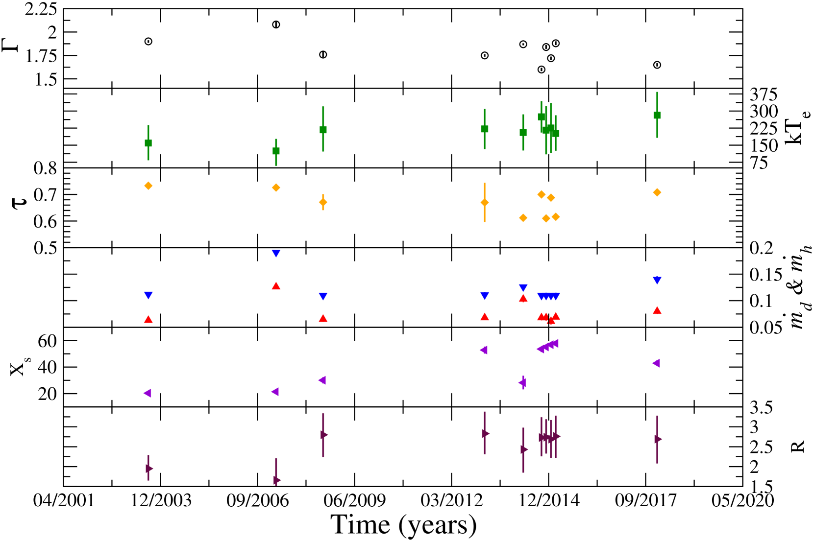
Figure 3: Variation of different model parameters with time are presented.

3.2 TCAF

From the nthcomp model fitting, we have extracted several valuable information on the spectral hardness and electron temperature of the emitting system in a time duration of $\sim$ 15 years. We have also calculated the optical depths from these parameters, which are shown in Table 2. However, the fundamental properties, such as the central black hole mass, accretion rates, the size of the Compton cloud radius could provide a deeper physical understanding of the system. To estimate these quantities, we use the Two-Component Advective Flow (TCAF) model (Chakrabarti & Titarchuk, 1995) for our spectral analysis. For the spectral fitting, the model in XSPEC reads as:

TBabs*zTBabs*(TCAF+zGaussian)

TCAF is based on one black hole parameter and four flow parameters: (i) black hole mass in units of the solar mass ($M_{\odot}$); (ii) Keplerian disc accretion rate ($\dot{m}_{d}$) in the unit of the Eddington rate ($\dot{M}_{EDD}$); (iii) Sub-Keplerian halo accretion rate ($\dot{m}_{h}$) in units of Eddington rate ($\dot{M}_{EDD}$); (iv) shock compression ratio (R) and (v) shock location ($X_{s}$) in units of the Schwarzschild radius ($r_{g}=2GM/c^{2}$). The upper and lower limits of all the parameters are put in a data file called lmodel.dat provided in Table-4 as an input to run the source code using initpackage and lmod task in XSPEC. For the final spectral fitting of a specified observation, we run the source code for a vast number of times and select the best spectrum from many spectra using minimization of $\chi$ method. First, we have started fitting by the baseline model described as above. Some spectra, like XMM1, S1, XMM2+N1, XMM3+N2 have high reduced $\chi^{2}$ ($\chi^{2}_{red}>2$) value. We noticed that the model has deviated from the actual data at the high energy end. To compensate for that, we have added a powerlaw/pexrav with the baseline model. Thus the model became:

TBabs*zTBabs*(TCAF+powerlaw/pexrav+zGaussian).

We have fitted the spectra with this model and found $\chi^{2}_{red}\approx 1$. Further, to investigate the source of this power-law (whether it is from reflection or not), we have replaced the powerlaw component by pexrav (Magdziarz & Zdziarski, 1995). The pexrav model has a power-law continuum with a reflected component from an infinite neutral slab. We have estimated the relative reflection coefficient ($R_{ref}$) with photon index ($\Gamma_{pexrav}$) and cosine of inclination angle $\cos\theta$ from the model fitting. We find $\theta$ to vary from $40\degree$ to $72\degree$. We fix abundances for heavy elements, such as iron at the Solar value (i.e., 1). For the photon index ($\Gamma_{pexrav}$), first, we freeze its value to the value of $\Gamma$ obtained from nthcomp. For this, we have found $\chi^{2}_{red}>2$. Thereafter, we thaw this parameter and fit it again which have resulted $\chi^{2}_{red}\approx 1$ with new value of $\Gamma_{pexrav}$.

We first fit the XMM-Newton observation (XMM1) during 2003 (MJD-52875) in the energy range of 0.2 to 10.0 keV with TBabs*zTBabs*(TCAF+zGaussian) model. However, we found a high $\chi^{2}_{red}$. The model has deviated after 9.2 keV from the actual data. As mentioned above, we then add a powerlaw with the baseline model, and then the powerlaw is replaced by pexrav. The fitted parameters are, $M_{BH}=1.5\times 10^{8}M_{\odot}$, $\dot{m}_{d}=0.063$, $\dot{m}_{h}=0.112$, $X_{s}=20.36$, $R=1.95$ with $\Gamma_{pexrav}=0.14$, $R_{ref}=1.96$, and $E_{fold}=16.08$ keV and the corresponding $\chi^{2}=1026.20$ with degrees of freedom (dof)= 842. The Fe line is found at $6.4$ keV with an equivalent width of $116$ eV.

Next, we consider the Suzaku observation (S1) of 2007 (MJD-54191). We combine the Suzaku/XIS and Suzaku/HXD spectra and make a broadband spectrum in the energy range of 0.5 to 40 keV. We follow the similar steps as described in XMM1 fitting and the fitted parameters are $M_{BH}=1.49\times 10^{8}M_{\odot}$, $\dot{m}_{d}=0.126$, $\dot{m}_{h}=0.191$, $X_{s}=21.44$, $R=1.66$ with $\Gamma_{pexrav}=1.46$, $R_{ref}=0.642$, and the corresponding $\chi^{2}_{red}/dof=1869.89/1673$. The position of Fe line is $6.38$ keV with an equivalent width of $710$ eV. It is to be noted that, within $6-7$ keV range, Nardini et al. (2011) reported the possibility of three lines for XMM1 and two lines for S1 observation respectively.

Following a similar procedure, we fit the broadband spectra of Ark 120 for the observations during 2013 XMM2+N1 (MJD-56341) and 2014 XMM3+N2 (MJD-56738). For these, we have obtained $M_{BH}=1.50$ & $1.51\times 10^{8}M_{\odot}$, $\dot{m}_{d}=0.068$ & $0.103$, $\dot{m}_{h}=0.111$ & $0.126$, $X_{s}=52.83$ & $28.24$, $R=2.83$ & $2.43$ with $\Gamma_{pexrav}=0.96$ & $1.66$ respectively. The details of data fitting are given in Table-5.

We fit all the six Swift/XRT spectra using the baseline model. Here, we do not find any Fe line in all these spectra. From the fitting, it is noticed that the mass of the central black hole $M_{BH}$ =$1.5\times 10^{8}M_{\odot}$, the disc $\dot{m}_{d}\sim 0.065$ and halo accretion rates $\dot{m}_{h}$$\sim 0.110$ are more or less constant except XRT6 observation. Here, we find $\dot{m}_{d}=0.081$ & $\dot{m}_{h}=0.14$ and the corresponding shock location has moved inward from 57.87 to 42.95 $r_{g}$. Therefore, the shock location ($X_{s}$) has varied in between $30.0$ to $57.87~{}r_{g}$, and the corresponding variation of the compression ratio (R) is in between $2.6$ to $2.8$ within September 2014 to January 2018. Here, we do not require any additional powerlaw to fit the high energy spectra. The details of the parameter variations are presented in Table-5. In Figure 2, we plot the model fitted spectrum with the variation of $\chi$. Detailed discussions on spectral properties are demonstrated in Sec 5.1.

Table 6: Variability statistics in various energy ranges are shown in this Table. We have opted for 100s time bins for variability analysis. In some cases, the average error of observational data exceeds the limit of $1\sigma$, resulting negative excess variance. In such cases, we have imaginary $F_{var}$, which are not shown in the table.

ID	Energy band	$N$	$x_{max}$	$x_{min}$	$\frac{x_{max}}{x_{min}}$	$\sigma^{2}_{NXS}$	$F_{var}$
	keV		Count/s	Count/s		$(10^{-2})$	$(10^{-2})$
XMM1	0.2-2.0	1117	21.95	19.58	1.12	$0.57\pm 0.003$	$1.6\pm 0.14$
XMM2	0.2-2.0	1294	10.24	8.40	1.21	$2.9\pm 0.015$	$5.6\pm 0.40$
XMM3	0.2-2.0	1309	21.37	17.11	1.25	$8.22\pm 0.011$	$6.4\pm 0.41$
XMM1	3-10.0	1117	1.95	1.53	1.79	$0.18\pm 0.023$	$3.2\pm 0.04$
XMM2	3-10.0	1294	1.22	0.94	1.30	$0.137\pm 0.035$	$3.5\pm 0.55$
XMM3	3-10.0	1309	3.64	2.92	1.24	$0.56\pm 0.0011$	$4.1\pm 0.34$
N1	10.0-78.0	722	0.711	0.105	6.748	$0.093\pm 0.007$	$7.5\pm 1.6$
N2	10.0-78.0	667	1.712	0.239	7.143	$0.147\pm 0.024$	$3.5\pm 3.6$
XMM1	0.5-10.0	1117	20.46	15.26	1.341	$10.11\pm 0.06$	$2.36\pm 0.14$
S1	0.5-10.0	586	9.80	5.58	1.76	$5.64\pm 0.31$	$8.62\pm 0.31$
XRT1	0.5-10.0	8	3.22	1.67	3.01	-$22.3\pm 5.6$	$-$
XMM2	0.5-10.0	1294	10.36	6.73	1.54	$2.93\pm 0.02$	$5.85\pm 0.19$
XMM3	0.5-10.0	1309	20.13	13.67	1.47	$5.80\pm 0.01$	$5.79\pm 0.15$
XRT2	0.5-10.0	50	2.13	0.70	3.02	$5.50\pm 0.44$	$20.70\pm 2.3$
XRT3	0.5-10.0	43	2.79	1.52	2.79	$3.61\pm 0.42$	$15.31\pm 2.1$
XRT4	0.5-10.0	43	1.90	0.88	2.16	$4.50\pm 0.46$	$18.01\pm 2.3$
XRT5	0.5-10.0	42	1.77	0.81	2.18	$2.72\pm 0.25$	$14.03\pm 1.8$
XRT6	0.5-10.0	72	1.63	0.52	3.09	$6.02\pm 0.49$	$23.40\pm 2.2$

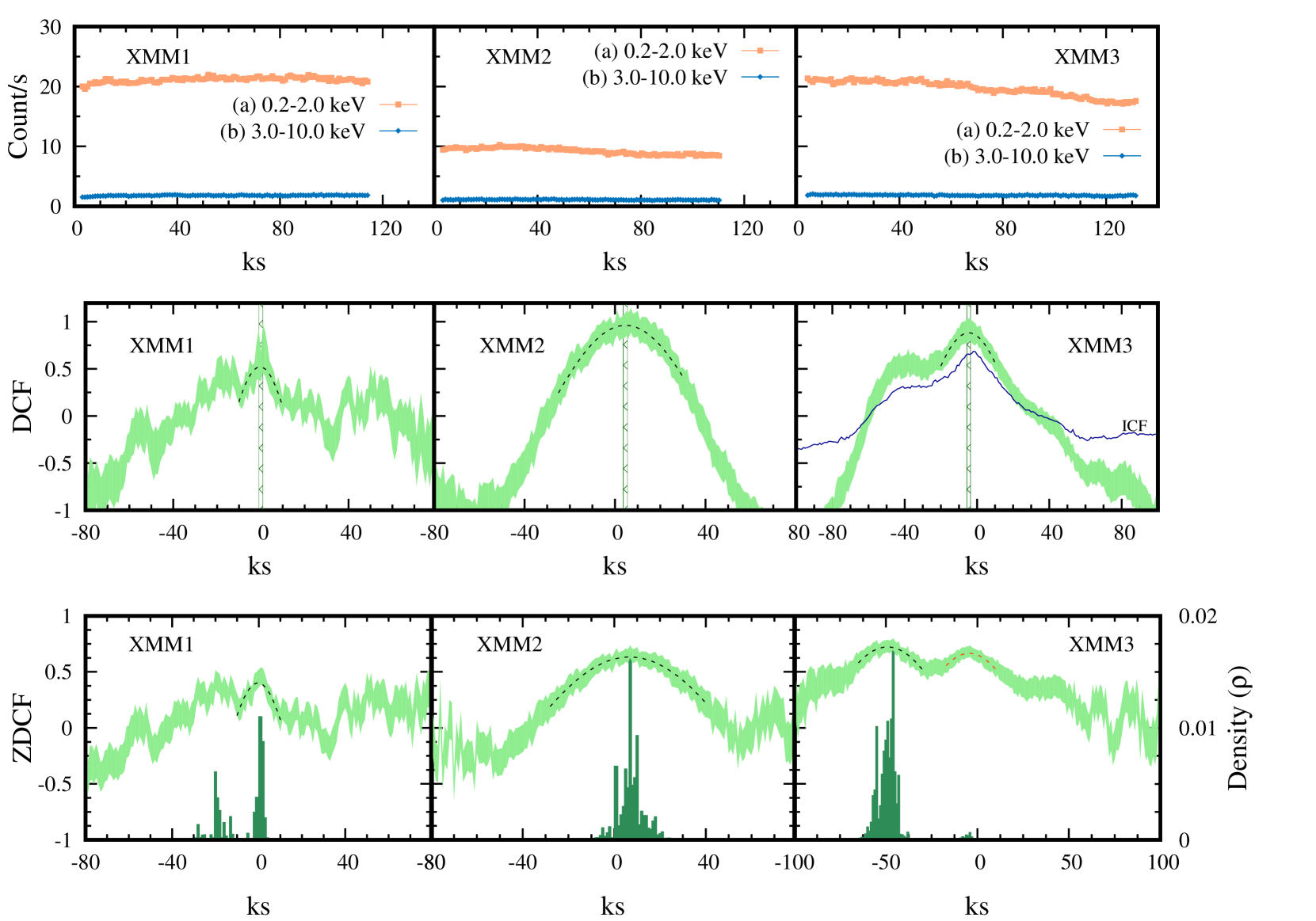
Figure 4: Top panel: The light-curves of the energy ranges of $0.2$ to $2.0$ keV and $3.0$ to $10.0$ keV observed by XMM-Newton are plotted for three epochs. The high energy count always remained a fraction of low energy counterpart. In 2013, the low-energy count dropped to nearly 50% as compared to 2003. Again in 2014, the $0.2-2$ keV count doubled from its value observed in 2013. Middle panel: Corresponding discrete cross-correlations between light-curves of $0.2-2$ keV and $3-10$ keV are plotted. All three epochs exhibited different patterns where zero, positive, and negative delays are observed in 2003, 2013, and 2014 respectively. We have also presented the ICF (solid-blue line) for XMM3 observation. Lower panel: $\zeta$-discrete cross-correlations (light-green) are plotted for light-curves of $0.2-2$ keV and $3-10$ keV. While 2003 and 2013 patterns remain similar to what have been observed from DCF, the pattern obtained from 2014 data develops twin peak. The likelihoods (dark-green), simulated using 12000 points, are plotted along with the ZDCF.

4 Timing Analysis

4.1 Variability

X-ray variability of an AGN provides a powerful probe of the nearby regions of the central black hole. Since Ark 120 has a ‘bare-type nucleus’, the X-ray comes from the Compton cloud and is not intercepted by any clouds such as BLR, NLR or molecular torus. Thus, the X-ray variability is originated from the varying Compton cloud and the central accretion disc. To analyze the temporal variability in X-ray of Ark 120 in different energy bands, we have estimated different parameters for the duration of 2003 (MJD-52875) to 2018 (MJD-58118). The fractional variability $F_{var}$ ((Edelson et al., 1996); (Nandra et al., 1997); (Edelson et al., 2001); (Edelson et al., 2012); (Vaughan et al., 2003); (Rodríguez-Pascual et al., 1997)) of lightcurves of $x_{i}$ count/s with finite measurement error $\sigma_{i}$ of length $N$ with a mean $\mu$ and standard deviation $\sigma$ is given by:

$$F_{var}=\sqrt{\frac{\sigma^{2}_{XS}}{\mu^{2}}}$$ (2)

where, $\sigma^{2}_{XS}$ is excess variance (Nandra et al. (1997); Edelson et al. (2002)), an estimator of the intrinsic source variance and is given by:

$$\sigma^{2}_{XS}=\sigma^{2}-\frac{1}{N}\sum_{i=1}^{N}\sigma^{2}_{i}.$$ (3)

The normalized excess variance is given by $\sigma^{2}_{NXS}=\sigma^{2}_{XS}/\mu^{2}$. The uncertainties in $\sigma^{2}_{NXS}$ and $F_{var}$ are taken from Vaughan et al. (2003) and Edelson et al. (2012).

The X-ray variability of Ark 120 in different energy bands ($0.5-10.0$ keV; $0.2-2.0$ keV; $3.0-10.0$ keV) have demonstrated different degrees of variabilities (Table 6) while the time binsize is kept constant at $100$s. From XMM1, the lower energy ($0.2-2.0$ keV) count rate was initially high ($X_{max}=21.95$) in 2003 observation. Then, in 2013 (XMM2), it became half ($X_{max}=10.24$) from its initial value. In 2014 (XMM3), the count increased ($X_{max}=21.37$). The fractional variability in this energy range increased from $0.016$ to $0.064$ from 2003 to 2014 observations. A similar trend is shown by $\sigma^{2}_{NXS}$ ($0.006$ to $0.082$) in this energy band for each observation of XMM (Table 6). Like low energy part, the high energy ($3.0-10.0$ keV) follow the similar type of trend for the count rate and fractional variability. The average value of $\sigma^{2}_{NXS}$ is $0.003$, with a range from $0.0014$ to $0.0056$.

We calculate the variability in $0.5-10.0$ keV range from the Suzaku data. We find higher variability $F_{var}=8.62\pm 0.31$ in the 2007 Suzaku data as compared to the previous XMM observations. The variability for XRT observations in $0.5-10.0$ keV range is shown in Table 6. Due to the lack of data points, XRT1 observation yields an imaginary value of $F_{var}$, and is not shown in Table 6. From the other observations of Swift/XRT, we observe high fractional variability ($F_{var}$) from $0.14$ to $0.23$ with $<F_{var}>=18.22$. The average value of $x_{max}/x_{min}$ and $\sigma^{2}_{NXS}$ for these observations are $2.65$ and $0.045$ with a range from $2.16$ to $3.09$ and $0.027$ to $0.060$ respectively.

4.2 Delay Estimation

For temporal analysis of the long term archival data of Ark 120, we stress three epochs of XMM-Newton, 2003, 2013, and 2014 out of which the latter two have high energy (3-80 keV) counterparts observed by NuSTAR. We have performed cross-correlation analysis using DCF (Edelson & Krolik, 1988) and $\zeta$-discrete cross-correlation function (ZDCF, Alexzander (1997)) for comparison. The likelihood is calculated using 12000 simulation points in the ZDCF code for the lightcurves obtained by XMM-Newton. The peak error is calculated using the formula provided by Gaskell & Peterson (1987). We have followed a similar procedure as in Chatterjee et al. (2020). The time resolution of each light curve is $1000$s. The $0.2-2$ keV lightcurve obtained from 2003 data yields an acceptable $\chi^{2}_{red}<1.5$ when fit with a straight line. However, data procured in 2013 and 2014 in a similar energy band have a high residual and are not suitable for linear fitting. All three high energy lightcurves (3-10 keV) have $\chi^{2}_{red}<1.5$ when fitted with straight lines. We have carried out the delay estimation using the XMM-Newton/Epic-pn data to ensure the simultaneity in their procurements.

Table 7: Parameters used in delay estimations are presented. The error in measurement of delay is considered as the larger between binsize and $\epsilon_{\tau}$. $\epsilon^{d}_{\tau}$ and $\epsilon^{z}_{\tau}$ represents errors for DCF and ZDCF patterns.

Id	Epochs	Bin size	$\epsilon^{d}_{\tau}$	$\Delta\tau^{dcf}_{d}$	$\epsilon^{z}_{\tau}$	$\Delta\tau^{zdcf}_{d}$
	Year	(ks)	(ks)	(ks)	(ks)	(ks)
blackXMM1	2003	1	0.388	$0.16\pm 1$	0.936	$-0.057\pm 1$
blackXMM2	2013	1	0.862	$4.71\pm 1$	2.11	$6.76\pm 2.11$
blackXMM3	2014	1	0.622	$-4.15\pm 1$	1.54	$-4.56\pm 1.54$
blackXMM3	2014	1	$-do-$	$-do-$	1.58	$-49.2\pm 1.58$

The DCF (Edelson & Krolik, 1988), performed using the lightcurves, have generated three distinct patterns. The 2003 data has produced $2.78\pm 16.67$ minutes or $\sim 0.16$ ks delay. We have fitted the peak using a Gaussian model (dotted line in Fig. 4). Considering the error, no delay can be seen between two bands of X-ray. Similar delay pattern is also observed from ZDCF, and the likelihood density also maximizes around zero. Likewise, we have performed Gaussian fitting for 2013 data where a positive delay of $78.51\pm 35.17$ minutes or $\sim 4.7$ ks has been seen between soft and hard X-ray photons using DCF. But, the ZDCF peak maximizes around $112.68\pm 35.22$ minutes or 6.7 ks and likelihood peak coincides with that (see Fig. 4). In 2014, the delay sign have switched, and we find a negative delay of $-69.19\pm 25.67$ minutes or $\sim-4.1$ ks between the soft and hard band from DCF analysis. However, ZDCF peaks maximize around two positions, $-76.19\pm 25.67$ ($-4.56\pm 1.54$ ks) and $-820.19\pm 26.46$ ($-49.2\pm 1.58$ ks) minutes having peak values of 0.664 and 0.722 respectively. Between these two, the former coincides with the DCF pattern (see, Table 7 for details). For all three cases, we find the peak values of ZDCF patterns are lesser than the corresponding peak values obtained from DCF patterns.

5 Discussions

We have studied the central region of Ark 120 through X-ray (above 0.2 keV) using the data of XMM, Suzaku, NuSTAR and Swift/XRT in the period 2003 (MJD-52875) to 2018 (MJD-58118). As it is a bare type AGN, the X-ray spectra mainly generated from the nearby region of the central engine.

5.1 Evolution of the Source: Primary Continuum

The ‘bare-type AGN’ Ark 120 was observed for a period of fifteen years, 2003 to 2018 using various X-ray satellites. During these observations, the source has exhibited variabilities in both spectral and temporal domain. The luminosity of the source in the energy range of 2.0 to 10.0 keV varied within $\sim 10^{43.5}-10^{45.5}$ erg/s throughout these observations. From the nthcomp model, we report the variation of the spectral index (1.6<$\Gamma$<2.08) where the harder spectra were observed after 2014. Following Vaughan et al. (2004), we have fitted the 2003 spectrum of Ark 120 with (nthcomp + Gaussian) model. The fitted $\Gamma=1.90^{+0.01}_{-0.01}$ agrees with the spectral index previously observed (Table 4 of Vaughan et al. (2004)). Corresponding temperature of the Compton cloud is $kT_{e}=159.45^{+81.68}_{-81.69}$ keV. The (TCAF + Gaussian) model provided a few previously unknown parameters like accretion rates, disc rate $\dot{m}_{d}=0.063\pm 0.002$ and halo rate $\dot{m}_{h}=0.112\pm 0.001$. This suggests that the the source was initially halo dominated. This is normal for an AGN. The shock location or the size of the CENBOL ($X_{s}$), estimated from the fits, is $20.36\pm 4.4~{}r_{g}$. The shock is found to be moderately strong with a compression ratio of $R=1.95\pm 0.05$.

The softest spectrum, having $\Gamma=2.08^{+0.03}_{-0.03}$ is seen during the Suzaku observation in 2007. It is to be noted that, Nardini et al. (2011) found the spectral index to be $\Gamma=2.03^{+0.01}_{-0.04}$ for the Suzaku data using blurred reflection model. We have estimated the temperature of the Compton cloud to be $kT_{e}=124.65^{+35.54}_{-35.21}$ keV. This is the least of all temperatures obtained from all the observations. Using a single Gaussian, we find the presence of a broad iron line ($6.38^{+0.052}_{-0.052}$) keV having an equivalent width of $EW=710^{+10}_{-10}$ eV. The derived optical depth is $\tau=0.726^{+0.008}_{-0.008}$. This suggests an optically thin Compton cloud. From the TCAF fits, we find that the size of the Compton cloud has slightly increased to $X_{s}=21.44\pm 4.9~{}r_{g}$ from the earlier observation. Corresponding disc rate, which enhances the soft seed photons, has increased to $\dot{m}_{d}=0.126$. Also, the halo rate has increased to $\dot{m}_{h}=0.191$. However, shock strength has decreased (see Table 5). The drop in the $kT_{e}$ could be understood easily from TCAF, where the increase in disc rate leads to an enhanced cooling fraction. Thus, within the epochs of 2003 and 2007, the temperature of the Compton cloud was varied from 159.45 to 124.65 and as a result the spectrum softened.

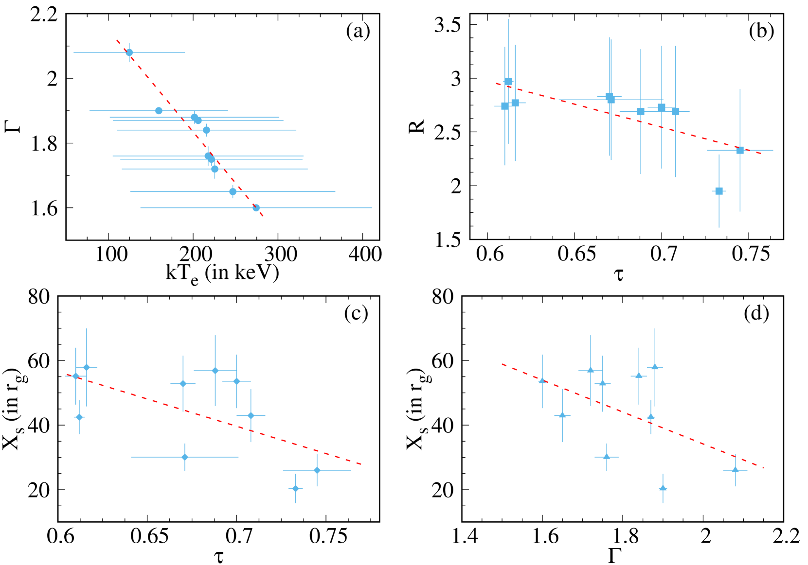
Figure 5: Correlation of fitted parameters are plotted. Fig. (a) represents the correlation between $\Gamma$ vs $kT_{e}$ and the corresponding PCC is -0.95. It is also noted that the $kT_{e}$ is losely bound with $\Gamma$. Fig. (b) is the correlation between $\tau$ and R. The PCC for these parameters is -0.72. In Fig. (c) represents the correlation between $\tau$ vs $X_{s}$ and the corresponding PCC is -0.45. Fig. (d) provides the correlation of $\Gamma$ vs $X_{s}$ with PCC -0.53.

Later, in 2008, Swift observed the source where the spectrum hardened from the previous observation having $\Gamma=1.76^{+0.02}_{-0.08}$, $kT_{e}=217.72^{+105.6}_{-112.5}$ keV, and optical depth $\tau=0.671^{+0.030}_{-0.030}$. The iron line could not be detected from the XRT spectrum. Corresponding TCAF fitted parameters, such as the shock location $30.08~{}r_{g}$ and $R=2.80$ while $\dot{m}_{d}$ and $\dot{m}_{h}$ have changed to $0.064$ and $0.11$ respectively.

Significant variation of spectral properties is also noted during 2013 and 2014. The broad-band spectra (3-78) keV are fitted with (nthcomp + Gaussian) having the spectral indices $1.75^{+0.01}_{-0.02}$ and $1.87^{+0.01}_{-0.01}$ and are in good agreement with parameters obtained by Porquet et al. (2018); Marinucci et al. (2019). The optical depth is reduced from $\tau=0.670\pm 0.074$ to $\tau=0.612\pm 0.003$. The flux in 2-10 keV band has doubled within a year. The spectral softening could be explained by the drop of temperature of the Compton cloud. However, the decrease in the optical depth for March 2014 data with respect to 2013 has also been seen from Monte-Carlo simulations (Marinucci et al., 2019). From TCAF fitting, we find a distinct variation of the flow parameters. The $\dot{m}_{d}$ changed from $0.068$ to $0.103$, $\dot{m}_{h}$ changed from $0.111$ to $0.126$, and $X_{s}$ changed from $52.83$ to $28.24$ within 2013 and 2014 observations respectively. As the disc accretion rate increases, Compton cooling increases, and this lead to the decrease in the $X_{s}$ which finally softens the spectrum. Considering TCAF, the lower optical depth for softer spectrum could be explained by the weakening of the shock ($R=2.43$ as compared to $R=2.83$ in February 2013) for this observation. The stronger shock creates a distinct boundary between the halo and CENBOL region where the majority of the hard photons are produced. However, for the weaker shock, the CENBOL boundary is less sharp and a fraction of inverse Comptonization could occur within the halo component. Thus, the effective optical depth of the medium could become lower even though the spectrum has softened.

Ark 120 has shown significant variabilities after February 2014 and is monitored by Swift. We have tabulated the spectral and temporal variabilities in Table 2 and 5. During September-October of 2014, we find that the spectral slope was $\Gamma=1.60^{+0.01}_{-0.02}$ and the corresponding temperature was $274.40\pm 130.0$ keV, which was maximum within the duration of our observation. From the TCAF fitting, we find $\dot{m}_{d}$ and $\dot{m}_{h}$ has changed to $0.068$ and $0.11$ respectively and the corresponding shock location has changed to $53.56\pm 8.2~{}r_{g}$ and the shock strength has increased from $2.43$ to $2.73\pm 0.5$ as observed during February 2014. Later, in December 2014, the spectrum has softened with $\Gamma=1.84\pm 0.02$ with the temperature of Compton cloud $215.72\pm 105.5$ keV. The corresponding shock has moved outward and observed at $55.16~{}r_{g}$ and $R=2.74$. Like previous observations, we see the halo rate and disc rates are fixed at $0.11$ and $0.068$, respectively.

XRT4 and XRT5 observations were made starting from the end of December 2014 to March of 2015. During this time, the spectral indices are $1.74$ and $1.88$ respectively. The temperature and optical depths have also varied during this time. From TCAF fitting, we find the halo rate has decreased to $0.061$ in the XRT4 observation. However, the disc rate was constant. Again in XRT5 observation, halo rate has increased to $0.069$ while the disc rate remained the same. The shock location and the compression ratio remained constant (considering the errors) within this period. Thus, we can see that Ark 120 exhibited spectral variability (see Fig. 3) within $\sim$200 days (since September 2014-March 2015).

In XRT6, which was observed from December 2017 to January 2018, the spectrum of Ark 120 has hardened with respect to the earlier observations during January 2015. The spectral index and temperature of Compton cloud are $1.65\pm 0.02$ and $246.87\pm 121$ keV respectively. From TCAF fitting, we find the disc and halo rates have increased to $\dot{m}_{d}=0.081$ & $\dot{m}_{d}=0.14$ respectively and the corresponding shock location settled at $42.95\pm 8.0~{}r_{g}$.

In Figure 5, we have plotted the correlations of a few spectral parameters. We find the spectral index and the temperature of the Compton cloud is anti-correlated (Fig. 5a with Pearson Correlation Co-efficient (PCC) = -0.9542) for the long term observation. However, the values of $kT_{e}$ are poorly constrained with respect to spectral indices. This is a well-established relation and is generally found in case of AGNs and Galactic black holes. In Fig. 5b, we have presented the correlation between shock compression ratio and optical depth. We find $R-\tau$ produces anti-correlation having PCC=-0.721. In general, stronger shocks are associated with the harder spectra where the optical depth is expected to be less (Chatterjee et al., 2016) and the corresponding shock location is also expected to be bigger. Keeping that argument, we also show the $X_{s}-\tau$ correlation where an anti-correlation (PCC=-0.457) has been observed from the long term data and presented in Fig. 5c. As a consequence, the spectral softens due to the reduction of the shock location $X_{s}$ i.e., the size of the Compton cloud, we find a global trend of anti-correlation (PCC=-0.562) between $X_{s}-\Gamma$ (see Fig. 5) for Ark 120.

From the nthcomp fitting, it can be found that the Compton cloud of the source was optically thin for the entire period of observation. Overall, we also noticed that the disc and halo rate is nearly constant and they are $\sim 0.07$ and $\sim 0.11$ respectively for the majority of observations. But, we find a higher disc and halo rate in 2007 and 2014 observation. The shock location and the compression ratio have varied with time. The variation of these parameters is shown in Figure 3. First, the shock location increases with time from 20 to 52 $r_{g}$ in the first $\sim 10$ years. Then the shock location falls to 26.7$r_{g}$ within the next $\sim$ 13 months. Later, we find that the shock location again moves outward from 26.7 to 57.8 $r_{g}$ before moving inward again, and finally settling at 42.95$r_{g}$ in January 2018. The Compression ratio (R) also varies as the shock location ($X_{s}$). First, the compression ratio increased from 1.95 to 2.83 in $\sim 10$ years. Then, the value of $R$ decreased to $1.67$ within next 1 year. After that, it increased to 2.73 within less than six months and finally reached 2.69 at the end of January 2018.

5.2 Evolution of the Source: Delay patterns

The Compton delay (Payne, 1980; Sunyaev & Titarchuk, 1980) for an electron cloud of size $\mathcal{R}$ having an optical depth $\tau$ and temperature $\theta_{e}=kT_{e}/m_{e}c^{2}$ can be described by,

$$t_{c}=\frac{\mathcal{R}}{c(1+\tau)}\frac{ln(E_{h}/E_{ss})}{ln[1+4\theta_{e}(1+4\theta_{e})]},$$

where, $c$ is the velocity of light, $E_{h}$ and $E_{ss}$ are the energy of hard photons and soft seed photons respectively. For AGNs having a central black hole mass of $1.5\times 10^{8}$ (Peterson et al., 2004), the seed temperature of the photons remains in the 1-10 eV range. The maximum of the hard and soft energy band is considered to be $10$ keV and $1$ keV and the seed photon temperature is $E_{ss}=3$ eV. The light-crossing time for 1$r_{g}$ is $r_{g}/c=$1.5 ks for Ark 120. We calculated the delays for the combined parameters obtained from nthcomp and TCAF model.

We have calculated the Compton delay for XMM1 observation where the size of the Compton cloud is $\sim 20~{}r_{g}$, optical depth $0.733$, and $\theta_{e}=0.311$. Substituting the values, we find $t^{h}_{c}=105.3$ ks and $t^{s}_{c}=75.3$ ks which produces a positive theoretical delay of $\Delta\tau=t^{h}_{c}-t^{s}_{c}=30$ ks. However, from the observed DCF pattern, we fail to notice any such delay for this case. Here, we find light crossing delay ($\tau_{lc}$) of 30 ks for a $\sim 20~{}r_{g}$ Compton cloud. The observed zero-delay could be a combined result of $\tau_{c}$ and $\tau_{lc}$. In that case, it is to be noted that $\tau_{lc}$ becomes crucial in presence of a significant contribution of reflection component ($R_{ref}=1.96$, see Table 5).

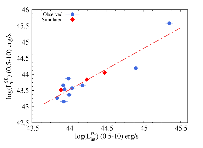
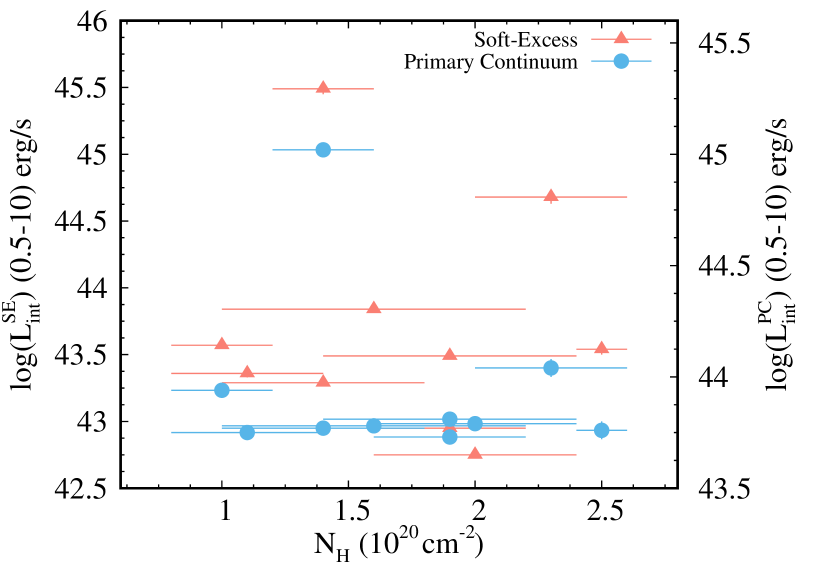
Figure 6: Correlation of intrinsic luminosities of 0.5-10.0 keV obtained using nthcomp. Left: shows a correlation (PCC=0.92) between the observed intrinsic luminosities of primary continuum and soft-excess (blue-circle). Monte-Carlo simulated luminosities for both energy ranges are presented with red-diamond points. Right: No correlation between intrinsic luminosities and $N_{H}$ from long term observations.

For the broadband observation (XMM2+N1), the size of the Compton cloud is $\mathcal{R}\sim 50$ $r_{g}$, having an optical depth of $0.67$ and temperature $\theta_{e}=0.434$. Combining all these, the maximum hard and soft energy delay which can be generated via Compton scatterings are $t^{h}_{c}=208$ ks and $t^{s}_{c}=148$ ks respectively. Thus, the maximum delay between hard and soft bands of X-ray can be $\Delta\tau=t^{h}_{c}-t^{s}_{c}=60$ ks. The light crossing delay is around $\tau_{lc}=75$ ks. The combined effects of $\Delta\tau$ and $\tau_{lc}$ should yield a negative delay of 15 ks. However, as discussed previously, $\tau_{lc}$ could dominate if reflection becomes dominating (here $R_{ref}=0.25$). Also, the size of the Compton cloud is much bigger than the what should be the ‘transition radius’ (see, Dutta & Chakrabarti (2016); Dutta, Pal & Chakrabarti (2018) for details) of an AGN having mass $1.5\times 10^{8}~{}M_{\odot}$. Being an intermediate inclination angle source (Nardini et al., 2011; Marinucci et al., 2019), Comptonization dominates the time delay when the size of the Compton cloud is bigger. The theoretical structure of Compton cloud is somewhat deviated from the sphere (see, Chakrabarti & Titarchuk (1995)) and the thermodynamical fluctuations within the inhomogeneous Compton cloud (see, Chatterjee et al. (2017b)) contributes to the delay patterns. Considering this, the effect of light crossing delay would be much less and Comptonization could be considered as the core process, which generates $0.2-2$ keV photons during 2013 observations.

In a similar way, we calculate the Compton delay for broadband observation in 2014 (XMM3+N2). For that, the size of the Compton cloud $\mathcal{R}=28~{}r_{g}$, the optical depth is $\tau=0.612$, and $\theta_{e}=0.403$. We have obtained $t^{h}_{c}=123.4$ ks and $t^{s}_{c}=88.2$ ks which produces $\Delta\tau=t^{h}_{c}-t^{s}_{c}=35$ ks. Contrary to that, the observed delay is $-69.19\pm 16.67$. Clearly, the Comptonization may not be the dominating radiative process for this observation. From Table 5, we see that the reflection co-efficient $R_{ref}=0.96$, which refers to a stronger reflection. It is also to be noted that Lobban et al. (2018) found the X-ray to be leading the U-band by $2.4\pm 1.8$ days which they have explained with the light crossing delay. Considering the Compton cloud only, $\tau_{lc}$ becomes 42 ks, which is comparable to compensate for the positive lag obtained from Comptonization. In this particular case, the maximum possible negative delay would be $\Delta\tau-\tau_{lc}\sim-7$ ks or -116 minutes. However, as the size of the Compton cloud has become bigger and $R_{ref}$ is much less than the XMM1 observation. Thus, the contribution from $\tau_{lc}$ could be less effective and we observe a negative delay much less than the maximum allowed delay.

Thus, along with the spectral variations, we find the delay patterns have varied over the three epochs (2003, 2013, and 2014) in which XMM-Newton observed Ark 120. A significant change in the delay pattern is observed within a year (2013-2014) where the positive delay changed sign and becomes negative with a similar magnitude.

5.3 Soft Excess

The origin of ubiquitous soft-excess (Arnaud et al., 1985; Singh et al., 1985; Brandt et al., 1993; Fabian et al., 2002; Gierliński & Done, 2004) remains debated. A plausible cause of soft-excess was given using reflection Sobolewska & Done (2007). The multi-wavelength campaign of Mrk 509 (Mehdipour et al., 2011) revealed the correlation of soft-excess with the optical-UV part both in the spectral and temporal domains where they concluded that the soft-excess was generated due to Comptonization by a warm optically thick region surrounding the accretion disc. Done et al. (2012) proposed that the high mass accretion rate of the disc could generate the soft-excess. For lower $L/L_{EDD}$, the energy dependent variability in the soft-excess part was found to be less in case of Narrow line Seyfert 1 galaxies. Lohfink et al. (2012) studied Seyfert 1 galaxy Fairfall 9 where the origin of the soft-excess component was found to be connected with source which generates the broad iron line. However, they implied that another source of Comptonization might be responsible for the formation of the soft-excess.

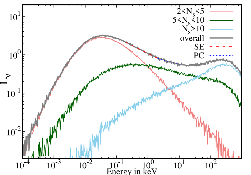
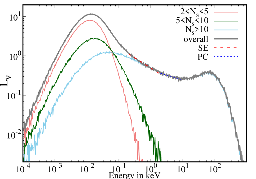
Figure 7: Monte-Carlo simulated spectra for Ark 120 are presented. We have considered $M_{BH}=1.5\times 10^{8}~{}M_{\odot}$ for Ark 120. Simulation boundary extends up to $100~{}r_{g}$. For left panel $\dot{m}_{d}$ = 0.06; $\dot{m}_{h}$ = 0.1, $X_{s}=60~{}r_{g}$, and maximum $kT_{e}=270$ keV. For right panel $\dot{m}_{d}$ = 0.1; $\dot{m}_{h}$ = 0.1, $X_{s}=40~{}r_{g}$, and maximum $kT_{e}=100$ keV. Notice the spectral contributions due to increasing number of scatterings. $L_{\nu}$ has been normalized with respect to the observed spectrum.

A strong soft-excess present in the X-ray spectrum of Ark 120 was reported by Brandt et al. (1993); Matt et al. (2014); Porquet et al. (2004). This soft-excess is also free from the absorbers and was reported by Nardini et al. (2011). As a first step, we investigate the spectral slopes and the relative contribution of the soft-excess from 2003 to 2018 using the nthcomp+zGaussian+powerlaw model and the results are presented in Table 3. Subsequently, we freeze the $\Gamma^{nth}$ obtained from nthcomp while fitting the soft excess below 3 keV. The $\Gamma^{pl}$ fits the soft-excess < 3 keV. For every observation, we find a soft-excess steeper than the primary continuum (see, Table 3) which is a characteristic associated with the Narrow line Seyfert 1 galaxies. Apart from the steeper power law, the variation of soft-excess luminosity and spectral index can be observed from long term observations presented in Table 3. We have calculated the intrinsic luminosities of nthcomp and powerlaw within the energy range 0.5 to 10.0 keV. In Fig. 6a, we see a strong correlation (PCC=0.9227) between the intrinsic luminosities of soft-excess ($L^{SE}_{int}$) and primary continuum ($L^{PC}_{int}$). However, as a “bare” type AGN, Ark 120 has not shown any correlation (Fig. 6b) among the intrinsic luminosities and the line of sight hydrogen column density ($N_{H}$).

While nthcomp provides a good fit in the high energy range, we have used TCAF+zGaussian+pexrav model (presented in Table 5) in the entire range. We find that the TCAF fits well in the range of $0.2-10$ and requires no other additional model for the soft-excess part with the range of $0.2-3$ keV. The fitted results and residuals are presented in Fig. 2. From the spectral fitting using TCAF, one recognizes that the soft-excess could be originated from the photons which are rarely scattered in the Compton cloud. The surrounding halo will contribute to this energy band (0.2 - 2 keV). Also, some high energy photons from the Compton cloud which could be reflected from the disc will appear in this energy range after losing their energy through reflection from the cold disc. We have performed Monte-Carlo simulations to show the spectral variations with $N_{s}$. This is briefly discussed in Sec. 5.3.1.

5.3.1 Simulated spectra

Radiative and hydrodynamic origin of soft-excess has been investigated in Fukumura et al. (2016) where they proposed that the shock heating near the ISCO could produce the soft-excess. The model reproduced the spectra of “bare” Seyfert 1 galaxy, Ark 120. We have inspected the possibility of scattering dependent spectral contribution from the pre-shock and the post-shock regions (Chakrabarti & Titarchuk, 1995). We extend the work of Ghosh et al. (2011); Chatterjee et al. (2018) in case of AGNs considering Ark 120. Using the Total Variation Diminishing (TVD) scheme (Ryu et al., 1997), we inject matter having a halo rate of $0.1$ from the outer boundary at $200~{}r_{g}$. TCAF fitted parameters are used for the simulation setup and are mentioned in the Fig. 7. Considering the Keplerian disc in the equatorial plane ($z=0$), we construct the profile of the accretion disc following Shakura & Sunyaev (1973). The Monte-Carlo simulation ($0<r<100~{}r_{g}$) has followed the process provided by Pozdnyakov et al. (1983) and later extended by Ghosh et al. (2009); Chatterjee et al. (2017a). The simulations are performed using $10^{7}$ injected photons for each case. The emergent Comptonized spectra are plotted in Fig. 7. We show the variation of spectral components with respect to the number of scatterings (see also Ghosh et al. (2011)) within the region. From Fig. 7, we find that the spectra harden as the number of scatterings increase. The spectra of the primary component within the energy range 2.0 to 10.0 keV is dominated by the photons where the number of scatterings are $\geq 10$. However, the soft-excess, the red long-dashed line within 0.2-2 keV, is dominated by the contribution from photons which have suffered $\leq 10$ scatterings. A steeper spectral slope ($\Gamma^{SE}$) for soft-excess is achieved with respect to the primary component ($\Gamma^{PC}$) for both of the spectrum. This is similar to what has been observed for Ark 120 (Table 3). It is to be noted that, Boissay et al. (2016) studied the AGN 102 Sy1 and found that there is no link between the reflection and the soft excess. Instead, they indicated that the soft-excess could be related to the thermodynamical properties of Compton cloud and associated medium.

6 Conclusions

We have studied $\sim 15$ years of X-ray data of Ark 120. We find the source varied considerably within that time span. This source was previously reported to be a ‘bare-type AGN’ and we also find a similar nature of this source from the long term analysis. The X-ray count rate has increased by a factor of two in a few years, and it is not found to be related to the Hydrogen column density ($N_{H}$) since it is a ‘bare-type AGN’. Following are the major findings from our work.

1. The spectral slopes of the primary continuum ($\Gamma^{PC}$) and the soft-excess ($\Gamma^{SE}$) are not constant throughout our observational time span. $\Gamma^{PC}$ has varied between 1.60 and 2.08 whereas $\Gamma^{SE}$ between 2.52 and 4.23 from 2003 to 2018.

2. The variation is reflected in fitted parameters of TCAF, namely, the accretion rates and properties of the Compton cloud. From the spectral fitting using TCAF, we find that the disc rate ($\dot{m}_{d}$) and the halo rate ($\dot{m}_{h}$) have varied between $0.061$ and $0.126$ and between $0.108$ and $0.191$ respectively. The shock location ($X_{s}$) or the size of the Compton cloud and compression ratio ($R$) vary correspondingly. $X_{s}$ varies between $20.36$ and $57.87$, whereas $R$ varies between $1.66$ and $2.73$.

3. We focussed on the simultaneous observations in low ($0.2-2.0$ keV) and high ($3.0-10.0$ keV) energy X-ray band from XMM-Newton to calculate the time delay between them. We find that in XMM1 observation, there is no delay between the low and high energy band, while a positive delay of $4.71\pm 1$ ks is detected in XMM2 observation and a negative delay of $4.15\pm 1$ ks is seen in XMM3 observation. A correlated variability among the optical, UV, and X-ray bands have already been reported Lobban et al. (2020). Also, (Dutta & Chakrabarti, 2016; Chatterjee et al., 2017b) reported in a different context that the X-ray lag has a strong dependency on the geometric structure of the Comptonization region and orientation of the Keplerian disc. The net delay is a resultant effect of different physical mechanisms, e.g., Comptonization, reflection, focusing, and jet/outflow emission (Chatterjee et al., 2019; Patra et al., 2019). For the lower inclination and radio-quiet nature of Ark 120, the positive delay could be attributed to the Compton delay while reflection and light-crossing delay could contribute to the negative delay.

4. From the analysis of the long term data, we report that the luminosity is independent of Hydrogen column density ($N_{H}$). This is expected as the source has a negligible line-of-sight hydrogen column density ($N_{H}<5\times 10^{20}$). The luminosity of the primary continuum is highly correlated (PCC$\sim 0.92$) with the soft excess emission. From TCAF fitting and Monte-Carlo simulations using TCAF flow configurations, we show that the soft-excess spectral slope ($\Gamma^{SE}$) is the result of a fewer Compton scatterings in the Compton cloud and the primary continuum ($\Gamma^{PC}$) is the result of the higher number of Compton scatterings. Corresponding intrinsic luminosities obtained from simulations corroborate with the observed pattern.

Data Availability

We have used archival data for our analysis in this manuscript. All the softwares used in this manuscript are publicly available. Appropriate links are given in the manuscript.

References

- Alexzander (1997) Alexander T. 1997, ASSL, 218, 163
- Alloin et al. (1988) Alloin, D., Boisson, C., & Pelat, D. 1988, A&A, 200, 17
- Arnaud et al. (1985) Arnaud, K. A., Branduardi-Raymont, G., Culhane, J. L., et al. 1985, MNRAS, 217, 105
- Arnaud (1996) Arnaud, K. A. 1996, Astronomical Data Analysis Software and Systems V, 17
- Bennett et al. (2003) Bennett C. L. et al., 2003, ApJS, 148, 1
- Bianchi et al. (2009) Bianchi, S., Guainazzi, M., Matt, G., Fonseca Bonilla, N., & Ponti, G. 2009, A&A, 495, 421
- Boissay et al. (2016) Boissay, R., Ricci, C., & Paltani S. 2016,A&A, 588, A70
- Brandt et al. (1993) Brandt W. N., Fabian A. C., Nandra K., Tsuruta S., 1993, MNRAS, 265, 996
- Burrows et al. (2005) Burrows D. N. et al., 2005, Space Sci. Rev., 120, 165
- Chakrabarti (1989) Chakrabarti, S. K. 1989, MNRAS, 240, 7
- Chakrabarti (1990) Chakrabarti, S. K. 1990, MNRAS, 243, 610
- Chakrabarti (1990) Chakrabarti, S. K. 1990, Theory of Transonic Astrophysical Flows (Singapore: World Scientific) (C90)
- Chakrabarti & Titarchuk (1995) Chakrabarti, S. K., & Titachuk, L. G. 1995, ApJ, 455, 623
- Chakrabarti (1995) Chakrabarti, S. K. 1995, in 17th Texas Symp. Relativistic Astrophysics and Cosmology, Accretion Disks in Active Galaxies: The Sub-Keplerian Paradigm, Vol. 759, ed. H. Bohringer, G. E. Morfil, & J. Trumper (New York: New York Academy of Sciences), 546
- Chatterjee et al. (2016) Chatterjee, Debnath, Chakrabarti, et al., 2016, ApJ, 827, 88
- Chatterjee et al. (2017a) Chatterjee A., Chakrabarti S. K., Ghosh H., 2017a, MNRAS, 465, 3902
- Chatterjee et al. (2017b) Chatterjee, A., Chakrabarti, S. K., & Ghosh, H. 2017b, MNRAS, 472, 1842
- Chatterjee et al. (2018) Chatterjee, A., Chakrabarti, S. K., Ghosh, H., & Garain, S. 2018, MNRAS, 478, 3356
- Chatterjee et al. (2019) Chatterjee A., Dutta B. G., Patra P., Chakrabarti S. K. & Nandi P., 2019, Proceedings, 17, 8, doi:10.3390/proceedings2019017008
- Chatterjee et al. (2020) Chatterjee, A., Dutta B. G., Nandi P. & Chakrabarti, S. K., 2020, MNRAS, 497, 4222
- Condon et al. (1998) Condon, J. J., Yin, Q. F., Thuan, T. X., & Boller, T. 1998, AJ, 116, 2682
- Crenshaw et al. (1999) Crenshaw, D. M., Kraemer, S. B., Boggess, A., et al. 1999, ApJ, 516, 750
- Crummy et al. (2006) Crummy J., Fabian A. C., Gallo L., Ross R. R., 2006, MNRAS, 365, 1067
- Debnath et al. (2014) Debnath, D., Chakrabarti, S. K., & Mondal, S. 2014, MNRAS, 440, L121
- Denissyuk et al. (2015) Denissyuk, E. K., Valiullin, R. R., & Gaisina, V. N., 2015, Astron. Rep., 59, 123
- Dewangan et al. (2007) Dewangan G. C., Griffiths R. E., Dasgupta S., Rao A. R., 2007, ApJ, 671, 1284
- Done et al. (2012) Done C., Davis S. W., Jin C., Blaes O., Ward M., 2012, MNRAS, 420, 1848
- Doroshenko et al. (2008) Doroshenko, V. T., Sergeev, S. G., & Pronik, V. I. 2008, Astron. Rep., 52, 442
- Dutta & Chakrabarti (2016) Dutta, B. G., & Chakrabarti, S. K. 2016, ApJ, 828, 101
- Dutta, Pal & Chakrabarti (2018) Dutta B. G., Pal P. S. & Chakrabarti S. K., 2018, MNRAS, 479, 2183
- Edelson & Krolik (1988) Edelson R. A. & Krolik J. H., 1988, ApJ, 333, 646
- Edelson et al. (1996) Edelson R. A., et al., 1996, ApJ, 470, 364
- Edelson et al. (2001) Edelson R., Griffiths G., Markowitz A., Sembay S., TurnerM. J. L., Warwick R., 2001, ApJ, 554, 274
- Edelson et al. (2002) Edelson R., Turner T. J., Pounds K., Vaughan S., Markowitz A.,Marshall H., Dobbie P., Warwick R., 2002, ApJ, 568, 610
- Edelson et al. (2012) Edelson R., Malkan M., 2012, ApJ, 751, 52
- Evans et al. (2009) Evans P. A., Beardmore A. P., Page K. L., 2009, MNRAS, 397, 1177
- Fabian et al. (2002) Fabian A. C., Ballantyne D. R., Merloni A., Vaughan S., Iwasawa K., Boller Th., 2002, MNRAS, 331, L35
- Fender et al. (1999) Fender R. et al., 1999, ApJ, 519, L165
- Fender et al. (2004) Fender R. P., Belloni T. M., Gallo E., 2004, MNRAS, 355, 1105
- Fukumura et al. (2016) Fukumura, K., Hendry, D., Clark, P., et al. 2016, ApJ, 827, 31
- García et al. (2014) García J. et al., 2014, ApJ, 782, 76
- Gaskell & Peterson (1987) Gaskell C. M. & Peterson B. M., 1987, ApJS, 65, 1
- Ghosh et al. (2009) Ghosh H., Chakrabarti S. K., Laurent P., 2009, IJMPD, 18, 1693
- Ghosh et al. (2011) Ghosh H., Garain S. K., Giri K., Chakrabarti S. K., 2011, MNRAS, 416, 959
- Gierliński & Done (2004) Gierliński, M., & Done, C. 2004, MNRAS, 349, L7
- Gliozzi et al. (2017) Gliozzi, M., Papadakis, I. E., Grupe, D., Brinkmann, W. P., & Räth, C. 2017, MNRAS, 464, 3955
- Haardt & Maraschi (1991) Haardt F., Maraschi L., 1991, ApJ, 380, 51
- Haardt & Maraschi (1993) Haardt F., Maraschi L., 1993, ApJ, 413, 507
- Halpern (1984) Halpern, J. P. 1984, ApJ, 281, 90
- Harrison et al. (2013) Harrison, F. A., Craig, W. W., Christensen, F. E., et al. 2013, ApJ, 770, 103
- Ho (2002) Ho, L. C. 2002, ApJ, 564, 120
- Ichimaru (1977) Ichimaru, S., 1977, ApJ, 214, 840
- Jansen et al. (2001) Jansen, F., Lumb, D., Altieri, B., et al. 2001, A&A, 365, L1
- Kalberla et al. (2005) Kalberla P. M. W., Burton W. B., Hartmann D., Arnal E. M., Bajaja E., Morras R., Piöppel W. G. L., 2005, A&A, 440, 775
- Kollatschny et al. (1981) Kollatschny, W., Fricke, K. J., Schleicher, H., & Yorke, H. W. 1981a, A&A, 102, L23
- Kollatschny et al. (1981) Kollatschny, W., Schleicher, H., Fricke, K. J., & Yorke, H. W. 1981b, A&A, 104, 198
- Koyama et al. (2007) Koyama K. et al., 2007, PASJ, 59, 23
- Kuehn et al. (2008) Kuehn, C. A., Baldwin, J. A., Peterson, B. M., & Korista, K. T. 2008, ApJ, 673, 69
- Lobban et al. (2018) Lobban, A. P., Porquet, D., Reeves, J. N., et al. 2018, MNRAS, 474, 3237
- Lobban et al. (2020) Lobban A. P., Zola S., Pajdosz-Śmierciak U., Braito V., et al. 2020, MNRAS, 494, 1165
- Lohfink et al. (2012) Lohfink A. M., Reynolds C. S., Miller J. M., Brenneman L. W., Mushotzky R. F., Nowak M. A., Fabian A. C., 2012, ApJ, 758, 67
- Magdziarz & Zdziarski (1995) Magdziarz P., Zdziarski A. A., 1995, MNRAS, 273, 837
- Magdziarz et al. (1998) Magdziarz P., Blaes O. M., Zdziarski A. A., Johnson W. N., Smith D. A., 1998, MNRAS, 301, 179
- Mandal & Chakrabarti (2008) Mandal, S., & Chakrabarti, S. K. 2008, ApJ, 689, L17
- Marinucci et al. (2019) Marinucci, A., Porquet, D., Tamborra, F., et al. 2019, A&A, 623, A12
- Markoff et al. (2005) Markoff S., Nowak M. A., Wilms J., 2005, ApJ, 635, 1203
- Marziani et al. (1992) Marziani, P., Calvani, M., & Sulentic, J. W. 1992, ApJ, 393, 658
- Matt et al. (2014) Matt G. et al., 2014, MNRAS, 439, 3016
- Mehdipour et al. (2011) Mehdipour, M., Branduardi-Raymont, G., Kaastra, J. S., et al. 2011, A&A, 534, A39
- Nandi et al. (2019) Nandi, P., Chakrabarti, S. K., & Mondal, S., 2019, ApJ, 877, 65
- Nandra et al. (1997) Nandra K., George I. M., Mushotzky R. F., Turner T. J., YaqoobT., 1997, ApJ, 476, 70
- Nardini et al. (2011) Nardini, E., Fabian, A. C., Reis, R. C., & Walton, D. J. 2011, MNRAS, 410, 1251
- Nardini et al. (2016) Nardini, E., Porquet, D., Reeves, J. N., et al. 2016, ApJ, 832, 45
- Patra et al. (2019) Patra D., Chatterjee A., Dutta B. G., Chakrabarti S. K., Nandi P., 2019, ApJ, 886, 137
- Payne (1980) Payne D. G., 1980, ApJ, 237, 951
- Peterson et al. (1998) Peterson, B. M., Wanders, I., Bertram, R., et al. 1998, ApJ, 501, 82
- Peterson et al. (2004) Peterson B. M. et al., 2004, ApJ, 613, 682
- Popović et al. (2001) Popović, L. C̃, Stanić, N., Kubiŏela, A., & Bon, E. 2001, A&A, 367, 780
- Porquet et al. (2004) Porquet, D., Reeves, J. N., O’Brien, P., & Brinkmann, W. 2004, A&A, 422, 85
- Porquet et al. (2018) Porquet, D., Reeves, J. N., Matt, G., et al. 2018, A&A, 609, A42
- Porquet et al. (2019) Porquet, D., Done, C., Reeves, J. N., et al. 2019, A&A, 623, A11
- Poutanen & Svensson (1996) Poutanen J., Svensson R., 1996, ApJ, 470, 249
- Pozdnyakov et al. (1983) Pozdnyakov A., Sobol I. M., Sunyaev R. A., 1983, Astrophys. Space Sci. Rev., 2, 189
- Pringle et al. (1973) Pringle J. E., Rees M. J., Pacholczyk A. G., 1973, A&A, 29, 179-184
- Reeves et al. (2016) Reeves, J. N., Porquet, D., Braito, V., et al. 2016, ApJ, 828, 98
- Rodríguez-Pascual et al. (1997) Rodríguez-Pascual P.M., Alloin D., Clavel J., et al., 1997, ApJS, 110, 9
- Ross & Fabian (2005) Ross R. R., & Fabian A. C., 2005, MNRAS, 358, 211
- Ryu et al. (1997) Ryu D., Chakrabarti S. K., Molteni D., 1997, ApJ, 378, 388
- Schulz & Rafanelli (1981) Schulz, H., & Rafanelli, P. 1981, A&A, 103, 216
- Shakura & Sunyaev (1973) Shakura N. I., Sunyaev R. A., 1973, A&A, 24, 337
- Singh et al. (1985) Singh K. P., Garmire, G. P., & Nousek, J. 1985, ApJ, 297, 633
- Sobolewska & Done (2007) Sobolewska, M. A. & Done, C. 2007, MNRAS, 374, 150
- Sobolewska & Papadakis (2009) Sobolewska, M. A., & Papadakis, I. E. 2009, MNRAS, 399, 1597
- Stanic et al. (2000) Stanic, N., Popovic, L. C., Kubicela, A., & Bon, E. 2000, Serbian Astronomical Journal, 162, 7
- Strüder et al. (2001) Strüder L. et al., 2001, A&A, 365, L18
- Sunyaev & Titarchuk (1980) Sunyaev R. A., Titarchuk L. G., 1980, A&A, 86, 121
- Takahashi et al. (2007) Takahashi, T., Abe, K., Endo, M., et al. 2007, PASJ, 59, 35
- Titarchuk (1994) Titarchuk L., 1994, ApJ, 434, 570
- Vasudevan & Fabian (2007) Vasudevan R. V., Fabian A. C., 2007, MNRAS, 381, 1235
- Vasudevan et al. (2009) Vasudevan, R. V., Mushotzky, R. F., Winter, L. M., & Fabian, A. C. 2009, MNRAS, 399, 1553
- Vaughan et al. (2003) Vaughan, S., Edelson, R., Warwick, R. S., et al. 2003, MNRAS, 345, 1271
- Vaughan et al. (2004) Vaughan, S., Fabian, A. C., Ballantyne, D. R., et al. 2004, MNRAS, 351, 193
- Ward et al. (1987) Ward, M., Elvis, M., Fabbiano, G., et al. 1987, ApJ, 315, 74
- Weisskopf et al. (2016) Weisskopf, M. C., Ramsey, B., OD́ell, S., et al. 2016a, in Proc. SPIE, Vol. 9905, Space Telescopes and Instrumentation 2016: Ultraviolet to Gamma Ray, 990517
- Wilms et al. (2000) Wilms, J., Allen, A., & McCray, R. 2000, ApJ, 542, 914
- Zdziarski, Johnson & Magdziarz (1996) Zdziarski, A. A., Johnson, W. N., & Magdziarz, P. 1996, MNRAS, 283, 193
- Zycki, Done & Smith (1999) Z̀ycki, P. T., Done, C., & Smith, D. A. 1999, MNRAS, 309, 561