Scalable Deep Compressive Sensing

Abstract

Deep learning has been used to image compressive sensing (CS) for enhanced reconstruction performance. However, most existing deep learning methods train different models for different subsampling ratios, which brings additional hardware burden. In this paper, we develop a general framework named scalable deep compressive sensing (SDCS) for the scalable sampling and reconstruction (SSR) of all existing end-to-end-trained models. In the proposed way, images are measured and initialized linearly. Two sampling masks are introduced to flexibly control the subsampling ratios used in sampling and reconstruction, respectively. To make the reconstruction model adapt to any subsampling ratio, a training strategy dubbed scalable training is developed. In scalable training, the model is trained with the sampling matrix and the initialization matrix at various subsampling ratios by integrating different sampling matrix masks. Experimental results show that models with SDCS can achieve SSR without changing their structure while maintaining good performance, and SDCS outperforms other SSR methods.

I Introduction

Compressive sensing (CS) is a technique that simultaneously samples and compresses signals. And the signal is sampled and reconstructed at a ratio which can be much lower than the Nyquist rate. CS has been applied in a series of applications, such as single pixel imaging (SPI) [1], magnetic resonance imaging (MRI) [2] and wireless broadcast [3].

The sampling process of CS can be expressed as $\mathbf{y}=\mathbf{Ax}$ , where $\mathbf{x}\in{\mathbb{R}^{N}}$ is the original signal, $\mathbf{y}\in{\mathbb{R}^{M}}$ denotes the measurement, $\mathbf{A}\in{\mathbb{R}^{M\times N}}$ is the sampling matrix with $M<N$ and $M/N$ is the CS ratio. The signal recovery from $\mathbf{y}$ is under-determined, and it is usually be carried out by solving an optimization problem as follows:

$$\mathop{\min}\bm{\limits{}_{\mathbf{x}}}\mathfrak{R}(\mathbf{x})\,{\text{,~{}~{}s}}{\text{.~{}t}}{\text{.~{}~{}}}\mathbf{y}=\mathbf{Ax},$$ (1)

where $\mathfrak{R}(\mathbf{x})$ is the regularization term. In this paper, we mainly focus on the visual image CS [4] which has been applied in SPI [1, 4] and wireless broadcast [3, 5]. And since block-by-block sampling and reconstruction [6, 7, 4, 8, 9] would bring less burden to the hardware, we mainly focus on the block-based visual image CS problem.

To solve the problem (1), model-based methods introduce various hand-crafted regularizers to represent the prior information of images, such as sparsity [10, 11], low rank [6, 12] and so on [13, 14]. And many non-linear iterative algorithms can be applied for image reconstruction, such as fast iterative shrinkage-thresholding algorithm (FISTA) [15], approximate message passing (AMP) [16], etc. These methods [6, 17] usually have theoretical guarantees and work well using sampling matrices with different CS ratios. However, their performance needs to be further improved.

In recent years, deep learning has achieved great success in image inverse problems [18, 19]. Among them, models for image CS can be cast into two categories: traditional deep learning models and deep unfolding models. Traditional deep learning models are stacked by non-linear computational layers, such as autoencoder [20], convolutional neural network (CNN) [4, 21, 22] and generative adversarial network (GAN) [23]. Moreover, some techniques can be applied for better performance, such as the residual connection [24] for better training. These models map the measurement to the output without considering the prior information of images. Although they can reconstruct high-quality images with a high speed, there is no good interpretation and theoretical guarantee [25]. Deep unfolding models denote a series of models constructed by mapping iterative algorithms with unfixed numbers of steps onto deep neural networks with fixed numbers of steps [26, 8, 19, 9]. There are a lot of non-linear iterative algorithms that are unfolded, such as ISTA [27, 8], AMP [26, 9], half-quadratic splitting (HQS) [19], alternating direction methods of multipliers (ADMM) [28, 29] and iPiano algorithm [30]. By combining the interpretability of model-based methods and the trainable characteristics of traditional deep learning models, they make a good balance between reconstruction performance and interpretation.

Usually, the above two kinds of deep-learning-based models are trained end-to-end using some well-known backpropagation algorithms [31]. However, a common shortage of most existing end-to-end-trained models is that different models have to be trained for different CS ratios. In some applications, sampling and reconstructing images at different CS ratios may be required. For examples, in image CS for wireless broadcast [3, 5], users reconstruct images with different quality according to different channel conditions. And in SPI [4], users can apply different CS ratios for different image quality. However, storing more than one model with the same structure would bring additional burdens to the hardware. Thus, sampling and reconstructing images at different CS ratios with only one model is needed.

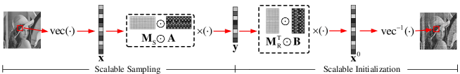
Figure 1: Scalable sampling and scalable initialization of an image block.

At present, there exist a few methods  [32, 30, 33, 34, 17] which reconstruct images at different CS ratios using only one model, and they can be roughly cast into two categories. The first kind [32, 30] trains a single model with a set of sampling matrices with different CS ratios so that the model can adapt to all sampling matrices in this set. The second kind [33, 34] applies only one sampling matrix in a learning way and integrates its rows to achieve sampling and reconstruction at different CS ratios, and we call such a strategy as scalable sampling and reconstruction (SSR) in this paper. And in this paper, we focus on SSR methods, because they are more practical in existing applications such as MRI [28], SPI [4] and wireless broadcasting [3], and it has been proved that the trained sampling matrix can improve the reconstruction performance [21, 9, 35]. However, existing SSR methods cannot be applied universally [33] or a more appropriate sampling matrix is needed [34]. Therefore, a general and more effective SSR method is expected.

In this paper, inspired by some methods [21, 9] which jointly train the sampling matrices with the models, we propose a general framework dubbed scalable deep compressive sensing (SDCS) to achieve sampling and reconstructing images at all CS ratios in a certain range. In detail, a trainable initialization matrix is designed to map measurements to their original shapes. And two binary sampling matrix masks are introduced to control the CS ratios for SSR. Most importantly, a novel training strategy named scalable training is developed to obtain an appropriate combination of sampling matrix and model, which performs well at all CS ratios in a certain range. We emphasize that SDCS can bring the model the ability of SSR, while maintaining the characteristics of its own structure. Furthermore, experimental results show that the model with SDCS can obtain a more effective combination of sampling matrix and model than existing SSR methods.

Our paper has three contributions:

• We propose a framework named SDCS that jointly trains the sampling matrix and the model to achieve sampling and reconstruction at all CS ratios in a certain range.

• With SDCS, a deep learning model can achieve SSR without changing its original structure, while maintaining good performance.

• Technically, SDCS can be used for all end-to-end-trained deep learning models.

The framework of the remaining content is as follows: Section II describes the proposed framework SDCS. Section III introduces some related works of this paper. Section IV is the experimental results. Section V concludes this paper.

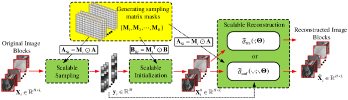
Figure 2: Forward-propogation of the scalable training.

II SDCS

In this section, we introduce the proposed framework SDCS which is simple but powerful. SDCS is composed of four parts: scalable sampling, scalable initialization, scalable reconstruction and scalable training.

II-A Scalable Sampling

Assume that the largest CS ratio is $R_{\text{M}}$, then the sampling matrix can be expressed as $\mathbf{A}\in{\mathbb{R}^{\left\lceil{{R_{\text{M}}}N}\right\rceil\times N}}$. It can be noticed that the CS ratio is determined by the row number of $\mathbf{A}$. Therefore, to achieve scalable sampling, we design a sampling matrix mask $\mathbf{M}_{\text{S}}\in{\mathbb{R}^{\left\lceil{{R_{\text{M}}}N}\right\rceil\times N}}$ to control the activities of the rows of $\mathbf{A}$. $\mathbf{M}_{\text{S}}$ is a zero-one matrix which satisfies $\mathbf{M}_{\text{S}}(1:\left\lceil{{R_{\text{S}}}N}\right\rceil,:)=1$ and $\mathbf{M}_{\text{S}}(\left\lceil{{R_{\text{S}}}N}\right\rceil+1:\left\lceil{{R_{\text{M}}}N}\right\rceil,:)=0$, where $R_{\text{S}}$ denotes the CS ratio for sampling. In such a case, we can generate a new sampling matrix as $\mathbf{A}_{\text{S}}=\mathbf{M}_{\text{S}}\odot\mathbf{A}$, where $\odot$ denotes the element-wise product. Since the $\left\lceil{{R_{\text{S}}}N}\right\rceil+1$-th row to the $\left\lceil{{R_{\text{M}}}N}\right\rceil$-th row of $\mathbf{A}_{\text{S}}$ are all filled with 0, we say that the first row to the $\left\lceil{{R_{\text{S}}}N}\right\rceil$-th row of $\mathbf{A}$ are activated. In detail, if the original image block is $\bar{\mathbf{X}}\in\mathbb{R}^{H\times L}$ satisfying $N=HL$, then the scalable sampling at the CS ratio of $R_{\text{S}}$ can be expressed as:

$${\mathbf{y}}=\mathbf{A}_{\text{S}}\operatorname{vec}({\bar{\mathbf{X}}}),$$ (2)

where $\operatorname{vec}(\cdot)$ is an operator which transforms a matrix to a vector and $\mathbf{y}\in{\mathbb{R}^{\left\lceil{{R_{\text{M}}}N}\right\rceil}}$ is the measurement. It can be noticed that $\mathbf{y}(\left\lceil{{R_{\text{S}}}N}\right\rceil+1:\left\lceil{{R_{\text{M}}}N}\right\rceil)=0$ and $\mathbf{y}(1:\left\lceil{{R_{\text{S}}}N}\right\rceil)$ is the valid measurement for reconstruction.

II-B Scalable Initialization

For deep learning methods, the initialized image is important in the following reconstruction. In SDCS, we use a linear operation to initialize the image block.

An initialization matrix $\mathbf{B}\in{\mathbb{R}^{N\times\left\lceil{{R_{\text{M}}}N}\right\rceil}}$ is developed. Similar to (2), a sampling matrix mask $\mathbf{M}_{\text{R}}\in{\mathbb{R}^{\left\lceil{{R_{\text{M}}}N}\right\rceil\times N}}$ is proposed to control the activities of the columns of $\mathbf{B}$, where $\mathbf{M}_{\text{R}}(1:\left\lceil{{R_{\text{R}}}N}\right\rceil,:)=1$ and $\mathbf{M}_{\text{R}}(\left\lceil{{R_{\text{R}}}N}\right\rceil+1:\left\lceil{{R_{\text{M}}}N}\right\rceil,:)=0$. $R_{\text{R}}$ denotes the CS ratio for initialization and reconstruction, which satisfies $R_{\text{R}}\leq R_{\text{S}}$. In such a case, we can activate the first column to the $\left\lceil{{R_{\text{R}}}N}\right\rceil$-th column of $\mathbf{B}$ to generate a new initialization matrix as $\mathbf{B}_{\text{R}}={\mathbf{M}_{\text{R}}}^{\operatorname{T}}\odot\mathbf{B}$. The detailed scalable initialization at the CS ratio of $R_{\text{R}}$ can be expressed as:

$$\mathbf{X}^{0}=\operatorname{vec}^{-1}(\mathbf{B}_{\text{R}}\mathbf{y}),$$ (3)

where $\mathbf{X}^{0}\in\mathbb{R}^{H\times L}$ denotes the initialized image block and $\operatorname{vec}^{-1}(\cdot)$ is the operator which transforms a vector to matrix.

In some cases, $R_{\text{R}}$ can be lower than $R_{\text{S}}$. For example, in wireless broadcasting [3], images are transferred at a high CS ratio and are received at a low CS ratio due to the poor channel condition. Fig. 1 illustrates the scalable sampling and scalable initialization of an image.

Algorithm 1 Scalable training of one epoch.

Input: training set $\mathbb{T}$, batch size $B$, max CS ratio $R_{\text{M}}$, sampling matrix $\mathbf{A}$, initialization matrix $\mathbf{B}$, reconstruction model $\mathfrak{F}_{\text{tra}}(\cdot;\mathbf{\Theta})$ or $\mathfrak{F}_{\text{unf}}(\cdot;\mathbf{A},\mathbf{\Theta})$.
  Output: trained parameters.

1:${\mathbb{T}}^{\prime}\leftarrow\emptyset$

2:repeat

3:     Select $\mathbb{S}=\{\mathbf{X}_{1},\mathbf{X}_{2},\cdots,\mathbf{X}_{B}\}$ $\in\mathbb{T}\setminus\mathbb{T}^{\prime}$.

4:     $\mathbb{T}^{\prime}\leftarrow\mathbb{T}^{\prime}\cup\mathbb{S}$.

5:     Generate $\{R_{1},R_{2},\cdots,R_{B}\}$ randomly, where $R_{i}\in[1,R_{\text{M}}]$.

6:     Generate $\{\mathbf{M}_{1},\mathbf{M}_{2},\cdots,\mathbf{M}_{B}\}$, where $\mathbf{M}_{i}(1:\left\lceil{R_{i}N}\right\rceil,:)=1$ and $\mathbf{M}_{i}(\left\lceil{R_{i}N}\right\rceil+1:\left\lceil{{R_{\text{M}}}N}\right\rceil,:)=0$.

7:     Generate $\mathbb{A}_{\text{S}}=\{\mathbf{A}_{\text{S}1},\mathbf{A}_{\text{S}2},\cdots,\mathbf{A}_{\text{S}B}\}$, $\mathbb{A}_{\text{R}}=\{\mathbf{A}_{\text{R}1},\mathbf{A}_{\text{R}2},\cdots,\mathbf{A}_{\text{R}B}\}$ and $\mathbb{B}_{\text{R}}=\{\mathbf{B}_{\text{R}1},\mathbf{B}_{\text{R}2},\cdots,\mathbf{B}_{\text{R}B}\}$, where $\mathbf{A}_{\text{S}i}=\mathbf{M}_{i}\odot\mathbf{A}$, $\mathbf{A}_{\text{R}i}=\mathbf{M}_{i}\odot\mathbf{A}$ and $\mathbf{B}_{\text{R}i}=\mathbf{M}^{\operatorname{T}}_{i}\odot\mathbf{B}$.

8:     for $i=1:B$ do

9:         $\mathbf{y}_{i}=\mathbf{A}_{\text{S}i}\operatorname{vec}(\mathbf{X}_{i})$

10:         $\mathbf{X}_{i}^{0}=\operatorname{vec}^{-1}(\mathbf{B}_{\text{R}i}\mathbf{y}_{i})$

11:         $\hat{\mathbf{X}}_{i}=\mathfrak{F}_{\text{tra}}(\mathbf{X}^{0}_{i};\mathbf{\Theta})$ or $\hat{\mathbf{X}}_{i}=\mathfrak{F}_{\text{unf}}(\mathbf{X}^{0}_{i},\mathbf{y}_{i};\mathbf{A}_{\text{R}i},\mathbf{\Theta})$      

12:     Compute loss $L$ using $\{\hat{\mathbf{X}}_{1},\hat{\mathbf{X}}_{2},\cdots,\hat{\mathbf{X}}_{B}\}$ and $\mathbb{S}$.

13:     Updating $\mathbf{A}$, $\mathbf{B}$ and $\mathbf{\Theta}$.

14:until $\mathbb{T}\setminus\mathbb{T}^{\prime}=\emptyset$

15:return $\mathbf{A}$, ${\mathbf{B}}$, $\mathbf{\Theta}$.

II-C Scalable Reconstruction

In this subsection, we describe the scalable reconstruction of two different kinds of deep learning models: traditional deep learning models and deep unfolding models.

The generalized reconstruction process of traditional deep learning models can be expressed as:

$${\hat{\mathbf{X}}}=\mathfrak{F}_{\text{tra}}(\mathbf{X}^{0};\mathbf{\Theta}),$$ (4)

where ${\hat{\mathbf{X}}}\in\mathbb{R}^{H\times L}$ is the reconstructed image block and $\mathbf{\Theta}$ contains trainable parameters of the model. In SDCS, $\mathbf{\Theta}$ is trained with $\mathbf{A}$ and $\mathbf{B}$ to make sure that $\mathfrak{F}_{\text{tra}}(\cdot;\mathbf{\Theta})$ can perform well at all CS ratios.

The reconstruction model of a deep unfolding model is usually composed of $K$ reconstruction modules with the same structure. In each module, the sampling matrix also participates in the image reconstruction. In detail, the generalized reconstruction process of a deep unfolding model can be expressed as:

$$\hat{\mathbf{X}} =\mathfrak{F}_{\text{unf}}(\mathbf{X^{0}},\mathbf{y};\mathbf{A},\mathbf{\Theta})=\mathfrak{F}_{\text{unf}}^{K}(\mathbf{X}^{K-1},\mathbf{y};\mathbf{A},\mathbf{\Theta}^{K}),$$ (5)

$$\mathbf{X}^{k} =\mathfrak{F}_{\text{unf}}^{k}(\mathbf{X}^{k-1},\mathbf{y};\mathbf{A},\mathbf{\Theta}^{k}),$$ (6)

where $\mathfrak{F}_{\text{unf}}(\cdot,\cdot;\mathbf{A},\mathbf{\Theta})$ is the entire deep unfolding model, of which $\mathbf{\Theta}$ contains its trainable parameters. $\mathfrak{F}_{\text{unf}}^{k}(\cdot,\cdot;\mathbf{A},\mathbf{\Theta}^{k})$ is the $k$-th reconstruction module and $\mathbf{\Theta}^{k}$ contains its trainable parameters. the inputs of $\mathfrak{F}_{\text{unf}}(\cdot,\cdot;\mathbf{A},\mathbf{\Theta})$ and $\mathfrak{F}_{\text{unf}}^{k}(\cdot,\cdot;\mathbf{A},\mathbf{\Theta}^{k})$ usually contain the image block $\mathbf{X}^{0}$ and the measurement $\mathbf{y}$. Since $\mathbf{A}$ plays an important role in each reconstruction module, the scalable reconstruction of the deep unfolding model is achieved by applying activated sampling matrix. In detail, the scalable reconstruction of the $k$-th reconstruction model can be expressed as:

$$\mathbf{X}^{k} =\mathfrak{F}_{\text{unf}}^{k}(\mathbf{X}^{k-1},\mathbf{y};{\mathbf{M}_{\text{R}}}\odot\mathbf{A},\mathbf{\Theta}^{k}).$$ (7)

Similar the traditional deep learning models, $\mathbf{\Theta}=\{\mathbf{\Theta}^{1},\mathbf{\Theta}^{2},\cdots,\mathbf{\Theta}^{K}\}$ is trained with $\mathbf{A}$ and $\mathbf{B}$. Since the sampling matrix $\mathbf{A}$ usually appears in the image sampling and reconstruction of deep unfolding models, deep unfolding models have a great potential to achieve SSR.

II-D Scalable Training

As shown in (2), (3) and (7), $\mathbf{A}$ and $\mathbf{B}$ are important in effective SSR. How to obtain an appropriate combination of $\mathbf{A}$, $\mathbf{B}$ and the reconstruction model is the main issue. To this end, we develop a novel training strategy dubbed scalable training to train $\mathbf{A}$, $\mathbf{B}$ with parameters of the reconstruction model jointly.

In scalable training, it is assumed that all parameters are trained using stochastic-gradient-descent-related algorithms like Adam [31]. If the batch size for training is $B$, the training process of $\mathbf{A}$, $\mathbf{B}$ and $\mathbf{\Theta}$ of one epoch can be expressed as Algorithm 1. And Fig. 2 illustrates the forward-propagation of the scalable training. The gradients of $\mathbf{A}$ and $\mathbf{B}$ can be computed as follows:

$${\nabla_{\mathbf{A}}}L=\frac{1}{B}\sum\limits_{i=1}^{B}{{{\mathbf{M}}_{i}}\odot}{\nabla_{{{\mathbf{M}}_{i}}\odot\mathbf{A}}}L,$$ (8)

$${\nabla_{\mathbf{B}}}L=\frac{1}{B}\sum\limits_{i=1}^{B}{{{\mathbf{M}}_{i}}^{\operatorname{T}}\odot}{\nabla_{{{\mathbf{M}}_{i}}^{\operatorname{T}}\odot\mathbf{B}}}L.$$ (9)

It can be noticed that the closer to the top of $\mathbf{A}$ or the left of $\mathbf{B}$, the more gradient information for updating is obtained, which makes using $\mathbf{M}_{\text{S}}$ and $\mathbf{M}_{\text{R}}$ for effective SSR possible.

Furthermore, to validate the trained model, a CS ratio validation group (RVG) is applied. Each RVG contains $G$ validation CS ratios as $\{{R_{1}},{R_{2}},\cdots,{R_{G}}\}$. At the end of each epoch, for each ratio $R_{i}$, the average PSNR on the validation set can be obtained. And the model with the best average PSNR on RVG is regarded as the model for test.

We emphasize that SDCS has no restriction on the structure of deep learning models, which means it can be combined with any end-to-end-trained model for SSR. However, the final performance is determined by the structure of the reconstruction model.

III Related Works

In this section, we first introduce some deep-learning-based methods for image CS, then some SSR methods are compared with SDCS.

III-A Deep Learning Models for Image CS

For traditional deep learning models, Mousavi et al. [20] first designed a fully-connected-layer-based stacked denoising autoencoder (SDA) for visual image CS. Lohit et al. [4] first proposed a six-layers CNN-based model named ReconNet to reconstruct image blocks from measurements. Shi et al. [21] proposed a deeper CNN model named CSNet which has trainable deblocking operations and integrated residual connection [24] for better performance. Furthermore, there are some other models [36, 37, 23, 38] for image CS, and all these models have one thing in common that the models for reconstruction are trained end-to-end.

Deep unfolding models are first developed for the sparse coding problem [27, 39, 40]. And inspired by these models, Zhang et al. [8] developed a deep unfolding model named ISTA-Net for image CS problem by unfolding ISTA and learning sparse transformation functions. Metzler et al. [26] and Zhang et al. [9] established deep unfolding models named LDAMP and AMP-Net respectively based on AMP algorithm, where LDAMP samples and reconstructs the entire image, and AMP-Net measures and recovers an image block-by-block with general trainable deblocking modules. Dong et al. [19] designed an model named DPDNN inspired by HQS algorithm for image inverse problem which can be applied for image CS. These deep unfolding models apply the sampling matrix for reconstruction and they can also be trained end-to-end.

Some of the above methods discuss the sampling matrix training strategies, including in traditional deep learning models [20, 21] or in deep unfolding model [9]. Although the trained sampling matrices can improve the reconstruction performance, they are designed for the single CS ratios and the performance would decrease seriously when the CS ratio changes for SSR. However, using SDCS, the model and the trained sampling matrix can perform well in all CS ratios in a certain range.

III-B SSR Methods

As far as we know, there exist two SSR methods [33, 34] for the visual image CS. Shi et al. [33] proposed a model dubbed SCSNet and Lohit et al. [34] designed a general framework named Rate-Adaptive CS (RACS). We compare them with SDCS in the following two paragraphs.

SCSNet trains the sampling matrix with the reconstruction model which is composed of seven independent sub-models with the same structure. Each sub-model adapts to a sub-range of CS ratios to make sure that the whole model can achieve SSR at CS ratios from 1% to 50%. And a greedy algorithm is applied to rearrange the rows of the sampling matrix for better reconstruction. However, SCSNet has two weaknesses: 1) The number of parameters is very large due to the existence of multiple sub-models. 2) Based on SCSNet, the existing deep learning models have to change their structure to achieve scalable reconstruction which would bring more burden to the hardware. However, SDCS needs only one model to achieve SSR and it can be applied for all end-to-end-trained models without changing their structures.

TABLE I: The results of twelve models tested on Set11 at different CS ratios, where the best is marked in bold.

Method	50$\%$	40$\%$	30$\%$	25$\%$	10$\%$	4$\%$	1$\%$
	PSNR (dB)/SSIM
SDA [20]	26.43/0.8007	25.14/0.7371	24.77/0.7191	24.77/0.7234	23.66/0.6794	21.05/0.5720	17.69/0.4376
SDA-SDCS	30.80/0.9038	30.63/0.9009	29.43/0.8793	28.76/0.8636	25.58/0.7660	22.77/0.6458	19.87/0.4829
ReconNet [4]	32.12/0.9137	30.59/0.8928	28.72/0.8517	28.04/0.8303	24.07/0.6958	21.00/0.5817	17.54/0.4426
ReconNet-SDCS	34.29/0.9532	33.81/0.9242	32.42/0.9313	31.42/0.9173	26.90/0.8225	23.57/0.6931	20.02/0.5071
${\text{CSNe}}{{\text{t}^{+}}}$ [21]	38.19/0.9739	36.15/0.9625	33.90/0.9449	32.76/0.9322	27.76/0.8513	24.24/0.7412	20.09/0.5334
${\text{CSNe}}{{\text{t}^{+}}}$-SDCS	36.65/0.9645	35.48/0.9568	33.58/0.9414	32.44/0.9295	27.85/0.8493	23.92/0.7303	20.32/0.5394
${\text{ISTA-Ne}}{{\text{t}}^{+}}$ [8]	38.08/0.9680	35.93/0.9537	33.66/0.9330	32.27/0.9167	25.93/0.7840	21.14/0.5947	17.48/0.4403
${\text{ISTA-Ne}}{{\text{t}}^{+}}$-SDCS	36.51/0.9693	34.92/0.9587	32.85/0.9400	31.65/0.9256	26.99/0.8334	23.57/0.7073	20.13/0.5146
DPDNN [19]	35.85/0.9532	34.30/0.9411	32.06/0.9145	30.63/0.8924	24.53/0.7392	21.11/0.6029	17.59/0.4459
DPDNN-SDCS	39.50/0.9775	37.61/0.9686	35.38/0.9543	34.12/0.9434	29.07/0.8708	25.08/0.7622	20.55/0.5423
AMP-Net [9]	40.27/0.9804	38.23/0.9713	35.90/0.9574	34.59/0.9477	29.45/0.8787	25.16/0.7692	20.57/0.5639
AMP-Net-SDCS	39.67/0.9781	37.96/0.9703	35.89/0.9576	34.67/0.9477	29.59/0.8792	25.43/0.7750	20.47/0.5629

TABLE II: The results of twelve models tested on the test set of BSDS500 at different CS ratios, where the best is marked in bold.

Method	50$\%$	40$\%$	30$\%$	25$\%$	10$\%$	4$\%$	1$\%$
	PSNR (dB)/SSIM
SDA [20]	26.16/0.8048	24.97/0.7392	24.58/0.7127	24.58/0.7107	23.77/0.6489	21.75/0.5534	19.05/0.4522
SDA-SDCS	30.17/0.9026	29.90/0.8973	28.77/0.8704	28.13/0.8510	25.43/0.7338	23.38/0.6145	21.08/0.4865
ReconNet [4]	30.85/0.8949	29.47/0.8647	27.95/0.8190	27.20/0.7914	23.98/0.6472	21.69/0.5557	18.96/0.4531
ReconNet-SDCS	33.27/0.9448	32.52/0.9355	31.04/0.9107	30.13/0.8921	26.46/0.7753	23.99/0.6502	21.20/0.5063
${\text{CSNe}}{{\text{t}^{+}}}$ [21]	35.89/0.9677	33.96/0.9513	31.94/0.9251	30.91/0.9067	27.01/0.7949	24.41/0.6747	21.42/0.5261
${\text{CSNe}}{{\text{t}^{+}}}$-SDCS	34.91/0.9588	33.59/0.9462	31.80/0.9221	30.82/0.9043	26.97/0.7906	24.21/0.6692	21.48/0.5288
${\text{ISTA-Ne}}{{\text{t}}^{+}}$ [8]	34.92/0.9510	32.87/0.9264	30.77/0.8901	29.64/0.8638	25.11/0.7124	21.82/0.5661	18.92/0.4529
${\text{ISTA-Ne}}{{\text{t}}^{+}}$-SDCS	34.85/0.9622	33.26/0.9465	31.38/0.9199	30.36/0.9003	26.56/0.7811	24.00/0.6555	21.24/0.5096
DPDNN [19]	33.56/0.9373	32.05/0.9164	29.98/0.8759	28.87/0.8491	24.37/0.6863	21.80/0.5716	18.97/0.4544
DPDNN-SDCS	36.84/0.9708	34.91/0.9560	32.85/0.9323	31.74/0.9150	27.58/0.8069	24.78/0.6858	21.72/0.5319
AMP-Net [9]	37.48/0.9744	35.34/0.9594	33.17/0.9358	32.01/0.9188	27.82/0.8133	24.95/0.6949	21.90/0.5501
AMP-Net-SDCS	37.04/0.9720	35.18/0.9580	33.14/0.9354	32.04/0.9187	27.84/0.8136	25.03/0.6967	21.87/0.5493

TABLE III: Parameter number of the reconstruction model of seven models.

Parameter	SDA-SDCS	ReconNet-SDCS	${\text{CSNe}}{{\text{t}^{+}}}$-SDCS	${\text{ISTA-Ne}}{{\text{t}}^{+}}$-SDCS	DPDNN-SDCS	AMP-Net-SDCS	SCSNet
Number	6534	22914	370560	336978	1363712	229254	1110823

RACS is a general framework like SDCS and it has three training stages. In the stage 1, the model is trained with the sampling matrix at a single CS ratio of $R_{\text{M}}$. And all parameters of the model are frozen after the stage 1. In the stage 2, The first $R_{\text{K}}N$ rows of the sampling matrix are optimized, where $R_{\text{K}}<R_{\text{M}}$. In the stage 3, the following rows of the sampling matrix are trained one-by-one. It can be noticed that RACS has an obvious weakness: the model is learned for a specific sampling matrix with CS ratio $R_{\text{M}}$ in the stage 1, which means the performance of the model at lower CS ratios can be further improved. Different from RACS, with SDCS, the learned model adapt to a sampling matrix which can change its CS ratios from 1% to $R_{\text{M}}$ using a sampling matrix mask. Our strategy brings the model the potential that performs better for SSR.

IV Experimental Results

IV-A Experimental settings

In this paper, the model combined with SDCS is named as model-SDCS. To evaluate the performance of SDCS, six models are combined with SDCS, namely SDA [20], ReconNet [4], ${\text{CSNe}}{{\text{t}^{+}}}$ [21], ${\text{ISTA-Ne}}{{\text{t}}^{+}}$ [8], DPDNN [19] and AMP-Net [9], which sample and reconstruct images block-by-block with the block size of $33\times 33$ that makes $N=1089$. SDA, ReconNet, ${\text{CSNe}}{{\text{t}^{+}}}$ are traditional deep learning models. ${\text{ISTA-Ne}}{{\text{t}}^{+}}$, DPDNN and AMP-Net are deep unfolding models with 9, 6 and 6 reconstruction modules respectively. In this paper, the activation fucntions of SDA are changed to the Rectified Linear Unit (ReLU) [4] for better performance. It is worth noting that in ${\text{CSNe}}{{\text{t}^{+}}}$ and AMP-Net, trainable deblocking operations are applied and the sampling matrices are trained for a single CS ratio. Furthermore, since SCSNet [33] and RACS [34] can achieve SSR like $model$-SDCS, they are compared with SDCS to show the effectiveness of our framework.

All of our experiments are performed on two datasets: BSDS500 [41] and Set11 [4]. BSDS500 contains 500 colorful visual images and is composed of a training set (200 images), a validation set (100 images) and a test set (200 images). Set11 [4] contains 11 grey-scale images. In this paper, BSDS500 is used for training, validation and testing. And Set11 is used for testing. We generate two training sets for models with and without trainable deblocking operations. (a) Training set 1 contains 89600 sub-images sized of $99\times 99$ which are randomly extracted from the luminance components of images in the training set of BSDS500  [21]. (b) Training set 2 contains 195200 sub-images sized of $33\times 33$ which are randomly extracted from the luminance components of images in the training set of BSDS500  [8]. In this paper ${\text{CSNe}}{{\text{t}^{+}}}$, AMP-Net, ${\text{CSNe}}{{\text{t}^{+}}}$-SDCS, AMP-Net-SDCS and SCSNet are trained on training set 1 due to the existence of trainable deblocking operations. SDA, ReconNet, ${\text{ISTA-Ne}}{{\text{t}}^{+}}$, DPDNN, SDA-SDCS, ReconNet-SDCS, ${\text{ISTA-Ne}}{{\text{t}}^{+}}$-SDCS and DPDNN-SDCS are trained on training set 2. And they are trained on the conditions in their original papers. Moreover, we use the validation set of BSDS500 for model choosing and the test set of BSDS500 for testing. In this paper, all sampling matrices are initialized randomly in Gaussian distribution. $R_{\text{M}}$ is 50% and RVG is $\{1\%,4\%,10\%,25\%,30\%,40\%,50\%\}$. All experiments are performed on a computer with an AMD Ryzen7 2700X CPU and an RTX2080Ti GPU.

IV-B Comparison with original deep learning methods

In this subsection, we compare SDA, ReconNet, ${\text{CSNe}}{{\text{t}^{+}}}$, ${\text{ISTA}}{{\text{-Net}^{+}}}$, DPDNN and AMP-Net with SDA-SDCS, ReconNet-SDCS, ${\text{CSNe}}{{\text{t}^{+}}}$-SDCS, ${\text{ISTA-Ne}}{{\text{t}}^{+}}$-SDCS, DPDNN-SDCS and AMP-Net-SDCS. Table I and Table II show the average PSNR and SSIM of 12 models tested on Set11 and the testing set of BSDS500 at different CS ratios respectively. We emphasize that there are seven different models for seven different test CS ratios for the method without SDCS, and a single model is tested at different CS ratios for $model$-SDCS.

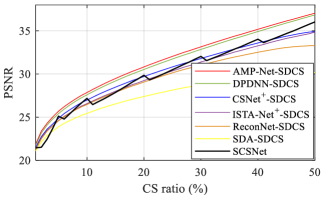
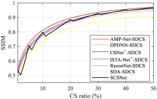
Figure 3: Comparison between SCSNet and six models with SDCS at different CS ratios.

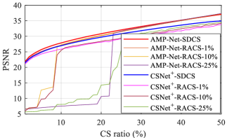
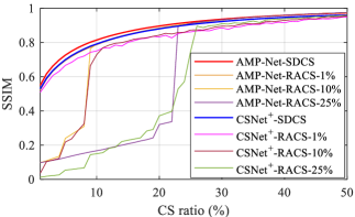
Figure 4: Comparison between SDCS and RACS at different CS ratios.

From Table I and Table II, it can be found that compared with models without trained sampling matrices, although $model$-SDCS has only one model for reconstruction, it obtains better performance in terms of PSNR and SSIM at most test CS ratios. And compared with models that apply trained sampling matrices, the average PSNR and SSIM of model-SDCS are not much different from them at most CS ratios and even higher than them at some CS ratios. Therefore, we conclude that $model$-SDCS can effectively achieve SSR without changing the structure of the model.

Furthermore, by further analyzing ${\text{CSNe}}{{\text{t}^{+}}}$, ${\text{CSNe}}{{\text{t}^{+}}}$-SDCS, AMP-Net and AMP-Net-SDCS, it can be noticed that even the sampling matrices of ${\text{CSNe}}{{\text{t}^{+}}}$ and AMP-Net are trained, ${\text{CSNe}}{{\text{t}^{+}}}$-SDCS and AMP-Net-SDCS can still obtain competitive performance at all test CS ratios with a single model. Such a result implies the great potential of deep leaning techniques and the sampling matrix training strategy.

IV-C Comparison with SSR methods

In this subsection, we compare SDCS with two SSR methods: SCSNet [33] and RACS [34].

First, SCSNet is compared with SDA-SDCS, ReconNet-SDCS, ${\text{CSNe}}{{\text{t}^{+}}}$-SDCS, ${\text{ISTA-Ne}}{{\text{t}}^{+}}$-SDCS, DPDNN-SDCS and AMP-Net-SDCS. Table III shows the parameter number of the seven models. Fig. 3 plots average PSNR and SSIM of the seven models tested on the test set of BSDS500 at CS ratios from 1% to 50%. It can be noticed that except DPDNN-SDCS, other models have fewer parameters than SCSNet and achieve SSR. And DPDNN-SDCS and AMP-Net-SDCS even outperform SCSNet, which shows the great potential of SDCS. Furthermore, deep unfolding models have better SSR performance than traditional deep learning models. For examples, AMP-Net-SDCS and DPDNN-SDCS outperform SDA-SDCS, ReconNet-SDCS and ${\text{CSNe}}{{\text{t}^{+}}}$-SDCS, and ${\text{ISTA-Ne}}{{\text{t}}^{+}}$-SDCS outperform SDA-SDCS and ReconNet-SDCS. we conclude that deep unfolding models are more suitable for SSR to a certain degree due to the important role of the sampling matrix in the image reconstruction process.

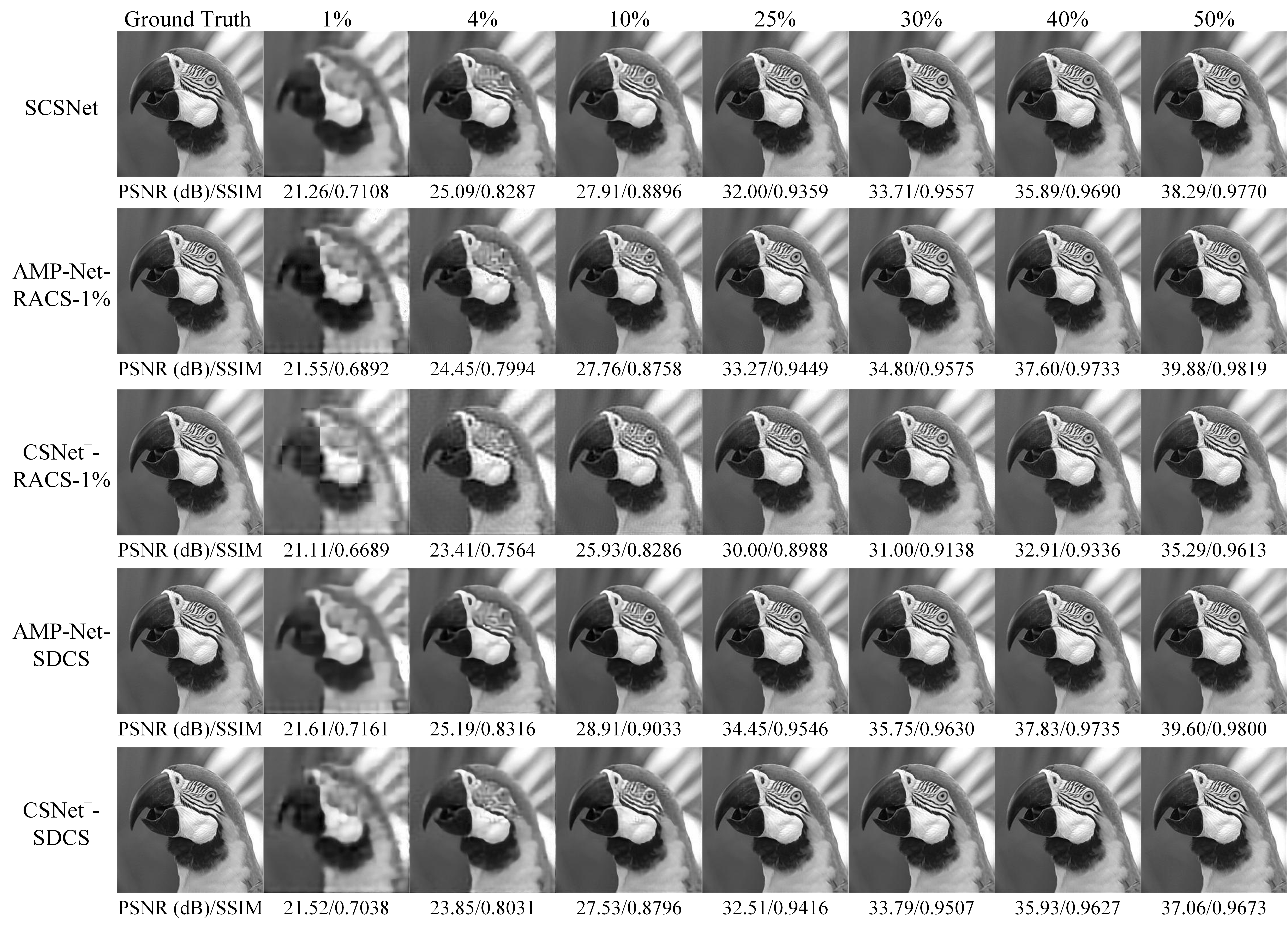
Figure 5: The Parrots images in Set11 Reconstructed by different SSR methods at different CS ratios.

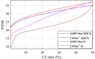
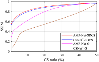
Figure 6: Comparison between two models with and without SDCS at different CS ratios. $model$-G is the model combined with the greegy algorithm in [33].

Second, SDCS is compared with RACS. Since with SDCS, AMP-Net outperforms other deep unfolding models and ${\text{CSNe}}{{\text{t}^{+}}}$ outperforms other traditional deep learning models, we use AMP-Net and ${\text{CSNe}}{{\text{t}^{+}}}$ as examples to compare SDCS and RACS. In this subsection, the values of $R_{\text{K}}$ of RACS mentioned in III-B are 1%, 10% and 25%. Fig. 4 plots average PSNR and SSIM of AMP-Net-SDCS, ${\text{CSNe}}{{\text{t}^{+}}}$-SDCS, AMP-Net-RACS-$R_{\text{K}}$ and ${\text{CSNe}}{{\text{t}^{+}}}$-RACS-$R_{\text{K}}$ on the test set of BSDS500 at CS ratios from 1% to 50%, where $model$-RACS-$R_{\text{K}}$ denotes the model combined with RACS with the hyperparameter $R_{\text{K}}$. It can be noticed that when the CS ratio is lower than $R_{\text{K}}$, $model$-RACS-$R_{\text{K}}$ has bad performance. For AMP-Net, AMP-Net-SDCS outperforms all compared AMP-Net-RACS-$R_{\text{K}}$s when the CS ratio is lower than 30%. And for ${\text{CSNe}}{{\text{t}^{+}}}$, ${\text{CSNe}}{{\text{t}^{+}}}$-SDCS has better performance than all compared ${\text{CSNe}}{{\text{t}^{+}}}$-RACS-$R_{\text{K}}$s at all CS ratios. Such a result implies that SDCS can generate a more appropriate combination of sampling matrix and model than RACS.

Fig. 5 shows the Parrots images in Set11 reconstructed by different SSR models at different CS ratios. Fig. 5 is quite revealing in several ways. 1) AMP-Net-SDCS generates better results than SCSNet while maintaining fewer parameters which shows the great potential of SDCS. 2) $Model$-RACS-$R_{\text{K}}$ can not inherit the characteristics of original models well. For example, AMP-Net and CSNe${\text{t}}^{+}$ both have trainable deblocking operations, but AMP-Net-RACS-1% and CSNe${\text{t}}^{+}$-RACS-1% generates images with obvious blocking artifacts at CS ratios of 1%, 4% and 10%. However, AMP-Net-SDCS and CSNe${\text{t}}^{+}$-SDCS generate smooth images without blocking artifacts. Therefore, we conclude that models with SDCS can get good SSR performance. In particular, they can inherit the characteristics of original models.

To further prove the effectiveness of SDCS, we compare AMP-Net-SDCS and ${\text{CSNe}}{{\text{t}^{+}}}$-SDCS with AMP-Net and ${\text{CSNe}}{{\text{t}^{+}}}$ which train their sampling matrices for the single CS ratio. In this subsection, the sampling matrices of AMP-Net and ${\text{CSNe}}{{\text{t}^{+}}}$ are trained for the CS ratio of 50%. And their rows are rearranged using the greedy algorithm in SCSNet [33] for better SSR. Fig. 6 plots the average PSNR and SSIM of four models tested on the test set of BSDS500 at CS ratios from 1% to 50%. It can be noticed that at the CS ratio of 50%, the specially trained models can obtain better results than the models with SDCS, but such models have a bad performance at other CS ratios. However, models combined with SDCS perform well at all CS ratios. Therefore, we conclude that compared with methods that jointly train the sampling matrix and the model for a single CS ratio, $model$-SDCS can get better SSR performance.

V Conclusion

In this paper, for the visual image CS problem, we propose a general framework named SDCS to achieve sampling and reconstructing images using one sampling matrix and one deep learning model at different CS ratios. Theoretically, SDCS can be combined with all end-to-end-trained deep learning models which do not need to change their structures. Experimental results show that models with SDCS inherit the characteristics of the original models and perform well at all CS ratios in a certain range. And we further prove that SDCS outperforms other SSR methods. Finally, we highlight that SDCS can be also applied in other CS-based applications like video CS [22] and MRI [28].

References

- [1] M. F. Duarte, M. A. Davenport, D. Takhar, J. N. Laska, T. Sun, K. F. Kelly, and R. G. Baraniuk, “Single-pixel imaging via compressive sampling,” IEEE Signal Processing Magazine, vol. 25, no. 2, pp. 83–91, 2008.
- [2] Y. Liu, S. Wu, X. Huang, B. Chen, and C. Zhu, “Hybrid CS-DMRI : Periodic time-variant subsampling and omnidirectional total variation based reconstruction,” IEEE Transactions on Medical Imaging, vol. 36, no. 10, pp. 2148–2159, 2017.
- [3] W. Yin, X. Fan, Y. Shi, R. Xiong, and D. Zhao, “Compressive sensing based soft video broadcast using spatial and temporal sparsity,” Mobile Networks and Applications, vol. 21, no. 6, pp. 1002–1012, 2016.
- [4] S. Lohit, K. Kulkarni, R. Kerviche, P. Turaga, and A. Ashok, “Convolutional neural networks for noniterative reconstruction of compressively sensed images,” IEEE Transactions on Computational Imaging, vol. 4, no. 3, pp. 326–340, 2018.
- [5] C. Li, H. Jiang, P. Wilford, Y. Zhang, and M. Scheutzow, “A new compressive video sensing framework for mobile broadcast,” IEEE Transactions on Broadcasting, vol. 59, no. 1, pp. 197–205, 2013.
- [6] W. Dong, G. Shi, X. Li, Y. Ma, and F. Huang, “Compressive sensing via nonlocal low-rank regularization,” IEEE Transactions on Image Processing, vol. 23, no. 8, pp. 3618–3632, 2014.
- [7] K. Q. Dinh and B. Jeon, “Iterative weighted recovery for block-based compressive sensing of image/video at a low subrate,” IEEE Transactions on Circuits and Systems for Video Technology, vol. 27, no. 11, pp. 2294–2308, 2017.
- [8] J. Zhang and B. Ghanem, “ ISTA-Net : Interpretable optimization-inspired deep network for image compressive sensing,” in The IEEE Conference on Computer Vision and Pattern Recognition, 2018, pp. 1828–1837.
- [9] Z. Zhang, Y. Liu, J. Liu, F. Wen, and C. Zhu, “Amp-net: Denoising-based deep unfolding for compressive image sensing,” IEEE Transactions on Image Processing, vol. 30, pp. 1487–1500, 2021.
- [10] S. Mallat, A wavelet tour of signal processing. Elsevier, 1999.
- [11] M. Elad, Sparse and redundant representations: from theory to applications in signal and image processing. Springer Science & Business Media, 2010.
- [12] Y. Liu, Z. Long, H. Huang, and C. Zhu, “Low CP rank and Tucker rank tensor completion for estimating missing components in image data,” IEEE Transactions on Circuits and Systems for Video Technology, 2019.
- [13] C. A. Metzler, A. Maleki, and R. G. Baraniuk, “From denoising to compressed sensing,” IEEE Transactions on Information Theory, vol. 62, no. 9, pp. 5117–5144, 2016.
- [14] Y. Wu, M. Rosca, and T. Lillicrap, “Deep compressed sensing,” in The Thirty-sixth International Conference on Machine Learning (ICML 2019), 2019.
- [15] A. Beck and M. Teboulle, “A fast iterative shrinkage-thresholding algorithm for linear inverse problems,” SIAM Journal on Imaging Sciences, vol. 2, no. 1, pp. 183–202, 2009.
- [16] D. L. Donoho, A. Maleki, and A. Montanari, “Message-passing algorithms for compressed sensing,” Proceedings of the National Academy of Sciences, vol. 106, no. 45, pp. 18 914–18 919, 2009.
- [17] Y. Li, W. Dai, J. Zhou, H. Xiong, and Y. F. Zheng, “Scalable structured compressive video sampling with hierarchical subspace learning,” IEEE Transactions on Circuits and Systems for Video Technology, vol. 30, no. 10, pp. 3528–3543, 2020.
- [18] J. Rick Chang, C.-L. Li, B. Poczos, B. Vijaya Kumar, and A. C. Sankaranarayanan, “One network to solve them all–solving linear inverse problems using deep projection models,” in Proceedings of the IEEE International Conference on Computer Vision, 2017, pp. 5888–5897.
- [19] W. Dong, P. Wang, W. Yin, G. Shi, F. Wu, and X. Lu, “Denoising prior driven deep neural network for image restoration,” IEEE Transactions on Pattern Analysis and Machine Intelligence, vol. 41, no. 10, pp. 2305–2318, 2018.
- [20] A. Mousavi, A. B. Patel, and R. G. Baraniuk, “A deep learning approach to structured signal recovery,” in The 53rd Annual Allerton Conference on Communication, Control, and Computing. IEEE, 2015, pp. 1336–1343.
- [21] W. Shi, F. Jiang, S. Liu, and D. Zhao, “Image compressed sensing using convolutional neural network,” IEEE Transactions on Image Processing, vol. 29, pp. 375–388, 2019.
- [22] W. Shi, S. Liu, F. Jiang, and D. Zhao, “Video compressed sensing using a convolutional neural network,” IEEE Transactions on Circuits and Systems for Video Technology, pp. 1–1, 2020.
- [23] A. Bora, A. Jalal, E. Price, and A. G. Dimakis, “Compressed sensing using generative models,” in Proceedings of the 34th International Conference on Machine Learning, ser. Proceedings of Machine Learning Research, D. Precup and Y. W. Teh, Eds., vol. 70. International Convention Centre, Sydney, Australia: PMLR, 06–11 Aug 2017, pp. 537–546.
- [24] K. He, X. Zhang, S. Ren, and J. Sun, “Deep residual learning for image recognition,” in The IEEE Conference on Computer Vision and Pattern Recognition, 2016, pp. 770–778.
- [25] Y. Huang, T. Würfl, K. Breininger, L. Liu, G. Lauritsch, and A. Maier, “Some investigations on robustness of deep learning in limited angle tomography,” in International Conference on Medical Image Computing and Computer-Assisted Intervention. Springer, 2018, pp. 145–153.
- [26] C. Metzler, A. Mousavi, and R. Baraniuk, “Learned d-amp: Principled neural network based compressive image recovery,” in Advances in Neural Information Processing Systems, 2017, pp. 1772–1783.
- [27] K. Gregor and Y. LeCun, “Learning fast approximations of sparse coding,” in The 27th International Conference on International Conference on Machine Learning. Omnipress, 2010, pp. 399–406.
- [28] J. Sun, H. Li, Z. Xu et al., “Deep ADMM-Net for compressive sensing MRI ,” in Advances in Neural Information Processing Systems, 2016, pp. 10–18.
- [29] J. Ma, X.-Y. Liu, Z. Shou, and X. Yuan, “Deep tensor ADMM-Net for snapshot compressive imaging,” in Proceedings of the IEEE International Conference on Computer Vision, 2019, pp. 10 223–10 232.
- [30] Y. Su and Q. Lian, “ipiano-net: Nonconvex optimization inspired multi-scale reconstruction network for compressed sensing,” Signal Processing: Image Communication, vol. 89, 2020.
- [31] D. P. Kingma and J. Ba, “ ADAM : A method for stochastic optimization,” International Conference on Learning Representations, 2015.
- [32] Y. Xu, W. Liu, and K. F. Kelly, “Compressed domain image classification using a dynamic-rate neural network,” IEEE Access, vol. 8, pp. 217 711–217 722, 2020.
- [33] W. Shi, F. Jiang, S. Liu, and D. Zhao, “Scalable convolutional neural network for image compressed sensing,” in The IEEE Conference on Computer Vision and Pattern Recognition, 2019, pp. 12 290–12 299.
- [34] S. Lohit, R. Singh, K. Kulkarni, and P. Turaga, “Rate-adaptive neural networks for spatial multiplexers,” arXiv preprint arXiv:1809.02850, 2018.
- [35] M. Iliadis, L. Spinoulas, and A. K. Katsaggelos, “Deepbinarymask: Learning a binary mask for video compressive sensing,” Digital Signal Processing, vol. 96, p. 102591, 2020.
- [36] J. Du, X. Xie, C. Wang, G. Shi, X. Xu, and Y. Wang, “Fully convolutional measurement network for compressive sensing image reconstruction,” Neurocomputing, vol. 328, pp. 105–112, 2019.
- [37] H. Yao, F. Dai, S. Zhang, Y. Zhang, Q. Tian, and C. Xu, “Dr2-net: Deep residual reconstruction network for image compressive sensing,” Neurocomputing, vol. 359, pp. 483–493, 2019.
- [38] Y. Sun, J. Chen, Q. Liu, and G. Liu, “Learning image compressed sensing with sub-pixel convolutional generative adversarial network,” Pattern Recognition, vol. 98, p. 107051, 2020.
- [39] X. Chen, J. Liu, Z. Wang, and W. Yin, “Theoretical linear convergence of unfolded ISTA and its practical weights and thresholds,” in Advances in Neural Information Processing Systems, 2018, pp. 9061–9071.
- [40] M. Borgerding, P. Schniter, and S. Rangan, “ AMP-inspired deep networks for sparse linear inverse problems,” IEEE Transactions on Signal Processing, vol. 65, no. 16, pp. 4293–4308, 2017.
- [41] P. Arbelaez, M. Maire, C. Fowlkes, and J. Malik, “Contour detection and hierarchical image segmentation,” IEEE Transactions on Pattern Analysis and Machine Intelligence, vol. 33, no. 5, pp. 898–916, 2010.