Recently, an indicative evidence of a stochastic process, reported by the NANOGrav Collaboration based on the analysis of 12.5-year pulsar timing array data which might be interpreted as a potential stochastic gravitational wave signal, has aroused keen interest of theorists. The first-order color charge confinement phase transition at the QCD scale could be one of the cosmological sources for the NANOGrav signal. If the phase transition is flavor dependent and happens sequentially, it is important to find that what kind of QCD matter in which the first-order confinement/deconfinement phase transition happens is more likely to be the potential source of the NANOGrav signal during the evolution of the universe. In this paper, we would like to illustrate that the NANOGrav signal could be generated from confinement/deconfinement transition in either heavy static quarks with a zero baryon chemical potential, or quarks with a finite baryon chemical potential. In contrast, the gluon confinement could not possibly be the source for the NANOGrav signal according to the current observation. Future observation will help to distinguish between different scenarios.

shoulongli@hunnu.edu.cn   lshao@pku.edu.cn    pxwu@hunnu.edu.cn    hwyu@hunnu.edu.cn

1 Introduction

Recently, the North American Nanohertz Observatory for Gravitational Wave (NANOGrav) Collaboration [1] has reported an analysis of 12.5-year pulsar timing array (PTA) data. According to the analysis [1], a possible evidence is found for a stochastic common-spectrum process which may be interpreted as a gravitational wave (GW) signal with its frequency in $1$–$10$ nHz, and its average GW energy density $\langle\Omega_{\textup{GW}}h^{2}\rangle_{\textup{NANOGrav}}\sim 10^{-10}$ with an almost flat GW spectrum $\Omega_{\rm GW}h^{2}\sim f^{-1.5\pm 0.5}$ at 1-$\sigma$ level. Although the observational results need further analyses, such as a joint analysis with data from the other PTA collaborations (such as EPTA and PPTA) [2, 3, 4], the potentiality of its being a stochastic GW background (SGWB) signal has aroused keen interest of theorists [5, 6, 7, 8, 9, 10, 11, 12, 13, 14, 15, 16, 17, 18, 19, 20, 21, 22, 23, 24, 25, 26, 27, 28, 29, 30, 31, 32]. On the one hand, one may explain it as a potential SGWB signal by considering different astrophysical and cosmological sources. On the other hand, the possible SGWB signal could serve as a potential new probe to studying new physics.

During the evolution of the universe, as the temperature decreases, the universe may undergo several phase transitions from the metastable vacuums to stable vacuums. At the quantum chromodynamics (QCD) energy scale, there are two important transitions, i.e. the spontaneous chiral symmetry breaking and the color charge confinement. For the confinement transition, the universe will go from a quark-gluon plasma (QGP) phase to a hadron phase as the temperature decreases. The numerical lattice simulation shows [33, 34, 35] that the QCD transition is likely a crossover for three dynamical quark flavors when the baryon and charge chemical potential is negligible, i.e., in the absence of the baryon and lepton asymmetries. If the transition is first-order, GWs could be produced due to the violent process of vacuum bubble nucleation and subsequent bubble collisions [36, 42, 37, 38, 39, 40, 41], sound waves [43, 44, 45, 46] and magnetohydrodynamic (MHD) turbulence [47, 48, 49, 50, 51, 52, 53]. The GWs produced are within the frequency range of the PTA observation [54, 55, 56]. The three processes in the first-order phase transition could be potential sources of the NANOGrav signal [19, 17, 22]. Therefore, the next issue is what are the QCD matters in which the first-order phase transition can occur. In this regard, let us note that for the case of a zero baryon chemical potential, the transition is first-order in a non-dynamical (static) heavy quark system [57, 58]. For the case of a finite baryon chemical potential, a large lepton asymmetry might affect the dynamics of the QCD phase transition in a way to render it first-order in the early universe [59]. Besides, for a pure gluon system, the first-order phase transition might occur as well.

Different QCD matter has a different temperature of phase transition which is a crucial parameter determining the features of the GWs produced. Then a question arises naturally as to what kind of QCD matter in which the first-order confinement/deconfinement phase transition happens is more likely to be the potential source of the NANOGrav signal during the evolution of the universe. In this paper, we will try to answer this question. We consider three types of QCD matter systems: (i) heavy static quarks with a zero baryon chemical potential, (ii) quarks with a finite baryon chemical potential, and (iii) a pure gluon system. We match the NANOGrav signal with the GW spectra from the first-order confinement/deconfinement phase transitions in three QCD matter systems with holographic models [56, 60, 61]. We show that the GW spectra from the phase transitions in pure quark systems, regardless of whether the chemical potential is finite or zero, could explain the NANOGrav signal according to the current observation. In contrast, the signal could not possibly come from the gluon confinement.

2 GWs from first-order phase transitions

When first-order phase transition occurs, the universe transfers from a metastable vacuum to a stable vacuum. This process can be described as bubble nucleation. Generally, the GW signal from cosmological first-order phase transitions mainly comes from three processes: collisions of vacuum bubble walls, sound waves, and the MHD turbulence in the plasma [36, 42, 37, 38, 39, 40, 41, 43, 44, 45, 46, 47, 48, 49, 50, 51, 52, 53]. So, the total energy density of the GW, which is a sum of the three, is given by

$$h^{2}\Omega(f)\simeq h^{2}\Omega_{\textup{en}}(f)+h^{2}\Omega_{\textup{sw}}(f)+h^{2}\Omega_{\textup{tu}}(f)\,,$$ (2.1)

where $h=H_{0}/100\ \textup{km}^{-1}\ \textup{s}\ \textup{Mpc}$ in which $H_{0}$ is the Hubble constant today. $h^{2}\Omega_{\textup{en}}$, $h^{2}\Omega_{\textup{sw}}$ and $h^{2}\Omega_{\textup{tu}}$ are the contributions from bubble collision, sound waves, and the turbulence, respectively, which are given by [41, 42, 46, 52]

$$h^{2}\Omega_{\textup{en}} = 3.6\times 10^{-5}\left(\frac{H_{\ast}}{\beta}\right)^{2}\left(\frac{\kappa_{1}\alpha}{1+\alpha}\right)^{2}\left(\frac{10}{g_{\ast}}\right)^{\frac{1}{3}}\left(\frac{0.11v_{w}^{3}}{0.42+v_{w}^{2}}\right)S_{\textup{en}}\,,$$

$$h^{2}\Omega_{\textup{sw}} = 5.7\times 10^{-6}\left(\frac{H_{\ast}}{\beta}\right)\left(\frac{\kappa_{2}\alpha}{1+\alpha}\right)^{2}\left(\frac{10}{g_{\ast}}\right)^{\frac{1}{3}}v_{w}S_{\textup{sw}}\,,$$

$$h^{2}\Omega_{\textup{tu}} = 7.2\times 10^{-4}\left(\frac{H_{\ast}}{\beta}\right)\left(\frac{\kappa_{3}\alpha}{1+\alpha}\right)^{2}\left(\frac{10}{g_{\ast}}\right)^{\frac{1}{3}}v_{w}S_{\textup{tu}}\,.$$ (2.2)

In above equations, $\beta$ is the inverse time duration of the phase transition, $v_{w}$ is the velocity of bubble wall, $g_{\ast}$ and $H_{\ast}$ represent the number of active degrees of freedom and Hubble parameter at the time of production of GWs respectively, $\alpha=30\epsilon_{\ast}/(\pi^{2}g_{\ast}T_{\ast}^{4})$ is the ratio of the vacuum energy density $\epsilon_{\ast}=\big{[}\Delta F(T)-Td\Delta F(T)/dT\big{]}\Big{|}_{T=T_{\ast}}$ over radiation energy density where $T_{\ast}$ and $\Delta F(T)$ are the temperature of the thermal bath at time of production of GWs and the difference of the free energy between two phases respectively, and $S_{\textup{en}},S_{\textup{sw}}$, and $S_{\textup{tu}}$ are spectral shapes of GWs which are characterized from numerical fits as [41, 42, 46, 52]

$$S_{\textup{en}} = \frac{3.8\left(\frac{f}{f_{\textup{en}}}\right)^{2.8}}{1+2.8\left(\frac{f}{f_{\textup{en}}}\right)^{3.8}}\,,$$

$$S_{\textup{sw}} = \left(\frac{f}{f_{\textup{sw}}}\right)^{3}\left(\frac{7}{4+3\left(\frac{f}{f_{\textup{sw}}}\right)^{2}}\right)^{\frac{7}{2}}\,,$$

$$S_{\textup{tu}} = \frac{\left(\frac{f}{f_{\textup{tu}}}\right)^{3}}{\left(1+\frac{f}{f_{\textup{tu}}}\right)^{\frac{11}{3}}\left(1+\frac{8\pi f}{h_{\ast}}\right)}\,,$$ (2.3)

where $h_{\ast}$ is Hubble rate at $T_{\ast}$, $f_{\textup{en}},f_{\textup{sw}}$ and $f_{\textup{tu}}$ are peak frequencies in three cases, which are given by [39, 42, 52]

$$h_{\ast} = 11.2\ \textup{nHz}\ \left(\frac{T_{\ast}}{100\textup{MeV}}\right)\left(\frac{g_{\ast}}{10}\right)^{\frac{1}{6}}\,,$$

$$f_{\textup{en}} = 11.2\ \textup{nHz}\ \left(\frac{0.62}{1.8-0.1v_{w}+v_{w}^{2}}\right)\left(\frac{\beta}{H_{\ast}}\right)\left(\frac{T_{\ast}}{100\textup{MeV}}\right)\left(\frac{g_{\ast}}{10}\right)^{\frac{1}{6}}\,,$$

$$f_{\textup{sw}} = 12.9\ \textup{nHz}\ \left(\frac{1}{v_{w}}\right)\left(\frac{\beta}{H_{\ast}}\right)\left(\frac{T_{\ast}}{100\textup{MeV}}\right)\left(\frac{g_{\ast}}{10}\right)^{\frac{1}{6}}\,,$$

$$f_{\textup{tu}} = 18.4\ \textup{nHz}\ \left(\frac{1}{v_{w}}\right)\left(\frac{\beta}{H_{\ast}}\right)\left(\frac{T_{\ast}}{100\textup{MeV}}\right)\left(\frac{g_{\ast}}{10}\right)^{\frac{1}{6}}\,.$$ (2.4)

In Eq. (2.2), $\kappa_{1},\kappa_{2}$, and $\kappa_{3}$ are the fractions of the vacuum energy converted to the kinetic energy of the bubbles, bulk fluid motion, and the MHD turbulence, respectively. These factors are model-dependent. In this work, we consider two cases of bubble: Jouguet detonations and non-runaway bubbles. For the case of Jouguet detonations [62, 42, 39, 63, 64, 46], we have

$$\kappa_{1} = \frac{0.715\alpha+0.181\sqrt{\alpha}}{1+0.715\alpha}\,,$$

$$\kappa_{2} = \frac{\sqrt{\alpha}}{0.135+\sqrt{\alpha+0.98}}\,,$$

$$\kappa_{3} = 0.05\kappa_{2}\,,$$

$$v_{w} = \frac{\sqrt{1/3}+\sqrt{\alpha^{2}+2\alpha/3}}{1+\alpha}\,,$$ (2.5)

and for the case of non-runaway bubbles [64, 42, 46, 39],

$$\kappa_{1} = 0\,,$$

$$\kappa_{2} = \frac{\alpha}{0.73+0.083\sqrt{\alpha}+\alpha}\,,$$

$$\kappa_{3} = 0.05\kappa_{2}\,,$$

$$v_{w} = 0.95\,.$$ (2.6)

With all these expressions, there are still four unknown parameters in Eq. (2.1), i.e., $g_{\ast},\beta/H_{\ast}$, $T_{\ast}$ and $\alpha$, which characterize the first-order cosmological QCD phase transition. Generally, for QCD phase transitions, the temperature $T_{\ast}$ is around several hundreds MeV, of which the concrete value depends on the types of the QCD matter and the phase transition. We will obtain, in the following section, $T_{\ast}$ for the phase transition in different QCD matters by the method of the holographic QCD. One can also calculate $\alpha$ from different holographic models. For simplicity, we assume that the GW can be generated soon after the confinement/deconfinement phase transition occurs, so $T_{\ast}$ is approximated by the critical temperature of the phase transition. Besides, we fix $g_{\ast}$ and $\beta/H_{\ast}$ at their typical values which could be chosen as $g_{\ast}=10$ and $\beta/H_{\ast}=10$ [56, 60, 61] at the QCD scale.

3 GWs from holographic QCD models and the NANOGrav signal

In this section, we will obtain the GW spectra from the first-order confinement/deconfinement transition in heavy static quarks with a zero baryon chemical potential, quarks with a finite baryon chemical potential, and a pure gluon system, and match them with the NANOGrav signal. First, we start with finding the corresponding critical temperatures by use of holographic QCD models.

Following the Anti-de Sitter/conformal field theory (AdS/CFT) correspondence principle [65, 66, 67], AdS/QCD offers some new insights to the non-perturbative hadron dynamics from the dual gravitational field [68]. Especially, the first-order confinement/deconfinement phase transitions could be interpreted by Hawking-Page (HP) phase transitions [69] in five-dimensional spacetime in the AdS/QCD models [70], where the high-temperature QGP corresponds to the AdS black hole, while the low-temperature hadron corresponds to the thermal AdS space. In the absence of the baryon chemical potential, the transition temperature calculated by the soft-wall model is consistent with numerical results [70]. In the case of the finite baryon chemical potential, AdS/QCD models can also give a good explanation of the phase transition [71, 72, 73, 74], while the standard lattice QCD simulation suffers from the famous sign problem [75, 76, 77] and could not provide many useful results. The GW produced by the first-order QCD phase transition was estimated in the case of the heavy static quark system with a zero baryon chemical potential via hard-wall and soft-wall models of AdS/QCD in Ref. [56] for the first time, and then studied in the finite chemical potential system [60, 78] and pure gluon system [61] via different models. It is also worth mentioning that the initial idea of explaining GWs generated from cosmological phase transitions by holographic method could be traced back to Randall and Servant’s seminal work [79] in 2006 to the best of our knowledge.

We consider three types of QCD matter systems in five different holographic models: (i) heavy static quarks with a zero baryon chemical potential in hard-wall model $S_{1}$ and (ii) soft-wall model $S_{2}$, (iii) quarks with a finite baryon chemical potential in hard-wall model $S_{3}$ and (iv) soft-wall model $S_{4}$, and (v) pure gluons in the quenched dynamical holographic model $S_{5}$. The corresponding five-dimensional gravitational actions are given by [70, 60, 56, 61]

$$S_{1} = \frac{1}{2\kappa^{2}}\int d^{5}x\sqrt{-g}\left(R+\frac{12}{\ell^{2}}\right)\,,$$ (3.1)

$$S_{2} = \frac{1}{2\kappa^{2}}\int d^{5}x\sqrt{-g}e^{-\phi}\left(R+\frac{12}{\ell^{2}}\right)\,,$$ (3.2)

$$S_{3} = \int d^{5}x\sqrt{-g}\left[\frac{1}{2\kappa^{2}}\left(R+\frac{12}{\ell^{2}}\right)-\frac{1}{4g_{5}^{2}}F^{2}\right]-\frac{1}{\kappa^{2}}\int d^{4}x\sqrt{h}\nabla_{\mu}n^{\mu}\,,$$ (3.3)

$$S_{4} = \frac{1}{2\kappa^{2}}\int d^{5}x\sqrt{-g}e^{-\phi}\left[\frac{1}{2\kappa^{2}}\left(R+\frac{12}{\ell^{2}}\right)-\frac{1}{4g_{5}^{2}}F^{2}\right]-\frac{1}{\kappa^{2}}\int d^{4}x\sqrt{h}e^{-\phi}\nabla_{\mu}n^{\mu}\,,$$ (3.4)

$$S_{5} = \frac{1}{2\kappa^{2}}\int d^{5}x\sqrt{-g}e^{-2\varphi}\left(R-\frac{4}{3}\partial_{\mu}\varphi\partial^{\mu}\varphi-V(\varphi)\right)\,,$$ (3.5)

where $\kappa^{2}=8\pi G$, $g_{5}$ is coupling constant, $\ell$ is the radius of five-dimensional AdS space, $g$ and $h$ are determinants of bulk and boundary metrics respectively, $n^{\mu}$ is the unit vector normal to the hypersurface, $\phi$ is a non-dynamical dilaton, and $\varphi$ is a dynamical dilaton. The confinement/deconfinement transition in the cases of heavy static quarks with a zero baryon chemical potential and pure gluons are analogous to the HP transition between the static AdS black hole and the thermal AdS vacuum. For the case of quarks with a finite baryon chemical potential, the confinement/deconfinement transition is analogous to the HP transition between the charged AdS black hole and the thermal charged AdS vacuum, and the chemical potential is related to the electric charge of the black hole. For a specific model, one can calculate the free energies of the black hole and AdS vacuum respectively, and obtain the difference of the free energy $\Delta F$ between two phases. Then one can obtain the value of the temperature $T_{\ast}$ and $\alpha$ via some holographic techniques. Here, we refer readers to Refs. [70, 60, 56, 61] for detailed calculations and list the corresponding critical temperatures in these models in Table 1.

Table 1: Critical temperatures from five holographical QCD models.

QCD matters	Holographic QCD models	Temperature
heavy static quarks with	hard wall	122 MeV  [70, 56]
a zero chemical potential	soft wall	191 MeV [70, 56]
quarks with a finite	hard wall	112 MeV [60]
chemical potential	soft wall	192 MeV [60]
pure gluons	quenched dynamical holographic QCD	255 MeV [61]

We assume that GW is generated quickly after the phase transition occurs and temperature $T_{\ast}$ is approximated as the critical phase transition temperature. Now we match the NANOGrav results with the GW produced from the confinement/deconfinement phase transition in different holographic models. We plot the GW spectra in two bubble models: Jouguet detonations and non-runaway bubbles. The results are illustrated respectively in Fig. 1 and Fig. 2.

Figure 1: GW spectra from QCD matter confinement/deconfinement phase transition in the Jouguet detonation bubble case from five holographical models. The results are compared with the current sensitivity of NANOGrav 12.5-yr [1, 8], EPTA [2], and PPTA [3].

Figure 2: Same as Fig. 1, for the non-runaway bubble case.

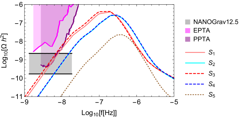
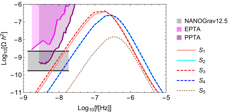
From Fig. 1 and Fig. 2, we show that the power spectra of GWs from the quark confinement phase transitions enter the 95% confidence interval from the NANOGrav 12.5-yr observation [1, 8], which indicates that the confinement/deconfinement phase transition in pure quark systems (cases of heavy static quarks with a zero baryon chemical potential and quarks with a finite baryon chemical potential) could possibly be the potential cosmological sources of the NANOGrav signal for both the Jouguet detonation and non-runaway bubble cases. The power spectra of GWs calculated from different holographic models (hard wall and soft wall) in a specific QCD matter system are different, but the difference does not change the conclusion. In contrast, the confinement/deconfinement transition in the pure gluon system could not possibly be the source of the NANOGrav signal. Since the critical phase transition temperatures for the cases of a finite chemical potential and a zero chemical potential are very close, the chemical potential has little effect on the power spectrum of GWs, and the quark confinement dominates the cosmological QCD transition according to the current NANOGrav observation. But these conclusions need to be further supported by more accurate observations of GWs in the future. We also calculate the spectrum indices from different holographic models, and find that the values are similar in the same bubble model. The values are about 2.78 and 2.91 for the Jouguet and non-runaway cases, respectively. These values could be used to check our conclusions with more accurate future observations.

4 Conclusions and Discussions

In this paper, we have showed that a possible stochastic common-spectrum process reported by the NANOGrav Collaboration based on the 12.5-yr PTA data can be explained potentially as a GW signal from the first-order cosmological confinement/deconfinement phase transition in the cases of (i) heavy static quarks with a zero baryon chemical potential and (ii) quarks with a finite baryon chemical potential. We also find that the gluon confinement could not possibly be the potential source of the NANOGrav signal based on the current observation. We match the GW spectra from the first-order phase transition in five different holographic QCD models with the NANOGrav signal. By considering both the Jouguet detonation and non-runaway bubble growth models, we find that the GW spectra from the confinement/deconfinement phase transition in pure quark systems, irrespective of whether the baryon chemical potential is finite or zero, enter the 95% confidence interval from the NANOGrav 12.5-yr observation [1, 8]. The baryon chemical potential has little influence on the power spectra of GWs produced by confinement/deconfinement phase transitions since the phase transition temperatures in both the finite baryon chemical potential case and zero chemical potential case are very close.

We must point out that we have assumed in our analysis that GWs are generated soon after the phase transition happens, so the temperature at which the GWs are produced is approximately the transition temperature. Although this is an acceptable assumption, it remains interesting to find a more credible holographic method to calculate the temperature $T_{\ast}$, analogous to what was done in Ref. [79]. Moreover, it is also worth considering the confinement/deconfinement phase transitions in possible QCD matter systems other than those we have looked at in the present paper and chiral symmetry breaking phase transitions. We would like to leave these to future studies.

References

- [1] Z. Arzoumanian et al. [NANOGrav Collaboration], Astrophys. J. Lett. 905, no. 2, L34 (2020).
- [2] G. Desvignes et al., Mon. Not. Roy. Astron. Soc. 458, no. 3, 3341 (2016).
- [3] M. Kerr et al., Publ. Astron. Soc. Austral. 37, e020 (2020).
- [4] B. B. P. Perera et al., Mon. Not. Roy. Astron. Soc. 490, no. 4, 4666 (2019).
- [5] J. Ellis and M. Lewicki, Phys. Rev. Lett. 126, no. 4, 041304 (2021).
- [6] S. Blasi, V. Brdar and K. Schmitz, Phys. Rev. Lett. 126, no. 4, 041305 (2021).
- [7] V. Vaskonen and H. Veermae, Phys. Rev. Lett. 126, no. 5, 051303 (2021).
- [8] V. De Luca, G. Franciolini and A. Riotto, Phys. Rev. Lett. 126, no. 4, 041303 (2021).
- [9] W. Buchmuller, V. Domcke and K. Schmitz, Phys. Lett. B 811, 135914 (2020).
- [10] Y. Nakai, M. Suzuki, F. Takahashi and M. Yamada, Phys. Lett. B 816, 136238 (2021).
- [11] A. Addazi, Y. F. Cai, Q. Gan, A. Marciano and K. Zeng, arXiv:2009.10327 [hep-ph].
- [12] W. Ratzinger and P. Schwaller, SciPost Phys. 10, 047 (2021).
- [13] K. Kohri and T. Terada, Phys. Lett. B 813, 136040 (2021).
- [14] R. Samanta and S. Datta, arXiv:2009.13452 [hep-ph].
- [15] S. Vagnozzi, Mon. Not. Roy. Astron. Soc. 502, no. 1, L11 (2021).
- [16] L. Bian, R. G. Cai, J. Liu, X. Y. Yang and R. Zhou, Phys. Rev. D 103, no. 8, L081301 (2021).
- [17] A. Neronov, A. Roper Pol, C. Caprini and D. Semikoz, Phys. Rev. D 103, L041302 (2021).
- [18] H. H. Li, G. Ye and Y. S. Piao, Phys. Lett. B 816, 136211 (2021).
- [19] A. Paul, U. Mukhopadhyay and D. Majumdar, arXiv:2010.03439 [hep-ph].
- [20] G. Domenech and S. Pi, arXiv:2010.03976 [astro-ph.CO].
- [21] S. Bhattacharya, S. Mohanty and P. Parashari, Phys. Rev. D 103, no. 6, 063532 (2021).
- [22] K. T. Abe, Y. Tada and I. Ueda, arXiv:2010.06193 [astro-ph.CO].
- [23] K. Inomata, M. Kawasaki, K. Mukaida and T. T. Yanagida, Phys. Rev. Lett. 126, no. 13, 131301 (2021).
- [24] H. Middleton, A. Sesana, S. Chen, A. Vecchio, W. Del Pozzo and P. A. Rosado, Mon. Not. Roy. Astron. Soc. 502, no. 1, L99 (2021).
- [25] S. Kuroyanagi, T. Takahashi and S. Yokoyama, JCAP 2101, 071 (2021).
- [26] A. K. Pandey, Eur. Phys. J. C 81, no. 5, 399 (2021).
- [27] N. Ramberg and L. Visinelli, Phys. Rev. D 103, no. 6, 063031 (2021).
- [28] B. Barman, A. Dutta Banik and A. Paul, arXiv:2012.11969 [astro-ph.CO].
- [29] V. Atal, A. Sanglas and N. Triantafyllou, arXiv:2012.14721 [astro-ph.CO].
- [30] Z. C. Chen, C. Yuan and Q. G. Huang, arXiv:2101.06869 [astro-ph.CO].
- [31] F. Bigazzi, A. Caddeo, A. L. Cotrone and A. Paredes, JHEP 2104, 094 (2021).
- [32] S. Datta, A. Ghosal and R. Samanta, arXiv:2012.14981 [hep-ph].
- [33] Y. Aoki, Z. Fodor, S. D. Katz and K. K. Szabo, Phys. Lett. B 643, 46 (2006).
- [34] A. Bazavov et al., Phys. Rev. D 85, 054503 (2012).
- [35] T. Bhattacharya et al., Phys. Rev. Lett. 113, no. 8, 082001 (2014).
- [36] A. Kosowsky, M. S. Turner and R. Watkins, Phys. Rev. D 45 (1992) 4514.
- [37] A. Kosowsky, M. S. Turner and R. Watkins, Phys. Rev. Lett. 69, 2026 (1992).
- [38] A. Kosowsky and M. S. Turner, Phys. Rev. D 47, 4372 (1993).
- [39] M. Kamionkowski, A. Kosowsky and M. S. Turner, Phys. Rev. D 49, 2837 (1994).
- [40] C. Caprini, R. Durrer and G. Servant, Phys. Rev. D 77, 124015 (2008).
- [41] S. J. Huber and T. Konstandin, JCAP 0809, 022 (2008).
- [42] C. Caprini et al., JCAP 1604, 001 (2016).
- [43] M. Hindmarsh, S. J. Huber, K. Rummukainen and D. J. Weir, Phys. Rev. Lett. 112, 041301 (2014).
- [44] J. T. Giblin, Jr. and J. B. Mertens, JHEP 1312, 042 (2013).
- [45] J. T. Giblin and J. B. Mertens, Phys. Rev. D 90, no. 2, 023532 (2014).
- [46] M. Hindmarsh, S. J. Huber, K. Rummukainen and D. J. Weir, Phys. Rev. D 92, no. 12, 123009 (2015).
- [47] A. Kosowsky, A. Mack and T. Kahniashvili, Phys. Rev. D 66, 024030 (2002).
- [48] C. Caprini and R. Durrer, Phys. Rev. D 74, 063521 (2006).
- [49] T. Kahniashvili, A. Kosowsky, G. Gogoberidze and Y. Maravin, Phys. Rev. D 78, 043003 (2008).
- [50] T. Kahniashvili, L. Campanelli, G. Gogoberidze, Y. Maravin and B. Ratra, Phys. Rev. D 78, 123006 (2008) Erratum: [Phys. Rev. D 79, 109901 (2009)].
- [51] T. Kahniashvili, L. Kisslinger and T. Stevens, Phys. Rev. D 81, 023004 (2010).
- [52] C. Caprini, R. Durrer and G. Servant, JCAP 0912, 024 (2009).
- [53] L. Kisslinger and T. Kahniashvili, Phys. Rev. D 92, no. 4, 043006 (2015).
- [54] C. Caprini, R. Durrer and X. Siemens, Phys. Rev. D 82, 063511 (2010).
- [55] S. Anand, U. K. Dey and S. Mohanty, JCAP 1703, 018 (2017).
- [56] M. Ahmadvand and K. Bitaghsir Fadafan, Phys. Lett. B 772, 747 (2017).
- [57] O. Philipsen, arXiv:1009.4089 [hep-lat].
- [58] P. Petreczky, J. Phys. G 39, 093002 (2012).
- [59] D. J. Schwarz and M. Stuke, JCAP 0911, 025 (2009) Erratum: [JCAP 1010, E01 (2010)].
- [60] M. Ahmadvand and K. Bitaghsir Fadafan, Phys. Lett. B 779, 1 (2018).
- [61] Y. Chen, M. Huang and Q. S. Yan, JHEP 1805, 178 (2018).
- [62] P. J. Steinhardt, Phys. Rev. D 25, 2074 (1982).
- [63] A. Nicolis, Class. Quant. Grav. 21, L27 (2004).
- [64] J. R. Espinosa, T. Konstandin, J. M. No and G. Servant, JCAP 1006, 028 (2010).
- [65] J. M. Maldacena, Int. J. Theor. Phys. 38, 1113 (1999) [Adv. Theor. Math. Phys. 2, 231 (1998)].
- [66] S. S. Gubser, I. R. Klebanov and A. M. Polyakov, Phys. Lett. B 428, 105 (1998).
- [67] E. Witten, Adv. Theor. Math. Phys. 2, 253 (1998).
- [68] J. Erlich, E. Katz, D. T. Son and M. A. Stephanov, Phys. Rev. Lett. 95, 261602 (2005).
- [69] S. W. Hawking and D. N. Page, Commun. Math. Phys. 87, 577 (1983).
- [70] C. P. Herzog, Phys. Rev. Lett. 98, 091601 (2007).
- [71] N. Horigome and Y. Tanii, JHEP 0701, 072 (2007).
- [72] Y. Kim, B. H. Lee, S. Nam, C. Park and S. J. Sin, Phys. Rev. D 76, 086003 (2007).
- [73] Y. Seo, J. P. Shock, S. J. Sin and D. Zoakos, JHEP 1003, 115 (2010).
- [74] R. G. Cai, S. He and D. Li, JHEP 1203, 033 (2012).
- [75] S. Takeda, Y. Kuramashi and A. Ukawa, Phys. Rev. D 85, 096008 (2012).
- [76] M. Fromm, J. Langelage, S. Lottini and O. Philipsen, JHEP 1201, 042 (2012).
- [77] H. T. Ding, PoS LATTICE 2016, 022 (2017).
- [78] M. Ahmadvand, K. Bitaghsir Fadafan and S. Rezapour, arXiv:2006.04265 [hep-th].
- [79] L. Randall and G. Servant, JHEP 0705, 054 (2007).