TCLR: Temporal Contrastive Learning for Video Representation

Abstract

Contrastive learning has nearly closed the gap between supervised and self-supervised learning of image representations, and has also been explored for videos. However, prior work on contrastive learning for video data has not explored the effect of explicitly encouraging the features to be distinct across the temporal dimension. We develop a new temporal contrastive learning framework consisting of two novel losses to improve upon existing contrastive self-supervised video representation learning methods. The local-local temporal contrastive loss adds the task of discriminating between non-overlapping clips from the same video, whereas the global-local temporal contrastive aims to discriminate between timesteps of the feature map of an input clip in order to increase the temporal diversity of the learned features. Our proposed temporal contrastive learning framework achieves significant improvement over the state-of-the-art results in various downstream video understanding tasks such as action recognition, limited-label action classification, and nearest-neighbor video retrieval on multiple video datasets and backbones. We also demonstrate significant improvement in fine-grained action classification for visually similar classes. With the commonly used 3D ResNet-18 architecture with UCF101 pretraining, we achieve 82.4% (+5.1% increase over the previous best) top-1 accuracy on UCF101 and 52.9% (+5.4% increase) on HMDB51 action classification, and 56.2% (+11.7% increase) Top-1 Recall on UCF101 nearest neighbor video retrieval. Code released at https://github.com/DAVEISHAN/TCLR.

1 Introduction

Large-scale labeled datasets such as Kinetics [10], LSHVU [17] etc have been crucial for recent advances in video understanding tasks. Since training a video encoder using existing supervised learning approaches is label-inefficient [32], annotated video data is required at a large scale. This costs enormous human effort and time, much more so than annotating images. At the same time, a tremendous amount of unlabeled video data is easily available on the internet. Research in self-supervised video representation learning can unlock the corpus of readily available unlabeled video data and unshackle progress in video understanding.

Recently, Contrastive Self-supervised Learning (CSL) based methods [12, 27, 9] have demonstrated the ability to learn powerful image representations in a self-supervised manner, and have narrowed down the performance gap between unsupervised and supervised representation learning on various image understanding downstream tasks.

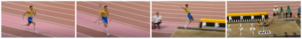
(a)

(b)

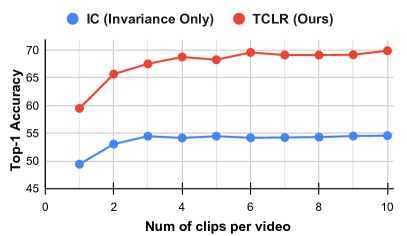
(c)

Figure 1: Videos from standard action recognition datasets often have distinct temporal stages. For example, in figure (a) we can see the two distinct stages (Running and Jumping) of the LongJump action. Typically predictions across multiple short clips are aggregated, as a single short clip may not capture both stages of the action. We show the comparison of vanilla instance discrimination based contrastive (IC) self-supervision and our proposed TCLR method on (b) Nearest neighbour retrieval and (c) Linear classification tasks. We find that IC trained models do not benefit much from using multiple clips during evaluation. This is a result of IC imposing within instance temporal invariance. This motivates our proposed TCLR pre-training, which explicitly encourages learning distinct features across time.

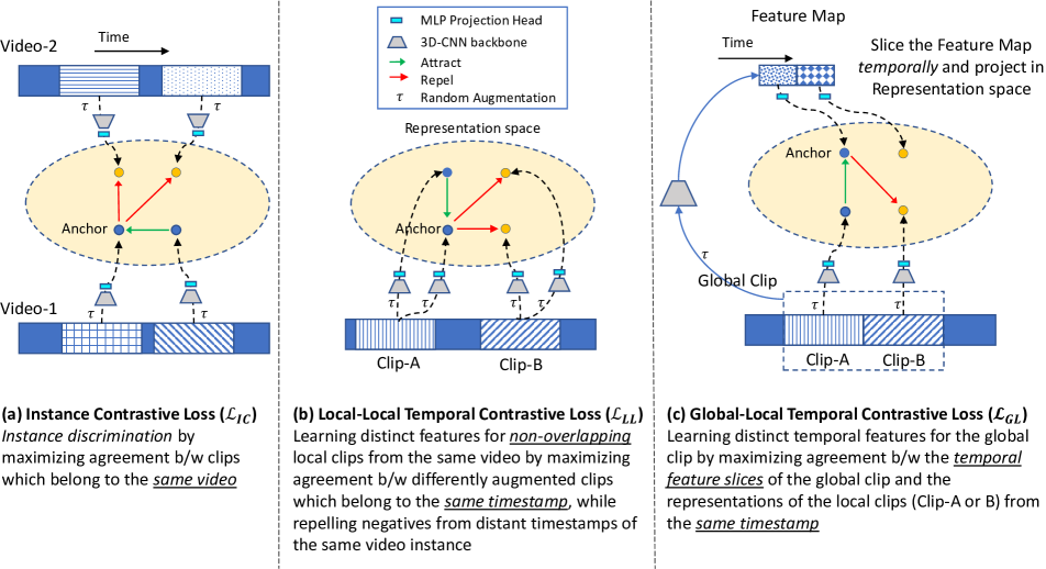
Figure 2: The proposed temporal contrastive learning framework (TCLR) for learning temporally distinct video representations consists of three different losses.

A simple yet effective extension of CSL to the video domain can be obtained by using the InfoNCE instance discrimination objective, where the model learns to distinguish clips of a given video from the clips of other videos in the dataset (see Figure 2a). Unlike images, videos have both time-invariant and the temporally varying properties. For example, in a LongJump video from UCF101 (See Figure 1), running and jumping represent two very different stages of the action. Usually, video understanding models utilize temporally varying features by aggregating along the temporal dimension to obtain a video level prediction. While the significant success can be achieved on many video understanding tasks by only modelling the temporally invariant properties, it maybe possible that the temporally varying properties can also play an important role in further improvements on these tasks. Whether video representations should be invariant or distinct along the temporal dimension is an open question in the literature. Instance contrastive pre-training, however, encourages the model to learn similar features to represent temporally distant clips from the video, i.e. it enforces temporal invariance on the features. While instance level contrastive learning lies on one end of the spectrum, some recent works have tried to relax the invariance constraint through various means, such as, using a weighted temporal sampling strategy to avoid enforcing invariance between temporally distant clips [49], cross-modal mining of positive samples from across video instances [25] or adding additional pretext tasks that require learning temporal features [63, 50, 69, 5].

We take a different approach by explicitly encouraging the learning of temporally distinct video representations. The challenge with video classification is modelling variable length videos with a fixed number of parameters. 3D CNNs tackle this challenge by temporal aggregation of features across two levels: averaging across distinct fixed length temporal segments of a video (clips) and also temporal pooling across the feature map of each clip. Based on this observation, we propose two different temporal contrastive losses in order to learn temporally distinct features across the video: one which acts across clips of the same video, and another which acts across the timesteps of the feature map of the same clip. Combined with the vanilla instance contrastive loss, these novel losses result in an increase in the temporal diversity of the learned features, and better accuracy on downstream tasks.

Our first proposed loss is the local-local temporal contrastive loss (Figure 2b), which ensures that temporally non-overlapping clips from the same video are mapped to distinct representations. This loss treats randomly augmented versions of the same clip as positive pairs to be brought together, and other non-overlapping clips from the same video as negative matches to be pushed away. While the local-local loss ensures that distinct clips have distinct representations, in order to encourage temporal variation within each clip, we introduce a second temporal contrastive loss, the global-local temporal contrastive loss (Figure 2c). This loss constrains the timesteps of the feature map of a long “global” video clip to match the representations of the temporally aligned shorter “local” video clips.

Our complete framework is called Temporal Contrastive Learning of video Representations (henceforth referred to as TCLR). TCLR retains the ability of representations to successfully discriminate between video instances due to its instance contrastive loss. In addition, TCLR attempts to capture the within-instance temporal variation. Through extensive experiments on various downstream video understanding tasks, we demonstrate that both of our proposed Temporal Contrastive losses contribute to the learning of powerful video representations, and provide significant improvements.

The original contributions of this work can be summarized as below:

• TCLR is the first contrastive learning framework to explicitly enforce within instance temporal feature variation for video understanding tasks.

• Novel local-local and global-local temporal contrastive losses, which when combined with the standard instance contrastive loss significantly outperform the state-of-the-art on various downstream video understanding tasks like action recognition, nearest neighbor video retrieval and action classification with limited labeled data, while using 3 different 3D CNN architectures and 2 datasets (UCF101 & HMDB51).

• We propose the use of the challenging Diving48 fine-grained action classification task for evaluating the quality of learned video representations.

2 Related Work

Recent approaches for self-supervised video representation learning can be categorized into two major groups based on the self-supervised learning objective: (1) Pretext task based methods, and (2) Contrastive Learning based methods.

Pretext task based approaches: Various pretext tasks have been devised for self-supervised video representation learning based on learning the correct temporal order of the data: verifying correct frame order [44], identifying the correctly ordered tuple from a set of shuffled orderings [20, 53], sorting frame order [37], and predicting clip order [66]. Some methods extend existing pretext tasks from the image domain to video domain, for example, solving spatio-temporal jigsaw puzzles [2, 33, 28] and identifying the rotation of transformed video clips [31]. Many recent works rely on predicting video properties like playback rate of the video [13, 70, 63, 50], temporal transformation that has been applied from a given set [30, 29], speediness of moving objects [7], and motion and appearance statistics of the video [62, 61].

Contrastive Self-supervised Learning (CSL) based approaches: Following the success of contrastive learning approaches of self-supervised image representation learning such as SimCLR [12] and MoCo [27], there have been many extensions of contrastive learning to the video domain. For instance, various video CSL methods [63, 46, 5, 49, 54, 69, 56, 50, 68] leverage Instance level Discrimination objectives, and build their method upon them, where clips from the same video are treated as positives and clips from the different videos as negatives. CVRL [49] studies the importance of temporal augmentation and develops a temporal sampler to avoid enforcing excessive temporal invariance in learning video representation. VideoMoCo [46] improves image-based MoCo framework for video representation by encouraging temporal robustness of the encoder and modeling temporal decay of the keys. VTHCL [68] employs SlowFast architecture [18] and uses contrastive loss with the slow and fast pathway representations as the positive pair. VIE [72] is proposed as a deep neural embedding-based method to learn video representation in an unsupervised manner, by combining both static image representation from 2D CNN and dynamic motion representation from 3D CNN. Generative contrastive learning-based approaches such as predicting the the dense representation of the next video block [23, 24], or Contrastive Predictive Coding (CPC) [45] for videos [40] have also been studied in the literature.

AMDIM [4] is another CSL approach for image representation learning, where a local view (spatial slice of the feature map taken from an intermediate layer) and a global view (full feature map) of differently augmented versions of the same image are considered as a positive pair, and global views of other images form negative pair of the contrastive loss. The method is adapted for the video domain [16, 67] by generating local views from the spatio-temporal features. Unlike this class of methods, which try to maximize agreement across features from different levels of the encoder, our Global-Local loss tries to learn distinct features across temporal slices of the feature map instead.

Some recent works combine pretext tasks along with contrastive learning in a multi-task setting to learn temporally varying features in the video representation. For example, using video clips with different playback rates as positive pairs for contrastive loss along with predicting the playback rate [63], or temporal transforms [5]. Other works propose frame-based contrastive learning, along with existing pretext tasks of frame rotation prediction [35] and frame-tuple order verification [69]. Unlike these works, TCLR takes a different approach by adding explicit temporal contrastive losses that encourage temporal diversity in the learned features, instead of utilizing a pretext task for this purpose.

Some works which try to capture intra-video variance using optical flow, but are nevertheless interesting to compare with. IIC [54] uses intra-instance negatives, but it relies on frame repeating and shuffling to generate these “hard” negatives, and does not focus on learning distinct features across the temporal axis. DSM [60] tries to decouple scene and motion features by an intra-instance triplet loss, which uses negatives generated by optical flow scaling and spatial warping. Some recent works use extra supervisory signals in addition to the RGB video data to learn video representation in a self-supervised manner. However, these methods either require additional cross-modal data (e.g. text narration [42], audio [1]) or expensive and time-consuming computation of hand-crafted visual priors (e.g. optical flow [54, 52, 64, 55, 25] or dense trajectories [56]). In this work we focus only on learning from RGB data without using any auxiliary data from any extra modality or additionally computed visual priors.

3 Method

The key idea in our proposed framework is to learn two levels of contrastive discrimination: instance discrimination using the instance contrastive loss and within-instance temporal level discrimination using our novel temporal contrastive losses. The two different temporal contrastive losses which are applied within the same video instance: Local-Local Loss and Global-Local loss. Each of these losses is explained in the following sections.

3.1 Instance Contrastive Loss

We leverage the idea of instance discrimination using InfoNCE [22] based contrastive loss for learning video representations. In the video domain, in addition to leveraging image-based spatial augmentations, temporal augmentations can also be applied to generate different transformed versions of a particular instance. For a video instance, we extract various clips (starting from different timestamps and/or having different frame sampling rates). We consider a randomly sampled mini-batch of size $N_{B}$ from different video instances, and from each instance we extract a pair of clips from random timesteps resulting in a total of 2N clips. The extracted clips are augmented using standard stochastic appearance and geometric transformations. Each of the transformed clips is then passed through a 3D-CNN based video encoder which is followed by a non-linear projection head (multi-layer perceptron) to project the encoded features on the representation space. Hence, for each video-instance $i$ we get two clip representations $(G_{i},G^{\prime}_{i})$. The instance contrastive loss is defined as follows:

$$\small\mathcal{L}_{IC}^{i}=-\log\frac{h\left(G_{i},G^{\prime}_{i}\right)}{\sum_{j=1}^{N_{B}}[\mathbb{1}_{[j\neq i]}h(G_{i},G_{j})+h(G_{i},G^{\prime}_{j})]},$$ (1)

where, $h(u,v)=\exp\left(u^{T}v/(\|u\|\|v\|\theta)\right)$ is used to compute the similarity between $u$ and $v$ vectors with an adjustable parameter temperature, $\theta$. $\mathbb{1}_{[j\neq i]}\in\{0,1\}$ is an indicator function which equals 1 iff $j\neq i$.

3.2 Temporal Contrastive Losses

For self-supervised training using the instance contrastive loss of Equation 1, the model is presented with multiple clips cropped from random spatio-temporal locations within a single video as positive matches. This encourages the model to become invariant to the inherent variation present within an instance. In order to enable contrastive learning to represent within instance temporal variation, we introduce two novel temporal contrastive losses: local-local temporal contrastive loss and global-local temporal contrastive loss.

3.2.1 Local-Local Temporal Contrastive Loss

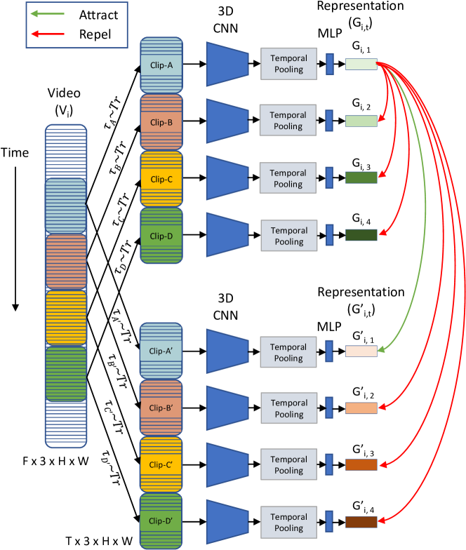
Figure 3: Local-Local Temporal Contrastive Loss is applied to representations of non-overlapping clips extracted from same video instance $i$. For the clip starting at timestep $p$, two randomly transformed versions are generated and their representations $G_{i,p}$ and $G^{\prime}_{i,p}$ serve as the positive pair for the loss, whereas the other non-overlapping clips along with the anchor, $G_{i,p}$, form the negative pairs. $p=1$ serves as anchor, further details in Section 3.2.1. $\tau_{A}$, $\tau_{A^{\prime}}$, …, $\tau_{D^{\prime}}$ are random set of augmentation sampled from universal set $Tr$.

For this loss, we treat non-overlapping clips sampled from different temporal segments of the same video instance as negative pairs, and randomly transformed versions of the same clip as a positive pair.

The local-local loss is defined by Equation 2 and illustrated in Figure 3. A given video instance $i$ is divided into $N_{clips}$ non-overlapping clips. For the anchor clip starting at timestep $p$, its representation $G_{i,p}$, and the representation of its transformed version form the positive pair ($G_{i,p}$,$G^{\prime}_{i,p})$ for this loss; whereas the other $N_{clips}-1$ clips from the same video instance (and their transformed versions) form the negative pairs. Hence, for every positive pair, the local-local contrastive loss has $2\times N_{clips}-2$ negative pairs as defined in the following loss:

$$\small\mathcal{L}_{LL}^{i}=-\sum_{p=1}^{N_{clips}}\log\frac{h\left(G_{i,p},G^{\prime}_{i,p}\right)}{\sum_{q=1}^{N_{clips}}[\mathbb{1}_{[q\neq p]}h(G_{i,p},G_{i,q})+h(G_{i,p},G^{\prime}_{i,q})]}.$$ (2)

The key difference between the Instance contrastive loss (Equation 1) and the proposed Local-Local Temporal contrastive loss (Equation 2) is that for the local-local loss the negatives come from the same video instance but from a different temporal segment (clips), whereas in Equation 1, the negative pairs come from different video instances.

3.2.2 Global-Local Temporal Contrastive Loss

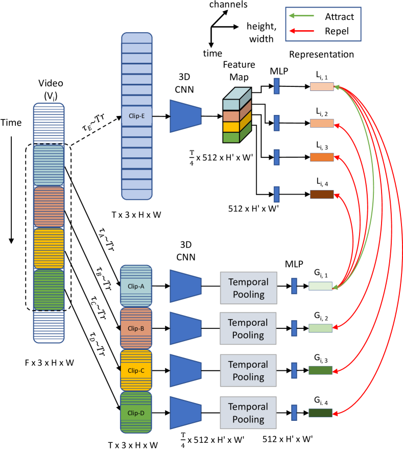
Figure 4: Global-Local Temporal Contrastive Loss A global clip (Clip E) is extracted from a video instance and divided into 4 equal length local clips (Clips A through D). The global clip is temporally downsampled to have the same number of frames as each local clip. The local representations $L_{i,1}$ through $L_{i,4}$ from the global clip are obtained from the penultimate layer of the 3D-CNN (prior to temporal pooling). Global representations of the local clips, $G_{i,1}$ through $G_{i,4}$ are obtained from the CNN (after temporal pooling layer). This loss aims to maximize the similarity between the local representation of the global clip and the global representations of the corresponding local clip. Further details in Section 3.2.2.

The feature map in the higher layers of 3D CNNs are capable of representing temporal variation in the input clip, which is temporally pooled before being used for classification, or projected in the representation space in the case of contrastive learning. The objective of our proposed global-local temporal contrastive loss is to explicitly encourage the model to learn feature maps that represent the temporal locality of the input clip across temporal dimension of the feature map.

This loss is illustrated in Figure 4. The notion of local and global is used at two different levels: at the input clip level and the feature level. Clip-E is a global clip and Clip A-D are local clips contained within Clip-A. Features are referred to as global after the final pooling operation and a temporal slice of the feature map before the pooling operation is referred to as a local feature. In Figure 4, $L_{i,1}$ is the local feature of the global Clip-A and $G_{i,1}$ is the global feature of the local Clip-B.

For a video instance $i$, divided into $N_{clips}$ clips, the local clip $k$ can either be represented by a global (pooled) representation $G_{i,k}$ or a local representation $L_{i,k}$ of the corresponding timestep in the feature map of the global clip. This loss has two sets of reciprocal terms, with $G_{i,k}$ and $L_{i,k}$ serving as the anchor for each term. The negative pairs are supplied by matching the anchors with representations corresponding to other non-overlapping local clips. Note that similar to our local-local temporal contrastive loss we do not use negatives from other video instances for calculating this loss. The loss is defined by the following equations:

$$\small\mathcal{L}_{GL_{k}}^{i}=\log\frac{h\left(L_{i,k},G_{i,k}\right)}{\sum_{q=1}^{N_{clips}}h(L_{i,k},G_{i,q})}+\log\frac{h\left(G_{i,k},L_{i,k}\right)}{\sum_{q=1}^{N_{clips}}h(G_{i,k},L_{i,q})},$$ (3)

$$\small\mathcal{L}_{GL}^{i}=-\sum_{k=1}^{N_{clips}}\mathcal{L}_{GL_{k}}^{i}.$$ (4)

4 Experiments

Datasets and Implementation: We use three action recognition datasets: UCF101 [51], Kinetics400 [10], and HMDB51 [36] for our experiments. We use the three most commonly used networks from the literature: 3D-ResNet-18 (R3D-18) [26], R(2+1)D-18 [58], and C3D [57] for our experiments. For non-linear projection head, we use a multi-layer perceptron with 1-hidden layer following experimental setting of [12]. We utilize 4 local clips per global clip for the global-local temporal contrastive loss. For all reported results, we utilize commonly used random augmentations including appearance-based transforms such as grayscale, channel dropping, and color jittering and geometry-based transforms like random scaling, random cropping, random cut-out and random horizontal-flip. Our results can be further improved by using more complex augmentations like Gaussian blurring, shearing and rotation, however these are not used in the results reported in this paper. We provide results with more complex augmentation in Section D of the supplementary material. For self-supervised pretraining we use UCF101 training set (split-1) or Kinetics400 training set, without using any class labels. For all self-supervised pretraining, supervised finetuning and other downstream tasks, we use clips of 16 frames with a resolution of $112\times 112$. More implementation details can be found in Section C of the supplementary material.

4.1 Evaluating Self-supervised Representations

We evaluate the learned video representation using different downstream video understanding tasks: i) action recognition and ii) nearest neighbor video retrieval on UCF101 and HMDB51 datasets, and iii) limited label training on UCF101, following protocols from prior works [24]. We also evaluate our learned representations on the challenging Diving-48 fine-grained action recognition task [39]; to the best of our knowledge TCLR is the first work that reports result on this challenging task. Our method is also employed in Knights [15] to get first place in ICCV-21 Action recognition challenge [38].

Action Recognition on UCF101 and HMDB51:

Method	Venue	Input Size	UCF101 Pre-Training		Kinetics400 Pre-Training
			UCF101	HMDB51	UCF101	HMDB51
Backbone: R3D-18
ST-Puzzle [33]	AAAI-19	$16\times 112$	$-$	$-$	$65.8$	$33.7$
STS [61]	TPAMI-21	$16\times 112$	$67.2$	$32.7$	$68.1$	$34.4$
DPC [23]	ICCVw-19	$40\times 128$	$60.6$	$-$	$68.2$	$34.5$
VCOP [66]	CVPR-20	$16\times 112$	$64.9$	$29.5$	$-$	$-$
Pace Pred [63]	ECCV-20	$16\times 112$	$65.0$	$-$	$-$	$-$
VCP [41]	AAAI-20	$16\times 112$	$66.0$	$31.5$	$-$	$-$
PRP [70]	CVPR-20	$16\times 112$	$66.5$	$29.7$	$-$	$-$
Var. PSP [13]	Access-21	$16\times 112$	$69.0$	$33.7$	$-$	$-$
MemDPC [24]	ECCV-20	$40\times 224$	$69.2$	$-$	$-$	$-$
TCP [40]	WACV-21	$-\times 224$	$64.8$	$34.7$	$70.5$	$41.1$
VIE [72]	CVPR-20	$16\times 112$	$-$	$-$	$72.3$	$44.8$
UnsupIDT [56]	ECCVw-20	$16\times 112$	$-$	$-$	$73.0$	$41.6$
CSJ [28]	-	$16\times 224$	$70.4$	$36.0$	$76.2$	$46.7$
BFP [6]	WACV-21	$40\times 128$	$63.6$	$-$	$66.4$	$45.3$
IIC (RGB) [54]	ACMMM-20	$16\times 112$	$61.6$	$-$	$-$	$-$
CVRL (Reproduced) [49]	CVPR-21	$16\times 112$	$75.77$	$44.6$	$-$	$-$
SSTL [50]	-	$16\times 112$	$-$	$-$	$79.1$	$49.7$
VTHCL [68]	-	$8\times 224$	$-$	$-$	$80.6$	$48.6$
VideoMoCo [46]	CVPR-21	$16\times 112$	$-$	$-$	$74.1$	$43.6$
RSPNet [11]	AAAI-21	$16\times 112$	$-$	$-$	$74.3$	$41.8$
Temp Trans [30]	ECCV-20	$16\times 112$	$77.3$	$47.5$	$79.3*$	$49.8*$
TaCo [5]	-	$16\times 224$	$-$	$-$	${\color[rgb]{0,0,1}81.4}$	$45.4$
MFO [48]	ICCV-21	$16\times 112$	$-$	$-$	$79.1$	$47.6$
TCLR		$16\times 112$	$82.4$	$52.9$	$84.1$	$53.6$
TCLR (Best Ablation)		$16\times 112$	$83.9$	$53.5$	$85.4$	$55.4$
Backbone: R(2+1)D-18
VCP [41]	AAAI-20	$16\times 112$	$66.3$	$32.2$	$-$	$-$
PRP [70]	CVPR-20	$16\times 112$	$72.1$	$35.0$	$-$	$-$
VCOP [66]	CVPR-20	$16\times 112$	$72.4$	$30.9$	$-$	$-$
Pace Pred [63]	ECCV-20	$16\times 112$	$75.9$	$35.9$	$77.1$	$36.6$
STS [61]	TPAMI-21	$16\times 112$	$73.6$	$34.1$	$77.8$	$40.5$
VideoMoCo [46]	CVPR-21	$16\times 112$	$-$	$-$	$78.7$	${\color[rgb]{0,0,1}49.2}$
VideoDIM [16]	-	$32\times 128$	$-$	$-$	$79.7*$	$49.2*$
RSPNet [11]	AAAI-21	$16\times 112$	$-$	$-$	$81.1$	$44.6$
Temp Trans [30]	ECCV-20	$16\times 112$	$81.6$	$46.4$	$-$	$-$
TaCo [5]	-	$16\times 224$	$-$	$-$	${\color[rgb]{0,0,1}81.8}$	$46.0$
TCLR		$16\times 112$	$82.8$	$53.6$	$88.2$	$60.0$
Backbone: C3D
MA Stats-1 [62]	CVPR-19	$16\times 112$	$58.8$	$32.6$	$61.2$	$33.4$
Temp Trans [30]	ECCV-20	$16\times 112$	$68.3$	$38.4$	$69.9*$	$39.6*$
PRP [70]	CVPR-20	$16\times 112$	$69.1$	$34.5$	$-$	$-$
VCP [41]	AAAI-20	$16\times 112$	$68.5$	$32.5$	$-$	$-$
VCOP [66]	CVPR-20	$16\times 112$	$65.6$	$28.4$	$-$	$-$
Pace Pred [63]	ECCV-20	$16\times 112$	$68.0$	$-$	$-$	$-$
STS [61]	TPAMI-21	$16\times 112$	$69.3$	$34.2$	$71.8$	$37.8$
Var. PSP [13]	Access-21	$16\times 112$	$70.4$	$34.3$	$-$	$-$
DSM [60]	AAAI-21	$16\times 112$	$70.3$	${\color[rgb]{0,0,1}40.5}$	$-$	$-$
TCLR		$16\times 112$	$76.1$	$48.6$	$-$	$-$
Other Configurations
CVRL (R3D-50) [49]	CVPR-21	$32\times 224$	$-$	$-$	$92.2$	$66.7$
RSPNet (S3D-G) [11]	AAAI-21	$64\times 224$	$-$	$-$	$93.7$	$64.7$
CoCLR† (S3D-23) [25]	NeurIPS-20	$16\times 112$	$87.3$	$58.7$	$90.6$	$62.9$
SpeedNet (S3D-G) [7]	CVPR-20	$16\times 224$	$-$	$-$	$81.1$	$48.8$
$\rho$SimCLR (R50) [19]	CVPR-21	$8\times 224$	$-$	$-$	$85.6$	$-$
SeCO (R50+TSN) [69]	AAAI-21	$50\times 224$	$-$	$-$	$88.3\ddagger$	$55.6\ddagger$

Table 1: Finetuning Results (average of 3 splits) for action classification on UCF101 and HMDB51. Self supervised pretraining was done on UCF101 (left) and Kinetics (right). ^† indicates models that utilize optical flow. $*$ indicates Kinetics-600 self-supervised pretraining. $\ddagger$ indicates ImageNet+Kinetics pre-training. Best and second best results are highlighted.

Method	Venue	UCF101				HMDB51
	R@1	R@5	R@10	R@20	R@1	R@5	R@10	R@20
Backbone: R3D-18
VCOP [66]	CVPR-20	$14.1$	$30.3$	$40.4$	$51.1$	$~{}7.6$	$22.9$	$34.4$	$48.8$
VCP [41]	AAAI-20	$18.6$	$33.6$	$42.5$	$53.5$	$~{}7.6$	$24.4$	$36.6$	$53.6$
Pace Pred [63]	ECCV-20	$23.8$	$38.1$	$46.4$	$56.6$	$~{}9.6$	$26.9$	$41.1$	$56.1$
Var. PSP [13]	Access-21	$24.6$	$41.9$	$51.3$	$62.7$	$10.3$	$26.6$	$38.8$	$51.6$
Temp Trans [30]	ECCV-20	$26.1$	$48.5$	$59.1$	$69.6$	$-$	$-$	$-$	$-$
STS* [61]	TPAMI-21	$38.3$	${\color[rgb]{0,0,1}59.9}$	$68.9$	$77.2$	$18.0$	$37.2$	$50.7$	${\color[rgb]{0,0,1}64.8}$
SSTL* [50]	-	$44.5$	$57.4$	$63.5$	$70.0$	$21.8$	$35.7$	$44.2$	$57.7$
CSJ* [28]	-	$21.5$	$40.5$	$53.2$	$64.9$	$-$	$-$	$-$	$-$
MemDPC [24]	ECCV-20	$20.2$	$40.4$	$52.4$	$64.7$	$~{}7.7$	$25.7$	$40.6$	$57.7$
RSPNet [11]	AAAI-21	$41.1$	$59.4$	$68.4$	$77.8$	$-$	$-$	$-$	$-$
MFO [48]	ICCV-21	$39.6$	$57.6$	${\color[rgb]{0,0,1}69.2}$	${\color[rgb]{0,0,1}78.0}$	$18.8$	${\color[rgb]{0,0,1}39.2}$	${\color[rgb]{0,0,1}51.0}$	$63.7$
TCLR	-	$56.2$	$72.2$	$79.0$	$85.3$	$22.8$	$45.4$	$57.8$	$73.1$
Backbone: C3D
VCOP [66]	CVPR-20	$12.5$	$29.0$	$39.0$	$50.6$	$5.7$	$19.5$	$30.7$	$45.8$
VCP [41]	AAAI-20	$17.3$	$31.5$	$42.0$	$52.6$	$7.8$	$23.8$	$35.3$	$49.3$
Pace Pred [63]	ECCV-20	$31.9$	$49.7$	$59.2$	$68.9$	$12.5$	$32.2$	$45.4$	$61.0$
DSM [63]	AAAI-21	$16.8$	$33.4$	$43.4$	$54.6$	$8.2$	$25.9$	$38.1$	$52.0$
STS* [61]	TPAMI-21	${\color[rgb]{0,0,1}39.1}$	${\color[rgb]{0,0,1}59.2}$	${\color[rgb]{0,0,1}68.8}$	${\color[rgb]{0,0,1}77.6}$	$16.4$	${\color[rgb]{0,0,1}36.9}$	${\color[rgb]{0,0,1}49.9}$	${\color[rgb]{0,0,1}64.9}$
RSPNet [11]	AAAI-21	$36.0$	$56.7$	$66.5$	$76.3$	$-$	$-$	$-$	$-$
TCLR	-	$48.6$	$67.6$	$75.5$	$82.5$	$19.3$	$43.3$	$57.6$	$70.1$
Backbone: R(2+1)D-18
VCOP [66]	CVPR-20	$10.7$	$25.9$	$35.4$	$47.3$	$7.4$	$22.6$	$34.4$	$48.5$
VCP [41]	AAAI-20	$19.9$	$33.7$	$42.0$	$50.5$	$6.7$	$21.3$	$32.7$	$49.2$
Pace Pred [63]	ECCV-20	$25.6$	$42.7$	$51.3$	$61.3$	$12.9$	$31.6$	$43.2$	$58.0$
STS* [61]	TPAMI-21	$38.1$	$58.9$	$68.1$	$77.0$	$16.4$	$36.9$	$50.5$	$65.4$
TCLR	-	$56.9$	$72.2$	$79.0$	$84.6$	$24.1$	$45.8$	$58.3$	$75.3$

Table 2: Nearest neighbor video retrieval results on UCF101 and HMDB51, after self-supervised pretraining on UCF101. ^*marks models pretrained on Kinetics-400. Best and second best results highlighted. Methods based on optical flow and audio modalities are excluded.

For the action recognition task on UCF101 and HMDB51, we first pretrain different video encoders in self-supervised manner on UCF101 or Kinetics400, and then perform supervised fine-tuning. In order to ensure fair comparison, we evaluate the method on the three most commonly used 3D CNN backbones in the prior works, while also listing details about the input clip resolution and number of frames used, as it is known to affect the results significantly [58, 47]. Comparison results are shown in Table 1. Previous results based on multi-modal approaches that utilize text, audio etc are excluded [47, 3, 43]. Results from prior works which do not utilize the three common architectures or use optical flow as input are presented in grey. We reproduce the results for CVRL [49] using the R3D-18 model and 112 resolution, and carefully implement their temporal sampling and augmentation strategy. TCLR consistently outperforms the state-of-art by wide margins for all comparable combinations of backbone, pre-training dataset and fine-tuning dataset. The best prior results are reported by TaCo [5], which relies on learning temporal features using pretext tasks on top of instance discrimination. Our consistent improvement over TaCo suggests that using temporal contrastive losses results in better features than using existing temporal pre-text tasks in a multi-task setting.

Nearest Neighbor Video Retrieval:

We evaluate the learned representation by performing nearest neighbor retrieval after self-supervised pretraining on UCF101 videos and without any supervised finetuning. Videos from the test set are used as the query and the training set as the search gallery, following the protocol used in prior work [24]. Results for retrieval are presented for both UCF101 and HMDB51 in Table 2. TCLR outperforms previous state-of-the-art in UCF101 Top-1 Retrieval by 12% to 30% depending on the architecture

Label Efficiency/ Finetuning with limited data: We evaluate our pretrained model for action recognition task on UCF101 (split-1) with limited labeled training data following the protocols from prior work [24, 31, 21]. Our method outperforms MotionFit [21], MemDPC [24] and RotNet3D [31] in all settings of limited percentage of training data as shown in Figure 5. This result in addition to NN results demonstrate that the learned representations from TCLR are significantly better than other recent works, TCLR can achieve competitive performance to MemDPC with only 10% of the labeled data.

Figure 5: Evaluating Label Efficiency using Limited Label Learning on UCF101 (split-1) action classification task.

Experiments on Diving-48 Dataset: This task presents some additional challenges over and above the standard action recognition task: action categories in Diving48 are defined by a combination of takeoff (dive groups), movements in flight (somersaults and/or twists), and entry (dive positions) stages. Two otherwise identical categories may only have fine grained differences limited to only one of the three stages. This makes Diving48 useful for evaluating the fine-grained representation capabilities of the model, which are not well tested by action recognition tasks on common benchmark datasets like UCF101 and HMDB51. Our proposed evaluation protocol consists of self-supervised pretraining followed by supervised finetuning on the Diving48-Train set. We adopt the 3D ResNet-18 architecture, with input resolution and clip length fixed at $112\times 112$ and 16 frames, respectively.

Pre-Training	Accuracy
None (Random Initialization)	$13.4$
MiniKinetics Supervised [14]	$18.0$
Instance Contrastive	$15.8$
VCOP [66]	$14.7$
CVRL [49]	$17.6$
TCLR	$22.9$

Table 3: Diving48 fine-grained action classification results.

Results are summarized in Table 3. TCLR pretraining on Diving48 without extra data outperforms random initialization and MiniKinetics [65] supervised pretraining. The within-instance temporal discrimination losses in TCLR help it outperform the instance contrastive loss. This is due to TCLR learning features to represent fine-grained differences between parts of diving video instances.

4.2 Ablation Study

Contrastive Losses			Classification Top1 Acc.			Retrieval
			Linear Eval	Finetune	Transfer	R@1
$\mathcal{L}_{IC}$	$\mathcal{L}_{LL}$	$\mathcal{L}_{GL}$	UCF101	UCF101	HMDB51	UCF101
Random Init.			$17.15$	$62.39$	$26.95$	$8.21$
✗	✓	✗	$21.58$	$68.42$	$-$	$13.66$
✗	✗	✓	$20.61$	$70.19$	$-$	$12.83$
✗	✓	✓	$23.39$	$74.29$	$47.35$	$14.17$
✓	✗	✗	$54.58$	$71.31$	$38.32$	$40.76$
✓	✓	✗	$62.70$   +8%	$77.70$  +6%	$49.77$+11%	$51.10$+10%
✓	✗	✓	$64.55$ +10%	$76.30$  +5%	$47.87$+10%	$47.32$  +7%
✓	✓	✓	$\mathbf{69.91}$ +15%	$\mathbf{82.40}$+11%	$\mathbf{52.80}$+14%	$\mathbf{56.17}$+15%

Table 4: Ablation study of the impact of temporal contrastive losses on downstream tasks. Green indicates improvements over instance contrastive baseline.

In order to study the impact of each contrastive loss used in TCLR, we test R3D-18 models pre-trained on UCF101 videos with a subset of the losses on each downstream task. The results for linear evaluation, full fine-tuning, transfer learning to HMDB51 and nearest neighbour retrieval are shown in Table 4. Addition of each temporal contrastive loss ($\mathcal{L}_{LL}$ & $\mathcal{L}_{GL}$) leads to significant gains over instance contrastive and random initialization baselines, with the best results coming from combined use of all losses. We verify the correctness of our baselines by comparing them with similar results reported in prior work. Details can be found in Section E of the supplementary material. One interesting observation is that purely temporal contrastive learning, without instance discrimination, does not learn strong features directly (as can be seen from results on linear evaluation and NN-Retrieval), but it provides an useful initialization prior for supervised finetuning experiments.

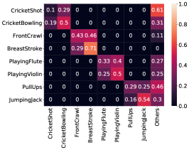
(a)

(b)

(c)

(d)

Figure 6: Confusion matrices for 4 highly confused class-pairs from UCF101 classification models with (a) no pretraining, (b) IC pretraining, and (c) TCLR pretraining. (d) Classes illustrated with a sample frame. TCLR significantly improves over IC in distinguishing visually similar classes.

4.3 Temporal diversity helps video understanding

To study the impact of temporal feature diversity directly, we utilize self-supervised pre-trained models only to avoid influence of supervised fine-tuning. As shown in Fig 7, increasing from 1 clip to 10 clips per video, we observe that the pretraining strategies using temporal contrastive losses get significant performance gains (about 7-8% for each individual loss and 14.67% for TCLR) with increasing number of clips. Instance Contrastive pretraining which enforces temporal invariance in learned features of video, does not see a similar improvement. It is also worth noting that each of the LL and GL losses help in learning different types of temporal diversity which results in TCLR having bigger improvements relative to either of the temporal contrastive losses. Performance gains of a similar nature can also be observed in other downstream tasks as well, which are reported in Section F of the supplementary material.

Figure 7: Temporally distinct features learned by TCLR result in a significant improvement in NN-Retrieval on UCF101 (split-1) with increasing number of clips per video.

4.4 Distinguishing confusing class pairs

To examine the ability of TCLR to distinguish confusing classes, we looked at the most confused action class pairs for UCF101 action recognition models trained from scratch. We observe that the these pairs mostly consist of fine-grained variants of action classes, for example the swimming actions BreastStroke and FrontCrawl. Some such pairs of classes are visualized in Figure 6d. We can see that these classes are confusing because the corresponding frames are visually similar. In this study we considered a model without pretraining as a baseline, and tried to see the impact of instance contrastive and TCLR pretraining on it. We observe that despite a significant overall improvement in accuracy, instance contrastive pre-training does not provide any significant gain in distinguishing these confused class pairs over the scratch baseline. On the other hand, TCLR pre-training helps remarkably with the confused classes. Average recall for these 8 classes is 42.5% for the scratch model, 44.9% for the IC model and 74.8% for the TCLR model. Since the classes are visually similar, distinguishing them requires learning the temporal variation in videos.

5 Conclusion

In this work, we propose two novel Temporal Contrastive losses to improve the quality of learned self-supervised video representations over standard instance discrimination contrastive learning. We provide extensive experimental evidence on three diverse datasets and obtain state-of-the-art results across various downstream video understanding tasks. The success of our approach underscores the benefits of contrastive learning beyond instance discrimination.

Appendix A Supplementary Overview

The supplementary material is organized into the following sections:

• Section B: Dataset details

• Section C: Implementation details such as network architectures, data augmentations, self supervised training details (losses, optimizers, etc) and and downstream task evaluation protocols.

• Section D: Results for additional ablation experiments, to assess the impact of augmentation types, projection head design and loss hyperparameters on performance.

• Section E: Comparison of our instance contrastive and random initialization baseline with results reported in prior work

• Section F: Effect of temporal diversity on downstream tasks

• Section G: Additional results from prior work which were excluded from the main paper

• Section H: Feature slice similarity matrix of the learned representation

• Section I: Qualitative results of NN-Retrieval

• Section J: tSNE visualization of learned features and comparison with baselines

• Section K: Visualization of model attention

• Section L: Detailed comparison with the most relevant recent prior works

Appendix B Datasets

UCF101 [51] is the most commonly used dataset for the action recognition task. UCF101 has around 13,320 videos representing 101 different human activities.

Kinetics400 [10] is a large-scale human action recognition dataset having having 400 action classes summing up to 222,454 training videos at the time of our download.

HMDB51 [36] is a relatively smaller action recognition having around 7,000 total videos collected from 51 different human actions.

Appendix C Implementation Details

C.1 Network Architecture

We use the implementation of 3D-ResNet-18, R(2+1)D-18 and C3D provided by authors of prior works [63, 70, 66]. For 3D-ResNet and R(2+1)D, to get a feature map with temporal dimension 4 at the end of the penultimate layer, we change the temporal stride of the conv5 layer to 1, and the dilation factor to 2 in order to keep the temporal receptive field the same, while increasing the temporal resolution of the features. We spatially pool the feature map only after the penultimate layer which results in an encoded feature of dimension $4\times 512$ where 4 is temporal dimension and 512 is number of channels.

The MLP projection head consists of 2 layers in the default setting: Linear($512$, $512$) with ReLU activation and Linear($512$, $128$) followed by L2-Normalization. We use the 128-D output as representation vector to compute losses. We use shared weights for the 3D-CNN backbone and MLP across computation of different losses.

C.2 Augmentation

The augmentations we use for reporting benchmark scores are standard and prior methods also utilize similar augmentation strategies. We apply augmentation transformations from two broad categories: (1) Appearance based transforms and (2) Geometry based transforms.

Geometry based transforms Basic geometry-based augmentations include random scaling, random cropping, random cut-out and random horizontal-flip (details in Algorithm 1). Apart from basic augmentations, we also try the use of shear and rotation transformation with a small range (details in Section D), however for our benchmark results we only use basic augmentations.

Appearance based transforms Basic appearance-based transforms include random grayscale, random color drop, and color jittering with HSV color space (details in Algorithm 1). We also experiment with using Gaussian blurring filter (details in Section D), but we don’t use it for our reported results.

Each augmentation is applied with a certain probability and random strength selected from a specified interval. The exact same augmentation is applied on each frames of a video clip to ensure temporal consistency. Our augmentation pipeline is explained in Algorithm 1.

Input: Frames $F$, Output: Transformed Frames $F^{\prime}$ /* Random Resized Crop */

1 $w$, $h$ = dimensions($F$)

2 Generate $scale\sim\mathcal{U}(0.6,\,1.0)$

3 Generate $s_{x}\sim\mathcal{U}(0,\,1),\,s_{y}\sim\mathcal{U}(0,\,1)$

4 $x_{0},\,y_{0}=s_{x}\times(w-w\times scale),\,s_{y}\times(h-h\times scale)$

5 $x_{1},\,y_{1}=x_{0}+scale\times w,\,y_{0}+scale\times h$

6 $F^{\prime}=F$.spatial_crop$(x_{0},y_{0},x_{1},y_{1})$.resize$(112,112)$

/* Random contrast */

7 Generate $p_{0}\sim\mathcal{U}(0,\,1)$

8 if $p_{0}<0.25$ then

9       Generate $m_{0}\sim\mathcal{U}(0.75,\,1.25)$

10       $F^{\prime}$ = $F^{\prime}$.adjust_contrast($m_{0}$)

11      

/* Random Hue */

12 Generate $p_{1}\sim\mathcal{U}(0,\,1)$

13 if $p_{1}<0.3$ then

14       Generate $m_{1}\sim\mathcal{U}(-0.1,\,0.1)$

15       $F^{\prime}$ = $F^{\prime}$.adjust_hue($m_{1}$)

16      

/* Random Saturation */

17 Generate $p_{2}\sim\mathcal{U}(0,\,1)$

18 if $p_{2}<0.3$ then

19       Generate $m_{2}\sim\mathcal{U}(0.75,\,1.25)$

20       $F^{\prime}$ = $F^{\prime}$.adjust_saturation($m_{2}$)

21      

/* Random Brightness */

22 Generate $p_{3}\sim\mathcal{U}(0,\,1)$

23 if $p_{3}<0.3$ then

24       Generate $m_{3}\sim\mathcal{U}(0.75,\,1.25)$

25       $F^{\prime}$ = $F^{\prime}$.adjust_brightness($m_{3}$)

26      

/* Color Dropping */

27 Generate $p_{4}\sim\mathcal{U}(0,\,1)$

28 if $p_{4}>0.7$ then

29       if $p_{4}<0.875$ then

30             $F^{\prime}$ = $F^{\prime}$.to_grayscale()

31             Generate $p_{5}\sim\mathcal{U}(0,\,1)$

32             if $p_{5}<0.75$ then

33                   Generate $m_{4}\sim\mathcal{U}(0.75,\,1.25)$

34                   $F^{\prime}$ = $F^{\prime}$.adjust_gamma($m_{4}$)

35                  

36            

37      else

38             $F^{\prime}$ = $F^{\prime}$.drop_random_channel()

39            

40      

/* Random Horizontal Flip */

41 Generate $p_{6}\sim\mathcal{U}(0,\,1)$

42 if $p_{6}<0.5$ then

43       $F^{\prime}$ = $F^{\prime}$.horizontal_flip()

44      

/* Random Erase */

45 Generate $p_{7}\sim\mathcal{U}(0,\,1)$

46 if $p_{7}<0.5$ then

47       Generate $e_{x}\sim 112\times\mathcal{U}(0,\,1),\,e_{y}\sim 112\times\mathcal{U}(0,\,1)$

48       Generate $escale_{x},\,escale_{y}\sim 20\times\mathcal{U}(0.5,\,1)$

49       $F^{\prime}$ = $F^{\prime}$.erase($e_{x},\,e_{y},\,escale_{x},\,escale_{y}$)

50      

Algorithm 1 TCLR self-supervised training data augmentation.

C.3 Self-supervised training

The model for self-supervised pretraining consists of a backbone architecture combined with an MLP projection head. The loss is computed using the embedding from the final layer of the MLP. We use an input clip resolution of $112\times 112$ and 16 frames. From a set of 64 consecutive frames, the global clip is composed of 16 frames sampled with a skip rate of 4, whereas the 4 local clips also have 16 frames but are sampled with a skip rate of 1. We train our model by combining all loss terms with batch size of $40$ as shown in Equation 5, where, $N_{B}$ is the size of mini-batch, $\mathcal{L}_{IC}$ is the instance contrastive loss, $\mathcal{L}_{LL}$ is the local-local temporal contrastive loss and $\mathcal{L}_{GL}$ is the global-local temporal contrastive loss.

$$\mathcal{L}=\sum_{i=1}^{N_{B}}\mathcal{L}_{IC}^{i}+\mathcal{L}_{LL}^{i}+\mathcal{L}_{GL}^{i},$$ (5)

Figure 8 shows the values of different losses as the training progresses. We run the self-supervised pretraining for 400 epochs for UCF101 and 100 epochs for pretraining of Kinetics400. We use Adam [34] optimizer with $\beta_{1}=0.9,\beta_{2}=0.999,\epsilon=10^{-8}$, the default parameters for PyTorch v1.6.0. We use an initial learning of $0.001$ and decay the learning rate by a factor of 10 when the loss plateaus. We also use linear warm-up for the first 10 epochs.

As mentioned in Table-1 of the main paper, we reproduce results of CVRL for the commonly used configuration (model depth = 18, input frames = 16, resolution = $112\times 112$). In our replication, we use the exact same temporally consistent augmentations and temporal interval sampler $P(t)\propto-t+c$. Pretraining is done on UCF101 split-1 training set with batch size of 512 for 800 epochs.

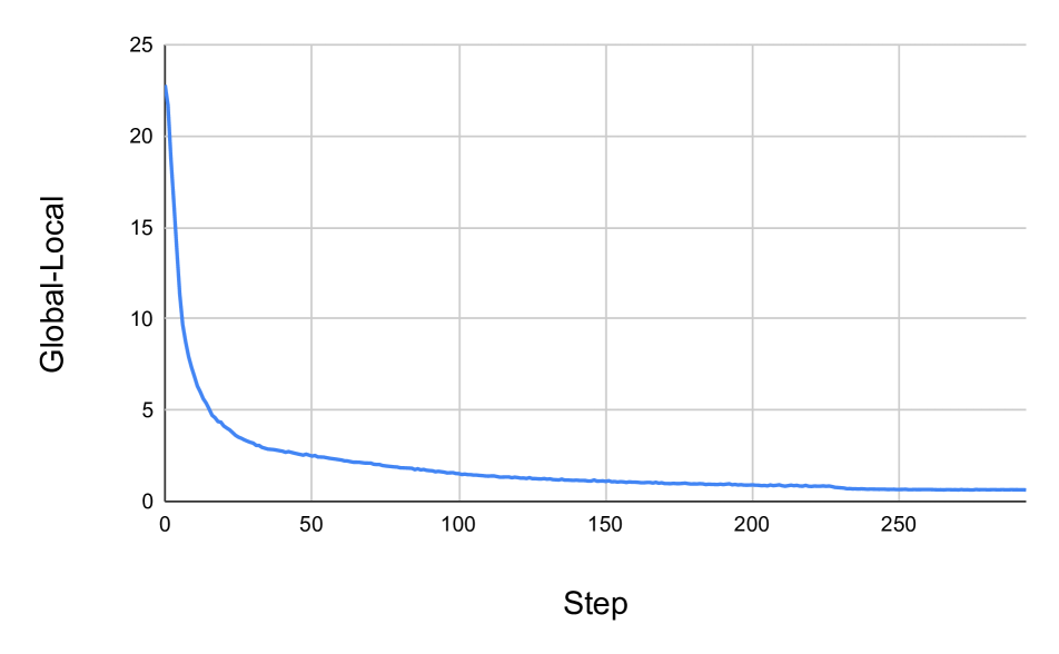
(a) Global-Local

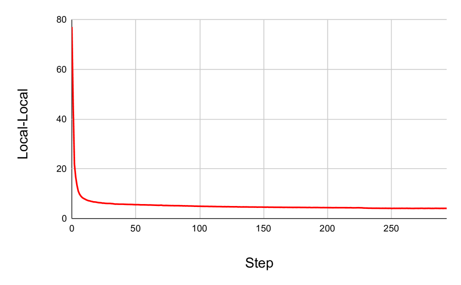
(b) Local-Local

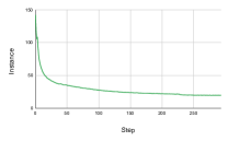
(c) Instance

Figure 8: Values of contrastive losses during progression of self-supervised pre-training.

C.4 Downstream Task Protocols

We evaluate self-supervised pretrained model for three downstream tasks: Action Recognition, Nearest Neighbor Video Retrieval, and Label Efficiency.

Action Recognition: For the action recognition task we follow the protocol used in prior works [30, 24, 63, 23, 56]. We attach a fully-connected layer (randomly initialized) to the pretrained video encoder and train all layers of the model using the training data with a cross-entropy loss. Following the prior works, we also utilize basic augmentations such as random crop, random scale and horizontal flip while training. These augmentations are standard for action recognition training [26, 58]. For the testing, we sample 10 uniformly spaced clips from the video average their predictions to get a video-level prediction. We utilize input clips of $112\times 112$ resolution and 16 frames with a skip rate of 2. A base learning rate of $0.001$ is used, which decreases by a factor of 10 on loss plateau. Linear warm-up starting from minimum learning rate of $0.00001$ and rising to base Learning Rate of $0.001$ is used for the first 10 epochs of the training.

Label Efficiency/ Finetuning with limited data: We use the same experimental setting as used for action recognition task and train with limited training data. For each limited fraction of training data, we repeat the experiment 3 times with different randomly sampled training-subsets and report average result.

Nearest Neighbor Video Retrieval: In this task, we directly use the self-supervised pretrained video encoder without further supervised finetuning. In the paper we report results using features from the final layer of the encoder with spatial pooling and averaged over 10 uniformly spaced clips from each video as followed by prior work [24].

Appendix D Additional Ablations

We perform additional ablations using 3D-ResNet-18 with self-supervised pretraining on UCF101 training set (split-1) and linear evaluation on UCF101 test set (split-1).

D.1 Impact of losses

In the main paper, we carry out ablation studies to measure the impact of each of our novel loss functions on the downstream tasks. A more complete set of results for these experiments are presented in Tables 5, 6 and 7.

Method	Recall@1	Recall@5	Recall@10	Recall@20
IC	40.76	56.41	65.33	74.44
IC+LL	51.1	67.83	74.57	80.89
IC+GL	47.32	63.10	71.42	78.72
TCLR	56.17	72.16	79.01	85.30

Table 5: Nearest Neighbor Video Retrieval on UCF101 using self-supervised R3D-18 models pretrained on UCF101 videos.

Method	Recall@1	Recall@5	Recall@10	Recall@20
IC	14.38	35.62	48.37	61.57
IC+LL	19.07	42.42	54.97	69.35
IC+GL	18.43	41.70	53.59	67.19
TCLR	22.75	45.36	57.84	73.07

Table 6: Nearest Neighbor Video Retrieval on HMDB51 using self-supervised R3D-18 models pretrained on UCF101 videos.

Method	1%	10%	20%	50%
Scratch	6.13	32.10	44.39	57.35
IC	22.86	53.91	60.26	65.74
LL + GL	9.78	48.66	59.45	68.64
IC + LL	26.43	63.09	69.68	73.53
IC + GL	23.93	60.16	67.40	72.34
TCLR	26.90	66.08	73.41	76.68

Table 7: Top-1 Accuracy after limited label finetuning of self-supervised R3D-18 models pretrained on UCF101 (split-1) videos.

D.2 Augmentation Types

We perform an ablation study to measure the impact of computationally expensive transformations (specifically random Gaussian Blurring, Shearing and Rotation). We observe (Results in Table 8) that adding these transforms only has a small effect on the performance of the model on downstream tasks, and removing them can reduce training time by as much as 30%. In these augmentation ablations, we use Gaussian blur with 30% probability, kernel size $(15,15)$ and standard deviation selected randomly from $(0,0.5)$ interval. We apply shear and rotation with 30% probability, with rotation angles selected randomly from $(-20^{\circ},20^{\circ})$. Even though it’s possible to obtain slightly better results by using blur and other complex augmentations we do not use them for our main reported results.

Transforms
Appearance	Geometric	Linear Evaluation (Top-1 Accuracy)
Basic	Basic	69.91
+ Blur	Basic	70.7 (+0.8)
Basic	+ Shear & Rotate	70.2 (+0.3)

Table 8: Effect of using additional transformations.

D.3 Embedding Size

It has previously been reported that the size of the embedding doesn’t have a significant effect [12] on image self supervised learning. In our experiments we observe that using a large embedding size typically results in slightly better performance, as reported in Table 9. The main paper utilizes embedding of 128.

Embedding size	Linear Evaluation (Top-1 Accuracy)
128	69.91
256	70.12 (+0.21)
512	70.63 (+0.72)

Table 9: Effect of embedding size.

D.4 Number of Timesteps

A key hyperparameter for the Temporal Constrastive losses is the number of Timesteps $(N_{T})$ that a given video instance is sliced into. Apart from the default setting of $N_{T}=4$ we also study $N_{T}=2$ and find that it degrades performance. We do not use higher values of $N_{T}$ since that causes a significant increase in amount of GPU memory and computation required. Results are available in Table 10.

Timesteps $(N_{T})$	Linear Evaluation (Top-1 Accuracy)
4	69.91
2	66.60 (-3.31)

Table 10: Effect of timesteps used in temporal contrastive losses.

D.5 Skip Rate

For the instance contrastive loss we generally use the same skip rate for both the anchor and pairing clip. We try using different skip rates (selected from $\{4,8,12,16\}$), but this results in a performance degradation of about 2.3% over the baseline.

For the Global-Local Temporal contrastive loss, we use a fixed skip rate of 4 for the global clips and a skip rate of 1 for the local clips. We perform an additional experiment, where we randomly select a skip rate for the Global clip from this set: $\{4,8,12,16\}$. We set the skip rate for the local clip to $1/4^{th}$ of the selected skip rate for global clip. This leads to a 2.6% degradation from the fixed skip rate baseline.

D.6 Contrastive Loss Temperature

Prior works [12, 49, 63] demonstrate that a temperature of about $0.1$ is optimal for instance contrastive losses. We try different settings (Results in Table 11) to discover the optimal temperature for the temporal contrastive losses. We discover that $0.1$ is a good choice, and also that having it set to be higher than the temperature for the instance contrastive loss is very important. Setting the temperature for temporal contrastive loss lower than the instance contrastive loss leads to significantly poor performance (right of the origin in the chart), as can be seen in Figure 9.

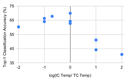
Figure 9: Effect of Contrastive Loss Temperature on downstream linear evaluation task. Using a lower temperature for temporal contrastive loss relative to the instance contrastive loss leads to poor results, as can seen from the right side of the origin in the chart.

$\mathcal{L}_{IC}$  Temperature	$\mathcal{L}_{LL}$, $\mathcal{L}_{GL}$  Temperature	Linear Evaluation  (Top-1 Accuracy)
0.01	0.01	62.75
0.01	0.1	64.03
0.01	1	60.32
0.05	0.05	64.28
0.1	0.01	44.22
0.1	0.1	69.93
0.1	0.5	67.78
0.1	1	66.33
1	0.01	40.93
1	0.1	51.10

Table 11: Effect of temperatures used in contrastive losses.

Appendix E Baseline Verification

Instance Contrastive Baseline: Our instance contrastive baseline using similar model architectures and input clip resolution ($112\times 112$, 16 frames) achieves 71.3% . We use the same input size, architecture and data augmentations for our instance contrastive baseline and TCLR model.

To ensure our instance contrastive baseline is correctly trained we also provide results from prior works in Table 13

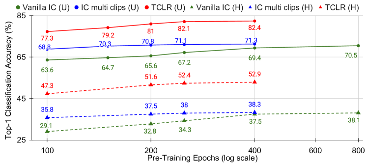
Figure 10: Effect of UCF101 pre-training duration on downstream UCF101 and HMDB51 action recognition. TCLR outperforms the Vanilla IC baseline with 4-8$\times$ times longer pre-training. (U) $\rightarrow$ UCF101 finetuning and (H) $\rightarrow$ HMDB51 finetuning

Method	Epochs	UCF	HMDB
IC [50]	200	70.0	39.9
IC [44]	300	69.5	-
IC [7]	200$\ast$	73.0	40.6
TCLR	50	82.2	51.9
TCLR	100	84.1	53.6

Table 12: Comparison of TCLR vs Vanilla IC with longer pre-training on Kinetics400 as reported in prior work.
$\ast$ email from authors

Source	Architecture	Pretrain	UCF101/HMDB51
Our $\mathcal{L}_{IC}$	R3D18	UCF101	71.3/ 38.3
[63]	R(2+1)D18	UCF101	67.3/ 28.6
[56]	R3D18	K400	70.0/ 39.9
[50]	R3D18	K400	69.5/ $-$
[5]	R3D18	K400	73.0/ 40.6

Table 13: Instance Contrastive baselines reported in prior work match our baseline results.

Random Initialization Baseline: Our baseline results with random initialization UCF101 finetuning (Top-1 classification accuracy 62.3%) which matches the prior results reported in [24] (61.8%). We report this random initialization baseline in Table 4 of the main paper along with other downstream tasks.

Appendix F Benefit of Temporal Diversity

We discussed the effects of temporal diversity on NN-Retrieval task for UCF101 in the main paper and found that increased temporal diversity leads to an increased gap with respect to the IC baseline in the multi-clip setting. Here we provide similar results for other downstream tasks and datasets. Detailed results across 10 different clip counts for UCF101 linear evaluation can be seen in Figure 11 and HMDB51 nearest neighbour retrieval can be seen in Figure 12. Summary results for 1 and 10 clip evaluation for 5 different tasks can be seen in Table 14.

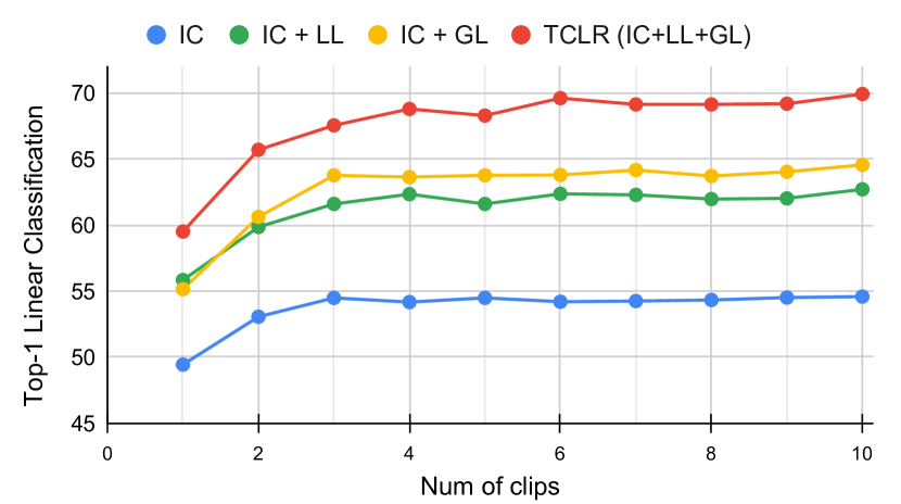
Figure 11: Temporally distinct features learned by TCLR result in a significant improvement in Linear Evaluation on UCF101 (split-1) with increasing number of clips per video.

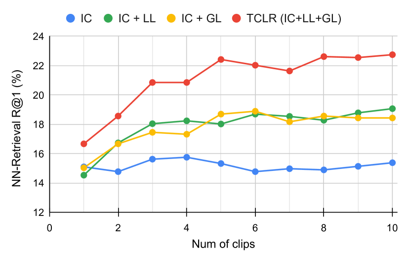
Figure 12: Temporally distinct features learned by TCLR result in a significant improvement in NN Retrieval on HMDB51 with increasing number of clips per video.

	UCF101			HMDB51
	Linear Eval	Finetuning	NN-Retrieval	Finetuning	NN-Retrieval
Scratch	14.80/ 17.15 (+2.35)	56.85/ 62.30 (+5.45)	8.21/ 9.77 (+1.56)	21.91/ 26.95 (+5.04)	4.77/ 4.05 (-0.72)
IC	49.43/ 54.58 (+5.15)	63.41/ 68.99 (+5.58)	38.52/ 40.76 (+2.24)	33.39/ 38.32 (+4.93)	15.1/ 15.38 (+0.28)
IC + LL	55.83/ 62.70 (+6.87)	66.85/ 74.38 (+7.53)	43.64/ 51.10 (+7.46)	42.80/ 49.77 (+6.96)	14.53/ 19.07 (+4.54)
IC + GL	55.14/ 64.55 (+9.41)	68.96/ 75.44 (+6.48)	38.54/ 47.32 (+8.78)	39.67/ 47.87 (+8.20)	15.03/ 18.43 (+3.4)
TCLR	59.50/ 69.91 (+10.41)	71.73/ 81.10 (+9.37)	41.50/ 56.17 (+14.67)	41.37/ 52.80 (+11.48)	16.67/ 22.75 (+6.08)

Table 14: Effect of using multiple clips on different evaluation results. 1-clip/ 10-clip performance on different downstream tasks.

Appendix G Additional Comparison

Results from prior work which were excluded from the main paper are presented in Table 15. The Table is divided into 3 sections. The first section includes results from papers which utilize visual modality but only provide results on specialized architectures or larger input sizes which are not widely used and hence cannot be compared fairly with other methods. The second section includes works which utilize multi-modal data, beyond the visual domain, such as text and audio. The third section shows our results for temporal contrastive learning from the main paper to allow for comparison with these works, such a comparison however is not fair for reasons explained earlier. We also perform linear classification of Kinetics-400 using our self-supervised pre-trained R2+1D model, which gives 21.8% top-1 accuracy.

Method	$\mathbf{H/W\times T}$	Backbone	Modality	Params ($\times 10^{6}$)	Pretraining	UCF101 finetune	HMDB51 finetune
Specialized Architectures
DVIM [67]	$-\times-$	R2D-18∗	V	-	UCF101	62.1	28.2
DVIM [67]	$-\times-$	R2D-18∗	V	-	K400	64.0	29.7
TCE [35]	$224\times-$	R2D50	V	23.0	K400	71.2	36.6
O3N [20]	$227\times-$	AlexNet	V	61.0	UCF101	60.3	32.5
Shuffle-Learn [44]	$227\times-$	AlexNet	V	61.0	UCF101	50.2	18.1
Büchler et al. [8]	$227\times-$	AlexNet∗	V	-	UCF101	58.6	25.0
Video Jigsaw [2]	$224\times 25$	CaffeNet	V	61.0	UCF101	46.4	-
Video Jigsaw [2]	$224\times 25$	CaffeNet	V	61.0	K400	55.4	27.0
CBT [3]	$112\times 16$	S3D	V	20.0	K600	79.5	44.6
Multi-Modal Methods
AVTS [47]	$224\times 25$	I3D	V+A	-	K400	83.7	53.0
AVTS [47]	$224\times 25$	MC3	V+A	-	AudioSet	89.0	61.6
MIL-NCE [43]	$224\times-$	S3D	V+T	-	HowTo100M	91.3	61.0
GDT [47]	$112\times 32$	R(2+1)D	V+A	-	K400	89.3	60.0
GDT [47]	$112\times 32$	R(2+1)D	V+A	-	IG65M	95.2	72.8
XDC [47]	$224\times 32$	R(2+1)D	V+A	-	K400	84.2	47.1
TCLR
TCLR (Ours)	$112\times 16$	R3D-18	V	13.5	UCF101	82.4	52.9
TCLR (Ours)	$112\times 16$	R3D-18	V	13.5	K400	84.1	53.6
TCLR (Ours)	$112\times 16$	R(2+1)D	V	14.4	UCF101	82.8	53.6
TCLR (Ours)	$112\times 16$	R(2+1)D	V	14.4	K400	84.3	54.2
TCLR (Ours)	$112\times 16$	C3D	V	27.7	UCF101	76.1	48.6

Table 15: Additional Finetuning Results (average of 3 splits) for action classification on UCF101 and HMDB51 from prior work that were excluded from the main paper, along with our results for comparison. Please note that these results are not strictly comparable since the prior work uses specialized architectures and larger input sizes, which has significant effect on performance and require excessive computational resources. V denotes Video(RGB) modality, A denotes audio, and T denotes text modality. ${}^{\ast}-$ modified architecture

Appendix H Feature Slice Representation Similarity

The goal of this visualization (see Figure 13 is to verify if the model learns temporal diversity in the feature map as intended by the TCLR framework. With a long global clip (16 frames with a skip rate of 4, hence covering 64 frames), representations for 4 different timesteps of the video feature map were obtained using the video encoder and projection head. Cosine similarity was computed between timesteps for each video and then averaged across the dataset. As can be observed, $\mathcal{L}_{GL}$ has the maximum impact on increasing within clip feature diversity, while $\mathcal{L}_{LL}$ also induces more diversity than the IC baseline.

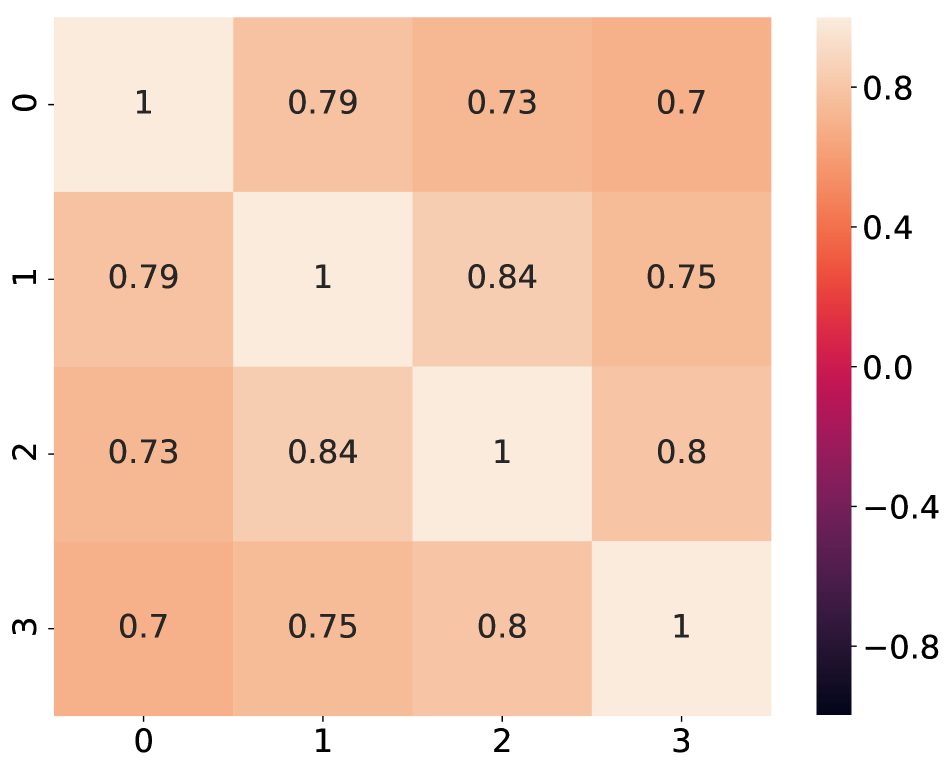
(a) Random Initialization

(b) $\mathcal{L}_{IC}$

(c) $\mathcal{L}_{IC}$ + $\mathcal{L}_{LL}$

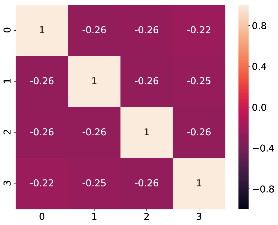
(d) $\mathcal{L}_{IC}$ + $\mathcal{L}_{GL}$

(e) TCLR

Figure 13: Cosine similarity between timesteps of the feature map learned using different losses. It can be observed that temporal distinctiveness learned features increases with the addition of temporal contrastive losses.

Appendix I Qualitative: Nearest Neighbour Retrieval

Qualitative results for nearest neighbour retrieval task on UCF101 are presented in Figure 14. These results are obtained using self-supervised pretrained models, without any supervised training with labels.

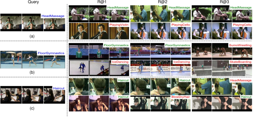
Figure 14: Qualitative Results: Nearest Neighbour Video Retrieval results on UCF101. For each query, the upper row show videos retrieved by our method and the lower row shows results from standard instance contrastive loss.

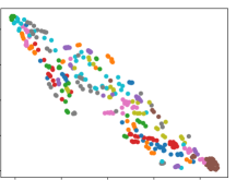
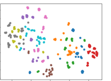
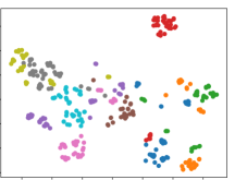
Figure 15: t-SNE visualization of Randomly Initialized (left) features; features learned using Instance Contrastive loss (center); and TCLR (right), for 10 randomly chosen action classes from UCF101 Test set: FieldHockeyPenalty, GolfSwing, SoccerJuggling, SoccerPenalty, PlayingGuitar, PlayingPiano, PlayingSitar, ApplyEyeMakeup, ApplyLipstick and BlowDryHair. TCLR results in more coherent clusters compared to the instance contrastive lossand is able to discriminate between similar classes with fine-grained differences such as ApplyEyeMakeup, ApplyLipstick and BlowDryHair.

Appendix J Visualization of Learned Representations

We use t-SNE [59] to visualize and study the representation learned by the model during self-supervised pre-training (without any supervised finetuning). We compare our method to the standard instance contrastive pretraining and randomly initialized features for a selected set of classes in Figure 15 for better visibility. In Figure 16 we compare TCLR to standard instance contrastive training for different sets of classes are selected at random to get a broad look at the overall representation space. The training set (split-1) of UCF101 without labels is used for pre-training and the test set is used for visualization. In order to ensure reproducible t-SNE results, we use PCA initialization and set perplexity to 50. As can be seen by comparing the representations, we can see that TCLR results in well separated clusters compared to the standard instance contrastive loss.

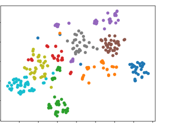
(a) MilitaryParade, TrampolineJumping, PlayingSitar, PlayingViolin, FieldHockeyPenalty, HighJump, StillRings, BlowDryHair, ApplyEyeMakeup

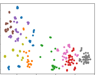
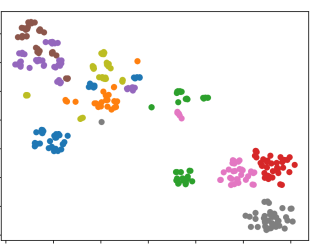
(b) PlayingSitar, PlayingPiano, GolfSwing, HighJump, ShavingBeard, ApplyLipstick, PoleVault, BasketballDunk, Typing, MixingBatter

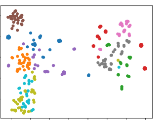
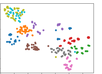
(c) FieldHockeyPenalty, HighJump, Knitting, Typing, Basketball, UnevenBars, ApplyLipstick, BlowDryHair, FrontCrawl, BreastStroke

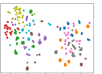
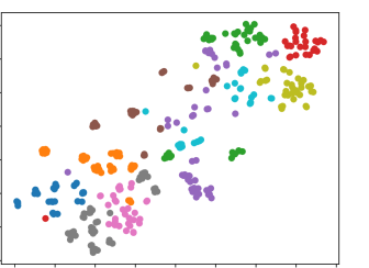
(d) Knitting, Typing, Diving, BreastStroke, HammerThrow, Nunchucks, Haircut, ShavingBeard, Biking, TrampolineJumping

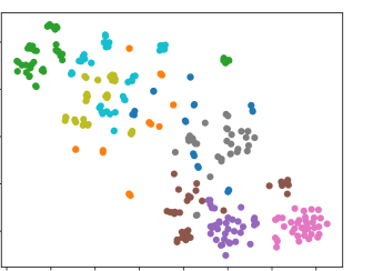
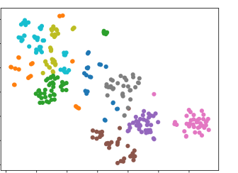
(e) PullUps, PushUps, WritingOnBoard, WalkingWithADog, HighJump, VolleyballSpiking, BasketballDunk, StillRings, BrushingTeeth, ShavingBeard

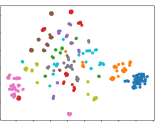
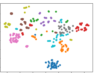
(f) BasketballDunk, ParallelBars, PlayingViolin, PlayingSitar, Knitting, Typing, WritingOnBoard, BlowingCandles, JumpingJack, HandstandWalking

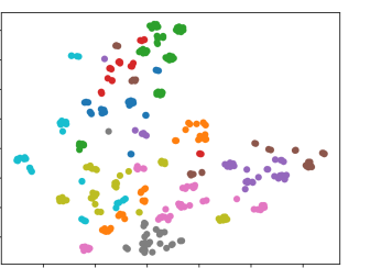
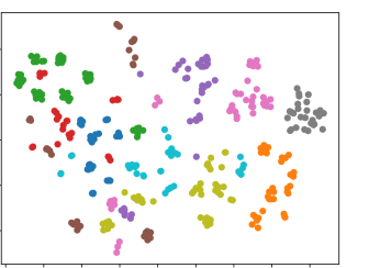
(g) WallPushups, Lunges, PlayingFlute, PlayingViolin, ParallelBars, PommelHorse, Diving, BreastStroke, Shotput, CricketBowling

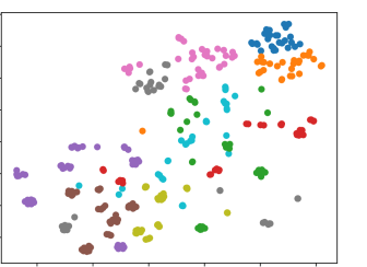
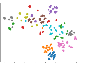
(h) Skijet, BreastStroke, Basketball, PommelHorse, PlayingSitar, PlayingDaf, FrisbeeCatch, GolfSwing, WallPushups, HandstandWalking

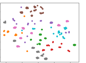
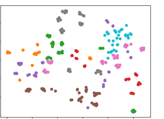
(i) HandstandPushups, WallPushups, Typing, Knitting, Archery, Shotput, PlayingDhol, PlayingFlute, WalkingWithADog, BlowingCandles

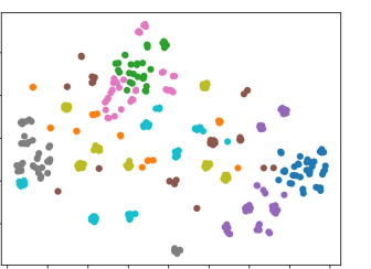
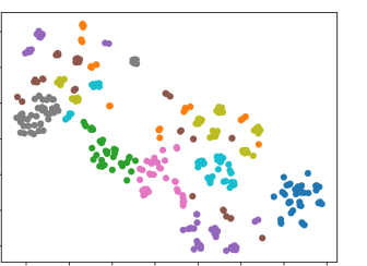
(j) Swing, BodyWeightSquats, CuttingInKitchen, MixingBatter, Shotput, Archery, BabyCrawling, WritingOnBoard, PlayingDhol, PlayingSitar

Figure 16: t-SNE visualization of representations learned using Instance Contrastive loss (left) and TCLR (right) of randomly chosen action classes from UCF101 Test set. In case of TCLR, we observe that the class boundaries are more compact and discriminative.

Appendix K Model Attention

In order to further examine the effect of TCLR pre-training on model performance, we use the method of Zagoruyko and Komodakis [71] to generate model attention for our method (from the fourth convolutional block of the R3D model) and compare it with the baseline supervised model. The qualitative samples are presented in Figures 17, 18, 19, and 20. We observe that the TCLR pre-trained model has significantly better focus on relevant portions of the video.

\begin{overpic}[width=243.46228pt]{suppfigs2/attention/52_comparison_BoxingSpeedBag_BoxingSpeedBag_BoxingSpeedBag_.png} \put(1.0,71.5){\hbox{\pagecolor{white}{\color[rgb]{0,0,1}\scriptsize BoxingSpeedBag}}} \put(1.0,46.75){\hbox{\pagecolor{white}{\color[rgb]{0.17254901960784313,0.6274509803921569,0.17254901960784313}\scriptsize BoxingSpeedBag}}} \put(1.0,22.0){\hbox{\pagecolor{white}{\color[rgb]{0.17254901960784313,0.6274509803921569,0.17254901960784313}\scriptsize BoxingSpeedBag}}} \end{overpic}

\begin{overpic}[width=243.46228pt]{suppfigs2/attention/1276_comparison_Fencing_Fencing_Fencing_.png} \put(1.0,71.5){\hbox{\pagecolor{white}{\color[rgb]{0,0,1}\scriptsize Fencing}}} \put(1.0,46.75){\hbox{\pagecolor{white}{\color[rgb]{0.17254901960784313,0.6274509803921569,0.17254901960784313}\scriptsize Fencing}}} \put(1.0,22.0){\hbox{\pagecolor{white}{\color[rgb]{0.17254901960784313,0.6274509803921569,0.17254901960784313}\scriptsize Fencing}}} \end{overpic}

\begin{overpic}[width=243.46228pt]{suppfigs2/attention/1290_comparison_Skiing_Kayaking_Skiing_.png} \put(1.0,71.5){\hbox{\pagecolor{white}{\color[rgb]{0,0,1}\scriptsize Skiing}}} \put(1.0,46.75){\hbox{\pagecolor{white}{\color[rgb]{0.8392156862745098,0.15294117647058825,0.1568627450980392}\scriptsize Kayaking}}} \put(1.0,22.0){\hbox{\pagecolor{white}{\color[rgb]{0.17254901960784313,0.6274509803921569,0.17254901960784313}\scriptsize Skiing}}} \end{overpic}

\begin{overpic}[width=243.46228pt]{suppfigs2/attention/1454_comparison_ApplyLipstick_ApplyLipstick_ApplyLipstick_.png} \put(1.0,71.5){\hbox{\pagecolor{white}{\color[rgb]{0,0,1}\scriptsize ApplyLipstick}}} \put(1.0,46.75){\hbox{\pagecolor{white}{\color[rgb]{0.17254901960784313,0.6274509803921569,0.17254901960784313}\scriptsize ApplyLipstick}}} \put(1.0,22.0){\hbox{\pagecolor{white}{\color[rgb]{0.17254901960784313,0.6274509803921569,0.17254901960784313}\scriptsize ApplyLipstick}}} \end{overpic}

\begin{overpic}[width=243.46228pt]{suppfigs2/attention/1622_comparison_Rowing_Skijet_Rowing_.png} \put(1.0,71.5){\hbox{\pagecolor{white}{\color[rgb]{0,0,1}\scriptsize Rowing}}} \put(1.0,46.75){\hbox{\pagecolor{white}{\color[rgb]{0.8392156862745098,0.15294117647058825,0.1568627450980392}\scriptsize Skijet}}} \put(1.0,22.0){\hbox{\pagecolor{white}{\color[rgb]{0.17254901960784313,0.6274509803921569,0.17254901960784313}\scriptsize Rowing}}} \end{overpic}

\begin{overpic}[width=243.46228pt]{suppfigs2/attention/1982_comparison_PizzaTossing_PizzaTossing_PizzaTossing_.png} \put(1.0,71.5){\hbox{\pagecolor{white}{\color[rgb]{0,0,1}\scriptsize PizzaTossing}}} \put(1.0,46.75){\hbox{\pagecolor{white}{\color[rgb]{0.17254901960784313,0.6274509803921569,0.17254901960784313}\scriptsize PizzaTossing}}} \put(1.0,22.0){\hbox{\pagecolor{white}{\color[rgb]{0.17254901960784313,0.6274509803921569,0.17254901960784313}\scriptsize PizzaTossing}}} \end{overpic}

Figure 17: Model attention: Ground-Truth Label on Video frames (Top Row), Attention for baseline fully supervised model (Middle Row) and Attention for TCLR pre-trained model(Bottom Row). We notice that for the TCLR pre-trained model the attention is more focused on action-centric regions.

\begin{overpic}[width=243.46228pt]{suppfigs2/attention/2052_comparison_Typing_Typing_Typing_.png} \put(1.0,71.5){\hbox{\pagecolor{white}{\color[rgb]{0,0,1}\scriptsize Typing}}} \put(1.0,46.75){\hbox{\pagecolor{white}{\color[rgb]{0.17254901960784313,0.6274509803921569,0.17254901960784313}\scriptsize Typing}}} \put(1.0,22.0){\hbox{\pagecolor{white}{\color[rgb]{0.17254901960784313,0.6274509803921569,0.17254901960784313}\scriptsize Typing}}} \end{overpic}

\begin{overpic}[width=243.46228pt]{suppfigs2/attention/2125_comparison_VolleyballSpiking_BasketballDunk_VolleyballSpiking_.png} \put(1.0,71.5){\hbox{\pagecolor{white}{\color[rgb]{0,0,1}\scriptsize VolleyballSpiking}}} \put(1.0,46.75){\hbox{\pagecolor{white}{\color[rgb]{0.8392156862745098,0.15294117647058825,0.1568627450980392}\scriptsize BasketballDunk}}} \put(1.0,22.0){\hbox{\pagecolor{white}{\color[rgb]{0.17254901960784313,0.6274509803921569,0.17254901960784313}\scriptsize VolleyballSpiking}}} \end{overpic}

\begin{overpic}[width=243.46228pt]{suppfigs2/attention/2130_comparison_VolleyballSpiking_Basketball_VolleyballSpiking_.png} \put(1.0,71.5){\hbox{\pagecolor{white}{\color[rgb]{0,0,1}\scriptsize VolleyballSpiking}}} \put(1.0,46.75){\hbox{\pagecolor{white}{\color[rgb]{0.8392156862745098,0.15294117647058825,0.1568627450980392}\scriptsize Basketball}}} \put(1.0,22.0){\hbox{\pagecolor{white}{\color[rgb]{0.17254901960784313,0.6274509803921569,0.17254901960784313}\scriptsize VolleyballSpiking}}} \end{overpic}

\begin{overpic}[width=243.46228pt]{suppfigs2/attention/2305_comparison_PlayingGuitar_PlayingGuitar_PlayingGuitar_.png} \put(1.0,71.5){\hbox{\pagecolor{white}{\color[rgb]{0,0,1}\scriptsize PlayingGuitar}}} \put(1.0,46.75){\hbox{\pagecolor{white}{\color[rgb]{0.17254901960784313,0.6274509803921569,0.17254901960784313}\scriptsize PlayingGuitar}}} \put(1.0,22.0){\hbox{\pagecolor{white}{\color[rgb]{0.17254901960784313,0.6274509803921569,0.17254901960784313}\scriptsize PlayingGuitar}}} \end{overpic}

\begin{overpic}[width=243.46228pt]{suppfigs2/attention/2439_comparison_SoccerJuggling_Shotput_SoccerJuggling_.png} \put(1.0,71.5){\hbox{\pagecolor{white}{\color[rgb]{0,0,1}\scriptsize SoccerJuggling}}} \put(1.0,46.75){\hbox{\pagecolor{white}{\color[rgb]{0.8392156862745098,0.15294117647058825,0.1568627450980392}\scriptsize Shotput}}} \put(1.0,22.0){\hbox{\pagecolor{white}{\color[rgb]{0.17254901960784313,0.6274509803921569,0.17254901960784313}\scriptsize SoccerJuggling}}} \end{overpic}

\begin{overpic}[width=243.46228pt]{suppfigs2/attention/2530_comparison_JugglingBalls_JugglingBalls_JugglingBalls_.png} \put(1.0,71.5){\hbox{\pagecolor{white}{\color[rgb]{0,0,1}\scriptsize JugglingBalls}}} \put(1.0,46.75){\hbox{\pagecolor{white}{\color[rgb]{0.17254901960784313,0.6274509803921569,0.17254901960784313}\scriptsize JugglingBalls}}} \put(1.0,22.0){\hbox{\pagecolor{white}{\color[rgb]{0.17254901960784313,0.6274509803921569,0.17254901960784313}\scriptsize JugglingBalls}}} \end{overpic}

Figure 18: Model attention (continued): Ground-Truth Label on Video frames (Top Row), Attention for baseline fully supervised model (Middle Row) and Attention for TCLR pre-trained model(Bottom Row). We notice that for the TCLR pre-trained model the attention is more focused on action-centric regions.

\begin{overpic}[width=243.46228pt]{suppfigs2/attention/2662_comparison_PlayingSitar_CuttingInKitchen_PlayingSitar_.png} \put(1.0,71.5){\hbox{\pagecolor{white}{\color[rgb]{0,0,1}\scriptsize PlayingSitar}}} \put(1.0,46.75){\hbox{\pagecolor{white}{\color[rgb]{0.8392156862745098,0.15294117647058825,0.1568627450980392}\scriptsize CuttingInKitchen}}} \put(1.0,22.0){\hbox{\pagecolor{white}{\color[rgb]{0.17254901960784313,0.6274509803921569,0.17254901960784313}\scriptsize PlayingSitar}}} \end{overpic}

\begin{overpic}[width=243.46228pt]{suppfigs2/attention/2920_comparison_FrontCrawl_FrontCrawl_FrontCrawl_.png} \put(1.0,71.5){\hbox{\pagecolor{white}{\color[rgb]{0,0,1}\scriptsize FrontCrawl}}} \put(1.0,46.75){\hbox{\pagecolor{white}{\color[rgb]{0.17254901960784313,0.6274509803921569,0.17254901960784313}\scriptsize FrontCrawl}}} \put(1.0,22.0){\hbox{\pagecolor{white}{\color[rgb]{0.17254901960784313,0.6274509803921569,0.17254901960784313}\scriptsize FrontCrawl}}} \end{overpic}

\begin{overpic}[width=243.46228pt]{suppfigs2/attention/3024_comparison_HeadMassage_PlayingTabla_HeadMassage_.png} \put(1.0,71.5){\hbox{\pagecolor{white}{\color[rgb]{0,0,1}\scriptsize HeadMassage}}} \put(1.0,46.75){\hbox{\pagecolor{white}{\color[rgb]{0.8392156862745098,0.15294117647058825,0.1568627450980392}\scriptsize PlayingTabla}}} \put(1.0,22.0){\hbox{\pagecolor{white}{\color[rgb]{0.17254901960784313,0.6274509803921569,0.17254901960784313}\scriptsize HeadMassage}}} \end{overpic}

\begin{overpic}[width=243.46228pt]{suppfigs2/attention/3089_comparison_Lunges_PizzaTossing_Lunges_.png} \put(1.0,71.5){\hbox{\pagecolor{white}{\color[rgb]{0,0,1}\scriptsize Lunges}}} \put(1.0,46.75){\hbox{\pagecolor{white}{\color[rgb]{0.8392156862745098,0.15294117647058825,0.1568627450980392}\scriptsize PizzaTossing}}} \put(1.0,22.0){\hbox{\pagecolor{white}{\color[rgb]{0.17254901960784313,0.6274509803921569,0.17254901960784313}\scriptsize Lunges}}} \end{overpic}

\begin{overpic}[width=243.46228pt]{suppfigs2/attention/3158_comparison_Mixing_CuttingInKitchen_Mixing_.png} \put(1.0,71.5){\hbox{\pagecolor{white}{\color[rgb]{0,0,1}\scriptsize Mixing}}} \put(1.0,46.75){\hbox{\pagecolor{white}{\color[rgb]{0.8392156862745098,0.15294117647058825,0.1568627450980392}\scriptsize CuttingInKitchen}}} \put(1.0,22.0){\hbox{\pagecolor{white}{\color[rgb]{0.17254901960784313,0.6274509803921569,0.17254901960784313}\scriptsize Mixing}}} \end{overpic}

\begin{overpic}[width=243.46228pt]{suppfigs2/attention/3308_comparison_Rafting_Rafting_Rafting_.png} \put(1.0,71.5){\hbox{\pagecolor{white}{\color[rgb]{0,0,1}\scriptsize Rafting}}} \put(1.0,46.75){\hbox{\pagecolor{white}{\color[rgb]{0.17254901960784313,0.6274509803921569,0.17254901960784313}\scriptsize Rafting}}} \put(1.0,22.0){\hbox{\pagecolor{white}{\color[rgb]{0.17254901960784313,0.6274509803921569,0.17254901960784313}\scriptsize Rafting}}} \end{overpic}

Figure 19: Model attention (continued): Ground-Truth Label on Video frames (Top Row), Attention for baseline fully supervised model (Middle Row) and Attention for TCLR pre-trained model(Bottom Row).We notice that for the TCLR pre-trained model the attention is more focused on action-centric regions.

\begin{overpic}[width=243.46228pt]{suppfigs2/attention/3365_comparison_SumoWrestling_SumoWrestling_SumoWrestling_.png} \put(1.0,71.5){\hbox{\pagecolor{white}{\color[rgb]{0,0,1}\scriptsize SumoWrestling}}} \put(1.0,46.75){\hbox{\pagecolor{white}{\color[rgb]{0.17254901960784313,0.6274509803921569,0.17254901960784313}\scriptsize SumoWrestling}}} \put(1.0,22.0){\hbox{\pagecolor{white}{\color[rgb]{0.17254901960784313,0.6274509803921569,0.17254901960784313}\scriptsize SumoWrestling}}} \end{overpic}

\begin{overpic}[width=243.46228pt]{suppfigs2/attention/3413_comparison_TableTennisShot_TableTennisShot_TableTennisShot_.png} \put(1.0,71.5){\hbox{\pagecolor{white}{\color[rgb]{0,0,1}\scriptsize TableTennisShot}}} \put(1.0,46.75){\hbox{\pagecolor{white}{\color[rgb]{0.17254901960784313,0.6274509803921569,0.17254901960784313}\scriptsize TableTennisShot}}} \put(1.0,22.0){\hbox{\pagecolor{white}{\color[rgb]{0.17254901960784313,0.6274509803921569,0.17254901960784313}\scriptsize TableTennisShot}}} \end{overpic}

\begin{overpic}[width=243.46228pt]{suppfigs2/attention/3747_comparison_ShavingBeard_ShavingBeard_ShavingBeard_.png} \put(1.0,71.5){\hbox{\pagecolor{white}{\color[rgb]{0,0,1}\scriptsize ShavingBeard}}} \put(1.0,46.75){\hbox{\pagecolor{white}{\color[rgb]{0.17254901960784313,0.6274509803921569,0.17254901960784313}\scriptsize ShavingBeard}}} \put(1.0,22.0){\hbox{\pagecolor{white}{\color[rgb]{0.17254901960784313,0.6274509803921569,0.17254901960784313}\scriptsize ShavingBeard}}} \end{overpic}

\begin{overpic}[width=243.46228pt]{suppfigs2/attention/379_comparison_PlayingCello_PlayingCello_PlayingCello_.png} \put(1.0,71.5){\hbox{\pagecolor{white}{\color[rgb]{0,0,1}\scriptsize PlayingCello}}} \put(1.0,46.75){\hbox{\pagecolor{white}{\color[rgb]{0.17254901960784313,0.6274509803921569,0.17254901960784313}\scriptsize PlayingCello}}} \put(1.0,22.0){\hbox{\pagecolor{white}{\color[rgb]{0.17254901960784313,0.6274509803921569,0.17254901960784313}\scriptsize PlayingCello}}} \end{overpic}

\begin{overpic}[width=243.46228pt]{suppfigs2/attention/506_comparison_CuttingInKitchen_BabyCrawling_CuttingInKitchen_.png} \put(1.0,71.5){\hbox{\pagecolor{white}{\color[rgb]{0,0,1}\scriptsize CuttingInKitchen}}} \put(1.0,46.75){\hbox{\pagecolor{white}{\color[rgb]{0.8392156862745098,0.15294117647058825,0.1568627450980392}\scriptsize BabyCrawling}}} \put(1.0,22.0){\hbox{\pagecolor{white}{\color[rgb]{0.17254901960784313,0.6274509803921569,0.17254901960784313}\scriptsize CuttingInKitchen}}} \end{overpic}

\begin{overpic}[width=243.46228pt]{suppfigs2/attention/1434_comparison_BaseballPitch_GolfSwing_BaseballPitch_.png} \put(1.0,71.5){\hbox{\pagecolor{white}{\color[rgb]{0,0,1}\scriptsize BaseballPitch}}} \put(1.0,46.75){\hbox{\pagecolor{white}{\color[rgb]{0.8392156862745098,0.15294117647058825,0.1568627450980392}\scriptsize GolfSwing}}} \put(1.0,22.0){\hbox{\pagecolor{white}{\color[rgb]{0.17254901960784313,0.6274509803921569,0.17254901960784313}\scriptsize BaseballPitch}}} \end{overpic}

Figure 20: Model attention (continued): Ground-Truth Label on Video frames (Top Row), Attention for baseline fully supervised model (Middle Row) and Attention for TCLR pre-trained model(Bottom Row). We notice that for the TCLR pre-trained model the attention is more focused on action-centric regions.

Appendix L Detailed comparison with recent prior work

We contrast our method with 6 recent works in the area: CVRL, TaCo, CoCLR, IIC, Video DeepInfoMax and SeCo.

L.1 CVRL [49]

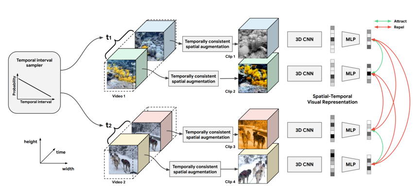
Figure 21: CVRL Framework from Qian et al. [49]

CVRL introduces the Temporal Interval Sampler, the key idea behind it being to not take positives from uniformly random timestamps from the same instance, rather take positives which close to each other temporally. CVRL improves upon standard instance contrastive learning by trying to avoid learning excessive temporal invariance while TCLR explicitly learns within-instance temporal distinctiveness by taking negatives from the same instance, and hence is an orthogonal approach to the problem of excessive temporal invariance.

L.2 TaCo [5]

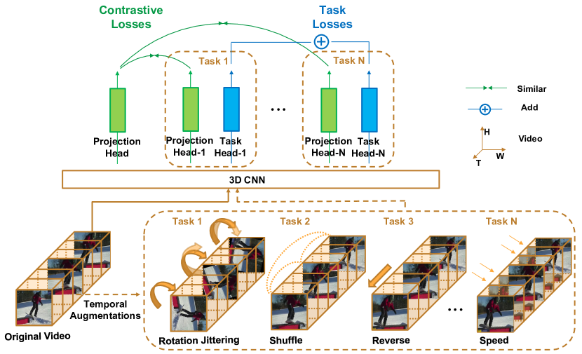
Figure 22: TaCo Framework from Bai et al. [5]

TaCo combines instance contrastive learning with multiple temporal pretext tasks (rotation, shuffled, reverse, or speed) in a multi-task setting in order to learn temporally varying features. The different tasks have their own projection and task heads, but share a common backbone. The TaCo approach to learning temporally distinct features is a differnt approach from TCLR, where we utilize temporal contrastive losses instead of any pretext tasks.

L.3 CoCLR [25]

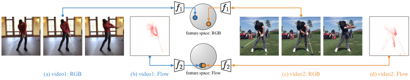
Figure 23: CoCLR Framework from Han et al. [25]

CoCLR introduces a multi-stage pretraining process that improves upon instance contrastive learning by mining positive pairs across instances in a cross-modal fashion, i.e. positive pairs mined from RGB modality are used for optical flow, and vice versa.

L.4 IIC [54]

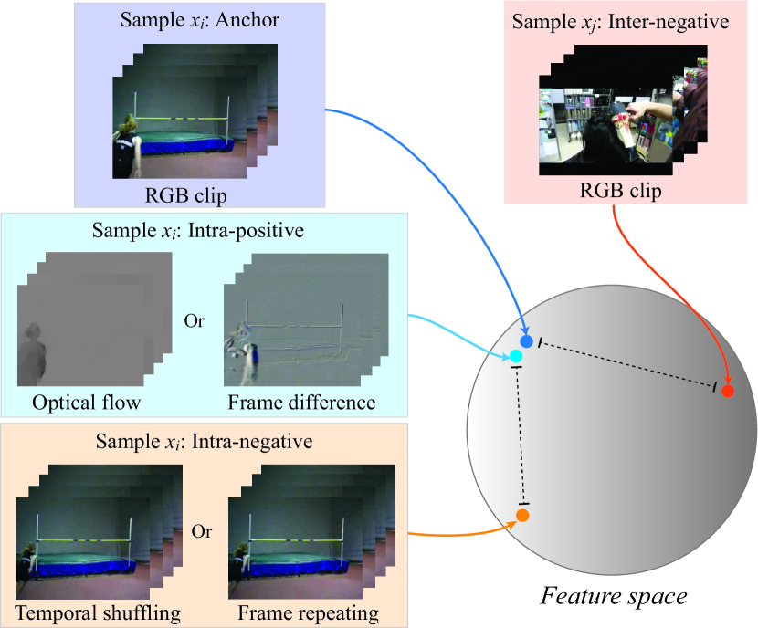
Figure 24: IIC Framework from Tao et al. [54]

IIC framework builds on the contrastive loss by utilizing positive pairs from different modalities (such as optical flow) and creating a new class of negatives by shuffling and repeating the anchor. Unlike TCLR’s $\mathcal{L}_{LL}$ loss, IIC does not use temporally distinct clips as negative pairs.

L.5 VideoDeepInfoMax [16]

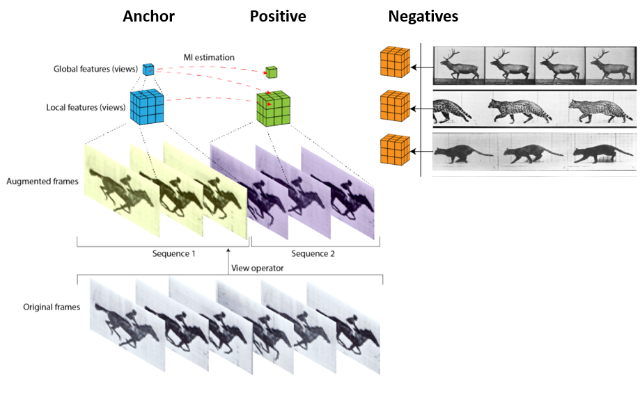
Figure 25: Video DIM Framework from Devon Hjelm and Bachman [25]

VideoDIM learns through instance discrimination using both local and global views of the features. Positive pairs are formed from local and global features of the same instance, whereas negative pairs are formed from local and global features of different instances.The local features are obtained from lower level convolutional layers, whereas the global feature comes from the final layer. Like other forms of instance discrimination based learning VideoDIM does not achieve temporal distinctiveness, and rather enforces invariance. Whereas, $\mathcal{L}_{GL}$ loss in TCLR promotes distinctiveness in the local features along the temporal dimension.

L.6 Comparison with SeCo [69]

SeCo combines multiple pretext tasks and its results cannot be compared with VideoSSL methods like TCLR which start from scratch; SeCo uses a 2D CNN initialized with ImageNet MoCov2 pre-trained weights. Moreover, most of the gain of SeCo over ImageNet trained initialization comes from instance contrastive loss and adding intra-frame loss in SeCo only results in gain of $\sim$1-2% across downstream tasks (Table 1 of [69]). Whereas with TCLR, gains across downstream tasks upon adding the Local-Local loss are significant ($\sim$6-11%, see Table 4 of the main paper). SeCo doesn’t include any temporal component (like 3D-Conv or RNN) in the backbone during the SSL phase; it uses 2D CNN and as a result their intra-frame contrastive loss only learns to discriminate visual appearance instead of spatio-temporal features.

References

- [1] Triantafyllos Afouras, Andrew Owens, Joon Son Chung, and Andrew Zisserman. Self-supervised learning of audio-visual objects from video. In The European Conference on Computer Vision, 2020.
- [2] Unaiza Ahsan, Rishi Madhok, and Irfan Essa. Video Jigsaw: Unsupervised learning of spatiotemporal context for video action recognition, pages 179–189. 2019.
- [3] Humam Alwassel, Dhruv Mahajan, Bruno Korbar, Lorenzo Torresani, Bernard Ghanem, and Du Tran. Self-Supervised Learning by Cross-Modal Audio-Video Clustering, pages 9758–9770. 2020.
- [4] Philip Bachman, R. Devon Hjelm, and William Buchwalter. Learning representations by maximizing mutual information across views. In Advances in Neural Information Processing Systems, pages 15535–15545, 2019.
- [5] Yutong Bai, Haoqi Fan, Ishan Misra, Ganesh Venkatesh, Yongyi Lu, Yuyin Zhou, Qihang Yu, Vikas Chandra, and Alan Yuille. Can temporal information help with contrastive self-supervised learning? arXiv preprint arXiv:2011.13046, 2020.
- [6] Nadine Behrmann, Jurgen Gall, and Mehdi Noroozi. Unsupervised video representation learning by bidirectional feature prediction. In Proceedings of the IEEE/CVF Winter Conference on Applications of Computer Vision, pages 1670–1679, 2021.
- [7] Sagie Benaim, Ariel Ephrat, Oran Lang, Inbar Mosseri, William T. Freeman, Michael Rubinstein, Michal Irani, and Tali Dekel. Speednet: Learning the speediness in videos. In Proceedings of the IEEE/CVF Conference on Computer Vision and Pattern Recognition, pages 9922–9931, 2020.
- [8] Uta Buchler, Biagio Brattoli, and Bjorn Ommer. Improving spatiotemporal self-supervision by deep reinforcement learning. In Proceedings of the European conference on computer vision (ECCV), pages 770–786, 2018.
- [9] Mathilde Caron, Ishan Misra, Julien Mairal, Priya Goyal, Piotr Bojanowski, and Armand Joulin. Unsupervised Learning of Visual Features by Contrasting Cluster Assignments, pages 9912–9924. 2020.
- [10] Joao Carreira and Andrew Zisserman. Quo vadis, action recognition? a new model and the kinetics dataset. In Proceedings of the IEEE Conference on Computer Vision and Pattern Recognition, pages 6299–6308, 2017.
- [11] Peihao Chen, Deng Huang, Dongliang He, Xiang Long, Runhao Zeng, Shilei Wen, Mingkui Tan, and Chuang Gan. Rspnet: Relative speed perception for unsupervised video representation learning. In The AAAI Conference on Artificial Intelligence, 2021.
- [12] Ting Chen, Simon Kornblith, Mohammad Norouzi, and Geoffrey Hinton. A simple framework for contrastive learning of visual representations. In ICML, 2020.
- [13] Hyeon Cho, Taehoon Kim, Hyung Jin Chang, and Wonjun Hwang. Self-supervised visual learning by variable playback speeds prediction of a video. IEEE Access, 9:79562–79571, 2021.
- [14] Jinwoo Choi, Chen Gao, Joseph C.E. Messou, and Jia-Bin Huang. Why can’t i dance in the mall? learning to mitigate scene bias in action recognition. In Advances in Neural Information Processing Systems, pages 853–865, 2019.
- [15] Ishan Dave, Naman Biyani, Brandon Clark, Rohit Gupta, Yogesh Rawat, and Mubarak Shah. ” knights”: First place submission for vipriors21 action recognition challenge at iccv 2021. arXiv preprint arXiv:2110.07758, 2021.
- [16] R Devon Hjelm and Philip Bachman. Representation learning with video deep infomax. arXiv preprint arXiv:2007.13278, 2020.
- [17] Ali Diba, Mohsen Fayyaz, Vivek Sharma, Manohar Paluri, Jürgen Gall, Rainer Stiefelhagen, and Luc Van Gool. Large scale holistic video understanding, pages 593–610. 2020.
- [18] Christoph Feichtenhofer, Haoqi Fan, Jitendra Malik, and Kaiming He. Slowfast networks for video recognition. In Proceedings of the IEEE International Conference on Computer Vision, pages 6202–6211, 2019.
- [19] Christoph Feichtenhofer, Haoqi Fan, Bo Xiong, Ross Girshick, and Kaiming He. A large-scale study on unsupervised spatiotemporal representation learning. In Proceedings of the IEEE/CVF Conference on Computer Vision and Pattern Recognition, pages 3299–3309, 2021.
- [20] Basura Fernando, Hakan Bilen, Efstratios Gavves, and Stephen Gould. Self-supervised video representation learning with odd-one-out networks. In Proceedings of the IEEE Conference on Computer Vision and Pattern Recognition, pages 3636–3645, 2017.
- [21] Kirill Gavrilyuk, Mihir Jain, Ilia Karmanov, and Cees GM Snoek. Motion-augmented self-training for video recognition at smaller scale. In Proceedings of the IEEE/CVF International Conference on Computer Vision, pages 10429–10438, 2021.
- [22] Michael Gutmann and Aapo Hyvärinen. Noise-contrastive estimation: A new estimation principle for unnormalized statistical models. In Proceedings of the Thirteenth International Conference on Artificial Intelligence and Statistics, pages 297–304, 2010.
- [23] Tengda Han, Weidi Xie, and Andrew Zisserman. Video representation learning by dense predictive coding. In Proceedings of the IEEE/CVF International Conference on Computer Vision (ICCV) Workshops, 2019.
- [24] Tengda Han, Weidi Xie, and Andrew Zisserman. Memory-augmented dense predictive coding for video representation learning, pages 312–329. 2020a.
- [25] Tengda Han, Weidi Xie, and Andrew Zisserman. Self-supervised Co-Training for Video Representation Learning, pages 5679–5690. 2020b.
- [26] K. Hara, H. Kataoka, and Y. Satoh. Towards good practice for action recognition with spatiotemporal 3d convolutions. In 2018 24th International Conference on Pattern Recognition, pages 2516–2521, 2018.
- [27] Kaiming He, Haoqi Fan, Yuxin Wu, Saining Xie, and Ross Girshick. Momentum contrast for unsupervised visual representation learning. In Proceedings of the IEEE/CVF Conference on Computer Vision and Pattern Recognition, pages 9729–9738, 2020.
- [28] Yuqi Huo, Mingyu Ding, Haoyu Lu, Zhiwu Lu, Tao Xiang, Ji-Rong Wen, Ziyuan Huang, Jianwen Jiang, Shiwei Zhang, Mingqian Tang, Songfang Huang, and Ping Luo. Self-supervised video representation learning with constrained spatiotemporal jigsaw, 2021.
- [29] Simon Jenni and Hailin Jin. Time-equivariant contrastive video representation learning. In Proceedings of the IEEE/CVF International Conference on Computer Vision, pages 9970–9980, 2021.
- [30] Simon Jenni, Givi Meishvili, and Paolo Favaro. Video representation learning by recognizing temporal transformations. In The European Conference on Computer Vision, 2020.
- [31] Longlong Jing, Xiaodong Yang, Jingen Liu, and Yingli Tian. Self-supervised spatiotemporal feature learning via video rotation prediction. arXiv preprint arXiv:1811.11387, 2018.
- [32] Hirokatsu Kataoka, Tenga Wakamiya, Kensho Hara, and Yutaka Satoh. Would mega-scale datasets further enhance spatiotemporal 3d cnns? arXiv preprint arXiv:2004.04968, 2020.
- [33] Dahun Kim, Donghyeon Cho, and In So Kweon. Self-supervised video representation learning with space-time cubic puzzles. In Proceedings of the AAAI Conference on Artificial Intelligence, vol. 33, pages 8545–8552, 2019.
- [34] Diederik P. Kingma and Jimmy Ba. Adam: A method for stochastic optimization. In Yoshua Bengio and Yann LeCun, editors, 3rd International Conference on Learning Representations, ICLR 2015, San Diego, CA, USA, May 7-9, 2015, Conference Track Proceedings, 2015.
- [35] Joshua Knights, Ben Harwood, Daniel Ward, Anthony Vanderkop, Olivia Mackenzie-Ross, and Peyman Moghadam. Temporally coherent embeddings for self-supervised video representation learning. In 2020 25th International Conference on Pattern Recognition (ICPR), pages 8914–8921. IEEE, 2021.
- [36] H. Kuehne, H. Jhuang, E. Garrote, T. Poggio, and T. Serre. Hmdb: a large video database for human motion recognition. In Proceedings of the International Conference on Computer Vision, 2011.
- [37] Hsin-Ying Lee, Jia-Bin Huang, Maneesh Singh, and Ming-Hsuan Yang. Unsupervised representation learning by sorting sequences. In Proceedings of the IEEE International Conference on Computer Vision, pages 667–676, 2017.
- [38] Attila Lengyel, Robert-Jan Bruintjes, Marcos Baptista Rios, Osman Semih Kayhan, Davide Zambrano, Nergis Tomen, and Jan van Gemert. Vipriors 2: Visual inductive priors for data-efficient deep learning challenges. arXiv preprint arXiv:2201.08625, 2022.
- [39] Yingwei Li, Yi Li, and Nuno Vasconcelos. Resound: Towards action recognition without representation bias. In Proceedings of the European Conference on Computer Vision, pages 513–528, 2018.
- [40] Guillaume Lorre, Jaonary Rabarisoa, Astrid Orcesi, Samia Ainouz, and Stephane Canu. Temporal contrastive pretraining for video action recognition. In The IEEE Winter Conference on Applications of Computer Vision, pages 662–670, 2020.
- [41] Dezhao Luo, Chang Liu, Yu Zhou, Dongbao Yang, Can Ma, Qixiang Ye, and Weiping Wang. Video cloze procedure for self-supervised spatio-temporal learning. In Proceedings of the AAAI Conference on Artificial Intelligence, vol. 33, pages 11701–11708, 2020.
- [42] Antoine Miech, Jean-Baptiste Alayrac, Lucas Smaira, Ivan Laptev, Josef Sivic, and Andrew Zisserman. End-to-end learning of visual representations from uncurated instructional videos. In Proceedings of the IEEE/CVF Conference on Computer Vision and Pattern Recognition, pages 9879–9889, 2020a.
- [43] Antoine Miech, Jean-Baptiste Alayrac, Lucas Smaira, Ivan Laptev, Josef Sivic, and Andrew Zisserman. End-to-end learning of visual representations from uncurated instructional videos. In Proceedings of the IEEE/CVF Conference on Computer Vision and Pattern Recognition, pages 9879–9889, 2020b.
- [44] Ishan Misra, C. Lawrence Zitnick, and Martial Hebert. Shuffle and learn: unsupervised learning using temporal order verification, pages 527–544. 2016.
- [45] Aaron van den Oord, Yazhe Li, and Oriol Vinyals. Representation learning with contrastive predictive coding. arXiv preprint arXiv:1807.03748, 2018.
- [46] Tian Pan, Yibing Song, Tianyu Yang, Wenhao Jiang, and Wei Liu. Videomoco: Contrastive video representation learning with temporally adversarial examples. In Proceedings of the IEEE/CVF Conference on Computer Vision and Pattern Recognition, pages 11205–11214, 2021.
- [47] Mandela Patrick, Yuki Asano, Polina Kuznetsova, Ruth Fong, Joao F. Henriques, Geoffrey Zweig, and Andrea Vedaldi. Multi-modal self-supervision from generalized data transformations, 2021.
- [48] Rui Qian, Yuxi Li, Huabin Liu, John See, Shuangrui Ding, Xian Liu, Dian Li, and Weiyao Lin. Enhancing self-supervised video representation learning via multi-level feature optimization. In Proceedings of the International Conference on Computer Vision, 2021.
- [49] Rui Qian, Tianjian Meng, Boqing Gong, Ming-Hsuan Yang, Huisheng Wang, Serge Belongie, and Yin Cui. Spatiotemporal contrastive video representation learning. In Proceedings of the IEEE/CVF Conference on Computer Vision and Pattern Recognition, pages 6964–6974, 2021.
- [50] Hao Shao, Yu Liu, and Hongsheng Li. Self-supervised temporal learning, 2021.
- [51] Khurram Soomro, Amir Roshan Zamir, and Mubarak Shah. Ucf101: A dataset of 101 human actions classes from videos in the wild. arXiv preprint arXiv:1212.0402, 2012.
- [52] Chen Sun, Fabien Baradel, Kevin Murphy, and Cordelia Schmid. Learning video representations using contrastive bidirectional transformer. arXiv preprint arXiv:1906.05743, 2019.
- [53] Tomoyuki Suzuki, Takahiro Itazuri, Kensho Hara, and Hirokatsu Kataoka. Learning spatiotemporal 3d convolution with video order self-supervision. In Proceedings of the European Conference on Computer Vision, 2018.
- [54] Li Tao, Xueting Wang, and Toshihiko Yamasaki. Self-supervised video representation learning using inter-intra contrastive framework. In Proceedings of the 28th ACM International Conference on Multimedia, pages 2193–2201, 2020.
- [55] Yuan Tian, Zhaohui Che, Wenbo Bao, Guangtao Zhai, and Zhiyong Gao. Self-supervised Motion Representation via Scattering Local Motion Cues, pages 71–89. 2020.
- [56] Pavel Tokmakov, Martial Hebert, and Cordelia Schmid. Unsupervised learning of video representations via dense trajectory clustering. In European Conference on Computer Vision, pages 404–421. Springer, 2020.
- [57] Du Tran, Lubomir Bourdev, Rob Fergus, Lorenzo Torresani, and Manohar Paluri. Learning spatiotemporal features with 3d convolutional networks. In Proceedings of the IEEE International Conference on Computer Vision, pages 4489–4497, 2015.
- [58] Du Tran, Heng Wang, Lorenzo Torresani, Jamie Ray, Yann LeCun, and Manohar Paluri. A closer look at spatiotemporal convolutions for action recognition. In Proceedings of the IEEE Conference on Computer Vision and Pattern Recognition, pages 6450–6459, 2018.
- [59] Laurens Van Der Maaten. Accelerating t-sne using tree-based algorithms. The Journal of Machine Learning Research, 15(1):3221–3245, 2014.
- [60] Jinpeng Wang, Yuting Gao, Ke Li, Xinyang Jiang, Xiaowei Guo, Rongrong Ji, and Xing Sun. Enhancing unsupervised video representation learning by decoupling the scene and the motion. In The AAAI Conference on Artificial Intelligence, 2021.
- [61] Jiangliu Wang, Jianbo Jiao, Linchao Bao, Shengfeng He, Wei Liu, and Yun-Hui Liu. Self-supervised video representation learning by uncovering spatio-temporal statistics. IEEE Transactions on Pattern Analysis and Machine Intelligence, 2021.
- [62] Jiangliu Wang, Jianbo Jiao, Linchao Bao, Shengfeng He, Yunhui Liu, and Wei Liu. Self-supervised spatio-temporal representation learning for videos by predicting motion and appearance statistics. In Proceedings of the IEEE Conference on Computer Vision and Pattern Recognition, pages 4006–4015, 2019.
- [63] Jiangliu Wang, Jianbo Jiao, and Yun-Hui Liu. Self-supervised video representation learning by pace prediction. In The European Conference on Computer Vision, 2020.
- [64] Donglai Wei, Joseph J. Lim, Andrew Zisserman, and William T. Freeman. Learning and using the arrow of time. In Proceedings of the IEEE Conference on Computer Vision and Pattern Recognition, pages 8052–8060, 2018.
- [65] Saining Xie, Chen Sun, Jonathan Huang, Zhuowen Tu, and Kevin Murphy. Rethinking spatiotemporal feature learning: Speed-accuracy trade-offs in video classification. In Proceedings of the European Conference on Computer Vision, pages 305–321, 2018.
- [66] Dejing Xu, Jun Xiao, Zhou Zhao, Jian Shao, Di Xie, and Yueting Zhuang. Self-supervised spatiotemporal learning via video clip order prediction. In Proceedings of the IEEE Conference on Computer Vision and Pattern Recognition, pages 10334–10343, 2019.
- [67] Fei Xue, Hongbing Ji, Wenbo Zhang, and Yi Cao. Self-supervised video representation learning by maximizing mutual information. Signal Processing: Image Communication, 88:115967, 2020.
- [68] Ceyuan Yang, Yinghao Xu, Bo Dai, and Bolei Zhou. Video representation learning with visual tempo consistency. arXiv preprint arXiv:2006.15489, 2020.
- [69] Ting Yao, Yiheng Zhang, Zhaofan Qiu, Yingwei Pan, and Tao Mei. Seco: Exploring sequence supervision for unsupervised representation learning. In AAAI, volume 2, page 7, 2021.
- [70] Yuan Yao, Chang Liu, Dezhao Luo, Yu Zhou, and Qixiang Ye. Video playback rate perception for self-supervised spatio-temporal representation learning. In Proceedings of the IEEE/CVF Conference on Computer Vision and Pattern Recognition, pages 6548–6557, 2020a.
- [71] Sergey Zagoruyko and Nikos Komodakis. Paying more attention to attention: Improving the performance of convolutional neural networks via attention transfer. In 5th International Conference on Learning Representations, ICLR 2017, Toulon, France, April 24-26, 2017, Conference Track Proceedings. OpenReview.net, 2017.
- [72] Chengxu Zhuang, Tianwei She, Alex Andonian, Max Sobol Mark, and Daniel Yamins. Unsupervised learning from video with deep neural embeddings. In Proceedings of the IEEE/CVF Conference on Computer Vision and Pattern Recognition, pages 9563–9572, 2020.