Charge-$4e$ superconductivity from multi-component nematic pairing:
Application to twisted bilayer graphene

Abstract

We show that unconventional nematic superconductors with multi-component order parameter in lattices with three-fold and six-fold rotational symmetries support a charge-$4e$ vestigial superconducting phase above $T_{c}$. The charge-$4e$ state, which is a condensate of four-electron bound states that preserve the rotational symmetry of the lattice, is nearly degenerate with a competing vestigial nematic state, which is non-superconducting and breaks the rotational symmetry. This robust result is the consequence of a hidden discrete symmetry in the Ginzburg-Landau theory, which permutes quantities in the gauge sector and in the crystalline sector of the symmetry group. We argue that random strain generally favors the charge-$4e$ state over the nematic phase, as it acts as a random-mass to the former but as a random-field to the latter. Thus, we propose that two-dimensional inhomogeneous systems displaying nematic superconductivity, such as twisted bilayer graphene, provide a promising platform to realize the elusive charge-$4e$ superconducting phase.

Introduction. The collective behavior of interacting electrons in quantum materials can give rise to a plethora of exotic phenomena. An interesting example is charge-$4e$ superconductivity (Berg et al., 2009; Radzihovsky and Vishwanath, 2009; Herland et al., 2010; Agterberg et al., 2011; Moon, 2012; Jiang et al., 2017; Agterberg et al., 2020), an intriguing macroscopic quantum phenomena which was theoretically proposed but is yet to be observed. In contrast to standard charge-$2e$ superconductors characterized by Cooper pairing, a charge-$4e$ superconductor is formed by the condensation of four-electron bound states. While a clear manifestation of this phase would be vortices with half quantum flux, $\frac{1}{2}\frac{hc}{2e}$, many of its basic properties, such as whether its quasi-particle excitation spectrum is gapless or gapped, remain under debate (Jiang et al., 2017).

An interesting question is which systems are promising candidates to realize charge-$4e$ superconductivity. One strategy is to consider systems that display two condensates, and search for a stable state where pairs of Cooper pairs are formed even in the absence of phase coherence among the Cooper pairs. One widely explored option is the so-called pair-density wave (PDW) state, in which the Cooper pairs have a finite center-of-mass momentum (Agterberg et al., 2020). An unidirectional PDW is described by two complex gap functions $\Delta_{\pm\mathbf{Q}}$ that have incommensurate ordering vectors $\pm\mathbf{Q}$. Charge-$4e$ superconductivity, described by the composite order parameter $\Delta_{\mathbf{Q}}\Delta_{-\mathbf{Q}}$, is a secondary order that exists inside the PDW state. It has been proposed that the PDW state can melt in two stages before reaching the normal state (Berg et al., 2009), giving rise to an intermediate state in which there is no PDW order, $\left\langle\Delta_{\pm\mathbf{Q}}\right\rangle=0$, but there is charge-$4e$ superconducting order, $\left\langle\Delta_{\mathbf{Q}}\Delta_{-\mathbf{Q}}\right\rangle\neq 0$.

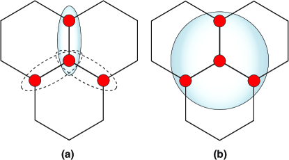
Figure 1: A nematic superconducting state in a lattice with three-fold or six-fold rotational symmetry (here, a honeycomb lattice is shown) is described by a two-component order parameter $\left(\Delta_{1},\,\Delta_{2}\right)=\Delta_{0}\left(\cos\theta,\,\sin\theta\right)$, represented here by bound states of electron pairs (red dots). The ellipses represent, schematically, different orientations $\theta$. Two competing vestigial phases are supported: (a) a Potts-nematic phase and (b) a charge-$4e$ phase. In (a), the angle $\theta$ associated with the nematic director is fixed, breaking the three-fold rotational symmetry. In (b), the three-fold rotational symmetry is preserved and a coherent state of bound states of four electrons emerge. In both (a) and (b), $\left\langle\Delta_{i}\right\rangle=0$, i.e. charge-$2e$ superconducting order is absent.

Such an intermediate phase is called a vestigial phase (Nie et al., 2014; Fradkin et al., 2015; Fernandes et al., 2019), as it breaks a subset of the symmetries broken in the primary PDW state. The main drawback of this interesting idea is the fact that the occurrence of PDW states in actual materials seems to be rather rare (Agterberg et al., 2020). Even from a purely theoretical standpoint, challenges remain in finding microscopic models that give a PDW ground state rather than a uniform superconducting ground state. For these reasons, it is desirable to search for other systems that may host vestigial charge-$4e$ superconductivity.

In this paper, we show that nematic superconductors in hexagonal and trigonal lattices offer a promising alternative. A nematic superconductor breaks both the gauge symmetry associated with the phase of the gap function and the three-fold/six-fold rotational symmetry of the lattice. Importantly, nematic superconductivity has been experimentally observed in doped Bi₂Se₃ (Matano et al., 2016; Yonezawa et al., 2017) and in twisted bilayer graphene (Cao et al., 2020), two systems whose lattices have three-fold rotational symmetry. Superconducting properties that do not respect the three-fold lattice symmetry were also observed in few-layer NbSe₂, although it is unclear whether this is a consequence of a nematic pairing state (Hamill et al., 2020; Cho et al., 2020a). Unless finite tuning is invoked (Chichinadze et al., 2020; Wang et al., 2020), nematic superconductivity is realized in systems where the order parameter transforms as a multi-dimensional irreducible representation of the relevant point group $G$ (Fu, 2014; Venderbos et al., 2016a; Venderbos and Fernandes, 2018; Su and Lin, 2018; Kozii et al., 2019; Cao et al., 2020). Typical examples are two-dimensional representations $\left(\Delta_{1},\,\Delta_{2}\right)$ where $\Delta_{1}$ and $\Delta_{2}$ correspond to $p_{x}$-wave/$p_{y}$-wave gaps or $d_{x^{2}-y^{2}}$-wave/$d_{xy}$-wave gaps. Interestingly, it has been shown that a secondary composite order parameter $\bm{\Phi}=\left(\left|\Delta_{1}\right|^{2}-\left|\Delta_{2}\right|^{2},-\Delta_{1}\Delta_{2}^{*}-\Delta_{1}^{*}\Delta_{2}\right)$, corresponding to Potts-nematic order, can onset even above the superconducting transition temperature $T_{c}$ (Hecker and Schmalian, 2018; Venderbos and Fernandes, 2018).

In this paper, we show that the very same mechanism that favors a vestigial nematic phase also promotes a vestigial charge-$4e$ phase characterized by a non-zero composite order parameter $\psi=\Delta_{1}^{2}+\Delta_{2}^{2}$ , but $\left\langle\Delta_{i}\right\rangle=0$ (see Fig. 1). In particular, we find that the effective Ginzburg-Landau theory obtained after integrating out the normal-state superconducting fluctuations has the same form for both the nematic order parameter $\bm{\Phi}$ and the charge-$4e$ order parameter $\psi$. We show that this is a robust result stemming from the existence of a linear transformation, called a perfect shuffle permutation, that relates $\bm{\Phi}$ and $\psi$ in the four-dimensional space spanned by $\Delta_{1}$ and $\Delta_{2}$. Such a transformation effectively permutes quantities in the “gauge sector” and in the “crystalline sector” of the group $\mathrm{U}(1)\otimes G$ that defines the symmetry properties of the system.

This result implies that there are actually two competing vestigial phases that can onset before long-range superconductivity sets in: nematic order, as studied previously (Hecker and Schmalian, 2018; Venderbos and Fernandes, 2018), and charge-$4e$ superconductivity. While higher-order terms in the superconducting free-energy generally favor the former, we show that the coupling to random strain can fundamentally alter the balance between them. This is because random strain acts as a random-field to $\bm{\Phi}$, but as a random-mass to $\psi$. Consequently, random strain, intrinsically present in actual materials, is expected to suppress Potts-nematic order much more strongly than charge-$4e$ order. We thus conclude that the most promising candidates to realize vestigial charge-$4e$ superconductivity are relatively inhomogeneous nematic superconductors with strong superconducting fluctuations, as expected for instance in quasi-2D systems. This analysis thus suggests that twisted bilayer graphene (Cao et al., 2018a, b; Yankowitz et al., 2019; Lu et al., 2019; Sharpe et al., 2019; Kerelsky et al., 2019; Jiang et al., 2019; Choi et al., 2019; Xie et al., 2019) offers a potentially viable platform to realize this elusive state of matter.

Vestigial nematicity: the standard scenario. We consider a nematic superconductor in a lattice with three-fold or six-fold rotational symmetry, described by a two-component order parameter $\left(\Delta_{1},\,\Delta_{2}\right)$. For concreteness, hereafter we will focus on the case where the point group of the lattice is $D_{6}$, and $\bm{\Delta}\equiv\left(\Delta_{1},\,\Delta_{2}\right)^{\dagger}$ transforms as the $E_{2}$ irreducible representation (irrep), corresponding to $\left(d_{x^{2}-y^{2}},\,d_{xy}\right)$-wave gaps. Importantly, our results are general and hold as long as $\bm{\Delta}$ transforms as one of the two-dimensional $E$-like irreps of the corresponding point group $D_{6}$, $D_{3}$, $C_{3v}$, etc. The Ginzburg-Landau superconducting action expanded to fourth order in $\bm{\Delta}$ is given by (Sigrist and Ueda, 1991; Hecker and Schmalian, 2018; Venderbos and Fernandes, 2018; Chichinadze et al., 2020):

$$S\left[\bm{\Delta}\right] =\int_{q}\Delta_{i,q}^{*}\chi_{ij}^{-1}\left(q\right)\Delta_{j,q}+\frac{u_{0}}{2}\int_{r}\left(\left|\Delta_{1}\right|^{2}+\left|\Delta_{2}\right|^{2}\right)^{2}$$

$$+\frac{\gamma}{2}\int_{r}\left|\Delta_{1}\Delta_{2}^{*}-\Delta_{1}^{*}\Delta_{2}\right|^{2}$$ (1)

Here, $\chi_{ij}^{-1}\left(q\right)$ is the inverse superconducting susceptibility in Fourier space, whereas $u_{0}>0$ and $\gamma$ are Ginzburg-Landau parameters. Furthermore, $q=\left(\mathbf{q},\omega_{n}\right)$ and $r=\left(\mathbf{r},\tau\right)$, where $\mathbf{q}$ is the momentum, $\omega_{n}$ is the bosonic Matsubara frequency, $\mathbf{r}$ is the position, and $\tau$ is the imaginary time. Note that $S$ has an enlarged continuous rotational symmetry $\Delta_{1}\pm i\Delta_{2}\rightarrow e^{\pm i\theta}(\Delta_{1}\pm i\Delta_{2})$. This emergent continuous rotational symmetry is reduced to discrete ones only when higher-order terms are included, as we discuss later.

The superconducting ground state depends on $\gamma$: if $\gamma<0$, the action is minimized by $\bm{\Delta}=\Delta_{0}\left(1,\,\pm i\right)^{\dagger}$, corresponding to a time-reversal symmetry-breaking (TRSB) superconductor that preserves the six-fold rotational symmetry of the lattice. On the other hand, for $\gamma>0$, the ground state is given by $\bm{\Delta}=\Delta_{0}\left(\cos\theta,\,\sin\theta\right)^{\dagger}$, with arbitrary $\theta$. Such a pairing state is called nematic, as it preserves time-reversal symmetry but lowers the six-fold rotational symmetry of the lattice to two-fold. It is convenient to construct the real-valued composite order parameters $\zeta\equiv\bm{\Delta}^{\dagger}\sigma^{y}\bm{\Delta}$ and $\bm{\Phi}\equiv\left(\bm{\Delta}^{\dagger}\sigma^{z}\bm{\Delta},\,-\bm{\Delta}^{\dagger}\sigma^{x}\bm{\Delta}\right)$, where $\sigma^{\mu}$ is a Pauli matrix that acts on the two-dimensional subspace spanned by $\bm{\Delta}$ (Hecker and Schmalian, 2018; Venderbos and Fernandes, 2018; Fernandes et al., 2019). While $\zeta$ transforms as the $A_{2}$ irrep of $D_{6}$, and is thus related to TRSB, $\bm{\Phi}$ transforms as the $E_{2}$ irrep, being related to six-fold rotational symmetry breaking. Clearly, if the ground state is $\bm{\Delta}=\Delta_{0}\left(1,\,\pm i\right)^{\dagger}$, $\zeta\neq 0$ but $\bm{\Phi}=0$. On the other hand, if $\bm{\Delta}=\Delta_{0}\left(\cos\theta,\,\sin\theta\right)^{\dagger}$, $\zeta=0$ while $\bm{\Phi}\neq 0$. The sign of $\gamma$ is ultimately determined by microscopic considerations. While weak-coupling calculations tend to favor $\gamma<0$ (Nandkishore et al., 2012; Kozii et al., 2019; Chichinadze et al., 2020), the presence of strong spin-orbit coupling or of density-wave/nematic fluctuations can tip the balance in favor of the nematic superconducting state (Fu, 2014; Venderbos et al., 2016a; Kozii et al., 2019; Fernandes and Millis, 2013). Hereafter, we will assume one of these microscopic mechanisms as the source of $\gamma>0$.

The nematic superconducting state supports a vestigial nematic phase, i.e. a phase in which the composite nematic order parameter is non-zero, $\left\langle\bm{\Phi}\right\rangle\neq 0$, but superconducting order is absent, $\left\langle\bm{\Delta}\right\rangle=0$ (see Fig. 1(a)). To see this, we follow the procedure outlined in Ref. (Fernandes et al., 2019) and first note that the quartic terms in Eq. (1) can be rewritten in terms of the TRSB bilinear $\zeta=\bm{\Delta}^{\dagger}\sigma^{y}\bm{\Delta}$ and the trivial bilinear $\lambda\equiv\bm{\Delta}^{\dagger}\sigma^{0}\bm{\Delta}$ as $S^{(4)}=\frac{u_{0}}{2}\int_{r}\lambda^{2}+\frac{\gamma}{2}\int_{r}\zeta^{2}$. Here, $\sigma^{0}$ is the identity matrix. Now, the Fierz identity $\sum_{\mu}\sigma_{ij}^{\mu}\sigma_{kl}^{\mu}=2\delta_{il}\delta_{jk}-\sigma_{ij}^{0}\sigma_{kl}^{0}$ implies a relationship between the bilinears, $\zeta^{2}=\lambda^{2}-\Phi^{2}$. As a result, the quartic term can be rewritten as $S^{(4)}=\frac{u}{2}\int_{r}\lambda^{2}-\frac{\gamma}{2}\int_{r}\Phi^{2}$, where $u\equiv u_{0}+\gamma$ and, as defined above, $\bm{\Phi}=\left(\Phi_{1},\Phi_{2}\right)=\left(\bm{\Delta}^{\dagger}\sigma^{z}\bm{\Delta},\,-\bm{\Delta}^{\dagger}\sigma^{x}\bm{\Delta}\right)$ is the nematic bilinear. Since $\gamma>0$ by assumption, we can perform Hubbard-Stratonovich transformations to decouple the quartic terms and obtain:

$$S \left[\bm{\Delta},\lambda,\bm{\Phi}\right]=\int_{r}\frac{\Phi^{2}}{2\gamma}-\int_{r}\frac{\lambda^{2}}{2u}$$

$$+\int_{q}\Delta_{i,q}^{*}\left[\chi_{ij}^{-1}\left(q\right)+\lambda\sigma_{ij}^{0}-\Phi_{1}\sigma_{ij}^{z}+\Phi_{2}\sigma_{ij}^{x}\right]\Delta_{j,q}$$ (2)

Note that $\bm{\Phi}$ and $\lambda$ have been promoted to independent auxiliary fields. Because the action is quadratic in $\Delta_{i}$, the superconducting fluctuations can be exactly integrated out in the normal state, yielding an effective action for $\bm{\Phi}$ and $\lambda$ . Since $\lambda$ does not break any symmetries, it is always non-zero and simply renormalizes the static superconducting susceptibility. On the other hand, $\bm{\Phi}$ is only non-zero below an onset temperature. A large-$N$ calculation (Fernandes et al., 2012), as performed in Ref. (Hecker and Schmalian, 2018), indicates that $\left\langle\bm{\Phi}\right\rangle\neq 0$ already above $T_{c}$, implying that vestigial nematic order precedes the onset of superconductivity (see also the Supplementary Material, SM). Interestingly, a vestigial nematic phase has been recently observed in doped Bi₂Se₃ (Sun et al., 2019; Cho et al., 2020b).

Competition between nematicity and charge-$4e$ superconductivity. We now show that there is a hidden symmetry between the two-component real-valued nematic order parameter $\bm{\Phi}$ and the complex bilinear $\psi\equiv\Delta_{1}^{2}+\Delta_{2}^{2}$. The latter breaks the U(1) gauge symmetry and is precisely the charge-$4e$ order parameter (see Fig. 1(b)). Importantly, $\psi\neq 0$ ($\psi=0$) inside the nematic (TRSB) superconducting state.

To see the unexpected connection between these two order parameters, we need to consider, besides the real bilinears discussed above, complex bilinears formed out of the primary order parameter $\bm{\Delta}$, since the latter transforms as the irrep $\Gamma=\mathrm{e}^{im\theta}\otimes E_{2}$ of the group $\mathrm{U}(1)\otimes D_{6}$. Writing the order parameter explicitly as a four-dimensional vector $\bm{\eta}\equiv\left(\Delta^{\prime}_{1},\,\Delta^{\prime\prime}_{1},\Delta^{\prime}_{2},\,\Delta^{\prime\prime}_{2}\right)^{T}$, where the prime (double prime) denotes the real (imaginary) part, the bilinears are generally given by $\bm{\eta}^{T}\left(\sigma^{\mu}\otimes\sigma^{m}\right)\bm{\eta}$. Here, the first Pauli matrix (with Greek superscript) in the Kronecker product $\sigma^{\mu}\otimes\sigma^{m}$ refers to the subspace associated with the two-dimensional irreducible representation $E_{2}$ of the point group $D_{6}$ (dubbed the crystalline sector), whereas the second Pauli matrix (with Latin superscript) refers to the subspace associated with the U(1) group (dubbed the gauge sector). In this notation, the components of the nematic bilinear become:

$$\Phi_{1} =\bm{\eta}^{T}\left(\sigma^{z}\otimes\sigma^{0}\right)\bm{\eta}$$

$$\Phi_{2} =-\bm{\eta}^{T}\left(\sigma^{x}\otimes\sigma^{0}\right)\bm{\eta}$$ (3)

The other real bilinears are given by $\zeta=\bm{\eta}^{T}\left(\sigma^{y}\otimes\sigma^{y}\right)\bm{\eta}$ and $\lambda=\bm{\eta}^{T}\left(\sigma^{0}\otimes\sigma^{0}\right)\bm{\eta}$. The charge-$4e$ bilinear $\psi\equiv\psi^{\prime}+i\psi^{\prime\prime}$, on the other hand, is:

$$\psi^{\prime} =\bm{\eta}^{T}\left(\sigma^{0}\otimes\sigma^{z}\right)\bm{\eta}$$

$$\psi^{\prime\prime} =\bm{\eta}^{T}\left(\sigma^{0}\otimes\sigma^{x}\right)\bm{\eta}$$ (4)

The key point is that, although the Kronecker product $\left(M\otimes N\right)$ is non-commutative, in the case where $M$ and $N$ are square matrices it satisfies the property $\left(M\otimes N\right)=\tilde{P}^{T}\left(N\otimes M\right)\tilde{P}$, where $\tilde{P}$ is the so-called perfect shuffle permutation matrix (Davio, 1981). Here, due to the minus sign in the second equation of (3), a slightly modified $2\times 2$ matrix $P$ is needed:

$$P=\left(\begin{array}[]{cccc}1&0&0&0\\ 0&0&-1&0\\ 0&-1&0&0\\ 0&0&0&1\end{array}\right)$$ (5)

Physically, $P$ permutes quantities from the crystalline and the gauge sectors of the four-dimensional space spanned by $\bm{\eta}$. Note that $P$ is an orthogonal matrix, $P^{-1}=P^{T}=P$. As a result, upon performing the unitary transformation $\tilde{\bm{\eta}}=P\bm{\eta}$, we see that while the bilinears $\zeta$ and $\lambda$ remain invariant, $\left(\Phi_{1},\Phi_{2}\right)\rightarrow\left(\psi^{\prime},\psi^{\prime\prime}\right)$, i.e. the nematic bilinear is mapped onto the charge-$4e$ bilinear. Consequently, provided that the susceptibility in the quadratic term of Eq. (1) is invariant under the linear transformation (S35), the effective action in the normal state has the same functional form with respect to either $\Phi^{2}$ or $\left|\psi\right|^{2}$. This is the case if we consider the standard susceptibility expression $\chi_{ij}^{-1}\left(q\right)=\left(r_{0}+q^{2}\right)\delta_{ij}$, where $r_{0}\propto T-T_{c,0}$ is a tuning parameter and $T_{c,0}$ is the bare superconducting transition temperature (see the SM).

This is the main result of our paper: for the Ginzburg-Landau action in Eq. (1), which describes a nematic superconducting ground state in a lattice with three-fold or six-fold rotational symmetry, an instability towards a vestigial nematic state at $T_{\mathrm{nem}}$ implies an instability towards a vestigial charge-$4e$ state at the same temperature $T_{4e}=T_{\mathrm{nem}}$. This degeneracy between nematicity and charge-$4e$ superconductivity is rooted on the invariance of the action upon a perfect shuffle that permutes elements from the crystalline and the gauge sectors.

Selecting nematic or charge-$4e$ order. While the competition between vestigial charge-$4e$ and nematic orders is robust, their degeneracy is lifted by additional terms in the action not considered in the analysis above. For instance, additional symmetry-allowed terms in the susceptibility $\chi(q)$ can favor either the charge-$4e$ state, in the case of a hexagonal lattice, or the nematic state, in the case of a trigonal lattice (see SM). While here we focus on classical phase transitions, where the dynamics of $\chi(q)$ is not important, the situation changes in the case of quantum phase transitions, as the couplings between the bosonic fields $\bm{\Phi}$ and $\psi$ and the electrons are expected to generate different types of bosonic dynamics.

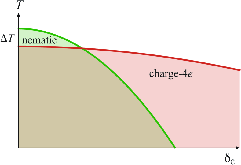
Figure 2: Schematic phase diagram of the vestigial nematic (transition temperature $T_{\mathrm{nem}}$, green) and vestigial charge-$4e$ ($T_{4e}$, red) phases. Here, $\delta_{\varepsilon}$ represents the strength of strain inhomogeneity. Because random strain couples as a random-field to the nematic order parameter but as a random-mass to the charge-$4e$ order parameter, the former is expected to be suppressed much more strongly than the latter. In the clean system, $\Delta T\equiv T_{\mathrm{nem}}-T_{4e}$ is positive because of the sixth-order term in Eq. (6) that restricts the nematic director to three directions (3-state Potts nematicity) and lifts the emergent degeneracy between the two vestigial ordered phases. Note that, as temperature is lowered, a superconducting transition is expected (not shown here). Whether charge-$4e$ and nematic orders can coexist in the overlapping region of the phase diagram remains to be studied.

More importantly, because the nematic order parameter $\bm{\Phi}$ is real and transforms as the $E_{2}$ irrep of $D_{6}$, there is a symmetry-allowed cubic term in the nematic action proportional to $\left(\Phi_{+}^{3}+\Phi_{-}^{3}\right)$, where $\Phi_{\pm}=\Phi_{1}\pm i\Phi_{2}$ (Fu, 2014; Hecker and Schmalian, 2018; Venderbos and Fernandes, 2018; Xu et al., 2020; Fernandes and Venderbos, 2020). This term is related to a particular sixth-order term in the superconducting action (1) (Sigrist and Ueda, 1991):

$$S^{(6)}\left[\bm{\Delta}\right]\propto\int_{r}\left(\Delta_{1}+i\Delta_{2}\right)^{3}\left(\Delta_{1}^{*}+i\Delta_{2}^{*}\right)^{3}+\mathrm{h.c.}$$ (6)

In contrast, because $\psi$ is complex and transforms as the $A_{1}$ irrep of $D_{6}$, such a cubic term is not allowed in the charge-$4e$ action. This cubic term not only favors the nematic order over the charge-$4e$ order, but it also lowers the symmetry of the nematic order parameter from U$(1)$ to 3-state Potts (Hecker and Schmalian, 2018; Venderbos and Fernandes, 2018; Xu et al., 2020; Jin et al., 2019). At first sight, this seems to suggest that it would be challenging to find a vestigial charge-$4e$ instability occurring before the onset of vestigial nematic order. While it is possible that charge-$4e$ order could coexist with nematic order and onset at a temperature between $T_{\mathrm{nem}}$ and $T_{c}$ (the renormalized superconducting transition temperature), this seems to be a rather contrived scenario. However, there is an important ingredient missing in the analysis: the coupling to lattice degrees of freedom. This is particularly important for nematic order, as it is known to trigger lattice distortions (Fernandes and Venderbos, 2020).

We thus introduce the strain tensor $\varepsilon_{ij}=\frac{1}{2}\left(\partial_{i}u_{j}+\partial_{j}u_{i}\right)$, with $\mathbf{u}$ denoting the lattice displacement vector. Decomposing it in the irreps of the $D_{6}$ group, there are two relevant modes: the longitudinal mode, which transforms as $A_{1}$, $\varepsilon_{A}\equiv\varepsilon_{xx}+\varepsilon_{yy}+\varepsilon_{zz}$, and the shear mode, which transforms as $E_{2}$, $\bm{\varepsilon}_{E}\equiv\left(\varepsilon_{xx}-\varepsilon_{yy},\,-2\varepsilon_{xy}\right)$. The leading-order couplings to the nematic and charge-$4e$ orders are given, respectively, by the linear coupling $\bm{\varepsilon}_{E}\cdot\bm{\Phi}$ and by the quadratic coupling $\varepsilon_{A}\left|\psi\right|^{2}$. While strain can be externally applied, it is intrinsically present in materials as random strain caused by defects arising in the crystal growth or device fabrication. The key point is that random strain acts as a random-field to the Potts-nematic order parameter, but as a random-mass (also called random-$T_{c}$) to the charge-$4e$ order parameter.

This distinction is very important, as random-field disorder is known to be much more detrimental to long-order range order than random-mass disorder. In the specific case of the 3-state Potts model, random-field is believed to completely kill the Potts transition in two dimensions, and to suppress it in three dimensions (Blankschtein et al., 1984; Eichhorn and Binder, 1996; Kumar et al., 2018). Thus, one generally expects random strain to tilt the balance between the competing vestigial charge-$4e$ and nematic orders in favor of the former. The resulting schematic phase diagram is shown in Fig. 2.

The condition $T_{4e}>T_{\mathrm{nem}}$ is not enough to ensure a vestigial charge-$4e$ phase, as one needs to show also that the renormalized superconducting transition temperature $T_{c}$ inside the charge-$4e$ state is split from $T_{4e}$ (Fernandes et al., 2019). A large-$N$ analysis indicates that, for sufficiently anisotropic quasi-two-dimensional systems, $T_{4e}$ and $T_{c}$ are indeed split (Fernandes et al., 2012; Hecker and Schmalian, 2018). In this case, while the transition at $T_{4e}$ is XY-like, the transition at $T_{c}$ is Ising-like due to the coupling $\psi^{*}\left(\Delta_{1}^{2}+\Delta_{2}^{2}\right)$ between the charge-$4e$ and the superconducting order parameters (Jiang et al., 2017).

Conclusions. In this paper, we showed that a nematic superconductor in lattices with three-fold or six-fold rotational symmetry supports competing nematic and charge-$4e$ vestigial orders. Such a competition is rooted on a perfect shuffle permutation that transforms one order parameter onto the other in the four-dimensional space spanned by the multi-component superconducting order parameter. We showed that random strain provides the most promising tuning knob to favor charge-$4e$ superconductivity over nematic order, due to the fact that it acts as a random-field disorder to the latter, but as a random-mass disorder to the latter. These results establish a new class of systems – nematic superconductors – in which charge-$4e$ order may be realized.

Nematic superconductivity has been now observed in doped Bi₂Se₃ and in twisted bilayer graphene (Matano et al., 2016; Yonezawa et al., 2017; Cao et al., 2020). Based on our results, the most favorable conditions for the observation of charge-$4e$ superconductivity are systems where superconducting fluctuations are strong (e.g. quasi-2D superconductors) and where random-strain is present (e.g. inhomogeneous superconductors). Twisted bilayer graphene seems to satisfy both conditions, given the ubiquitous twist angle inhomogeneity (Uri et al., 2020; Wilson et al., 2020; Padhi et al., 2020; Tschirhart et al., 2020), and is thus a promising place to look for this elusive state of matter. Note that the mechanism proposed here, which relies on an exact discrete symmetry in Ginzburg-Landau theory for multi-component superconductors in general, is different from a recent proposal for charge-$4e$ superconductivity based on an approximate SU(4) symmetry of twisted bilayer graphene (Khalaf et al., 2020).

Supplementary material for “Charge-$4e$ superconductivity from multi-component nematic pairing: Application to twisted bilayer graphene”

Derivation of the effective action within large-$N$

Here we derive the explicit form of the effective nematic/charge-$4e$ action by performing a large-$N$ calculation, extending the general procedure outlined in Refs. (Fernandes et al., 2012; Hecker and Schmalian, 2018; Fernandes et al., 2019). For a system with $D_{6}$ point group symmetry, the most general form of the quadratic part of the superconducting action is given by (Sigrist and Ueda, 1991; Venderbos et al., 2016b):

$$S^{(2)}\left[\bm{\Delta}\right] =\int_{q}\left(r_{0}+q_{\parallel}^{2}+\upsilon q_{z}^{2}\right)\left(\left|\Delta_{1,q}\right|^{2}+\left|\Delta_{2,q}\right|^{2}\right)$$

$$+\kappa\int_{q}\left[\left(q_{x}^{2}-q_{y}^{2}\right)\left(\left|\Delta_{1,q}\right|^{2}-\left|\Delta_{2,q}\right|^{2}\right)\right.$$

$$\left.+2q_{x}q_{y}\left(\Delta_{1,q}\Delta_{2,q}^{*}+\Delta_{1,q}^{*}\Delta_{2,q}\right)\right]$$ (S1)

where $\mathbf{q}_{\parallel}\equiv\left(q_{x},\,q_{y}\right)$ and $\upsilon>0$, $\left|\kappa\right|<1$ are constants. In terms of the vector $\bm{\eta}\equiv\left(\Delta^{\prime}_{1},\,\Delta^{\prime\prime}_{1},\Delta^{\prime}_{2},\,\Delta^{\prime\prime}_{2}\right)^{T}$, it can be rewritten as:

$$S^{(2)}\left[\bm{\eta}\right]=\int_{q}\bm{\eta}_{q}^{T}\hat{\chi}_{0}^{-1}(q)\bm{\eta}_{-q}$$ (S2)

with:

$$\hat{\chi}_{0}^{-1}\left(q\right) =\left(r_{0}+q_{\parallel}^{2}+\upsilon q_{z}^{2}\right)\hat{\mathbb{I}}$$

$$+\kappa q_{\parallel}^{2}\left(\cos 2\theta\,\hat{A}_{1}-\sin 2\theta\,\hat{A}_{2}\right)$$ (S3)

Here, $\theta\equiv\arctan\left(\frac{q_{y}}{q_{x}}\right)$, the hat denotes a $4\times 4$ matrix and $\hat{\mathbb{I}}\equiv\sigma^{0}\otimes\sigma^{0}$, $\hat{A}_{1}\equiv\sigma^{z}\otimes\sigma^{0}$, $\hat{A}_{2}\equiv-\sigma^{x}\otimes\sigma^{0}$. Explicitly:

$$\hat{A}_{1} =\left(\begin{array}[]{cccc}1&0&0&0\\ 0&1&0&0\\ 0&0&-1&0\\ 0&0&0&-1\end{array}\right)$$ (S8)

$$\hat{A}_{2} =\left(\begin{array}[]{cccc}0&0&-1&0\\ 0&0&0&-1\\ -1&0&0&0\\ 0&-1&0&0\end{array}\right)$$ (S13)

We now move on to the quartic terms. The first one is given by:

$$S_{1}^{(4)}\left[\bm{\Delta}\right] =\frac{u}{2}\int_{r}\left(\left|\Delta_{1}\right|^{2}+\left|\Delta_{2}\right|^{2}\right)^{2}=\frac{u}{2}\int_{r}\left(\bm{\eta}^{T}\hat{\mathbb{I}}\bm{\eta}\right)^{2}$$ (S14)

Performing a Hubbard-Stratonovich transformation, we introduce the auxiliary field $\lambda$ and obtain:

$$S_{1}^{(4)}\left[\bm{\eta},\lambda\right]=-\int_{r}\frac{\lambda^{2}}{2u}+\int_{r}\lambda\left(\bm{\eta}^{T}\hat{\mathbb{I}}\bm{\eta}\right)$$ (S15)

As for the second quartic term,

$$S_{2}^{(4)}\left[\bm{\Delta}\right] =-\frac{\gamma}{2}\int_{r}\left[\left(\left|\Delta_{1}\right|^{2}-\left|\Delta_{2}\right|^{2}\right)^{2}\right.$$

$$\left.+\left(\Delta_{1}\Delta_{2}^{*}+\Delta_{1}^{*}\Delta_{2}\right)^{2}\right]$$ (S16)

there are two different ways to decouple it in terms of auxiliary fields. In the first case, we introduce the nematic field:

$$S_{2}^{(4)}\left[\bm{\eta},\bm{\Phi}\right]=\int_{r}\frac{\Phi^{2}}{2\gamma}-\int_{r}\left[\Phi_{1}\left(\bm{\eta}^{T}\hat{A}_{1}\bm{\eta}\right)+\Phi_{2}\left(\bm{\eta}^{T}\hat{A}_{2}\bm{\eta}\right)\right]$$ (S17)

An alternative way to decouple it is by using the identity:

$$\left[\left(\left|\Delta_{1}\right|^{2}-\left|\Delta_{2}\right|^{2}\right)^{2}+\left(\Delta_{1}\Delta_{2}^{*}+\Delta_{1}^{*}\Delta_{2}\right)^{2}\right] =$$

$$\left[\Delta_{1}^{2}+\Delta_{2}^{2}\right]\left[\left(\Delta_{1}^{*}\right)^{2}+\left(\Delta_{2}^{*}\right)^{2}\right]$$ (S18)

We then introduce the charge-$4e$ auxiliary field $\psi$ and obtain:

$$S_{2}^{(4)}\left[\bm{\eta},\psi\right]=\int_{r}\frac{\left|\psi\right|^{2}}{2\gamma}-\int_{r}\left[\psi^{\prime}\left(\bm{\eta}^{T}\hat{B}_{1}\bm{\eta}\right)+\psi^{\prime\prime}\left(\bm{\eta}^{T}\hat{B}_{2}\bm{\eta}\right)\right]$$ (S19)

where we defined $\hat{B}_{1}\equiv\sigma^{0}\otimes\sigma^{z}$ and $\hat{B}_{2}\equiv\sigma^{0}\otimes\sigma^{x}$, i.e.

$$\hat{B}_{1} =\left(\begin{array}[]{cccc}1&0&0&0\\ 0&-1&0&0\\ 0&0&1&0\\ 0&0&0&-1\end{array}\right)$$ (S24)

$$\hat{B}_{2} =\left(\begin{array}[]{cccc}0&1&0&0\\ 1&0&0&0\\ 0&0&0&1\\ 0&0&1&0\end{array}\right)$$ (S29)

The action can thus be written as:

$$S_{\mathrm{nem}}\left[\bm{\eta},\lambda,\bm{\Phi}\right] =\int_{q}\bm{\eta}_{q}^{T}\left[\hat{\chi}^{-1}(q)-\sum_{i}\Phi_{i}\hat{A}_{i}\right]\bm{\eta}_{-q}$$

$$+\int_{r}\frac{\Phi^{2}}{2\gamma}-\int_{r}\frac{\lambda^{2}}{2u}$$ (S30)

or, equivalently,

$$S_{4e}\left[\bm{\eta},\lambda,\psi\right] =\int_{q}\bm{\eta}_{q}^{T}\left[\hat{\chi}^{-1}(q)-\sum_{i}\psi_{i}\hat{B}_{i}\right]\bm{\eta}_{-q}$$

$$+\int_{r}\frac{\left|\psi\right|^{2}}{2\gamma}-\int_{r}\frac{\lambda^{2}}{2u}$$ (S31)

Here, to simplify the notation, we introduced $\psi_{1}=\psi^{\prime}$ and $\psi_{2}=\psi^{\prime\prime}$. Moreover, we defined:

$$\hat{\chi}^{-1}(q)=\hat{\chi}_{0}^{-1}(q)+\lambda\hat{\mathbb{I}}$$ (S32)

which corresponds to shifting the superconducting mass term to $r=r_{0}+\lambda$. Integrating out the superconducting fluctuations:

$$\int D\bm{\eta}\exp\left\{-\int_{q}\bm{\eta}_{q}^{T}\left[\hat{\chi}^{-1}(q)-\hat{V}\right]\bm{\eta}_{-q}\right\} =$$

$$\mathcal{N}\exp\left\{-\frac{1}{2}\int_{q}\mathrm{Tr}\ln\left[\hat{\chi}^{-1}\left(q\right)-\hat{V}\right]\right\}$$

gives the effective actions:

$$S_{\mathrm{nem}}^{(\mathrm{eff})}\left[\lambda,\bm{\Phi}\right] =-\sum_{n=1}^{\infty}\frac{1}{2n}\int_{q}\mathrm{Tr}\left[\hat{\chi}\left(q\right)\hat{V}_{\mathrm{nem}}\right]^{n}+\int_{r}\frac{\Phi^{2}}{2\gamma}-\int_{r}\frac{\lambda^{2}}{2u}$$ (S33)

$$S_{4e}^{(\mathrm{eff})}\left[\lambda,\psi\right] =-\sum_{n=1}^{\infty}\frac{1}{2n}\int_{q}\mathrm{Tr}\left[\hat{\chi}\left(q\right)\hat{V}_{4e}\right]^{n}+\int_{r}\frac{\left|\psi\right|^{2}}{2\gamma}-\int_{r}\frac{\lambda^{2}}{2u}$$ (S34)

where $\hat{V}_{\mathrm{nem}}=\sum_{i}\Phi_{i}\hat{A}_{i}$ and $\hat{V}_{4e}=\sum_{i}\psi_{i}\hat{B}_{i}$. Now, to relate $\hat{A}_{i}$ and $\hat{B}_{i}$, we note the identity $\left(M\otimes N\right)=\tilde{P}^{T}\left(N\otimes M\right)\tilde{P}$ for $2\times 2$ matrices $M,\,N$, where $\tilde{P}$ is the perfect shuffle permutation matrix (Davio, 1981):

$$\tilde{P}=\left(\begin{array}[]{cccc}1&0&0&0\\ 0&0&1&0\\ 0&1&0&0\\ 0&0&0&1\end{array}\right)$$

which is orthogonal. In our case, due to the extra minus sign in Eq. (S13), we need a slightly modified orthogonal matrix:

$$P=\left(\begin{array}[]{cccc}1&0&0&0\\ 0&0&-1&0\\ 0&-1&0&0\\ 0&0&0&1\end{array}\right)$$ (S35)

which then gives $\hat{B}_{i}=\hat{P}^{T}\hat{A}_{i}\hat{P}$ as defined in Eqs. (S8), (S13), (S24), and (S29). Thus, we obtain:

$$\mathrm{Tr}\left[\hat{\chi}\left(q\right)\hat{V}_{\mathrm{nem}}\right]^{n}=\mathrm{Tr}\left[\hat{\tilde{\chi}}\left(q\right)\hat{V}_{4e}\right]^{n}$$ (S36)

upon exchanging $\psi_{i}\longleftrightarrow\Phi_{i}$. Here, $\hat{\tilde{\chi}}\equiv\hat{P}^{T}\hat{\chi}\hat{P}$. Thus, as long as $\kappa=0$ in Eq. (S3), we have $\hat{\tilde{\chi}}\equiv\hat{\chi}$, implying that the two actions – nematic and charge-$4e$ – are identical.

We now proceed to investigate the impact of $\kappa\neq 0$. For simplicity, we focus on the two-dimensional case, setting $\upsilon=0$ in Eq. (S3). We also consider classical finite-temperature phase transitions. Performing the traces and integrals in Eqs. (S33)-(S34) and assuming uniform order parameters, we obtain the free-energy densities (the Ginzburg-Landau constants $\gamma$ and $u$ are rescaled by a factor of temperature):

$$F_{\mathrm{nem}}^{(\mathrm{eff})}\left[r,\bm{\Phi}\right]=\frac{\Phi^{2}}{2}\left\{\frac{1}{\gamma}-\int_{0}^{\infty}\frac{qdq}{\pi}\,\frac{\left(q^{2}+r\right)^{2}}{\left[\kappa^{2}q^{4}-\left(q^{2}+r\right)^{2}\right]^{2}}\right\}$$

$$-\frac{\Phi^{4}}{4}\int_{0}^{\infty}\frac{qdq}{\pi}\,\frac{\left(q^{2}+r\right)^{2}\left[\left(q^{2}+r\right)^{2}+2\kappa^{2}q^{4}\right]}{\left[\kappa^{2}q^{4}-\left(q^{2}+r\right)^{2}\right]^{4}}$$

$$-\frac{(r-r_{0})^{2}}{2u}$$ (S37)

and:

$$F_{4e}^{(\mathrm{eff})}\left[r,\psi\right]=\frac{\left|\psi\right|^{2}}{2}\left\{\frac{1}{\gamma}-\int_{0}^{\infty}\frac{qdq}{\pi}\,\frac{\left[\left(q^{2}+r\right)^{2}+\kappa^{2}q^{4}\right]}{\left[\kappa^{2}q^{4}-\left(q^{2}+r\right)^{2}\right]^{2}}\right\}$$

$$-\frac{\left|\psi\right|^{4}}{4}\int_{0}^{\infty}\frac{qdq}{\pi}\,\frac{\left[\left(q^{2}+r\right)^{4}+6\kappa^{2}q^{4}\left(q^{2}+r\right)^{2}+\kappa^{4}q^{8}\right]}{\left[\kappa^{2}q^{4}-\left(q^{2}+r\right)^{2}\right]^{4}}$$

$$-\frac{(r-r_{0})^{2}}{2u}$$ (S38)

The mean-field transitions take place when the quadratic coefficients vanish. This gives the following critical values of $r$, $r_{\mathrm{nem}}=\gamma J_{\mathrm{nem}}$ and $r_{4e}=\gamma J_{4e}$, with:

$$J_{\mathrm{nem}} \equiv\int_{0}^{\infty}\frac{pdp}{\pi}\,\frac{\left(p^{2}+1\right)^{2}}{\left[\kappa^{2}p^{4}-\left(p^{2}+1\right)^{2}\right]^{2}}$$ (S39)

$$J_{4e} \equiv\int_{0}^{\infty}\frac{pdp}{\pi}\,\frac{\left[\left(p^{2}+1\right)^{2}+\kappa^{2}p^{4}\right]}{\left[\kappa^{2}p^{4}-\left(p^{2}+1\right)^{2}\right]^{2}}$$ (S40)

An explicit calculation gives:

$$J_{4e} =\frac{1}{2\pi\left(1-\kappa^{2}\right)}$$ (S41)

$$J_{\mathrm{nem}} =J_{4e}-\frac{1}{8\pi}\left[\frac{2}{1-\kappa^{2}}-\frac{1}{\kappa}\ln\left(\frac{1+\kappa}{1-\kappa}\right)\right]$$ (S42)

which implies that $J_{4e}>J_{\mathrm{nem}}$, i.e. $r_{4e}>r_{\mathrm{nem}}$. Now, $r$ is generally a decreasing function of temperature, since $r\propto\xi^{-2}\rightarrow 0$ at the bare superconducting transition temperature (here $\xi$ is the superconducting correlation length). Consequently, the $\kappa$ term in the action favors the charge-$4e$ instability over the nematic instability.

Note that this analysis is valid for the case of triangular or hexagonal lattices. For trigonal lattices, there is an additional allowed term in the susceptibility (S3) that depends on $q_{z}$ (Venderbos et al., 2016b). Such a term generates the cubic invariant $\Phi_{+}^{3}+\Phi_{-}^{3}$ in the nematic free energy (Hecker and Schmalian, 2018), with $\Phi_{\pm}=\Phi_{1}\pm\Phi_{2}$, which favors the nematic instability over the charge-$4e$ instability. Alternatively, this cubic term is expected to be generated from the sixth-order term of the superconducting action discussed in the main text.