Identifying First-order Lowpass Graph Signals using Perron Frobenius Theorem

Abstract

This paper is concerned with the blind identification of graph filters from graph signals. Our aim is to determine if the graph filter generating the graph signals is first-order lowpass without knowing the graph topology. Notice that lowpass graph filter is a common pre-requisite for applying graph signal processing tools for sampling, denoising, and graph learning. Our method is inspired by the Perron Frobenius theorem, which observes that for first-order lowpass graph filter, the top eigenvector of output covariance would be the only eigenvector with elements of the same sign. Utilizing this observation, we develop a simple detector that answers if a given data set is produced by a first-order lowpass graph filter. We analyze the effects of finite-sample, graph size, observation noise, strength of lowpass filter, on the detector’s performance. Numerical experiments on synthetic and real data support our findings.

Index Terms—  lowpass graph signals, graph learning, Perron Frobenius theorem

1 Introduction

A recent trend in data science is to develop tools for analyzing and inference from signals defined on graph, a.k.a. graph signals. Examples are financial and social networks data where graph structures can be leveraged to improve inference [1, 2]. These premises motivated researches on graph signal processing (GSP) [3, 4] which extends signal processing models to graph signals.

To study graph signals, an important concept of GSP is to model them as outputs from exciting a graph filter. The graph filter captures the social/physical process that generates the observations we collect. Examples are heat diffusion [5], dynamics of functional brain activities [6], equilibrium seeking in network games [7], etc.. Similar to its linear time invariant counterpart, the graph filters can be classified as lowpass, bandpass, highpass according to their frequency responses computed through the Graph Fourier transform [8]. Among others, lowpass graph filters and signals are important to many GSP tools, e.g., sampling, denoising, graph topology learning [9]. Importantly, a number of practical social/physical models can naturally lead to lowpass graph signals as studied in [9].

Although lowpass graph filters/signals are common, most prior works took the lowpass property as a default assumption without further verification. This paper takes a different approach, where we address the validity of the lowpass assumption for a given set of graph signals. Our approach is data-driven, and we aim to provide certificates on whether certain GSP tools are applicable to a dataset whose social/physical models are unknown, as well as determining the type of social/physical process which supports the observed data.

Our work is related to the recent developments in graph inference or learning which aim at learning the graph topology blindly [10, 11, 12, 13, 7, 14, 15]. For instance, [10, 11, 12, 13] infer topology from smooth graph signals which can be given by lowpass graph filtering, [7, 14, 15] consider blind inference of communities and centrality from lowpass graph signals; see [16, 17]. However, these works rely on the lowpass property as an assumption on the graph signals, while the aim of this paper is to verify the latter property. Recent works also considered the joint inference of graph topology and network dynamics [18, 19], inferring the type of physical process [20], or the identification of graph filters in [21, 22]. These works either require the graph topology is known a priori, or the network dynamics is parameterized with a specific model template.

Our contributions are three-fold. First, in Section 2, we demonstrate that for first-order lowpass graph signals, the Perron Frobenius theorem shows that the top eigenvector of the covariance matrix must have elements of the same sign. Furthermore, this is the only such eigenvector. Second, in Section 3, we design a simple detector for lowpass graph signals and analyze the effects of finite-sample on its performance. Importantly, we show that for strong lowpass graph filters, the detection performance is robust to the graph size and/or number of samples. Third, in Section 4, we apply our detector on three real dataset (S&P500 stock, US Senate’s voting record, number of new COVID-19 cases) and confirm if the underlying graph filter is lowpass. Our work provides the first step towards blind identification of network dynamics without knowing graph topology.

2 Graph Signals and Graph Filters

This section describes the graph signal model and introduces necessary notations. We consider an undirected graph denoted by $G=(V,E)$, with $n$ nodes described in $V=\{1,...,n\}$ and $E\subseteq V\times V$ is the edge set. We assume $(i,i)\notin E$ such that $G$ has no self-loop. Define the weighted adjacency matrix ${\bm{A}}\in\Re^{n\times n}$ as a non-negative, symmetric matrix with $A_{ij}>0$ if and only if $(i,j)\in E$. The Laplacian matrix is defined as ${\bm{L}}={\rm Diag}({\bm{A}}{\bf 1})-{\bm{A}}$.

A graph signal [3] on $G$ is a scalar function defined on $V$, i.e., $x:V\rightarrow\mathbb{R}$, and it can be represented as an $n$-dimensional vector ${\bm{x}}\in\mathbb{R}^{n}$. We use graph filters to describe an unknown process on $G$, capturing phenomena such as information exchange, diffusion, etc.. A linear graph filter can be expressed as a $T$th order matrix polynomial:

$$\textstyle{\cal H}({\bm{S}})=\sum_{t=0}^{T-1}h_{t}{\bm{S}}^{t},\vspace{-.0cm}$$ (1)

where $\{h_{t}\}_{t=0}^{T-1}$ is the set of filter weights and ${\bm{S}}$ is the graph shift operator (GSO) which is a symmetric matrix that respects the graph topology. In this paper, the GSO ${\bm{S}}$ can be either adjacency matrix ${\bm{A}}$, or Laplacian matrix ${\bm{L}}$. In both cases, we consider its eigendecomposition as ${\bm{S}}={\bm{V}}\bm{\Lambda}{\bm{V}}^{\top}$, where ${\bm{V}}$ is orthogonal and $\bm{\Lambda}={\rm Diag}(\lambda_{1},...,\lambda_{n})$ is a diagonal matrix of the eigenvalues of ${\bm{S}}$. The $i$th column of ${\bm{V}}$ satisfies ${\bm{S}}{\bm{v}}_{i}=\lambda_{i}{\bm{v}}_{i}$. Define the frequency response function:

$$\textstyle h(\lambda):=\sum_{t=0}^{T-1}h_{t}\lambda^{t}.\vspace{-.0cm}$$ (2)

Alternatively, the graph filter can be written in terms of its frequency response as ${\cal H}({\bm{S}})={\bm{V}}h(\bm{\Lambda}){\bm{V}}^{\top}$, where $h(\bm{\Lambda})$ is a diagonal matrix with $[h(\bm{\Lambda})]_{ii}=h(\lambda_{i})$.

In GSP, a low frequency graph signal is one that varies little along the edges on $G$, i.e., with a small graph $\ell_{2}$ total variation (graph TV) ${\bm{x}}^{\top}{\bm{L}}{\bm{x}}$ [4]. For Laplacian matrix ${\bm{L}}$, it is known that for small eigenvalue $\lambda_{i}$, the corresponding eigenvector ${\bm{v}}_{i}$ is a low frequency graph signal, e.g., ${\bm{L}}(1/\sqrt{n}{\bm{1}})=0\cdot(1/\sqrt{n}{\bm{1}})$. This observation will be reversed for adjacency matrix ${\bm{A}}$, where the eigenvector with a large $\lambda_{i}$ corresponds to a low frequency graph signal.

With a slight abuse of notations, we adopt the convention that when ${\bm{S}}={\bm{L}}$, the eigenvalues (a.k.a. graph frequencies) are ordered as $0=\lambda_{1}\leq\ldots\leq\lambda_{n}$; while when ${\bm{S}}={\bm{A}}$, the eigenvalues are ordered as $\lambda_{1}\geq\ldots\geq\lambda_{n}$. We now define the lowpass graph filter for a general GSO ${\bm{S}}$ [9] as follows:

Definition 1

Let $K\in\{1,...,n\}$. A graph filter ${\cal H}({\bm{S}})$ is lowpass with cutoff frequency at $\lambda_{K}$ and the lowpass ratio $\eta_{K}<1$ if

$$\max\{|h(\lambda_{K+1})|,...,|h(\lambda_{n})|\}=\eta_{K}\min\{|h(\lambda_{1})|,...,|h(\lambda_{K})|\},\vspace{-.1cm}$$

where the frequency response function $h(\cdot)$ was defined in (2).

The lowpass ratio $\eta_{K}$ determines the strength of the lowpass filter as it quantifies the degree of attenuation beyond cutoff frequency. We say ${\cal H}({\bm{S}})$ is strong (resp. weak) lowpass if $\eta_{K}\ll 1$ (resp. $\eta_{K}\approx 1$).

Our task is to identify whether a set of graph signals was generated from a lowpass graph filter, i.e., if they are lowpass graph signals. The observed graph signals are modeled as the noisy filter outputs from ${\cal H}({\bm{S}})$ subjected to excitations $\{{\bm{x}}_{\ell}\}_{\ell=1}^{m}$. We have:

$${\bm{y}}_{\ell}=\overline{\bm{y}}_{\ell}+{\bm{w}}_{\ell},~{}\text{where}~{}~{}\overline{\bm{y}}_{\ell}={\cal H}({\bm{S}}){\bm{x}}_{\ell},~{}\ell=1,...,m,\vspace{-.1cm}$$ (3)

such that ${\bm{w}}_{\ell}$ is the observation noise, and ${\bm{x}}_{\ell},{\bm{w}}_{\ell}$ are zero mean random vectors with the covariances $\mathbb{E}[{\bm{x}}_{\ell}{\bm{x}}_{\ell}^{\top}]={\bm{I}}$, $\mathbb{E}[{\bm{w}}_{\ell}{\bm{w}}_{\ell}^{\top}]=\sigma^{2}{\bm{I}}$. In the above, the signal term $\overline{\bm{y}}_{\ell}=\sum_{t=0}^{T-1}h_{t}{\bm{S}}^{t}{\bm{x}}_{\ell}$ is a weighted sum of the shifted versions of ${\bm{x}}_{\ell}$, i.e., it is the output of the graph filter under the excitation ${\bm{x}}_{\ell}$. Note that we consider a completely blind identification problem where it is not known a priori if the GSO is a Laplacian matrix or an adjacency matrix.

2.1 Perron Frobenius Theorem and 1st-Order Lowpass Filter

While the general problem is to identify lowpass graph filters of any order, this paper focuses on the first-order lowpass graph filters whose cutoff frequency is $\lambda_{1}$ with the lowpass ratio of $\eta_{1}<1$ [cf. Definition 1]. Notice that this is a sufficient condition to enable graph inference such as blind centrality estimation [14, 15], as well as ensuring that the graph signal is smooth [11, 10]. Formally, our task is to distinguish between the following two hypothesis:

$$\begin{split}{\cal T}_{0}&:\text{the graph filter ${\cal H}({\bm{S}})$ is first-order lowpass}\\ {\cal T}_{1}&:\text{the graph filter ${\cal H}({\bm{S}})$ is \emph{not} first-order lowpass}\\[-2.84544pt] \end{split}$$ (4)

Note that ${\cal T}_{1}$ include highpass filters where Definition 1 is not satisfied for any $K\in\{1,...,n\}$, as well as lowpass filters with a higher cutoff frequency at $\lambda_{K}$, $K\geq 2$.

Our next endeavor is to study the spectral property of the covariance of $\{{\bm{y}}_{\ell}\}_{\ell=1}^{m}$. For simplicity, let us focus on the signal term $\overline{\bm{y}}_{\ell}$ with the following population covariance matrix:

$${\rm Cov}(\overline{\bm{y}}_{\ell})=\mathbb{E}[\overline{\bm{y}}_{\ell}(\overline{\bm{y}}_{\ell})^{\top}]={\cal H}({\bm{S}})^{2}={\bm{V}}h(\bm{\Lambda})^{2}{\bm{V}}^{\top}.\vspace{-.1cm}$$ (5)

Let $\overline{\bm{v}}_{i}$ be the top $i$th eigenvector of ${\rm Cov}(\overline{\bm{y}}_{\ell})$ with $\|\overline{\bm{v}}_{i}\|=1$. Under the assumption that ${\cal H}({\bm{S}})$ is first-order lowpass [cf. Definition 1], it is obvious that we have $\overline{\bm{v}}_{1}={\bm{v}}_{1}$, i.e., the lowest frequency graph signal that varies little along the edges on $G$. The above suggests that one could detect if ${\cal H}({\bm{S}})$ is a first-order lowpass graph filter by evaluating the graph TV of $\overline{\bm{v}}_{1}$ (or its approximation computed from $\{{\bm{y}}_{\ell}\}_{\ell=1}^{m}$) and applying a threshold detector. However, it is not possible to evaluate the graph TV $\overline{\bm{v}}_{1}^{\top}{\bm{L}}\overline{\bm{v}}_{1}$ since ${\bm{L}}$ is unknown.

Instead of computing the graph TV of $\overline{\bm{v}}_{1}$, we inspect the eigenvector ${\bm{v}}_{1}$ of the lowest frequency of the GSO. Assume that:

H​​ 1

The graph $G$ has one and only one connected component.

1 is common and it allows us to characterize the lowest graph frequency eigenvector of ${\bm{L}}$, ${\bm{A}}$. Since ${\bm{A}}$ is non-negative, and ${\bm{L}}$ has non-positive off-diagonal elements, applying the Perron-Frobenius theorem shows that the lowest graph frequency eigenvectors must be positive [23]. In particular, we observe:

Lemma 1

Under 1, it holds that:

1. For Laplacian matrix ${\bm{L}}$, the (smallest) eigenvalue $\lambda_{1}=0$ has multiplicity one with the eigenvector ${\bm{v}}_{1}={\bf 1}/\sqrt{n}$. For adjacency matrix ${\bm{A}}$, the (largest) eigenvalue $\lambda_{1}$ has multiplicity one with the eigenvector ${\bm{v}}_{1}$, which is a positive vector.

2. In addition, ${\bm{v}}_{1}$ is the only positive eigenvector of ${\bm{L}}$ or ${\bm{A}}$. For $i\neq 1$, the eigenvector ${\bm{v}}_{i}\neq{\bm{0}}$ must have at least one positive and one negative element.

Proof: The first statement is a consequences of 1 and the spectral graph theory for ${\bm{L}}$ [24, Theorem 7.1.2], or the Perron-Frobenius theorem for ${\bm{A}}$ [23, Theorem 8.4.4]. Notice that the positivity of ${\bm{v}}_{1}$ for ${\bm{L}}$ can alternatively be shown by the Perron-Frobenius theorem through studying $\upsilon{\bm{I}}-{\bm{L}}$ with sufficiently large $\upsilon>0$.

To show the second statement, we use the orthogonality of ${\bm{V}}$ which implies ${\bm{v}}_{i}^{\top}{\bm{v}}_{1}=0$ for any $i\neq 1$. For the sake of contradiction, assume ${\bm{v}}_{i}\neq{\bm{0}}$, ${\bm{v}}_{i}\geq{\bm{0}}$ (resp. ${\bm{v}}_{i}\leq{\bm{0}}$). Since ${\bm{v}}_{1}>{\bm{0}}$, we must have ${\bm{v}}_{i}^{\top}{\bm{v}}_{1}>0$ (resp. ${\bm{v}}_{i}^{\top}{\bm{v}}_{1}<0$), leading to a contradiction. $\square$

Consider the null hypothesis ${\cal T}_{0}$, using 1 and (5), we observe the top eigenvector $\overline{\bm{v}}_{1}$ of ${\rm Cov}({\bm{y}}_{\ell})$ must be a positive vector. For the alternative hypothesis ${\cal T}_{1}$, we observe from (5) that $\overline{\bm{v}}_{1}$ will be taken as one of the other eigenvectors, ${\bm{v}}_{i}$, of ${\bm{S}}$ with $i\neq 1$. By 1, $\overline{\bm{v}}_{1}$ must have at least one negative and positive element.

3 Identifying Low-pass Graph Signals

In this section we propose heuristics to detect first-order lowpass graph signals and provide insights into its performance.

The discussions from the previous section suggest that one could distinguish between ${\cal T}_{0},{\cal T}_{1}$ by inspecting whether all elements of the top eigenvector of ${\rm Cov}({\bm{y}}_{\ell})$ have the same sign. We define:

$$\textstyle\widehat{\bm{C}}_{y}^{m}\mathrel{\mathop{:}}=(1/m)\sum_{\ell=1}^{m}{\bm{y}}_{\ell}({\bm{y}}_{\ell})^{\top},~{}~{}\widehat{\bm{v}}_{i}=\textsf{$i$th-EV}(\widehat{\bm{C}}_{y}^{m}),\vspace{-.1cm}$$ (6)

such that $\widehat{\bm{C}}_{y}^{m}$ is the sampled covariance and $\widehat{\bm{v}}_{i}$ is the latter’s eigenvector with the $i$th largest eigenvalue. We further define the scoring function:

$$\Gamma({\bm{v}})\mathrel{\mathop{:}}=\min\big{\{}\|{\bm{v}}-({\bm{v}})_{+}\|_{2},\|{\bm{v}}+(-{\bm{v}})_{+}\}\|_{2}\big{\}}\vspace{-.1cm}$$ (7)

where $({\bm{v}})_{+}=\max\{{\bm{v}},{\bm{0}}\}$ is the elementwise maximum of ${\bm{v}}$ and ${\bm{0}}$. In both cases, we observe that ${\bm{v}}=({\bm{v}})_{+}$ if ${\bm{v}}$ is positive, and ${\bm{v}}=-(-{\bm{v}})_{+}$ if ${\bm{v}}$ is negative. As such, $\Gamma({\bm{v}})=0$ if and only if ${\bm{v}}$ is a positive or negative vector; otherwise, $\Gamma({\bm{v}})>0$.

Based on the scoring function (7), we propose the following heuristic to detect if a set of graph signals are first-order lowpass filtered. Let $\widehat{\cal T}$ be the detector output, we have:

$$\widehat{\cal T}=\begin{cases}{\cal T}_{0}&,~{}\text{if}~{}\Gamma(\widehat{\bm{v}}_{1})\leq\min_{i=2,...,n}\Gamma(\widehat{\bm{v}}_{i}),\\ {\cal T}_{1}&,~{}\text{otherwise}.\end{cases}\vspace{-.1cm}$$ (8)

Note that the detector is inspired by the observation in 1 that under ${\cal T}_{0}$, the top eigenvector of the signal term’s population covariance must be positive and it is the only such eigenvector.

3.1 Insights from Performance Analysis

Analyzing the performance of the detector (8) is challenging as it involves the order statistics of $\{\Gamma(\widehat{\bm{v}}_{i})\}_{i=1}^{n}$. We instead provide insights on the performance of (8) through analyzing the effects of finite-sample, graph size and noise variance.

We assume $\widehat{\bm{v}}_{j}^{\top}\overline{\bm{v}}_{j}\geq 0$ without loss of generality. We adopt the Davis-Kahan theorem from [25, Corollary 3] as follows:

Lemma 2

Let $j\in\{1,...,n\}$, consider the eigenvectors $\overline{\bm{v}}_{j}$, $\widehat{\bm{v}}_{j}$ from the population, sampled covariance. Let $\widehat{\bm{v}}_{j}^{\top}\overline{\bm{v}}_{j}\geq 0$, it holds

$$\|\widehat{\bm{v}}_{j}-\overline{\bm{v}}_{j}\|_{2}\leq\frac{2^{3/2}\|\widehat{\bm{C}}_{y}^{m}-{\rm Cov}(\overline{\bm{y}}_{\ell})\|_{2}}{\min\{\beta_{j-1}-\beta_{j},\beta_{j}-\beta_{j+1}))}\vspace{-.1cm}$$ (9)

where $\beta_{j}$ denotes the $j$th largest eigenvalue of the population covariance ${\rm Cov}(\overline{\bm{y}}_{\ell})$ with the convention $\beta_{0}=\infty,\beta_{n+1}=-\infty$.

Let $r={\rm Tr}({\rm Cov}(\overline{\bm{y}}_{\ell}))/\|{\rm Cov}(\overline{\bm{y}}_{\ell})\|_{2}$, the denominator in the r.h.s. of (9) can be bounded with high probability [26, Remark 5.6.3]:

$$\begin{split}\|\widehat{\bm{C}}_{y}^{m}-{\rm Cov}(\overline{\bm{y}}_{\ell})\|_{2}&\textstyle\leq\sigma^{2}+\|\widehat{\bm{C}}_{y}^{m}-(1/m)\sum_{\ell=1}^{m}{\bm{y}}_{\ell}{\bm{y}}_{\ell}^{\top}\|_{2}\\ &=\sigma^{2}+{\cal O}(\|{\rm Cov}(\overline{\bm{y}}_{\ell})\|_{2}\sqrt{r/m}).\\[-2.84544pt] \end{split}$$ (10)

Note that $r$ is the effective rank of ${\rm Cov}(\overline{\bm{y}}_{\ell})$ which is close to 1 for strong lowpass filters with $\eta_{1}\ll 1$, yet for weak lowpass filter with $\eta_{1}\approx 1$, one has $r\approx n$. In both situations, this shows $\widehat{\bm{v}}_{j}\approx\overline{\bm{v}}_{j}$ with small noise and large number of samples.

For $j\neq 1$, it is known that $\|{\bm{v}}_{j}-({\bm{v}}_{j})_{+}\|_{2}>0$ where ${\bm{v}}_{j}$ is the $j$th eigenvector of ${\bm{S}}$. However, it is not clear how large should this value be. To this end, we state the following conjecture:

Conjecture 1

For $j\neq 1$, we have $\|{\bm{v}}_{j}-({\bm{v}}_{j})_{+}\|_{2}=\Theta(1)$.

The conjecture states that the magnitude of $\|{\bm{v}}_{j}-({\bm{v}}_{j})_{+}\|_{2}$ is independent of the graph size $n$. Our rationale is that the vector ${\bm{v}}_{j}$ is ‘non-localized’ whose energy is evenly spread and there are ${\cal O}(n)$ negative elements, e.g., see [27] for insights behind the conjecture.

Case ${\cal T}_{0}$. We consider the null hypothesis when ${\cal H}({\bm{S}})$ is a first-order lowpass filer. Observe $\overline{\bm{v}}_{1}>{\bm{0}}$ and we have

$$\begin{split}\Gamma(\widehat{\bm{v}}_{1})&=\|\widehat{\bm{v}}_{1}-(\widehat{\bm{v}}_{1})_{+}\|_{2}\leq 2\|\widehat{\bm{v}}_{1}-\overline{\bm{v}}_{1}\|_{2}+\|\overline{\bm{v}}_{1}-(\overline{\bm{v}}_{1})_{+}\|_{2}\\[-2.84544pt] \end{split}$$

where we have applied $\|({\bm{v}})_{+}-({\bm{v}}^{\prime})_{+}\|_{2}\leq\|{\bm{v}}-{\bm{v}}^{\prime}\|_{2}$ in the first inequality. Furthermore, we have

$$\begin{split}\beta_{1}-\beta_{2}&\textstyle=|h(\lambda_{1})|^{2}-\max_{i=2,...,n}|h(\lambda_{i})|^{2}=|h(\lambda_{1})|^{2}(1-\eta_{1}).\end{split}$$

Combining 2 and (10) yields the upper bound:

$$\Gamma(\widehat{\bm{v}}_{1})\leq 2^{5/2}(1-\eta_{1})^{-1}\big{\{}\sigma^{2}+{\cal O}(\sqrt{r/m})\big{\}}.$$ (11)

where we used $\|{\rm Cov}(\overline{\bm{y}}_{\ell})\|_{2}=|h(\lambda_{1})|^{2}$ to simplify the expression.

On the other hand, for any $j\neq 1$, we have the following lower bound to the scoring function $\Gamma(\widehat{\bm{v}}_{j})$:

$$\begin{split}\Gamma(\widehat{\bm{v}}_{j})&=\|\widehat{\bm{v}}_{j}-(\widehat{\bm{v}}_{j})_{+}\|_{2}\geq\|\overline{\bm{v}}_{j}-(\overline{\bm{v}}_{j})_{+}\|_{2}-2\|\widehat{\bm{v}}_{j}-\overline{\bm{v}}_{j}\|_{2}\\ &\geq\Theta(1)-\frac{2^{5/2}(\sigma^{2}+{\cal O}(|h(\lambda_{1})|^{2}\sqrt{r/m}))}{\min\{\beta_{j-1}-\beta_{j},\beta_{j}-\beta_{j+1}\}}.\end{split}$$ (12)

where the last inequality is due to 1 and 2.

Case ${\cal T}_{1}$. For the alternative hypothesis where ${\cal H}({\bm{S}})$ is not a first-order lowpass filter. We observe that $\overline{\bm{v}}_{1}$ is no longer equal to the lowest frequency eigenvector of ${\bm{S}}$, i.e., ${\bm{v}}_{1}$. Similar to (12), this yields the following lower bound of $\Gamma(\widehat{\bm{v}}_{1})$:

$$\Gamma(\widehat{\bm{v}}_{1})\geq\Theta(1)-2^{5/2}(\beta_{1}-\beta_{2})^{-1}(\sigma^{2}+{\cal O}(|h(\lambda_{1})|^{2}\sqrt{r/m}))$$ (13)

On the other hand, there exists $j\neq 1$, $\overline{\bm{v}}_{j}={\bm{v}}_{1}$. Similar to (11), we observe

$$\Gamma(\widehat{\bm{v}}_{j})\leq\frac{2^{5/2}(\sigma^{2}+{\cal O}(|h(\lambda_{1})|^{2}\sqrt{r/m}))}{\min\{\beta_{j-1}-\beta_{j},\beta_{j}-\beta_{j+1}\}}.$$ (14)

Comparing the observations in (11)–(14) shows that the detector (8) has a low error rate when (i) the observation noise $\sigma$ is small, (ii) the number of samples $m$ is large, which are the expected behaviors. On the other hand, the effects of graph size $n$ is not immediately clear. We observe from (11) that the detection performance is insensitive to $n,m,\sigma^{2}$ with a strong lowpass filter that has $\eta_{1}\ll 1$ (and thus $r\approx 1$). On the other hand, the detection performance may degrade with a weak lowpass filter since $\eta_{1}\approx 1$ (and thus $r\approx n$).

Fig. 1: Effects of $m,n$ on the scoring function $\Gamma(\widehat{\bm{v}}_{1})$: (Left) lowpass filter (${\cal T}_{0}$) and (Right) high pass filter (${\cal T}_{1}$). L./H. means low/highpass and Lap./Adj. means Laplacian /Adjacency.

Fig. 2: Error rate against (Left) the number of samples $m$, (Middle-left) the graph size $n$, and (Middle-right) the noise variance $\sigma^{2}$. Lap./Adj. means Laplacian/Adjacency. Dashed lines are the detector with scoring function $\Gamma({\bm{v}})_{\infty}\mathrel{\mathop{:}}=\|{\bm{v}}-({\bm{v}})_{+}\|_{\infty}\wedge\|{\bm{v}}+(-{\bm{v}})_{+}\}\|_{\infty}$ with the same respective color/marker. (Right) Scoring function $\Gamma(\widehat{\bm{v}}_{i})$ and $\Gamma(\widehat{\bm{v}}_{i})_{\infty}$ against the graph frequency of the Stock data’s sample covariance.

4 Numerical Experiments

Synthetic Data. For the experiments below, the $n$-node graph $G$ is generated as an undirected Erdos-Renyi (ER) graph with connection probability of $p=2\log(n)/n$. Each observed graph signal ${\bm{y}}_{\ell}\in\Re^{n}$ is independently generated as ${\bm{y}}_{\ell}={\cal H}({\bm{S}}){\bm{x}}_{\ell}+{\bm{w}}_{\ell}$ with excitation ${\bm{x}}_{\ell}\sim N({\bm{0}},{\bm{I}})$ and noise ${\bm{w}}_{\ell}\sim N({\bm{0}},\sigma^{2}{\bm{I}})$. ${\cal H}({\bm{S}})$ is a graph filter with two possible settings (a) ${\bm{S}}={\bm{L}}$ is Laplacian matrix or (b) ${\bm{S}}={\bm{A}}$ is binary adjacency matrix.

We verify the analysis in Section 3 by experimenting with four types of graph filters ${\cal H}({\bm{S}})$ and we take an example of highpass filter to represent the alternative hypothesis ${\cal T}_{1}$. The first set of experiments considers pairs of weak lowpass/highpass filters as ${\cal H}({\bm{S}})$:

$$\begin{split}&\text{Setting (a)}\ \ \ ({\cal T}_{0}):\ ({\bm{I}}+\alpha{\bm{L}})^{-1},\ ({\cal T}_{1}):\ {\bm{I}}+\alpha{\bm{L}},\\ &\text{Setting (b)}\ \ \ ({\cal T}_{0}):\ ({\bm{I}}-\alpha{\bm{A}})^{-1},\ ({\cal T}_{1}):\ {\bm{I}}-\alpha{\bm{A}},\vspace{-0.1cm}\end{split}$$ (15)

where $\alpha=0.5/d_{\max}$ with $d_{\max}$ being the highest degree of graph $G$. The second set of experiments considers pairs of strong lowpass/highpass filter as ${\cal H}({\bm{S}})$: let $\tau=10/d_{max}$,

$$\begin{split}&\text{Setting (a)}\ \ \ ({\cal T}_{0}):\ e^{-\tau{\bm{L}}},\ ({\cal T}_{1}):\ e^{\tau{\bm{L}}},\\ &\text{Setting (b)}\ \ \ ({\cal T}_{0}):\ e^{\tau{\bm{A}}},\ ({\cal T}_{1}):\ e^{-\tau{\bm{A}}}.\\[-2.84544pt] \end{split}$$ (16)

It can be shown that the above filters under ${\cal T}_{0}$ are first-order lowpass with $\eta_{1}\approx 1$ in (15), and $\eta_{1}\ll 1$ in (16).

In Fig. 1, we illustrate the effects of number of samples $m$ and graph size $n$ on $\Gamma(\widehat{\bm{v}}_{1})$ [cf. (7)]. Fixing the noise variance at $\sigma^{2}=0.01$, the averaged values of $\Gamma(\widehat{\bm{v}}_{1})$ over 1000 trials is plotted. In Fig. 1 (Top), we fix the graph size at $n=100$ and observe that under ${\cal T}_{0}$, the scoring function $\Gamma(\widehat{\bm{v}}_{1})$ decays as the number of samples $m$ grows. On the other hand, in Fig. 1 (Bottom), we fix the sample size at $m=1000$ and observe that under ${\cal T}_{0}$, $\Gamma(\widehat{\bm{v}}_{1})$ may increase as the graph size $n$ grows for weak lowpass filters. In both comparisons, under ${\cal T}_{1}$, the scoring function floats around a constant value $\geq 0.4$ irrespective of $m,n$. The above findings are consistent with (11), (13), which predicts that under ${\cal T}_{0}$, the scoring function may increase as the graph size $n$ grows, thereby leading to the degraded detection performance with (8) as we shall illustrate next.

We next examine the detection performance measured in terms of the error rate with equal number of data samples coming from pairs of weak and strong low/highpass filter in (15), (16). We define:

$$\text{\sf Error rate}\mathrel{\mathop{:}}=0.5\cdot{\cal P}(\widehat{\cal T}={\cal T}_{1}|{\cal T}_{0})+0.5\cdot{\cal P}(\widehat{\cal T}={\cal T}_{0}|{\cal T}_{1}),\vspace{-.1cm}$$ (17)

and evaluate the averaged error rate from 1000 trials. For benchmarking purpose, we also simulate a similar detector as (8) but replace the scoring function in (7) with one that is computed by the $\ell_{\infty}$ norm, e.g., $\Gamma({\bm{v}})_{\infty}\mathrel{\mathop{:}}=\|{\bm{v}}-({\bm{v}})_{+}\|_{\infty}\wedge\|{\bm{v}}+(-{\bm{v}})_{+}\}\|_{\infty}$.

The results are presented in Fig. 2. We compare the averaged error rate against graph size $n$, sample size $m$, noise variance $\sigma^{2}$, while fixing $(m,\sigma^{2})=(1000,0.01)$, $(n,\sigma^{2})=(100,0.01)$, $(n,m)=(100,1000)$, respectively. For each parameter setting in the experiments, we generate $m$ samples for each hypothesis, i.e., with lowpass/highpass filter, in order to evaluate (17). To distinguish between weak lowpass/highpass filter [cf. (15)], a larger $m$ reduces the error rate while a larger $n$ raises the error rate. Moreover, the error rate reduces with a small noise variance. For the experiments with pairs of strong lowpass/highpass filter [cf. (16)], the detection performance is almost invariant with $n,m,\sigma^{2}$, i.e., the error rate is close to 0 for all cases. Lastly, we observe that the $\ell_{2}$ norm scoring function has consistently outperformed its $\ell_{\infty}$ norm counterpart. The above results are consistent with the prediction in Section 3.

Real Data. We consider identifying first-order lowpass signals from 3 real datasets. The first dataset (Stock) is the daily return from S&P100 stocks in May 2018 to Aug 2019 with $n=99$ stocks, $m=300$ samples, collected from https://www.alphavantage.co/. The second dataset (Senate) contains $m=696$ votes grouped by $n=50$ states at the US Senate in 2007 to 2009, collected from https://voteview.com. The third dataset (COVID-19) is the daily increment of COVID-19 confirmed cases in the US from May 5th 2020 to Oct 15th 2020 with $n=44$ states, $m=164$ samples, collected from https://covidtracking.com/.

Fig. 3: Scoring function $\Gamma(\widehat{\bm{v}}_{i})$, $\Gamma(\widehat{\bm{v}}_{i})_{\infty}$ against the graph frequency order. (Left) Senate data (Right) COVID-19 data.

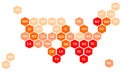
Fig. 4: Estimated centrality of 44 states in COVID-19 data. Deeper color indicates the state has a higher centrality.

Fig. 2 (Right), Fig. 3 plots the scoring functions $\Gamma(\widehat{\bm{v}}_{i})$ against the eigenvalue order $i$ for the 3 dataset considered. We first observe that the Stock data would satisfy ${\cal T}_{0}$ since $\Gamma(\widehat{\bm{v}}_{1})<\Gamma(\widehat{\bm{v}}_{j})$ for all $j\neq 1$, indicating that it is likely to be a set of first-order lowpass graph signals. This certifies that lowpass GSP tools can be applied to the dataset. For example, applying the method from [14, 15] ranks the centrality of stocks in the decreasing order as: NVDA, NFLX, AMZN, ADBE, PYPL, CAT, MA, GOOG, GOOGL, BA; see [14] for details. For the Senate data, we have $\Gamma(\widehat{\bm{v}}_{2})<\Gamma(\widehat{\bm{v}}_{j})$ for all $j\neq 2$ which suggests that the data may not be first-order lowpass. However, since the minimum occur at $\Gamma(\widehat{\bm{v}}_{2})$, it is plausible that the data is generated from a lowpass graph filter with cutoff frequency at $\lambda_{2}$. For the COVID-19 data, we see that $\Gamma(\widehat{\bm{v}}_{1})<\Gamma(\widehat{\bm{v}}_{j})$ for $2\leq j\leq 40$, yet $\Gamma(\widehat{\bm{v}}_{j})$ are small again for $j=41,...,44$. This suggests the sampled covariance has more than one (close-to) positive eigenvector. We suspect that this abnormally is due to outliers such as the beginning wave of a COVID-19 infection event at a state.

Inspired by the above, we model the COVID-19 data as a set of first-order lowpass graph signals (with outliers). Again, we can apply the blind centrality estimation method from [14, 15] to rank the centrality of states. The results are illustrated in Fig. 4. The top states ranked in decreasing centrality are FL, TX, CA, GA, LA, TN, SC, AL, NC, NY. Some of these states are the transportation hubs.

Conclusions. This paper utilizes the Perron-Frobenius theorem to design a simple, data-driven detector for identifying first-order lowpass graph signals. The detector can be used to provide certificates for applying lowpass GSP tools, and to make inference about the type of network dynamics. Future works include verifying 1, designing detectors for higher-order lowpass graph signals.

References

- [1] E. D. Kolaczyk and G. Csárdi, Statistical analysis of network data with R. Springer, 2014, vol. 65.
- [2] D. I. Shuman, S. K. Narang, P. Frossard, A. Ortega, and P. Vandergheynst, “The emerging field of signal processing on graphs: Extending high-dimensional data analysis to networks and other irregular domains,” IEEE signal processing magazine, vol. 30, no. 3, pp. 83–98, 2013.
- [3] A. Sandryhaila and J. M. F. Moura, “Discrete signal processing on graphs,” IEEE Transactions on Signal Processing, vol. 61, no. 7, pp. 1644–1656, 2013.
- [4] A. Ortega, P. Frossard, J. Kovačević, J. M. Moura, and P. Vandergheynst, “Graph signal processing: Overview, challenges, and applications,” Proceedings of the IEEE, vol. 106, no. 5, pp. 808–828, 2018.
- [5] D. Thanou, X. Dong, D. Kressner, and P. Frossard, “Learning heat diffusion graphs,” IEEE Transactions on Signal and Information Processing over Networks, vol. 3, no. 3, pp. 484–499, 2017.
- [6] W. Huang, T. A. Bolton, J. D. Medaglia, D. S. Bassett, A. Ribeiro, and D. Van De Ville, “A graph signal processing perspective on functional brain imaging,” Proceedings of the IEEE, vol. 106, no. 5, pp. 868–885, 2018.
- [7] H.-T. Wai, S. Segarra, A. E. Ozdaglar, A. Scaglione, and A. Jadbabaie, “Blind community detection from low-rank excitations of a graph filter,” IEEE Transactions on Signal Processing, vol. 68, pp. 436–451, 2019.
- [8] A. Sandryhaila and J. M. Moura, “Discrete signal processing on graphs: Frequency analysis,” IEEE Transactions on Signal Processing, vol. 62, no. 12, pp. 3042–3054, 2014.
- [9] R. Ramakrishna, H.-T. Wai, and A. Scaglione, “A user guide to low-pass graph signal processing and its applications,” IEEE Signal Processing Magazine, 2020.
- [10] V. Kalofolias, “How to learn a graph from smooth signals,” in Artificial Intelligence and Statistics, 2016, pp. 920–929.
- [11] X. Dong, D. Thanou, P. Frossard, and P. Vandergheynst, “Learning laplacian matrix in smooth graph signal representations,” IEEE Transactions on Signal Processing, vol. 64, no. 23, pp. 6160–6173, 2016.
- [12] H. E. Egilmez, E. Pavez, and A. Ortega, “Graph learning from data under laplacian and structural constraints,” IEEE Journal of Selected Topics in Signal Processing, vol. 11, no. 6, pp. 825–841, 2017.
- [13] B. Pasdeloup, V. Gripon, G. Mercier, D. Pastor, and M. G. Rabbat, “Characterization and inference of graph diffusion processes from observations of stationary signals,” IEEE transactions on Signal and Information Processing over Networks, vol. 4, no. 3, pp. 481–496, 2017.
- [14] Y. He and H.-T. Wai, “Estimating centrality blindly from low-pass filtered graph signals,” in ICASSP, 2020, pp. 5330–5334.
- [15] T. M. Roddenberry and S. Segarra, “Blind inference of centrality rankings from graph signals,” in ICASSP, 2020, pp. 5335–5339.
- [16] G. Mateos, S. Segarra, A. G. Marques, and A. Ribeiro, “Connecting the dots: Identifying network structure via graph signal processing,” IEEE Signal Processing Magazine, vol. 36, no. 3, pp. 16–43, 2019.
- [17] X. Dong, D. Thanou, M. Rabbat, and P. Frossard, “Learning graphs from data: A signal representation perspective,” IEEE Signal Processing Magazine, vol. 36, no. 3, pp. 44–63, 2019.
- [18] V. N. Ioannidis, Y. Shen, and G. B. Giannakis, “Semi-blind inference of topologies and dynamical processes over dynamic graphs,” IEEE Transactions on Signal Processing, vol. 67, no. 9, pp. 2263–2274, 2019.
- [19] H.-T. Wai, A. Scaglione, B. Barzel, and A. Leshem, “Joint network topology and dynamics recovery from perturbed stationary points,” IEEE Transactions on Signal Processing, vol. 67, no. 17, pp. 4582–4596, 2019.
- [20] B. Barzel and A.-L. Barabási, “Universality in network dynamics,” Nature physics, vol. 9, no. 10, pp. 673–681, 2013.
- [21] S. Segarra, G. Mateos, A. G. Marques, and A. Ribeiro, “Blind identification of graph filters,” IEEE Transactions on Signal Processing, vol. 65, no. 5, pp. 1146–1159, 2016.
- [22] Y. Zhu, F. J. I. Garcia, A. G. Marques, and S. Segarra, “Estimating network processes via blind identification of multiple graph filters,” IEEE Transactions on Signal Processing, vol. 68, pp. 3049–3063, 2020.
- [23] R. A. Horn and C. R. Johnson, Matrix analysis, 2nd ed. Cambridge university press, 2013.
- [24] D. Cvetkovic, S. Simic, and P. Rowlinson, An introduction to the theory of graph spectra. Cambridge University Press, 2009.
- [25] Y. Yu, T. Wang, and R. J. Samworth, “A useful variant of the davis–kahan theorem for statisticians,” Biometrika, vol. 102, no. 2, pp. 315–323, 2015.
- [26] R. Vershynin, High-dimensional probability: An introduction with applications in data science. Cambridge university press, 2018, vol. 47.
- [27] M. Fiedler, “A property of eigenvectors of nonnegative symmetric matrices and its application to graph theory,” Czechoslovak Mathematical Journal, vol. 25, no. 4, pp. 619–633, 1975.