A restless supermassive black hole in the galaxy J0437+2456

Abstract

We present the results from an observing campaign to confirm the peculiar motion of the supermassive black hole (SMBH) in J0437+2456 first reported in Pesce et al. (2018). Deep observations with the Arecibo Observatory have yielded a detection of neutral hydrogen (Hi) emission, from which we measure a recession velocity of 4910 km s^-1 for the galaxy as a whole. We have also obtained near-infrared integral field spectroscopic observations of the galactic nucleus with the Gemini North telescope, yielding spatially resolved stellar and gas kinematics with a central velocity at the innermost radii ($0.1^{\prime\prime}\approx 34$ pc) of 4860 km s^-1. Both measurements differ significantly from the $\sim$4810 km s^-1 H₂O megamaser velocity of the SMBH, supporting the prior indications of a velocity offset between the SMBH and its host galaxy. However, the two measurements also differ significantly from one another, and the galaxy as a whole exhibits a complex velocity structure that implies the system has recently been dynamically disturbed. These results make it clear that the SMBH is not at rest with respect to the systemic velocity of the galaxy, though the specific nature of the mobile SMBH – i.e., whether it traces an ongoing galaxy merger, a binary black hole system, or a gravitational wave recoil event – remains unclear.

1 Introduction

Given that nearly all galaxies are thought to harbor central supermassive black holes (SMBHs; Magorrian et al., 1998), interactions between SMBHs have long been recognized as a natural and perhaps inevitable byproduct of galaxy mergers. The two primary dynamical states that result from such interactions are SMBH binaries (Begelman et al., 1980; Roos, 1981) and gravitational recoil events (Fitchett, 1983; Redmount & Rees, 1989), both of which predict substantial nonequilibrium (“peculiar”) motion of the SMBH with respect to its surrounding environment. Yet despite much theoretical attention and observational effort, direct dynamical evidence for SMBH peculiar motion has remained elusive (see, e.g., Eracleous et al., 2012; Popović, 2012; Komossa & Zensus, 2016; Barack et al., 2019). In the absence of recent interactions with comparable-mass objects, an SMBH is expected to be in kinetic equilibrium with its surrounding environment (Merritt et al., 2007); for most SMBHs, the equilibrium velocity is $\ll 1$ km s^-1 with respect to the system barycenter.

Pesce et al. (2018, hereafter P18) presented a technique for using H₂O megamasers to measure SMBH peculiar motions. The key idea is that masers residing in the accretion disks around SMBHs (on scales of $\sim$0.1 pc) act as test particles whose dynamics can be used to probe the gravitational potential around the black hole, and very long baseline interferometric (VLBI) maps of the maser distribution enable precise (uncertainty ${\lesssim}10$ km s^-1) measurements of the SMBH’s line-of-sight velocity (e.g., Miyoshi et al., 1995; Kuo et al., 2011; Gao et al., 2017). P18 compared the maser-derived SMBH velocity measurements for 10 systems with independent estimates of their host galaxy velocities to constrain relative motions. One galaxy from the P18 sample – SDSS J043703.67+245606.8, hereafter J0437+2456 – showed a statistically significant (${>}5{\sigma}$) difference between the SMBH and host galaxy line-of-sight velocities; P18 thus identified J0437+2456 as a promising candidate for hosting either a recoiling or binary SMBH.

J0437+2456 is an approximately Sb-type spiral galaxy located at a distance of ${\sim}70$ Mpc (Greene et al., 2016; Pjanka et al., 2017). As measured by the Sloan Digital Sky Survey (SDSS), J0437+2456 has an $r$-band absolute AB magnitude of $M_{r}=-21.37$ and an estimated stellar mass of $7.2\times 10^{10}$ M_⊙. The megamaser system in J0437+2456 was mapped by Gao et al. (2017, hereafter G17), who also modeled the maser rotation curve and determined an SMBH velocity of $4818\pm 10.5$ km s^-1. P18 used a SDSS spectrum to measure the recession velocity of J0437+2456 to be $4887.6\pm 7.1$ km s^-1. The apparent $69.6\pm 12.7$ km s^-1 blueshift of the SMBH with respect to its host galaxy constitutes the putative peculiar motion. However, given the strong prior expectation for zero peculiar motion and the possibility that systematic effects such as SDSS fiber misalignment could plausibly account for a large fraction of the observed velocity difference, P18 cautioned that the peculiar motion measurement should be regarded as tentative pending corroborating observations.

In this paper we present the results from a followup observing campaign to confirm the peculiar motion of the SMBH in J0437+2456. This paper is organized as follows. In Section 2 we describe our observations and subsequent data reduction procedures, and in Section 3 we detail the velocity measurements made using these data. We discuss the results in Section 4, and we summarize and conclude in Section 5. Unless noted otherwise, all velocities quoted in this paper use the optical convention in the barycentric reference frame, and we assume a distance to J0437+2456 of 70 Mpc.

2 Observations and data reduction

In quiescent systems, Hi provides an appealing recession velocity tracer because it follows the global dynamics of the galaxy well outside of the SMBH sphere of influence and does not suffer from reddening or extinction. P18 targeted J0437+2456 with the Very Large Array (VLA) to observe neutral hydrogen (Hi), but no emission was detected within the six-hour integration time. We have obtained followup Hi observations of J0437+2456 using the Arecibo Observatory, which is much more sensitive than the VLA to low surface brightness emission but which lacks the ability to spatially resolve the gas distribution (see Figure 1). Our Arecibo observations are presented in Section 2.1.

Lacking Hi data, P18 measured the recession velocity for J0437+2456 using an SDSS spectrum. Like the Arecibo spectrum, the kinematics contributing to the SDSS spectrum are spatially unresolved within the 3-arcsecond aperture of the optical fiber used to transport light from the focal plane to the spectrograph (Gunn et al., 2006). However, because the aperture is smaller than the region containing the emitting material, the SDSS measurement is subject to an unknown amount of systematic uncertainty associated with the relative placement of the fiber center and the galactic nucleus. We have thus obtained followup high-resolution integral field spectra taken using the Gemini North telescope, which are able to spatially resolve the nuclear kinematics. Additionally, dust absorption should be weaker in the NIFS near-infrared waveband than at the SDSS optical wavelengths, so any velocity errors caused by patchy dust absorption will be smaller. Our Gemini observations are presented in Section 2.2.

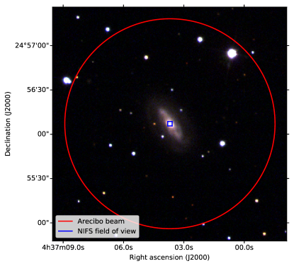
Figure 1: False-color image of J0437+2456 made by combining the $i$-, $r$-, and $g$-band observations from the SDSS Legacy Survey (York et al., 2000), with the 2.4-arcminute Arecibo beam and the $3^{\prime\prime}\times 3^{\prime\prime}$ NIFS field of view overplotted in red and blue, respectively.

2.1 Arecibo data

We performed Hi spectral-line observations of J0437+2456 over 6 nights using the Arecibo Observatory L-wide receiver. The observations were position-switched, with 5 minutes on and 5 minutes off source at matched elevation. We used the Wideband Arecibo Pulsar Processor (WAPP) spectrometer backend in single-polarization, 9-level autocorrelation mode with 4096 channels spanning the bandwidth 1384.5–-1409.5 MHz (i.e., $\pm$2500 km s^-1 centered on the Hi line). We used two such boards, one per polarization. Calibration diodes were observed at the end of every scan to determine the flux density scale.

Table 1 lists the on-source integration times for each of the 6 nights. With a declination of $+25$ degrees, J0437+2456 passes through the Arecibo observing window for ${\sim}2$ hours at a time. The position-switched observations thus yielded roughly an hour of on-source time per night.

We reduced the Arecibo data using AO IDL. We first converted the flux scale from K to Jy using the regular gain curve monitoring scans performed by the observatory (see Table 1). Each spectral scan was Hanning smoothed to mitigate ringing, and a fourth-order polynomial fit to the emission-free regions of the spectrum was subtracted off to remove low-frequency baseline ripples. We then combined each scan and both polarizations using an RMS-weighted average.

Figure 2 shows the Arecibo spectrum, in which we strongly detect Hi emission around the expected recession velocity range. The spectrum peaks at ${\sim}0.7$ mJy and has an integrated flux of ${\sim}$0.12 Jy km s^-1, consistent with the non-detection reported in P18. Assuming the Hi is optically thin, the total Hi mass is given by (Haynes et al., 2011; Condon & Ransom, 2016)

$$M_{\text{H{i}}}=\left(2.356\times 10^{5}\text{ M}_{\odot}\right)\left(\frac{D}{\text{Mpc}}\right)^{2}\left(\frac{\int S_{\nu}(v)dv}{\text{Jy\,km\,s${}^{-1}$}}\right),$$ (1)

where $D$ is the distance to the galaxy and $S_{\nu}(v)$ is the flux density as a function of velocity $v$. For a distance of 70 Mpc to J0437+2456, we estimate $M_{\text{H{i}}}\approx 1.4\times 10^{8}$ M_⊙ (see also Section 3).

Table 1: Arecibo observation details

	Integration	$\boldsymbol{T}_{\textbf{sys}}$	Gain
Date	(min.)	(K)	(K Jy-1)
2019 Jan 22	60	26.6	6.9
2019 Jan 23	65	26.8	6.9
2019 Jan 24	65	26.9	6.8
2019 Feb 11	60	27.1	7.0
2019 Feb 14	50	27.4	6.9
2019 Feb 17	50	27.0	6.9

Note. — Observing dates, on-source integration times, system temperatures, and gains for the Arecibo observations.

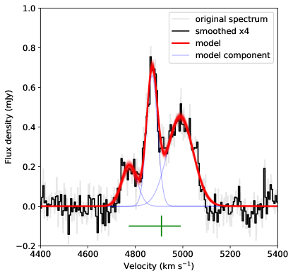
Figure 2: 1.4 GHz Arecibo spectrum towards J0437+2456. The spectrum is plotted with its native spectral resolution in gray, and the spectrum after smoothing by a 4-channel boxcar is shown in black. 1000 random posterior samples from a 3-component Gaussian model fit are overplotted in red, with the individual components for the best-fit model shown in blue. The measured $V_{20}$ velocity (see Section 3.1) is marked by a vertical green line, and the peak-to-peak velocity range is marked by a horizontal green line.

2.2 Gemini data

We obtained integral field spectra of a $3^{\prime\prime}\times 3^{\prime\prime}$ region centered on the nucleus of J0437+2456 using the Gemini North Near-Infrared Integral Field Spectrometer (NIFS) on 2018 November 21 in natural seeing mode. The spectrometer grating was set for K-band, with a central wavelength of 2.18 $\mu$m and spanning the range 1.99–2.41 $\mu$m. Nine 500-second exposures were taken, with five dithered exposures on-source and four offset to a blank sky location for subtraction. The observations were performed at airmasses of 1.2–1.6 and seeing conditions corresponding to a zenith-corrected point spread function of $\sim$0.3 arcseconds FWHM in $K$-band.

The NIFS data were reduced using the Gemini version 1.13 IRAF packages, with slight modifications to enable error array propagation and cube combination as described in Ahn et al. (2018). The resulting final data cube has a central signal-to-noise of $\sim$28, dropping to $\sim$10 at 0$\farcs$5 radius. Both strong stellar aborption lines and excited H₂ emission lines are seen, and their velocities are described in more detail in Section 3.2.

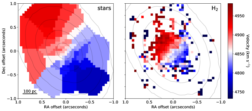
Figure 3: Velocity maps derived from the Gemini NIFS data within the central $2^{\prime\prime}\times 2^{\prime\prime}$ region. Left: Velocity map for the stellar component, using Voronoi binning such that each bin has a signal-to-noise ratio of at least 25. Right: H₂ velocity map. In both panels, mean continuum contours are overplotted at 5%, 10%, 20%, 40%, and 80% of the peak value.

3 Analysis

In this section we describe the analysis procedures used to measure velocities from the Arecibo spectrum (Section 3.1) and the Gemini spectra (Section 3.2).

3.1 Neutral hydrogen spectral decomposition and velocity measurements

Instead of the classic symmetric “double-horn” Hi profile (Roberts, 1978), J0437+2456 shows a more unusual triple-peaked and asymmetric spectral structure. Because our observations do not spatially resolve the Hi kinematics, the association of individual spectral properties with distinct dynamical components is ambiguous. While it is clear that a single double-horn component cannot describe the observed spectral profile, there are a variety of more complicated models that could potentially do so adequately. In Appendix A we explore three plausible model extensions, from which we conclude that the observed spectral structure is most conservatively and satisfactorily modeled using a sum of Gaussian components. Using the dynesty nested sampling routine (Speagle, 2020) to explore the posterior distribution, we find that $N=3$ Gaussian components are sufficient to capture the spectral structure and achieve a reduced-$\chi^{2}$ of $\sim$1 (see Figure 2); the velocities for these components are reported in Table 2 along with their statistical uncertainties. Our modeling procedure is described in more detail in Appendix A.

We use the modeled Hi spectrum to make a measurement of $V_{20}$, defined to be to the midpoint between the two points on the profile that rise to 20% of the peak amplitude (see, e.g., Fouque et al., 1990). $V_{20}$ provides an estimate of the galaxy recession velocity, and we find $V_{20}=4909.9\pm 1.9$ km s^-1. For the associated width of the profile, $W_{20}$, we find $W_{20}=326.0\pm 4.2$ km s^-1, and for the total mass of Hi we find $M_{\text{H{i}}}=(1.35\pm 0.18)\times 10^{8}$ M_⊙.

Table 2: Velocity measurements for different components in J0437+2456

Source of velocity	Velocity (km s-1)	Uncertainty (km s-1)	Spatial scale (pc)	Reference
Maser rotation curve	4818.0	10.5	0.2	G17
Maser rotation curve re-analysis	4809.3	10.0	0.2	this work
NIFS stellar	4857–4844	$\sim$2$\sim$	34–340	this work
NIFS H2	4858–4875	$\sim$2$\sim$	34–170	this work
NIFS integrated light	4865–4853	$\sim$2–4$\sim$	45–470	this work
SDSS spectrum, emission lines	4882.2	7.7	$1.0\times 10^{3}$	Pesce et al. (2018)
SDSS spectrum, stellar	4921.4	19.1		Pesce et al. (2018)
SDSS spectrum, average	4887.6	7.1		Pesce et al. (2018)
Hi spectrum, first component	4774.6	3.2	$4.9\times 10^{4}$	this work
Hi spectrum, second component	4870.2	0.8		this work
Hi spectrum, third component	4989.4	1.9		this work
Hi spectrum, $V_{20}$	4909.9	1.9		this work

Note. — Velocity measurements considered in this paper and the spatial scales on which they are measured, assuming a distance of 70 Mpc to J0437+2456. For the NIFS velocities, we quote the range of values corresponding to the systemic velocities at the innermost and outermost annuli in which measurements were made; note that for the NIFS stellar measurements, the systemic velocity measured from the outer annulus is smaller than that measured from the inner annulus. For the NIFS stellar and H₂ velocity measurements, the uncertainties are dominated by an overall calibration systematic of $\sim$2 km s^-1.

3.2 Systemic velocities of the stellar and H₂ components

The NIFS $K$-band spectra show both the strong stellar absorption lines of CO at $\sim$2.3 $\mu$m and molecular hydrogen emission lines, including the strong H₂ 1-0 S(1) line at rest wavelength 2.12 $\mu$m.

Stellar kinematics were derived by first Voronoi binning the data cube to $S/N\geq 25$ (Cappellari & Copin, 2003), and then fitting the data with pPXF (Cappellari & Emsellem, 2004) using high resolution stellar templates from Wallace & Hinkle (1996). The resulting radial velocity map can be seen in Figure 3. Errors on individual bins are determined through Monte Carlo simulations and range from 5–10 km s^-1. The velocity map was then analyzed using the Kinemetry code (Krajnović et al., 2006) to determine the barycentric systemic velocity as a function of radius from the observed photocenter; we note that the appearance of the galaxy in the NIFS data cubes is very symmetric. At the smallest radius (0$\farcs$05), the systemic velocity is 4856.8$\pm$1.6 km s^-1. Kinemetry reveals that the velocity steadily declines with radius – at 0$\farcs$5 it is 4844.5$\pm$0.6 km s^-1. These measurements are shown as orange dots in Figure 5. We note that the quoted errors are the formal errors produced by the Kinemetry code and are smaller than the systematic errors in our velocities discussed below.

To check the veracity of the systemic velocity shift with radius, we also binned the spectra in circular annular bins, and we ran pPXF on the resulting spectra. The mean velocity of the innermost spectrum ($<$0$\farcs$1) is 4865.4$\pm$2.9 km s^-1, while the annulus between 0$\farcs$4 and 0$\farcs$6 has a velocity of 4848.8$\pm$3.1 km s^-1. Thus it seems quite clear that there is indeed a blueshift in the systemic velocity of $\sim$15 km s^-1 between the center of the galaxy and the galaxy at radii of a few hundred parsecs. These “integrated light” measurements are shown as red points in Figure 5.

We also determine the kinematics of H₂ 1-0 S(1) emission line. Because the emission line strength does not follow the stellar emission distribution, for this measurement we do not bin the data, and instead we measure the velocities of the emission lines in each pixel with a Gaussian fit. We fit only lines where the total flux in our fitting region is $>$10 times the surrounding noise level. The result is shown in the right panel of Figure 3. Clear rotation with the same position angle as the stellar kinematics is visible. However, Kinemetry reveals that while the systemic velocities of the stellar and H₂ components are similar at the innermost radii, at larger radii the H₂ systemic velocity is actually redshifted (not blueshifted like the stellar kinematics), as shown by the blue points in Figure 5.

We note that the wavelength solution of the NIFS data was verified through fitting of sky lines in the spectra; a standard deviation of 1.1 km/s from the mean velocity was found from pixel to pixel, and an overall offset of -0.8 km/s was found. Thus the systematic errors on our velocity measurements are $<$2 km/s, much smaller than the velocity gradient observed in the stellar and gas kinematics.

3.3 The velocity of the SMBH

The velocity of the SMBH in J0437+2456 has previously been measured to be $4818\pm 10.5$ km s^-1 by G17, who used VLBI measurements of H₂O megamasers in the SMBH accretion disk to map out its rotation curve well within the gravitational sphere of influence. By fitting this rotation curve with a thin-disk Keplerian model, G17 were able to measure both the mass and velocity of the central SMBH. In this section, we re-analyze the same VLBI dataset using an updated maser disk model, which relaxes several of the assumptions made by G17 and thus permits an improved assessment of the associated velocity uncertainty.

The VLBI observations carried out by G17 resulted in position and velocity measurements for each of the detected maser features, or “spots.” G17 fit their rotation curve using a two-step procedure, in which the entire VLBI map is first rotated and shifted such that the blueshifted and redshifted masers lie on the horizontal axis, and then the maser spot velocities are fit as a function of their measured one-dimensional positions along this horizontal axis. The G17 rotation curve model contains three free parameters: the SMBH mass, the one-dimensional SMBH position along the horizontal axis, and the SMBH’s line-of-sight velocity.

For the present analysis we employ a modified version of the maser disk model described in Pesce et al. (2020) to fit the J0437+2456 VLBI data. The primary modification is the removal of acceleration measurements from the model likelihood, as the available VLBI dataset does not contain any such acceleration measurements. Our fitting approach differs from that of G17 in several respects:

1. We take the maser velocities, rather than their positions, to be the “independent” quantities; i.e., the model is essentially $r(v)$ rather than $v(r)$. This strategy leverages the fact that the individual velocity measurements are uncertain at a level comparable to a spectral channel width (${\sim}$1–2 km s^-1) and therefore much smaller than the orbital velocities of several hundred km s^-1, while the position uncertainties are comparatively large ($\sim$0.01–0.1 mas) relative to the orbital radii of several tenths of a milliarcsecond.

2. We do not perform any pre-rotation of the VLBI map, and instead we fit for the two-dimensional location of the SMBH on the sky along with the position angle of the disk.

3. We permit the disk inclination angle to be a free parameter in the fit.

4. We permit a warp in the position angle of the disk with radius.

5. We fit for systematic “error floor” parameters in the $x$ and $y$ maser position measurements alongside the disk model parameters. These error floor parameters describe the additional uncertainty that it would be necessary to add into the measurements to ensure that the data are consistent with the model; i.e., these parameters enforce a final reduced-$\chi^{2}$ value that is consistent with unity.

Detailed descriptions of the model parameters, likelihood, and fitting procedure are provided in Pesce et al. (2020). Following G17, we fit only to the redshifted and blueshifted maser features because there are no available acceleration measurements to constrain the systemic maser feature orbital radii. The final model contains 9 parameters, which are listed in Table 3 along with their priors and best-fit values.

Table 3: Results from re-analysis of maser VLBI data

Parameter	Units	Prior	Best-fit value
v_0	km s-1	U(4500,5500)	4809.3 ±10.0
M	$10^{6}$ $\text{M}_{\odot}$	U(0,30)	2.86 ±0.2
x_0	mas	U(-0.5,0.5)	0.096 ±0.005
y_0	mas	U(-0.5,0.5)	0.109 ±0.014
i_0	deg.	U(70,110)	unconstrained
Ω_0	deg.	U(0,180)	16.9 ±2.5
Ω_1	deg. mas-1	U(-100,100)	14 ±8
σ_x	$\mu$as	U(0,1000)	6 ±1.5
σ_y	$\mu$as	U(0,1000)	¡5

Note. — Results from fitting a thin Keplerian disk model to the J0437+2456 VLBI maser dataset from G17, as described in Section 3.3 and shown in Figure 4. The fitted model parameters are the SMBH velocity $v_{0}$, the SMBH mass $M$, the SMBH position $(x_{0},y_{0})$, the disk inclination $i_{0}$, the disk position angle $\Omega_{0}$, a first-order warp in the disk position angle with radius $\Omega_{1}$, and two error floor parameters $\sigma_{x}$ and $\sigma_{y}$ for the maser $x$- and $y$-position measurements, respectively. The notation $\mathcal{U}(a,b)$ denotes a uniform distribution on the range $(a,b)$. For most parameters we report the posterior mean and standard deviation, though we note that the $\sigma_{y}$ parameter has a best-fit value that is consistent with zero and so we report the 95% upper limit instead. For the $i_{0}$ parameter, the posterior distribution matches the prior distribution, and so we do not report constraints on this parameter. A more detailed description of the various model parameters can be found in Pesce et al. (2020).

Our best-fit rotation curve and disk model are shown in Figure 4, from which we determine the SMBH velocity to be $4809.3\pm 10.0$ km s^-1. We find that the uncertainty in the derived velocity matches well with the result from G17, though our best-fit velocity itself is approximately 9 km s^-1 smaller. Because our disk model relies on fewer assumptions than that employed in G17, we hereafter adopt $4809.3\pm 10.0$ km s^-1 as the velocity measurement of the SMBH in J0437+2456.

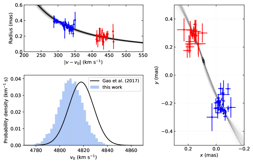
Figure 4: Results from fitting a thin Keplerian disk model to the J0437+2456 maser measurements from G17; the best-fit model parameters are listed in Table 3. The top left panel shows the on-sky projected radial separation from the SMBH versus orbital velocity for each of the maser spots, with the best-fit rotation curve plotted in black and 200 draws from the posterior distribution plotted in gray. The points corresponding to individual maser features have been colored by velocity group, with blue points denoting blueshifted maser features and red points denoting redshifted maser features. The bottom left panel shows the posterior distribution for the SMBH velocity that we obtain from our fitting procedure (blue histogram) along with a Gaussian distribution with the mean and standard deviation reported in G17 (black line). The right panel shows the VLBI map of the maser system, with the best-fit warped disk midplane plotted as a dashed line and 200 draws from the posterior distribution plotted as solid gray lines; the 1$\sigma$ and 2$\sigma$ contours for the SMBH location are shown as thick and thin black ellipses, respectively.

4 Discussion

The recession velocity measurements considered in this paper are listed in Table 2, and they are plotted against spatial scale in Figure 5. We find that all velocity measurements fall within a $\sim$100 km s^-1 range spanning ${\sim}$4820–4920 km s^-1, and there is a general trend for measurements made at larger spatial scales to recover larger recession velocities. In this section we discuss the various measurements and consider some possible interpretations.

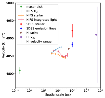
Figure 5: The spatial scales on which the various velocity measurements considered in this paper are made. For the Hi spike, we take the spatial scale to be $\geq$600 pc as implied by the brightness temperature limit given in Equation 2. The full peak-to-peak velocity range spanned by the Hi emission (corresponding to the horizontal green line at the bottom of Figure 2) is shown as a vertical line that is horizontally offset from the $V_{20}$ velocity for visual clarity. For the NIFS measurements, we plot the systemic velocities as a function of annulus diameter and we include an overall 2 km s^-1 calibration systematic uncertainty on the error bars. All other velocities are plotted with statistical error bars.

4.1 Velocity measurements in J0437+2456

The largest spatial scales are probed by the Hi emission, which traces gas throughout the galaxy and out to the edge of the Arecibo beam (roughly $\sim$50 kpc across). J0437+2456’s Hi profile is atypical in that it shows three prominent spectral peaks rather than the usual two that are expected for a simply-rotating system. Similar profiles have been classified as “anomalous” by previous authors (e.g., UGC 2889 in Courtois et al., 2009), and they are often attributed to spatial blending of galaxy pairs in single-dish spectra, such as in the case of NGC 876 and NGC 877 (Bottinelli et al., 1982; Lee-Waddell et al., 2014). However, for J0437+2456 we see neither evidence for a companion galaxy within the Arecibo beam (see Figure 1) nor obvious signs of morphological disturbance in Hubble Space Telescope (HST) images (Pjanka et al., 2017). Nevertheless, the measured Hi central velocity of $V_{20}=4910$ km s^-1 is in agreement with the SDSS stellar velocity measured by P18, supporting the notion that both measurements trace the recession velocity of J0437+2456. Furthermore, the Hi central velocity is in ${\sim}10{\sigma}$ disagreement with the SMBH velocity as measured from the maser rotation curve (Section 3.3), indicating that the black hole is blueshifted by roughly 100 km s^-1 with respect to the galaxy’s recession velocity.

The NIFS measurements probe spatial scales of $\sim$30–300 pc. The sense of rotation for both the stellar and H₂ components agrees with that of the maser disk (G17), though the maser disk has a position angle of ${\sim}20^{\circ}$ while the outermost stellar and H₂ components have position angles of ${\sim}40^{\circ}$. We find that the systemic velocities of the stellar and H₂ rotation curves agree with one another on the smallest scales ($\sim$30 pc), though they both show a $\sim$4.7$\sigma$ redshift with the respect to the maser velocity. At larger radii the stellar and H₂ systemic velocity measurements diverge, with the stellar systemic velocity showing a $\sim$30 km s^-1 blueshift with respect to the H₂ on scales of $\sim$200 pc. Such large variations in the measured stellar systemic velocity as a function of radius are rare; the typical dispersion of ATLAS${}^{\text{3D}}$ galaxies between the central and $r=500$ pc velocities is only $\sim$3–4 km s^-1 (Appendix B; Krajnović et al. 2011), and most of the galaxies with substantially larger systemic velocity gradients show evidence of interaction. We note, however, that such a relative velocity offset could also be plausibly explained by a combination of geometric and obscuration effects (e.g., if the stellar and $H_{2}$ emission arose from two separate misaligned and mutually obscuring disks of material) while leaving the system dynamically relaxed, and that the structure maps produced by Pjanka et al. (2017) do show evidence of dust on $\sim$0.3^′′ and larger scales.

The outermost H₂ emission ($\sim$200 pc) has a systemic velocity of 4875 km s^-1 that matches well with the emission line velocity measured by P18 from the SDSS spectrum, indicating that these two measurements may be tracing similar material. These measurements are both also in agreement with the velocity of the “anomalous” central Hi spike, which has a velocity of $\sim$4870 km s^-1 and an amplitude of $S_{\nu}\approx 0.7$ mJy (see Table 4). If this Hi spike represents a distinct dynamical subsystem (rather than, e.g., one “horn” of a double-horn profile), then we can set a lower limit on the area of the emission region by requiring that the Hi brightness temperature not exceed its spin temperature of $T_{s}\approx 150$ K (Condon & Ransom, 2016),

$$\Omega\geq\frac{S_{\nu}c^{2}}{2k\nu^{2}T_{s}}.$$ (2)

Here, $k$ is the Boltzmann constant, $\nu=1.4$ GHz is the emitting frequency, and $\Omega$ is the solid angle subtended by the emitting region. Equation 2 implies that the angular size of the region contributing the Hi spike is ${\sim}1.8^{\prime\prime}\approx 600$ pc. This spatial scale is similar to that probed by the NIFS observations, and together with the coincident velocities suggests that all three sources of emission – i.e., the outermost H₂, the SDSS emission lines, and the Hi spike – may be originating from material with shared dynamics. The velocity of this material is significantly different from that of both the SDSS stellar and the central Hi velocity (i.e., $V_{20}$), perhaps indicating that there is a kinematically distinct subsystem located in the centermost few hundred parsecs of J0437+2456. However, we note that the observed FWHM of the Hi spike of only $\sim$55 km s^-1 (see Table 4) is in tension with this interpretation, because at several-hundred parsec radii the material in this galaxy should display a FWHM of $\sim$200 km s^-1 (Figure 3; see also Noordermeer et al. 2007). It thus may not be viable to interpret this Hi spike as a distinct kinematic component.

4.2 Uncertainty in the black hole velocity measurement

Our measurement of the SMBH velocity (see Section 3.3) relies on accurate VLBI position measurements for each of the maser features, and if there are unaccounted-for systematic uncertainties in these position measurements then we would expect the velocity measurement to be correspondingly impacted. G17 considered the impact of phase referencing uncertainties on the J0437+2456 maser position measurements. The absolute sky location of the J0437+2456 peak maser emission (i.e., the emission at a velocity of 4505.8 km s^-1 used as a reference feature) is known from phase-referenced VLBI measurements to a precision of better than 2 mas. G17 estimate that the expected additional positional uncertainties associated with this imperfectly-known reference position, when propagated to the rest of the maser features, should be ${\lesssim}$5 $\mu$as. This expectation is consistent with the magnitudes of the error floor parameters that we recover from our model fitting (see Table 3). Additionally, we note that there are no obvious systematic trends in the residual dispersion about the best fit such as would be expected if poor phase calibration were present at this level.

4.3 An offset black hole

In our own Galactic Center, we have high-precision evidence that the SMBH is coincident with the dynamical center of the Galaxy (Reid & Brunthaler, 2020). While we believe that a similar situation should generally hold for other galaxies as well, a number of effects can at least temporarily knock the SMBH out of this equilibrium position. At very low galaxy mass, it is possible that SMBHs never settle at their galaxy center, given the very shallow galactic potential (e.g., Bellovary et al., 2019; Reines et al., 2020). However, at higher galaxy masses, it is most likely that mergers are responsible for SMBH motions.

Relative motions and spatial offsets between SMBHs and their host galaxies occur throughout the merger process. As galaxies merge, the SMBHs from each galaxy will be offset both spatially and in velocity from the center of the merger. This stage may be observable as velocity offset active galaxies (e.g., Comerford et al., 2009; Comerford & Greene, 2014) or as spatially resolved pairs of active galactic nuclei (AGN; e.g., Komossa et al. 2003; Gerke et al. 2007). Further along in the merger process, when the two SMBHs become gravitationally bound, one may hope to observe the signatures of orbital motion for the bound pair (e.g., Eracleous et al., 2012; Shen et al., 2013; Ju et al., 2013, see also Appendix C). Finally, if an SMBH merger occurs, then any anisotropy in the radiated linear momentum will lead to a gravitational wave recoil (Fitchett, 1983). These have been many observational recoil candidates proposed, but all have their complications (see reviews in Komossa 2012 and Blecha et al. 2016).

The SMBH in the galaxy J0437+2456 is, to our knowledge, the most concrete case of an SMBH in motion with respect to its galaxy. Because our initial search focused on megamaser disk galaxies (P18), the sources were all within 200 Mpc where detailed followup observations are possible; luminous AGN that have been identified as recoil or binary SMBH candidates in the past are often much more distant. Even in the case of J0437+2456, ambiguity remains about whether we are seeing an SMBH making its way to the galaxy center for the first time, SMBH binary orbital motion, or a recoil product. However, the fact that the galaxy on large scales is apparently out of equilibrium provides indirect evidence that we are observing the aftermath of a merger.

5 Summary and conclusion

Following the identification in P18 of the galaxy J0437+2456 as a candidate for hosting a binary or recoiling SMBH, we have obtained Arecibo and Gemini NIFS observations of the galaxy. Our new observations support the claim of a velocity offset between the SMBH and its host galaxy. Furthermore, the systemic velocity in J0437+2456 exhibits an apparent spatial scale dependence; the overall picture looks something like the following:

1. On the smallest spatial scales ($<$1 pc), where the motion of gas is dominated by the gravitational potential of the SMBH, H₂O masers orbit with a central velocity of $\sim$4810 km s^-1. We associate this velocity with the SMBH itself.

2. At the photocenter of the galaxy, within the central $\sim$30 pc and coincident with the location of the SMBH, both the stars and H₂ gas emission lines have a systemic velocity of $\sim$4860 km s^-1. However, on somewhat larger scales ($\sim$30–200 pc), both gas and stars exhibit unusual systemic velocity gradients of $\sim$15 km s^-1 in opposite directions. In all cases, these velocities are significantly offset from the SMBH velocity as traced by the masers.

3. On the largest spatial scales ($\sim$1–10 kpc), the velocity of the Hi emission is in agreement with the SDSS stellar velocity from P18. We find a central Hi velocity of $V_{20}\approx 4910$ km s^-1 that we associate with the recession velocity of the galaxy as a whole, though we note that the “anomalous” structure of the Hi spectral profile complicates this interpretation.

Multiple lines of evidence – including the different inferred systemic velocities on different spatial scales, the “anomalous” Hi spectral structure, and the gradient in stellar systemic velocity with radius – point to the conclusion that the galaxy J0437+2456 has been dynamically perturbed sometime in the recent past, likely through an interaction with another galaxy. Of particular interest is the apparent difference between the systemic velocity of the SMBH and that of any other dynamical tracer, indicating that the SMBH in this galaxy is in motion with respect to the surrounding material.

P18 explored plausible causes of such relative motion, ultimately settling on three possibilities: (1) the SMBH originates from an external galaxy that is in the process of merging with J0437+2456; (2) the SMBH is part of a binary system, and the velocity offset we observe is the result of its orbital motion; or (3) the SMBH is recoiling from a recent merger event. Though any of these possibilities would be exciting, with the current data we are unfortunately unable to distinguish between them. Additional observations are required to ascertain the nature of the peculiar SMBH in J0437+2456.

Appendix A Hi spectral modeling

Here we describe three different models we use to fit the Hi spectrum from Section 3.1. For each model, we use a Gaussian likelihood given by

$$\ln\left(\mathcal{L}\right)=-\frac{1}{2}\sum_{j}\left[\left(\frac{S_{\nu}(v_{j})-\hat{S}_{\nu}(v_{j})}{\sigma}\right)^{2}+\ln\left(2\pi\sigma^{2}\right)\right],$$ (A1)

where $S_{\nu}(v_{j})$ is the model flux density for a spectral channel with velocity $v_{j}$, $\hat{S}_{\nu}(v_{j})$ is the observed flux density in that channel, $\sigma$ is the flux density uncertainty in a single channel, and the sum is taken over all channels. This likelihood assumes that every spectral channel contains independent Gaussian-distributed noise with a standard deviation $\sigma$ that we treat as a model parameter in each of our fits. We use the dynesty nested sampling code (Speagle, 2020) for posterior exploration. The best-fit values and uncertainties for all model parameters are listed in Table 4.

A.1 Modeling the profile using a sum of Gaussian components

The model we use in our primary analysis (Section 3.1) describes the Hi spectral structure using a sum of Gaussian components,

$$S_{\nu}(v)=\sum_{i=1}^{N}A_{i}\exp\left[-\frac{1}{2}\left(\frac{v-v_{i}}{\sigma_{i}}\right)^{2}\right],$$ (A2)

where the model parameters are the amplitude $A_{i}$, central velocity $v_{i}$, and width $\sigma_{i}$ for each component. The total number of model parameters is $3N+1$, where $N$ is the number of Gaussian components; in this paper, we use $N=3$. We impose uniform priors on all model parameters, in the range $[0,1]$ mJy for Gaussian component amplitudes, $[0,500]$ km s^-1 for all Gaussian component standard deviations, $[4500,5300]$ km s^-1 for all Gaussian component central velocities, and $[0,1]$ mJy for $\sigma$. The posterior distribution is trivially multimodal upon pairwise swaps of Gaussian components, but the modes are widely separated in parameter space and so we isolate a single mode when reporting parameter statistics. A plot of the resulting fit to the spectrum is shown in the left panel of Figure 6.

Table 4: Results from Hi spectral modeling

Model description	Parameter description	Units	Best-fit value
three Gaussian components	central velocity of first component	km s-1	4774.6 ±3.2
	central velocity of second component	km s-1	4870.2 ±0.8
	central velocity of third component	km s-1	4989.4 ±1.9
	FWHM of first component	km s-1	76.4 ±6.4
	FWHM of second component	km s-1	54.6 ±2.3
	FWHM of third component	km s-1	129.0 ±4.1
	amplitude of first component	mJy	0.20 ±0.01
	amplitude of second component	mJy	0.66 ±0.02
	amplitude of third component	mJy	0.45 ±0.01
	thermal noise level (RMS)	mJy	0.068 ±0.002
two double-horn components	central velocity of first component	km s-1	4810.7 ±2.0
	central velocity of second component	km s-1	4955.9 ±2.8
	velocity width of first component	km s-1	139.6 ±4.2
	velocity width of second component	km s-1	234.0 ±9.4
	flux of first component	mJy km s-1	51.7 ±3.5
	flux of second component	mJy km s-1	97.6 ±2.6
	asymmetry of first component	unitless	0.46 ±0.09
	asymmetry of second component	unitless	0.38 ±0.07
	solid-body fraction of first component	unitless	0.03 ±0.03
	solid-body fraction of second component	unitless	0.89 ±0.07
	velocity dispersion of first component	km s-1	12.0 ±1.2
	velocity dispersion of second component	km s-1	11.0 ±3.1
	thermal noise level (RMS)	mJy	0.064 ±0.002
one double-horn component and one Gaussian component	central velocity of double-horn component	km s-1	4904.1 ±3.7
	velocity width of double-horn component	km s-1	312.5 ±10.2
	flux of double-horn component	mJy km s-1	124.3 ±3.2
	asymmetry of double-horn component	unitless	0.61 ±0.05
	solid-body fraction of double-horn component	unitless	0.63 ±0.14
	velocity dispersion of double-horn component	km s-1	18.5 ±5.9
	central velocity of Gaussian component	km s-1	4870.9 ±0.7
	FWHM of Gaussian component	km s-1	38.1 ±2.1
	amplitude of Gaussian component	mJy	0.47 ±0.02
	thermal noise level (RMS)	mJy	0.066 ±0.002

Note. — Results from fitting the three different models described in Appendix A to the Arecibo Hi spectrum; these fits are shown in Figure 6. For each parameter, we quote the posterior mean and standard deviation. The thermal noise has been determined per 61 kHz ($\approx$1.33 km s^-1) spectral channel.

A.2 Modeling the profile using a sum of double-horn components

Given that the galaxy J0437+2456 shows signs of dynamical disturbance (potentially indicating a recent merger) and that it exhibits an “anomalous” Hi profile (Figure 2), it is natural to ask whether a combination of double-horn profiles could give rise to the observed spectral structure. We have thus performed an alternative analysis using a sum of two double-horn components, each described using the parameterization developed by Stewart et al. (2014) for each component.

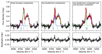
Figure 6: Similar to Figure 2, but showing the results of fits using the three different classes of model described in Appendix A; the best-fit parameter values for each model are listed in Table 4. In the left panel we show a more detailed breakdown of the fit from Figure 2 using three Gaussian components, with the individual best-fit Gaussian model components plotted in blue, green, and violet. Their corresponding best-fit velocities are marked by the vertical lines underneath each component. In the center panel we show a similar breakdown for the fit using two double-horn components, and in the right panel the fit using one double-horn component and one Gaussian component. In all panels, the spectrum is plotted at its native spectral resolution in gray, the spectrum after smoothing by a 4-channel boxcar is shown in black, and 1000 random posterior samples are overplotted in red. The bottom row of plots shows the residuals (i.e., the difference between the data and best-fitting model) for each fit.

The Stewart et al. (2014) model describes a double-horn profile using six parameters: the total flux, the central velocity, the velocity width, an asymmetry parameter, a parameter describing what fraction of the emission comes from solid-body rotation, and a velocity dispersion. Because we model the spectrum as a sum of $N$ such double-horn components, and because we additionally model the channel uncertainty $\sigma$, the total number of model parameters is $6N+1$; in this paper, we use $N=2$. We impose uniform priors on all model parameters, in the range $[0,1]$ Jy km s^-1 for the total flux, $[4500,5300]$ km s^-1 for the central velocity, $[0,600]$ km s^-1 for the velocity width, $[-1,1]$ for the asymmetry parameter, $[0,1]$ for the solid-body fraction, $[0,100]$ km s^-1 for the velocity dispersion, and $[0,1]$ mJy for $\sigma$.

The results of fitting this alternative model to the Hi data are shown in the central panel of Figure 6. We find that the best-fit model prefers only one of the two components to exhibit a standard double-horn profile, while the other component is dominated by the solid-body contribution and so has only a single, wide spectral peak. This model struggles to fit the central Hi spike, as evidenced by the large residual flux excess near $\sim$4850 km s^-1, so we disfavor it compared to the model composed of three Gaussian components.

A.3 Modeling the profile using a sum of double-horn and Gaussian components

Motivated by the appearance of the Hi spectrum, we also attempt to model it using a sum of one double-horn component (parameterized as in Stewart et al. 2014 and Section A.2) and one Gaussian component. The resulting parameter values are listed in Table 4 and the best-fit spectrum is plotted in Figure 6. We again find that even the best-fit model struggles to fit the observed spectral profile, with a substantial flux excess seen in the residuals around $\sim$4750 km s^-1. We thus disfavor this model compared to the model composed of three Gaussian components.

Appendix B ATLAS${}^{\text{3D}}$ systemic velocity curves

The ATLAS${}^{\text{3D}}$ project has collected integral field spectroscopic measurements for a sample of 260 early-type galaxies in the local Universe (Cappellari et al., 2011). This sample provides a reference against which we can gauge the behavior of the NIFS stellar systemic velocity measurements for J0437+2456, which show a systematic trend with radius (see Section 3.2).

Figure 7 shows the radial profile of the J0437+2456 stellar systemic velocity measurements plotted alongside the same quantity measured for the “fast rotator” galaxies from ATLAS${}^{\text{3D}}$. The ATLAS${}^{\text{3D}}$ sample is made up of early-type galaxies, while J0437+2456 is a spiral, so for comparison we select only fast rotators from the ATLAS${}^{\text{3D}}$ sample because they are galaxies with high angular momentum (Emsellem et al., 2011), stellar disks, and ordered (i.e., disk-like) stellar kinematics (Krajnović et al., 2011, 2013). We note that unlike the $\sim$0.3-arcsecond seeing of our NIFS observations (see Section 2.2), many of the ATLAS${}^{\text{3D}}$ observations were carried out under $\sim$1–2-arcsecond seeing conditions (Emsellem et al., 2004) and so the innermost radial points of each profile in Figure 7 may suffer accordingly. Nevertheless, we see that the steep rise of the systemic velocity with radius, as well as the large difference in systemic velocities as measured at small and large radii, are both considerably more extreme in J0437+2456 than in the majority of ATLAS${}^{\text{3D}}$ galaxies. At about 200 pc from the center the systemic velocity of a typical fast rotator deviates by only $\sim$2-3 km s^-1 from the systemic velocity measured near the center. This trend does not change substantially with increasing radius.

There are a few galaxies in the ATLAS${}^{\text{3D}}$ sample that have systemic velocity deviations similar to or even larger than those seen in J0437+2456, albeit at larger radii. The galaxies with the top four largest deviations are labeled in Figure 7: NGC 4753, UGC 09519, NGC 4342 and NGC 3665. NGC 4753, which has the largest difference in the systemic velocity, also shows clear morphological evidence of a recent merger and contains complex dust filaments (Krajnović et al., 2011; Bílek et al., 2020), indicating that it is likely not in equilibrium. UGC 09519 might be dusty in the center, and it also has an unusual large-scale stellar disk characterised by blue colours and low surface brightness (Duc et al., 2015). NGC 3665 has a well defined nuclear dust and gas disk (Onishi et al., 2017), as well as asymmetric outer isophotes (Bílek et al., 2020). NGC 4342 shows no evidence for disturbances in morphology or kinematics, except harbouring a central nuclear stellar disk (Scorza & van den Bosch, 1998), though Cretton & van den Bosch (1999) note that this galaxy has a remarkably large central velocity dispersion for its size and luminosity. The ATLAS${}^{\text{3D}}$ sample is perhaps not an ideal comparison sample, as it is made of early-type galaxies and the observations do not probe the same spatial scales as the NIFS data of J0437+2456. Nevertheless, it is clear that the majority of ATLAS${}^{\text{3D}}$ galaxies do not show strong variations in systemic velocity with radius, and there is some evidence that those with strong variations tend to exhibit other indications of kinematic disturbance.

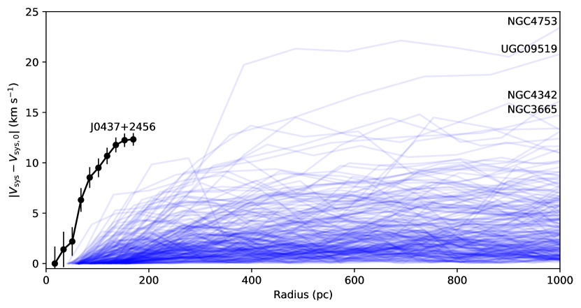
Figure 7: The radial profile of the J0437+2456 systemic velocity as measured from the NIFS stellar emission (plotted in black; see Section 3.2) compared against similar profiles for “fast rotator” galaxies from ATLAS${}^{\text{3D}}$ (plotted in blue). For each galaxy, we have subtracted off the systemic velocity measured at the smallest radii ($V_{\text{sys},0}$) and then taken an absolute value of the difference to aid comparison.

Appendix C Observational constraints on the properties of a hypothetical binary SMBH system in J0437+2456

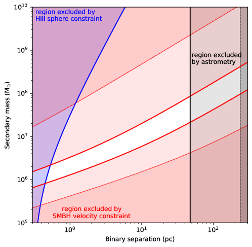
Figure 8: Observational constraints on the space of secondary SMBH mass and binary separation for J0437+2456. The blue shaded region is excluded by the requirement that the observed maser disk be tidally undisrupted, the red shaded region is excluded by the requirement that the observed SMBH exhibit the measured velocity offset, and the gray shaded region is excluded by the lack of an astrometric offset seen between the SMBH and the galactic center. The remaining unshaded region indicates the permitted range of secondary SMBH mass and binary separation in the presence of these constraints. For the red and gray shaded regions, the solid and dashed lines represent 50% and 90% probability bounds, respectively, determined as described in Appendix C.

We observe the SMBH in J0437+2456 to have a velocity offset with respect to its host galaxy, as determined using various different systemic velocity tracers (see Section 4.1). One possible explanation for this velocity offset is that the observed SMBH is part of a binary black hole system with a second, unseen SMBH. In this case, we have several observational constraints on the properties that such a binary system must have; these constraints are illustrated in Figure 8.

Our first constraint comes from the fact that the observed SMBH in J0437+2456 is surrounded by an accretion disk, which is traced by H₂O maser emission to extend out to radii of $\sim$0.3 pc ( G17, see also the right panel of Figure 4). If a second SMBH is present outside of this accretion disk, then its mass and separation from the observed SMBH must be such that it avoids tidally disrupting the accretion disk. This condition is roughly equivalent to requiring that the outer edge of the accretion disk lie within the Hill sphere of the observed SMBH. If we denote the mass of the observed SMBH as $m_{1}$, the mass of the second SMBH as $m_{2}$, their separation as $r$, and the Hill sphere radius as $r_{H}$, then we can cast this condition as an upper bound on $m_{2}$ of

$$m_{2}\leq\frac{m_{1}}{r_{H}^{2}}\left[\frac{1}{\left(r-r_{H}\right)^{2}}-\frac{1}{r^{2}}\right]^{-1}.$$ (C1)

The blue shaded region in Figure 8 shows the combinations of $m_{2}$ and $r$ that are excluded by this criterion. We use the measured value of $m_{1}=2.9\times 10^{6}$ M_⊙ from G17 for the mass of the observed SMBH and the aforementioned value of $r_{H}=0.3$ pc from the VLBI map.

Our second constraint comes from the observed velocity offset of the SMBH with respect to the host galaxy. If this SMBH is participating in a binary system, then its line-of-sight velocity $v$ is related to the parameters of the binary orbit via (see, e.g., Murray & Dermott, 1999)

$$v=m_{2}\sin(i)\big{[}\cos(\omega+f)+e\cos(\omega)\big{]}\sqrt{\frac{2G}{r\left(1-e^{2}\right)\left(m_{1}+m_{2}\right)}}.$$ (C2)

Here, $i$ is the inclination of the orbital plane, $\omega$ is its argument of pericenter, $f$ is the true anomaly of the observed SMBH, and $e$ is the orbital eccentricity; $m_{1}$, $m_{2}$, and $r$ are the same as in Equation C1. We do not currently have any ability to constrain the geometric parameters of the orbit, so we instead treat them probabilistically; we assume that the orbital plane is oriented randomly on the sphere (i.e., $\omega$ is distributed uniformly on $[0,2\pi]$ and $\cos(i)$ is distributed uniformly on $[-1,1]$), that $f$ is oriented randomly on the circle, and that $e$ is distributed uniformly in the range $[0,1]$. The solid and dashed red lines in Figure 8 show the 50% and 90% probability contours, respectively, for the combined constraints on $m_{2}$ and $r$ given these assumptions about the distribution of possible orbit geometries. For the purposes of this constraint, we estimate the orbital velocity of the SMBH in J0437+2456 to be $48\text{\,km\,s${}^{-1}$}\leq v\leq 101$ km s^-1 based on the measurements presented in this paper (see Table 2).

Our third and final constraint comes from the apparent lack of an astrometric offset between the SMBH in J0437+2456 and the center-of-light, determined in P18 to be $\lesssim$0.05 arcseconds. If we take this value to be an upper limit on the SMBH binary on-sky separation, then we can convert it into a constraint on the SMBH binary absolute separation. We are again faced with the fact that we do not have any handle on the orientation of the binary orbit, so we assume that the orbit is randomly distributed on the sphere and plot 50% and 90% probability regions in Figure 8 (shown as light and dark gray shaded regions, respectively).

References

- Ahn et al. (2018) Ahn, C. P., Seth, A. C., Cappellari, M., et al. 2018, ApJ, 858, 102, doi: 10.3847/1538-4357/aabc57
- Barack et al. (2019) Barack, L., Cardoso, V., Nissanke, S., et al. 2019, Classical and Quantum Gravity, 36, 143001, doi: 10.1088/1361-6382/ab0587
- Begelman et al. (1980) Begelman, M. C., Blandford, R. D., & Rees, M. J. 1980, Nature, 287, 307, doi: 10.1038/287307a0
- Bellovary et al. (2019) Bellovary, J. M., Cleary, C. E., Munshi, F., et al. 2019, MNRAS, 482, 2913, doi: 10.1093/mnras/sty2842
- Bílek et al. (2020) Bílek, M., Duc, P.-A., Cuilland re, J.-C., et al. 2020, MNRAS, 498, 2138, doi: 10.1093/mnras/staa2248
- Blecha et al. (2016) Blecha, L., Sijacki, D., Kelley, L. Z., et al. 2016, MNRAS, 456, 961, doi: 10.1093/mnras/stv2646
- Bottinelli et al. (1982) Bottinelli, L., Gouguenheim, L., & Paturel, G. 1982, A&AS, 50, 101
- Cappellari & Copin (2003) Cappellari, M., & Copin, Y. 2003, MNRAS, 342, 345, doi: 10.1046/j.1365-8711.2003.06541.x
- Cappellari & Emsellem (2004) Cappellari, M., & Emsellem, E. 2004, PASP, 116, 138, doi: 10.1086/381875
- Cappellari et al. (2011) Cappellari, M., Emsellem, E., Krajnović, D., et al. 2011, MNRAS, 413, 813, doi: 10.1111/j.1365-2966.2010.18174.x
- Comerford & Greene (2014) Comerford, J. M., & Greene, J. E. 2014, ApJ, 789, 112, doi: 10.1088/0004-637X/789/2/112
- Comerford et al. (2009) Comerford, J. M., Gerke, B. F., Newman, J. A., et al. 2009, ApJ, 698, 956, doi: 10.1088/0004-637X/698/1/956
- Condon & Ransom (2016) Condon, J. J., & Ransom, S. M. 2016, Essential Radio Astronomy (Princeton University Press)
- Courtois et al. (2009) Courtois, H. M., Tully, R. B., Fisher, J. R., et al. 2009, AJ, 138, 1938, doi: 10.1088/0004-6256/138/6/1938
- Cretton & van den Bosch (1999) Cretton, N., & van den Bosch, F. C. 1999, ApJ, 514, 704, doi: 10.1086/306971
- Duc et al. (2015) Duc, P.-A., Cuillandre, J.-C., Karabal, E., et al. 2015, MNRAS, 446, 120, doi: 10.1093/mnras/stu2019
- Emsellem et al. (2004) Emsellem, E., Cappellari, M., Peletier, R. F., et al. 2004, MNRAS, 352, 721, doi: 10.1111/j.1365-2966.2004.07948.x
- Emsellem et al. (2011) Emsellem, E., Cappellari, M., Krajnović, D., et al. 2011, MNRAS, 414, 888, doi: 10.1111/j.1365-2966.2011.18496.x
- Eracleous et al. (2012) Eracleous, M., Boroson, T. A., Halpern, J. P., & Liu, J. 2012, ApJS, 201, 23, doi: 10.1088/0067-0049/201/2/23
- Fitchett (1983) Fitchett, M. J. 1983, MNRAS, 203, 1049, doi: 10.1093/mnras/203.4.1049
- Fouque et al. (1990) Fouque, P., Durand, N., Bottinelli, L., Gouguenheim, L., & Paturel, G. 1990, A&AS, 86, 473
- Gao et al. (2017) Gao, F., Braatz, J. A., Reid, M. J., et al. 2017, ApJ, 834, 52, doi: 10.3847/1538-4357/834/1/52
- Gerke et al. (2007) Gerke, B. F., Newman, J. A., Lotz, J., et al. 2007, ApJ, 660, L23, doi: 10.1086/517968
- Greene et al. (2013) Greene, J. E., Seth, A., den Brok, M., et al. 2013, ApJ, 771, 121, doi: 10.1088/0004-637X/771/2/121
- Greene et al. (2016) Greene, J. E., Seth, A., Kim, M., et al. 2016, ApJ, 826, L32, doi: 10.3847/2041-8205/826/2/L32
- Gunn et al. (2006) Gunn, J. E., Siegmund, W. A., Mannery, E. J., et al. 2006, AJ, 131, 2332, doi: 10.1086/500975
- Haynes et al. (2011) Haynes, M. P., Giovanelli, R., Martin, A. M., et al. 2011, AJ, 142, 170, doi: 10.1088/0004-6256/142/5/170
- Ju et al. (2013) Ju, W., Greene, J. E., Rafikov, R. R., Bickerton, S. J., & Badenes, C. 2013, ApJ, 777, 44, doi: 10.1088/0004-637X/777/1/44
- Komossa (2012) Komossa, S. 2012, Advances in Astronomy, 2012, 364973, doi: 10.1155/2012/364973
- Komossa et al. (2003) Komossa, S., Burwitz, V., Hasinger, G., et al. 2003, ApJ, 582, L15, doi: 10.1086/346145
- Komossa & Zensus (2016) Komossa, S., & Zensus, J. A. 2016, in IAU Symposium, Vol. 312, Star Clusters and Black Holes in Galaxies across Cosmic Time, ed. Y. Meiron, S. Li, F. K. Liu, & R. Spurzem, 13–25, doi: 10.1017/S1743921315007395
- Krajnović et al. (2006) Krajnović, D., Cappellari, M., de Zeeuw, P. T., & Copin, Y. 2006, MNRAS, 366, 787, doi: 10.1111/j.1365-2966.2005.09902.x
- Krajnović et al. (2011) Krajnović, D., Emsellem, E., Cappellari, M., et al. 2011, MNRAS, 414, 2923, doi: 10.1111/j.1365-2966.2011.18560.x
- Krajnović et al. (2013) Krajnović, D., Alatalo, K., Blitz, L., et al. 2013, MNRAS, 432, 1768, doi: 10.1093/mnras/sts315
- Kuo et al. (2011) Kuo, C. Y., Braatz, J. A., Condon, J. J., et al. 2011, ApJ, 727, 20, doi: 10.1088/0004-637X/727/1/20
- Lee-Waddell et al. (2014) Lee-Waddell, K., Spekkens, K., Cuillandre, J. C., et al. 2014, MNRAS, 443, 3601, doi: 10.1093/mnras/stu1345
- Magorrian et al. (1998) Magorrian, J., Tremaine, S., Richstone, D., et al. 1998, AJ, 115, 2285, doi: 10.1086/300353
- Merritt et al. (2007) Merritt, D., Berczik, P., & Laun, F. 2007, AJ, 133, 553, doi: 10.1086/510294
- Miyoshi et al. (1995) Miyoshi, M., Moran, J., Herrnstein, J., et al. 1995, Nature, 373, 127, doi: 10.1038/373127a0
- Murray & Dermott (1999) Murray, C. D., & Dermott, S. F. 1999, Solar system dynamics
- Noordermeer et al. (2007) Noordermeer, E., van der Hulst, J. M., Sancisi, R., Swaters, R. S., & van Albada, T. S. 2007, MNRAS, 376, 1513, doi: 10.1111/j.1365-2966.2007.11533.x
- Onishi et al. (2017) Onishi, K., Iguchi, S., Davis, T. A., et al. 2017, MNRAS, 468, 4663, doi: 10.1093/mnras/stx631
- Pesce et al. (2018) Pesce, D. W., Braatz, J. A., Condon, J. J., & Greene, J. E. 2018, ApJ, 863, 149, doi: 10.3847/1538-4357/aad3c2
- Pesce et al. (2020) Pesce, D. W., Braatz, J. A., Reid, M. J., et al. 2020, ApJ, 890, 118, doi: 10.3847/1538-4357/ab6bcd
- Pjanka et al. (2017) Pjanka, P., Greene, J. E., Seth, A. C., et al. 2017, ApJ, 844, 165, doi: 10.3847/1538-4357/aa7c18
- Popović (2012) Popović, L. Č. 2012, New A Rev., 56, 74, doi: 10.1016/j.newar.2011.11.001
- Redmount & Rees (1989) Redmount, I. H., & Rees, M. J. 1989, Comments on Astrophysics, 14, 165
- Reid & Brunthaler (2020) Reid, M. J., & Brunthaler, A. 2020, ApJ, 892, 39, doi: 10.3847/1538-4357/ab76cd
- Reines et al. (2020) Reines, A. E., Condon, J. J., Darling, J., & Greene, J. E. 2020, ApJ, 888, 36, doi: 10.3847/1538-4357/ab4999
- Roberts (1978) Roberts, M. S. 1978, AJ, 83, 1026, doi: 10.1086/112287
- Roos (1981) Roos, N. 1981, A&A, 104, 218
- Scorza & van den Bosch (1998) Scorza, C., & van den Bosch, F. C. 1998, MNRAS, 300, 469, doi: 10.1046/j.1365-8711.1998.01922.x
- Shen et al. (2013) Shen, Y., Liu, X., Loeb, A., & Tremaine, S. 2013, ApJ, 775, 49, doi: 10.1088/0004-637X/775/1/49
- Speagle (2020) Speagle, J. S. 2020, MNRAS, 493, 3132, doi: 10.1093/mnras/staa278
- Stewart et al. (2014) Stewart, I. M., Blyth, S. L., & de Blok, W. J. G. 2014, A&A, 567, A61, doi: 10.1051/0004-6361/201423602
- Wallace & Hinkle (1996) Wallace, L., & Hinkle, K. 1996, ApJS, 107, 312, doi: 10.1086/192367
- York et al. (2000) York, D. G., Adelman, J., Anderson, John E., J., et al. 2000, AJ, 120, 1579, doi: 10.1086/301513