Estimation of the Distribution of the Individual Reproduction Number: The Case of the COVID-19 Pandemic

Abstract

We investigate the problem of estimating the distribution of the individual reproduction number governing the COVID-19 pandemic. Under the assumption that this random variable follows a Negative Binomial distribution, we focus on constructing estimators of the parameters of this distribution using reported infection data and taking into account issues like under-reporting or the time behavior of the infection and of the reporting processes. To this end, we extract information from regionally dissaggregated data reported by German health authorities, in order to estimate not only the mean but also the variance of the distribution of the individual reproduction number. In contrast to the mean, the latter parameter also depends on the unknown under-reporting rate of the pandemic. The estimates obtained allow not only for a better understanding of the time-varying behavior of the expected value of the individual reproduction number but also of its dispersion, for the construction of bootstrap confidence intervals and for a discussion of the implications of different policy interventions. Our methodological investigations are accompanied by an empirical study of the development of the COVID-19 pandemic in Germany, which shows a strong overdispersion of the individual reproduction number.

1 Introduction

The individual reproduction number $R$ is commonly used in epidemiology to quantify the transmission of a disease. $R$ describes the number of secondary infections caused by a single SARS-CoV-2-positive individual. The random variable $R$ is a very important quantity in controlling the SARS-CoV-2-pandemic. Of special interest is the expectation $\mbox{E}(R)$ of the reproduction number, often denoted as $R_{0}$ and called basic reproduction number. A value $R_{0}<1$ indicates that the pandemic is under control, while $R_{0}>1$ indicates a strong warning that the pandemic is in an exponential growth stadium. Notice that the expectation $\mbox{E}(R)=R_{0}$ is only one parameter of the distribution of the random variable $R$. Even though we treat $R$ as a random variable, the reproduction number also plays an important role in deterministic modeling in epidemiology which typically is based on ordinary differential equations including the Kermack-McKendrick epidemic model SIR (Susceptible-Infectious-Removed) and the SEIR (Susceptible-Exposed-Infectious-Removed) model. For an introduction to the reproduction number $R$ and especially to the Basic Reproduction Number $R_{0}$ we refer to ChowellBrauer2009.

Estimates for $R_{0}$ or $R_{0,t}$, if possible changes over time are taken into account, on the basis of observed non in-depth case numbers can be found in many papers in the literature. A fundamental alternative would be to estimate $\mbox{E}(R)=R_{0}$ from in-depth tracking of infection-chains. Dehningetal2020b discuss a model-free estimation of the reproduction number $R_{0,t}$ and compare it with the standard techniques applied by the Robert Koch Institute (RKI), which is the German government’s central scientific institution in the field of biomedicine. Quite important for the various RKI-estimators is the so-called generation duration or generation time. It should be noted, that it is most difficult to estimate the reproduction number $R_{t}$ or even its expectation $R_{0,t}$ properly, at change points of the transmission (spread) of the virus, triggered for example by specific countermeasures like social distancing or efficient cluster tracing with prompt isolation.

We will follow the approach of developing methodology on the basis of non in-depth reported case numbers but we will not only focus on the expectation but also on the entire distribution of the reproduction number $R$. Corietal2013 and also LloydSmithetal2005 together with the associated supplementary material (LloydSmithetalSuppl2005) suggested a Negative Binomial distribution to model the stochastic behavior of $R$. For COVID-19-pandemic data, the Negative Binomial distribution is also used in Althouse2020 and Endo2020. Of special interest is the ability of the Negative Binomial distribution to include possible dispersion, which is rather likely to be present in the COVID-19-pandemic. Dispersion means that the standard deviation or variance of a distribution may vary independently of the mean. The latter for example is not possible for the also often used Poisson distribution, for which variance and mean coincide. We refer to Azmonetal2014 for Poisson modeling when describing methodology to estimate the reproduction number $R$. It is worth mentioning that Azmonetal2014 also consider estimates of $R$ if under-reporting is present.

Strongly related to dispersion, which we will define more precisely in the next section, is the several times by epidemiological experts expressed fear that only (very) few super-spreading events with a very high number of secondary infections could drive the COVID-19-pandemic into a critical state. This may even be the case, when some 80 per cent of newly infected individuals in fact lead to none or only one secondary infection and even when the expectation $R_{0}$ is close to one.

In this paper we discuss and investigate the opportunities to estimate the distribution of the individual reproduction number $R$ for the COVID-19-pandemic in Germany on the basis of non in-depth infection data provided on a daily basis by the Robert Koch Institute (RKI). Cumulative data about newly reported cases, totally infected cases, fatalities as well as a 7-days incidence rate per 100,000 inhabitants can be found on the website http://corona.rki.de. The reported cases are based on positive laboratory testing of SARS-CoV-2 and are denoted as COVID-19-cases irrespective of COVID-19-symptoms. The data is available separately per local states (Bundesländer), districts (Landkreise), age-groups and gender, to name only a few.

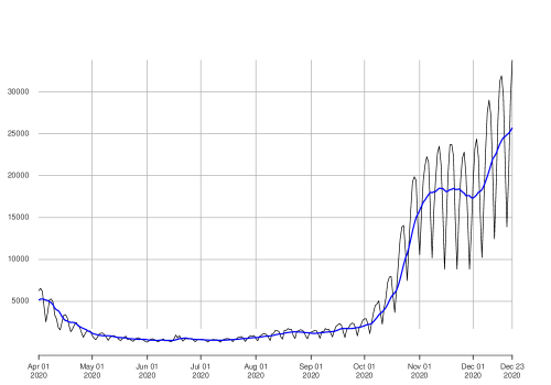
Figure 1: Daily numbers of reported COVID-19-cases, denoted by $\mbox{RKI}_{t}$, in black. A moving average over seven days of $\mbox{RKI}_{t}$ is given in blue.

When considering daily COVID-19-cases it is important to carefully distinguish for individuals the time $t$ at which an SARS-CoV-2-infection took place, the time at which the case was first reported to the (local) health authorities (if it was laboratory confirmed at all) and the time at which the case finally was reported to RKI.
For the investigations in this paper we typically consider times $t$ at which an infection with SARS-CoV-2 takes place. It is most likely that the difference of the time of infection of a case, which in the end will be reported, and the time of reporting follows a distribution over a couple of days. On average, we assume a time shift of $\tau=7$ days, which seems to be reasonable. $\tau$ consists of the number of days (approximately $4$) between a SARS-CoV-2 infection took place and the onset of symptoms plus the time that elapses (after onset of symptoms) until a PCR-test is carried out and a (positive) result becomes known (approximately another $2$ days) plus the time (approximately another day) that elapses until the case is first reported to the health authorities. It is important to know that in Germany it is mandatory that for a person for whom a proof of the pathogen SARS-CoV-2  is obtained (mostly by a PCR-test), a report has to be transmitted to the local health department within 24 hours. After this first reporting time to the health authorities the reporting chain is continued via the responsible state health authorities to the Robert Koch Institute, which will take further days.
For this paper the relevant times are the infection time and the time of the first reporting. We denote by $\mbox{RKI}_{s}$ the number of COVID-19-cases first reported at time $s$ to the health authorities. Then, roughly speaking the number of infections at time $t$, which in the end will be reported, and $\mbox{RKI}_{t+\tau}$ are related to each other.
Figure 1 displays the daily data $\mbox{RKI}_{t}$ for the second, third and fourth quarter of 2020 together with a moving average smoothing over $7$ days. Averaging over $7$ days seems to be appropriate since a very strong periodic behavior of $\mbox{RKI}_{t}$ over the week is observed. The reason for this most likely lies in the fact that the reporting chain between weekdays and weekends is substantially different. We argued that it is important to estimate not only the expectation but also the dispersion or equivalently the variance of the individual reproduction number $R$, for example in order to assess whether or not this quantity changes over time. To do so we present a setup of assumptions under which we are able to give reasonable estimates of the variance (or dispersion) of $R$. To this end it appears to be necessary to rely on COVID-19-data on district (Landkreis) level in Germany.

As a result it will be seen that the parameters of the distribution of $R$ indeed have changed over time and that dispersion (even over-dispersion) is rather relevant. We will make the implication of this clear and we also report upon simulation results which describe the changes in the behavior of the development of the pandemic if the rather relevant super-spreading events are (to some extend) quickly discovered by the health authorities with the result that a substantial part of the secondary infected individuals in such a super-spreading event can promptly be isolated.
There exist already numerous papers in the literature which investigate the effects of social distancing or contact bans and also of cluster tracing within a variety of models. Dehningetal2020a used MCMC-sampling in a SIR-model and obtained that already in case of mild social distancing a substantial reduction of the spreading rate is achieved. Contrerasetal2020 describe that contact tracing is very effective in stabilizing the number of infections (i.e. the observed number of newly infected individuals approaches a constant value), while inefficient contact tracing leads to an approximately exponential growth of the number of infections. Moreover, the paper emphasizes that a combination of symptom-based testing together with effective contact tracing appears to be most effective. Additionally Lindenetal2020 describe clearly that a break-down of a TTI-strategy (Test-Trace-Isolate) will lead to an increasing number of not-reported COVID-19-cases and therefore accelerates the spread of the virus.

The paper is organized as follows. In the next section we describe our modeling and state the main assumptions used for our results. Section 3 presents the proposed estimators of the mean and of the variance of the individual reproduction number taking into account under-reporting and the time behavior of the infection and of the reporting chain. Section 4 introduces Bootstrap-based confidence intervals for $R_{0}$. Section 5 examines the fit of the distributional assumptions made, presents estimators describing the development of the COVID-19 pandemic in Germany, and studies effectiveness of cluster tracing.

2 Modeling and Assumptions

As already mentioned, the Negative Binomial distribution has been suggested in the literature as an appropriate model to describe the randomness of the reproduction number $R$. The Negative Binomial distribution with parameters $p\in(0,1)$ and $r\in\mathbb{N}$ is well-known in statistics for modeling the number of failures in a sequence of independent Bernoulli($p$)-trials until the $r$-th success occurs. It has been extended to parameters $p\in(0,1)$ and $r\in(0,\infty)$ (we use the abbreviation $\mathcal{NB}(p,r)$) via a consideration of a classical Poisson-distribution with random parameter $\lambda$ distributed according to a specific Gamma-distribution. To be precise a random variable $R$ possesses a (generalized) Negative Binomial distribution $\mathcal{NB}(p,r)$, if and only if

$$P_{p,r}(R=k)=\int_{0}^{\infty}e^{-\lambda}\frac{\lambda^{k}}{k!}\,f_{r,\frac{p}{1-p}}(\lambda)\,d\lambda,\ \ k\in\mathbb{N}_{0},$$ (1)

with

$$f_{r,\frac{p}{1-p}}(\lambda)=\frac{1}{\Gamma(r)}\big{(}\frac{p}{1-p}\big{)}^{r}\lambda^{r-1}e^{-\lambda\frac{p}{1-p}},$$

the density of a Gamma-Distribution with parameters $r\in(0,\infty)$, $p/(1-p)\in(0,\infty)$ and $\Gamma(r)=\int_{0}^{1}x^{r-1}e^{-x}dx$ the Gamma function.

The Negative Binomial distribution as a generalized Poisson distribution allows for a more flexible modeling of rare events with different expectation and variance. For $R\sim\mathcal{NB}(p,r)$ we have

$$\mbox{E}(R)=\frac{r\,(1-p)}{p}\ \ \text{\rm and }\ \ \mbox{Var}(R)=\frac{r\,(1-p)}{p^{2}}.$$ (2)

Typically the expectation $\mbox{E}(R)$ is denoted by $R_{0}$. The Negative Binomial distribution possesses a coefficient of variation $\mbox{CV}(R)=\mbox{Var}(R)/\mbox{E}(R)=1/p$, and allows for modeling the distribution of the reproduction number $R$ with dispersion.
The dispersion parameter $\kappa$ is defined through

$$\mbox{Var}(R)=R_{0}\cdot\Big{(}1+\frac{R_{0}}{\kappa}\Big{)},$$ (3)

which leads to $\kappa=r$ (cf. LloydSmithetal2005). The dispersion parameter $\kappa$ and the coefficient of variation both are widely used to quantify the size of the variance given the expectation of a random variable. For fixed $\mbox{E}(R)=R_{0}$ we have that the smaller $r$ the larger is the variance of the reproduction number $R$. To see that $\kappa$ and CV behave rather the same let us assume two sets of parameters $(p,r)$ and $(\widetilde{p},\widetilde{r})$ of Negative Binomial distributions describing the random behavior of two reproduction numbers $R$ and $\widetilde{R}$ (with dispersion parameters $\kappa$ and $\widetilde{\kappa}$). If we fix $\mbox{E}R=\mbox{E}\widetilde{R}=R_{0}$ then

$$\frac{\mbox{CV}(\widetilde{R})}{\mbox{CV}(R)}=\frac{\kappa\cdot(R_{0}+\widetilde{\kappa})}{\widetilde{\kappa}\cdot(R_{0}+\kappa)},$$ (4)

which is a decreasing function in $\widetilde{\kappa}$.

For Negative Binomial distributions it is known that $r\to\infty$ and $p\to 1$, such that $r(1-p)\to\lambda\in(0,\infty)$, leads to a classical Poisson($\lambda$)-limit, while for $r=1$ the Negative Binomial distribution coincides with the geometric distribution with parameter $p$.

We will model the number of secondary infections caused by an individual COVID-19-case with infection time (day) $t$, i.e., the reproduction number $R_{t}$ at time $t$, via a $\mathcal{NB}(p_{t},r_{t}$)-distribution. If we further denote the number of newly infected cases at time $t$ by $N_{t}$, we then are faced with a total of

$$\sum_{i=1}^{N_{t}}S_{i,t},$$ (5)

secondary infections in the future. Here $S_{1,t},S_{2,t},\ldots$ denote i.i.d. random variables distributed according to $\mathcal{NB}(p_{t},r_{t}$). It should be noted that the random variables $S_{i,t},i=1,2,\ldots,$ are i.i.d. copies of $R_{t}$. In order to avoid confusion we decided to use the notation $R_{t}$ for the generic reproduction number, while we label the random secondary infections from a single infected individual by $S_{i,t}$.

For several reasons not all of these future cases will be reported to the German health authorities and subsequently will not show up in the RKI-statistics of newly laboratory-confirmed COVID-19-cases. One major, but not the only reason for this under-reporting is that a substantial number of SARS-CoV-2-infections are asymptomatic. The studies Buitrago2020 and OranTopol2020 report that percentages of asymptomatic cases vary between 20% to 45%. These values coincide with results from a study in the community of Kupferzell (Germany), where a percentage of asymptomatic cases of 24.5% has been observed, cf. Santosetal2020.
Although it seems difficult to assess the exact rate of under-reporting, this rate is of course a relevant quantity when investigating the development of the pandemic. Some studies state rates of not reported cases up to 80%. See for example Streecketal2020, where a 5-fold higher number of infections than the number of officially reported cases for a specific community in Germany with a super-spreading event is reported or the already cited study in Kupferzell (Santosetal2020), where is was observed that six times more adults than reported have been infected, which is a rate of under-reporting of 80% or even higher. This coincides with statements made by the RKI, that the number of infected individuals approximately is 4-6 times higher than the number of reported cases. Besides this, the RKI stated that there is no evidence for a substantial change of this factor over the last months. Finally, Rahmandadetal2020, in a study across 86 nations, found out that under-reporting varies substantially over countries. For Germany, Rahmandadetal2020 estimated a ratio of actual to reported cases of about 6 to 7.
In this paper we denote the proportion of COVID-19-cases reported to the German health authorities by $p_{0,t}$, and allow this rate to vary (slowly) with time. A value of $p_{0,t}\approx 0.2$ seems realistic in the light of the studies cited.
From a number of $N_{t}$ newly infected individuals at time $t$ we therefore will see within the statistics of RKI only a binomial thinned selection of $N_{t}$, which we denote by $N_{t}^{\prime}$. According to our assumption of a reporting rate of $p_{0,t}$ and because of a not small number of cases it is reasonable to assume that, approximately,

$$\frac{N_{t}^{\prime}}{N_{t}}\approx p_{0,t}.$$ (6)

It is worth mentioning that the number of reported cases $N_{t}^{\prime}$ out of infections happened at time $t$ do not show up within the RKI-statistics neither at time $t$ nor at a single time point in the future. Rather, occurrence in the RKI-statistics will spread over a span of days.

This further means that from the total number $\sum_{i=1}^{N_{t}}S_{i,t}$ of secondary infections caused by $N_{t}$ primary infections we only observe $\sum_{i=1}^{N_{t}}\widetilde{S}_{i,t}$ laboratory-confirmed cases with the statistics of RKI, where $\widetilde{S}_{i,t}$ possesses a Binomial-distribution with parameters $S_{i,t}$ and $p_{0,t}$. Equivalently, the number of reported SARS-CoV-2 secondary infections out of a cohort of $N_{t}$ primary infected individuals can be written as

$$\sum_{i=1}^{N_{t}}\sum_{j=1}^{S_{i,t}}Z_{i,j},$$ (7)

where $(Z_{i,j},i,j\in\mathbb{N})$ is a family of i.i.d. Bernoulli($p_{0,t}$)-distributed random variables. Success, i.e. $Z_{i,j}=1$, means that a secondary infected individual gets a positive COVID-19-test at some day in the future. As stated above it is of course not realistic to assume that all $\sum_{i=1}^{N_{t}}\sum_{j=1}^{S_{i,t}}Z_{i,j}$ cases will show up in the RKI-statistics at one single day. Rather occurrence of these cases in the RKI-statistics will spread over a span of some days.

Before further elaborating on this point let us take a look at the distribution of the total numbers of secondary infections $\sum_{i=1}^{N_{t}}S_{i,t}$ and reported secondary infections $\sum_{i=1}^{N_{t}}\widetilde{S}_{i,t}$. Since it is known that the Negative Binomial distribution is additive, we immediately obtain, assuming independence of the single cases, that $\sum_{i=1}^{N_{t}}S_{i,t}\sim\mathcal{NB}(p_{t},N_{t}\cdot r_{t})$. Moreover, $\widetilde{S}_{i,t}$ is a Binomial-thinning of $S_{i,t}$. The property that Binomial-thinning changes the parameter but not the family of Poisson-distributions carries over to the family of Negative Binomial distributions, cf. Lemma 1 of the Appendix. This means that we end up with

$$\widetilde{S}_{i,t}\sim\mathcal{NB}(q_{t},r_{t}),\ \ i=1,2,\ldots,$$ (8)

with

$$q_{t}=\frac{p_{t}}{p_{0,t}+p_{t}-p_{0,t}\cdot p_{t}}.$$ (9)

The parameter $q_{t}$ depends on the hardly known percentage $p_{0,t}$ of SARS-CoV-2-infections reported to the health authorities. Furthermore,

$$\sum_{i=1}^{N_{t}}\widetilde{S}_{i,t}\sim\mathcal{NB}(q_{t},N_{t}\cdot r_{t}).$$ (10)

So far we focused on time points $t$ at which SARS-CoV-2-infections take place. We already discussed in the introduction that these time points $t$ should not be confused with the time points at which SARS-CoV-2-infections are first reported to the health authorities (recall that we denoted the number of COVID-19-cases first reported at time point $t$ to the health authorities by $\rm{RKI}_{t}$). We argued that there is a (random) time shift between these two time points with a likely mean of $\tau=7$.

So as not to make things too complicated and still take time shifts as well as random fluctuations of reporting delays over a span of days into account, we make the following two assumptions

$$\sum_{s=0}^{6}N_{t-s}^{\prime}\approx\sum_{s=0}^{6}\rm{RKI}_{t+\tau-s}.$$ (11)

and

$$\sum_{s=0}^{6}N_{t-s}^{\prime}\approx\sum_{s=0}^{6}\sum_{i=1}^{N_{t-4-s}}\widetilde{S}_{i,t-4-s}.$$ (12)

The first assumption means that newly infected cases, which are of a type that will be reported in the future, summed up over a week approximately will occur in the RKI-statistics also within a week but shifted by $\tau$ days to the future, while the second assumption is a relaxation of $N_{t}^{\prime}\approx\sum_{i=1}^{N_{t-4}}\widetilde{S}_{i,t-4}$. The latter assumption would mean that secondary infections occur with a fixed time delay of $4$ days to the primary infection. Instead of such a strict assumption (12) means that the two quantities are roughly the same if they are summed up over a week. Here the number $4$ can be viewed as generation time of the virus.

3 Estimation of Parameters of the Distribution of the Reproduction Number

Based on the assumptions made in the previous section it follows that the smoothed estimate of the mean of the reproduction number published on a daily basis by RKI, and denoted by $\widehat{R}_{0,t}^{7}$ fulfills

$$\widehat{R}_{0,t}^{7}:=\frac{\sum_{s=0}^{6}\rm{RKI}_{t-s}}{\sum_{s=0}^{6}\rm{RKI}_{t-4-s}}\approx\frac{\sum_{s=0}^{6}N_{i,t-\tau-s}^{\prime}}{\sum_{s=0}^{6}N_{t-4-\tau-s}^{\prime}}\approx\frac{\sum_{s=0}^{6}\sum_{i=1}^{N_{t-4-\tau-s}}\widetilde{S}_{i,t-4-\tau-s}}{\sum_{s=0}^{6}N_{t-4-\tau-s}^{\prime}},$$ (13)

cf. (11) and (12). It is often noted that $\widehat{R}_{0,t}^{7}$ reflects the reproduction behavior approximately $14$ days ago. To understand this, notice that we need two generations of SARS-CoV-2-infected individuals in order to be able to compute reproduction numbers. Since the generation time of SARS-CoV-2 is approximately $4$ days and since the proposed computation of the reproduction number uses a left-sided smoothing over $7$ days (cf. (13)), which leads to a time-shift of $3$, a reasonable reproduction number can only be calculated with a delay of $4+3$ days after primary infections have taken place. Because $\widehat{R}_{0,t}^{7}$ in (13) is computed on the basis of reported case numbers we have to face on top the aforementioned general reporting delay of $\tau$, for which $\tau=7$ seems realistic. In total for $\widehat{R}_{0,t}^{7}$ we end up with a delay of about $14$ days in describing the reproduction behavior of SARS-CoV-2.

From (10) we have that the distribution of the numerator $\sum_{s=0}^{6}\sum_{i=1}^{N_{t-4-\tau-s}}\widetilde{S}_{i,t-4-\tau-s}$, given the numbers $N^{\prime}_{t-4-\tau-s},s=0,\ldots,6,$ approximately is (assume that $q_{t}$ and $r_{t}$ only vary slowly over time and therefore $q_{t-4-\tau-s}\approx q_{t-\tau-7}$ and $r_{t-4-\tau-s}\approx r_{t-\tau-7},s=0,\ldots,6$)

$$\mathcal{NB}(q_{t-\tau-7},r_{t-\tau-7}\cdot\sum_{s=0}^{6}N_{t-\tau-4-s}),$$ (14)

with (conditional on $\sum_{s=0}^{6}N_{t-\tau-4-s}$) expectation

$$\sum_{s=0}^{6}N_{t-\tau-4-s}\cdot\frac{r_{t-\tau-7}\cdot(1-q_{t-\tau-7})}{q_{t-\tau-7}}.$$ (15)

Using the further approximation from (6) this leads to the following value that is estimated by $\widehat{R}_{0,t}^{7}$

$$\frac{\sum_{s=0}^{6}N_{t-4-\tau-s}}{\sum_{s=0}^{6}N_{t-4-\tau-s}^{\prime}}\cdot\frac{r_{t-\tau-7}\,(1-q_{t-\tau-7})}{q_{t-\tau-7}}=\frac{1}{p_{0,t-\tau-7}}\cdot\frac{r_{t-\tau-7}\,(1-q_{t-\tau-7})}{q_{t-\tau-7}}.$$ (16)

Fortunately, we obtain by simple algebra and using (9), that

$$\frac{1}{p_{0,t-\tau-7}}\cdot\frac{r_{t-\tau-7}\,(1-q_{t-\tau-7})}{q_{t-\tau-7}}=\frac{r_{t-\tau-7}\,(1-p_{t-\tau-7})}{p_{t-\tau-7}},$$ (17)

which is the expectation $R_{0,t-\tau-7}$ of the reproduction number $R_{t-\tau-7}$ we are interested in.

In order to be able to estimate both parameters $r$ and $p$ of a Negative Binomial fit to the distribution of the reproduction number $R$ we further need an estimator of $\mbox{Var}(R)$. For this we need somehow replicates of realizations of $R$, which we will obtain from reported COVID-19-cases on district level from Germany. In total, Germany is divided into about $401$ districts with population numbers ranging from $34,193$ to $3,669,491$. For each district RKI provides daily COVID-19-cases along the same guidelines as for Germany as a whole. As before we denote the number of newly infected (not necessarily reported!) COVID-19-cases by $N_{t,\ell}$, where $t$ counts the day (time) and $\ell=1,\ldots,L=401$ denotes the number of the district. For a single primary infected individual we assume that the total number of secondary infected persons possesses a $\mathcal{NB}(p_{t},r_{t})$-distribution, which does not depend on the district. The total number of secondary infections caused by $N_{t,\ell}$ primary infected individuals then follows a $\mathcal{NB}(p_{t},N_{t,\ell}\cdot r_{t})$-distribution. Following the arguments in Section 2 we obtain that the total number of (in the end) reported SARS-CoV-2- secondary infections out of a number of $N_{t,\ell}$ primary infections in district $\ell$, which we denote by $N_{t,\ell}^{\prime}$, is distributed according to $\mathcal{NB}(q_{t},N_{t,\ell}\cdot r_{t})$, cf. (14) and (13). Note that if there is evidence that the infection rates of some districts differs highly from the infection rates of the others then a subset selection might be preferable.

In order to relate the number of daily first reported cases $\rm{RKI}_{t,\ell}$ within district $\ell$ with the total number of secondary infections $N_{t,\ell}^{\prime}$, for which the reporting is spread over some of days, we assume in accordance with (11) and (12) for each district $\ell=1,2,\ldots,L$

$$\sum_{s=0}^{6}N_{t-s,\ell}^{\prime}\approx\sum_{s=0}^{6}\rm{RKI}_{t+\tau-s,\ell},$$ (18)

and

$$\sum_{s=0}^{6}N_{t-s,\ell}^{\prime}\approx\sum_{s=0}^{6}\sum_{i=1}^{N_{t-4-s,\ell}}\widetilde{S}_{i,t-4-s}.$$ (19)

Along the same lines as above (cf. (13)) the standard 7-days reproduction number of RKI, i.e., for each $\ell=1,2,\ldots,L$

$$\widehat{R}_{0,t,\ell}^{7}:=\frac{\sum_{s=0}^{6}\rm{RKI}_{t-s,\ell}}{\sum_{s=0}^{6}\rm{RKI}_{t-4-s,\ell}}$$ (20)

provides an estimator of $\mbox{E}(R)=r_{t-\tau-7}\cdot\big{(}1-p_{t-\tau-7}\big{)}/p_{t-\tau-7}$, which by our assumptions does not depend on $\ell$.

Averaging estimator (20) over the districts and taking the heterogeneous variance into account, see (22), exactly leads to the 7-days smoothed RKI-estimator $\widehat{R}_{0,t}^{7}$ of the reproduction number based on reported COVID-19-cases all over Germany (see Figure  2).

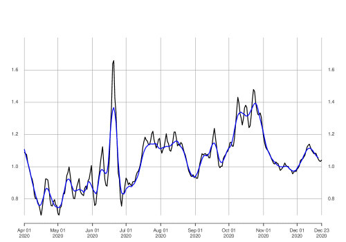
Figure 2: The black line shows the 7-days smoothed RKI-estimator $\widehat{R}_{0,t}^{7}$. A moving average of $\widehat{R}_{0,t}^{7}$ of order $7$ is given in blue.

Our main focus, when turning to reported COVID-19-cases on district level, is to obtain an estimator of the variance $\mbox{Var}(R_{t-\tau-7})=r_{t-\tau-7}\cdot\big{(}1-p_{t-\tau-7}\big{)}/p_{t-\tau-7}^{2}$. Because of the approximation of the distribution of the numerator of $\widehat{R}_{0,t,\ell}^{7}$ by a $\mathcal{NB}(q_{t-\tau-7},r_{t-\tau-7}\cdot\sum_{s=0}^{6}N_{t-\tau-4-s,\ell})$-distribution together with the approximation

$$\frac{\sum_{s=}^{6}N_{t-\tau-4-s}^{\prime}}{\sum_{s=0}^{6}N_{t-\tau-4-s}}\approx p_{0,t-\tau-7},$$ (21)

cf. (6) and also (16), we obtain for given $\sum_{s=0}^{6}N_{t-\tau-4-s}=\sum_{s=0}^{6}\rm{RKI}_{t-4-s,\ell}/p_{0,t-\tau-7}$, i.e., the denominator is considered fix,

$$\mbox{Var}(\widehat{R}_{0,t,\ell}^{7})\approx\frac{1}{\sum_{s=0}^{6}\rm{RKI}_{t-4-s,\ell}\,p_{0,t-\tau-7}}r_{t-\tau-7}(1-q_{t-\tau-7})/q_{t-\tau-7}^{2}.$$ (22)

This means, the variance is heterogeneous among the districts with a factor $1/\sum_{s=0}^{6}\rm{RKI}_{t-4-s,\ell}$. Taking this into account leads to the estimator (23), which is an estimator for $\mbox{Var}(\widetilde{S}_{i,t-\tau-7})/p_{0,t-\tau-7}$, i.e., the variance of the number of reported SARS-CoV-2-secondary infection cases from a single infected individual scaled by $1/p_{0,t-\tau-7}$.

$$\widehat{\mbox{Var}(\widetilde{S}_{t-\tau-7})}:=\frac{1}{L}\sum_{\ell=1}^{L}\,\sum_{s=0}^{6}\rm{RKI}_{t-4-s,\ell}\left(\widehat{R}_{0,t,\ell}^{7}-\widehat{R}_{0,t}^{7}\right)^{2}.$$ (23)

Note that not necessarily an independence assumption across districts is required in order for (23) to be a consistent estimator. Only consistency of sample moments is required, which, for instance, can be achieved under some rather weak dependence assumptions. This means that neighboring districts may be dependent but districts which are far apart from each other should behave nearly independent.

Since the distribution of $\widetilde{S}_{i,t}$ is $\mathcal{NB}(q_{t},r_{t})$ we obtain

$$\frac{1}{p_{0,t}}\cdot\mbox{Var}(\widetilde{S}_{i,t}) =\frac{r_{t}\cdot(1-q_{t})}{p_{0,t}q_{t}^{2}}$$

$$=\frac{r_{t}\cdot(1-p_{t})}{p_{t}^{2}}\cdot(p_{0,t}+p_{t}-p_{0,t}p_{t})$$

$$=\mbox{Var}(R_{t})\cdot(p_{0,t}+p_{t}-p_{0,t}p_{t}),$$ (24)

that is, for $p_{t}>0$,

$$\mbox{Var}(R_{t})=\frac{1}{(p_{0,t}+p_{t}-p_{0,t}p_{t})}\,\cdot\frac{1}{p_{0,t}}\mbox{Var}(\widetilde{S}_{i,t}).$$ (25)

As it is seen, and in contrast to the expectation (cf. (17)), the variance of the reproduction number based on COVID-19-cases reported to the health authorities depends on the unknown reporting rate $p_{0,t}$. Since the reporting rate $p_{0,t}$ cannot be estimated from reported data we only can calculate variance estimators for a variety of assumed reporting rates $p_{0,t}$ (see Figure 3). Based on estimators $\widehat{\mbox{E}R_{t-14}}:=\widehat{R}_{0,t}^{7}$, cf. (13), with $\tau=7$, $\widehat{\mbox{Var}(\widetilde{S}_{t-14})}$ as given in (23) and because of (25) together with explicit expressions of expectation and variance of the Negative Binomial distribution $\mathcal{NB}(p_{t-14},r_{t-14})$ assumed for $R_{t-14}$, we finally are led to the following estimators $\widehat{p}_{t-14}$ and $\widehat{r}_{t-14}$ for any fixed value of $p_{0,t-14}$ and the choice of $\tau=7$.

$$\widehat{p}_{t-14}=\frac{\widehat{R}_{0,t}^{7}\cdot p_{0,t-14}}{\widehat{\mbox{Var}(\widetilde{S}_{t-14})}-\widehat{R}_{0,t}^{7}\cdot(1-p_{0,t-14})}\ \ \text{and}\ \ \widehat{r}_{t-14}=\frac{\widehat{R}_{0,t}^{7}\cdot\widehat{p}_{t-14}}{1-\widehat{p}_{t-14}}\,.$$ (26)

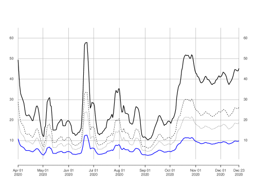
Figure 3: The estimates of the variances $\mbox{Var}(\widetilde{S}_{t-\tau-7})/p_{0,t-\tau-7}$ (in blue) and $\mbox{Var}(R_{t-\tau-7})$ for $p_{0}=0.2$ (black solid line), $p_{0}=0.35$ (black dashed line), $p_{0}=0.5$ (black dotted line).

4 Bootstrap Confidence Intervals

Besides estimating the mean and the variance of the individual reproduction number $R_{t}$ as well as the parameters of the corresponding Negative Binomial distribution, it is important to construct confidence intervals for the unknown mean $R_{0,t}$. According to our previous discussion, the numerator of the estimator $\widehat{R}_{0,t}^{7}$ approximately satisfies for $\tau=7$

$$\sum_{s=0}^{6}RKI_{t-s}\sim\mathcal{NB}\big{(}q_{t-14},r_{t-14}\cdot\sum_{s=0}^{6}RKI_{t-s-4}/p_{0,t-14}\big{)};$$ (27)

see also the discussion before and after equation (21) for the same property for observations obtained at the district level. Recall that this distribution depends on the unknown under-reporting rate $p_{0,t-14}$. Based on expression (27) the following parametric bootstrap procedure can be proposed for constructing a confidence interval for the mean $R_{0,t-14}$ of the individual reproduction number.

Bootstrap Algorithm, Confidence Intervals for $R_{0,t-14}$:

1. Step 1:   For $p_{0,t-14}$ given and estimates $\widehat{q}_{t-14}$ and $\widehat{r}_{t-14}$, we generate for $t=15,16,\ldots,n$, pseudo random variables $(\sum_{s=0}^{6}RKI_{t-s})^{\ast}$ distributed as

   $$\big{(}\sum_{s=0}^{6}RKI_{t-s}\big{)}^{\ast}\sim\mathcal{NB}\big{(}\widehat{q}_{t-14},\widehat{r}_{t-14}\cdot\big{(}\sum_{s=0}^{6}RKI_{t-s-4}\big{)}^{\ast}\big{/}p_{0,t-14}\big{)},$$ (28)

   using the starting values

   $$\big{(}\sum_{s=0}^{6}RKI_{t-s-4}\big{)}^{\ast}=\sum_{s=0}^{6}RKI_{t-s-4},$$

   for $t=15,16,17$ and $18$.

2. Step 1:   Calculate for $t=15,16,\ldots,n$ the pseudo estimator

   $$\widehat{R}^{\ast}_{t}=\frac{\big{(}\sum_{s=0}^{6}RKI_{t-s}\big{)}^{\ast}}{\big{(}\sum_{s=0}^{6}RKI_{t-s-4}\big{)}^{\ast}}.$$

3. Step 3:  Repeat Step 1 and Step 2 a large number of times, say $B$ times, and denote by

   $$\widehat{R}^{\ast}_{t,1},\ \widehat{R}^{\ast}_{t,2},\ldots,\ \widehat{R}^{\ast}_{t,B}$$

   the pseudo-random variables obtained for $t\in\{15,16,\ldots,n\}$.

4. Step 4:  For a desired $1-\alpha$ confidence level, let $Q_{1}=[B*\alpha/2]$ and $Q_{2}=[B*(1-\alpha/2)]$. A $(1-\alpha)100\%$ confidence interval for $R_{0,t}$ is then given by

   $$\big{[}\widehat{R}^{\ast}_{t,(Q_{1})},\ \widehat{R}^{\ast}_{t,(Q_{2})}\big{]},$$

   where $\widehat{R}^{\ast}_{t,(1)},\widehat{R}^{\ast}_{t,(2)},\ldots,\widehat{R}^{\ast}_{t,(B)}$ denotes the ordered values of the random sample $R_{t,i}^{\ast}$, $i=1,2,\ldots,B$, generated in Step 3.

Notice that the above algorithm imitates also the dependence in generating the random sums $(\sum_{s=0}^{6}RKI_{t-s})^{\ast}$ by using the time dependent parameters $\widehat{p}_{t-14}$ and $\widehat{r}_{t-14}$ as well as the (by four time units) lagged sum $(\sum_{s=0}^{6}RKI_{t-s-4})^{\ast}$. Since we need $\widehat{p}_{t-14}$ and $\widehat{r}_{t-14}$, to generate $(\sum_{s=0}^{6}RKI_{t-s})^{\ast}$, our bootstrap algorithm starts for $t=15$ and needs starting values like those given in Step 1.

A simplified version of the proposed bootstrap algorithm can be applied when interest is focused in the construction of a confidence interval for a particular time point $t$ only. In this case $(\sum_{s=1}^{6}RKI_{t-s-4})^{\ast}$ in equation (28) can be treated as fixed and replaced by the observed sum $\sum_{s=0}^{6}RKI_{t-s-4}$. Notice that in this case, the bootstrap algorithm essentially estimates via Monte Carlo the percentage points of the Negative Binomial distribution, $\mathcal{NB}\big{(}\widehat{q}_{t-14},\widehat{r}_{t-14}\cdot\big{(}\sum_{s=0}^{6}RKI_{t-s-4}\big{)}\big{/}p_{0,t-14}\big{)}$. Furthermore, also in this case and by construction,

$$E^{\ast}(R^{\ast}_{t}) =\frac{1}{p_{0,t-14}}\cdot\frac{\widehat{r}_{t-14}\big{(}1-\widehat{q}_{t-14}\big{)}}{\widehat{q}_{t-14}}=\frac{\widehat{r}_{t-14}\big{(}1-\widehat{p}_{t-14}\big{)}}{\widehat{p}_{t-14}}$$

see also (17), which is the expected value $R_{0,t-14}$ of the individual reproduction number $R_{t-14}$ and the parameter which the estimator $\widehat{R}_{0,t}^{7}$ actually estimates. Thus like the estimator $\widehat{R}_{0,t}$, the bootstrap delivers a confidence interval for $R_{0,t-14}$.

Figure 4 shows estimators $\widehat{R}_{0,t}^{7}$ obtained from COVID-19-cases reported to RKI in Germany together with the corresponding $95\%$ pointwise confidence intervals constructed using the bootstrap algorithm proposed in this section.

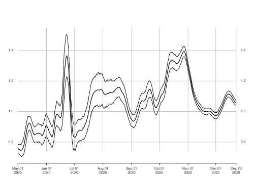
Figure 4: Estimates $\widehat{R}_{0,t}^{7}$ and the $95\%$ pointwise confidence intervals for different reporting rates $p_{0}=0.2$ (solid) and $p_{0}=0.5$ (dotted).

5 Applications

5.1 Validating the Negative Binomial Hypothesis

We first investigate the suitability of the assumed Negative Binomial distribution for describing the random behavior of the individual reproduction number using the number of infections reported by RKI. Toward this end and as for estimating the variance, we focus on reported COVID-19-cases on district level, i.e., on the observations $RKI_{t,\ell}$. This allows for getting replicates of the random variable of interest and, therefore, for testing the hypothesis that the individual reproduction number follows a Negative Binomial distribution. Recall that in our discussion in Section 3, it was assumed that the sum of reported cases over the time points $t,t-1,\ldots,t-6$ in district $\ell$, that is, $\sum_{s=0}^{6}RKI_{t-s,\ell}$, satisfies $(\tau=7),$

$$\sum_{s=0}^{6}RKI_{t-s,\ell}\sim\mathcal{NB}(q_{t-14},r_{t-14}\cdot\sum_{s=0}^{6}N_{t-11-s,\ell}).$$

Assuming that $p_{0,t}$ remains almost constant in the range of $\tau$ days we get using (6) and (11) that

$$\sum_{s=0}^{6}N_{t-11-s,\ell}\approx p_{0,t-14}\sum_{s=0}^{6}N^{\prime}_{t-11-s,\ell}\approx p_{0,t-14}\sum_{s=0}^{6}RKI_{t-4-s,\ell}.$$

That is, in terms of the observed RKI data, the assumption we have to test translates to

$$\sum_{s=0}^{6}RKI_{t-s,\ell}\sim\mathcal{NB}\big{(}q_{t-14},\ \frac{1}{p_{0,t-14}}\cdot r_{t-14}\cdot\sum_{s=0}^{6}RKI_{t-4-s,\ell}\big{)}.$$ (29)

In order to select from the existing data appropriate samples for testing the above assumption, we proceed as follows. We first select all districts for which the average of reported cases at time points $t-4,t-5,\ldots,t-11$ is approximately the same. Practically, this means that we consider districts for which

$$\frac{1}{7}\sum_{s=0}^{6}RKI_{t-4-s,\ell}\in[15,25].$$ (30)

We have experienced that chosen a number of average daily infections at district level outside the above interval, leads to the selection of a relatively small number of districts, that is to a small sample size. Let $L_{t,S}$ be the total number of districts at time point $t$ satisfying condition (30) and let $\{1,2,\ldots,L_{t,S}\}$ be the corresponding set of districts. From the total number of time points $t$ available, we further only consider those time points, for which $L_{t,S}\geq 75$. This ensures that a sufficiently large number of districts is available for testing the hypothesis of interest. After applying this selection procedure to the $RKI_{t,\ell}$ data, we end up with a total of $T=45$ data points $t$ for which the corresponding condition (30) and $L_{t,S}\geq 75$ is satisfied.

The problem of testing the goodness-of-fit of a Negative Binomial distribution $\mathcal{NB}(p,r)$ when both parameters $p$ and $r$ are unknown, has been considered by some authors in the literature; see Meintanis2005 and Bestetal2009. Meintanis2005 proposed a test based on the comparison of the empirical probability generating function with that of the Negative Binomial distribution with estimated parameters. Bestetal2009 considered tests based on the comparison of third and fourth order moments. In the following we focus on the test proposed by Meintanis2005 but we also report results for the test proposed by Bestetal2009.

The test statistic proposed by Meintanis2005 with suggested parameter $a=5$, applied to the selected RKI data, $Y_{t,\ell}=\sum_{s=0}^{6}RKI_{t-s,\ell},\ell\in\{1,2,\ldots,L_{t,S}\}$, is given by

$$T_{t,n} =\frac{1}{L_{t,S}}\Big{[}\overline{Y}^{2}_{L_{t,S}}\sum_{j,k=1}^{L_{t,S}}I(Y^{+}_{j,k}+5)-2\overline{Y}_{L_{t,S}}\sum_{j,k=1}^{L_{t,S}}Y_{t,j}\Big{\{}(1+\widehat{\rho}_{L_{t,S}})I(Y^{+}_{j,k}+4)-\widehat{\rho}_{L_{t,S}}I(Y^{+}_{j,k}+5)\Big{\}}$$

$$\ \ \ \ +\sum_{j,k=1}^{L_{t,S}}Y_{t,j}\cdot Y_{t,k}\Big{\{}(1+\widehat{\rho}_{L_{t,S}})^{2}I(Y^{+}_{j,k}+3)+\widehat{\rho}_{L_{t,S}}I(Y^{+}_{j,k}+5)$$

$$\ \ \ \ -2\widehat{\rho}_{L_{t,S}}(1+\widehat{\rho}_{L_{t,S}})I(Y^{+}_{j,k}+4)\Big{\}}\Big{]},$$

where $Y^{+}_{j,k}=Y_{t,j}+Y_{t,k}$, $I(\beta)=(1+\beta)^{-1}$ for $\beta>-1$ and

$$\widehat{\rho}_{L_{t,S}}=\Big{(}S^{2}_{L_{t,S}}-\overline{Y}_{L_{t,S}}\Big{)}\Big{/}\overline{Y}_{L{t,S}},$$

with $\overline{Y}_{L_{t,S}}=L_{t,s}^{-1}\sum_{j=1}^{L_{t,S}}Y_{t,j}$ and

$$S^{2}_{L_{t,S}}=L_{t,s}^{-1}\sum_{j=1}^{L_{t,S}}(Y_{t,j}-\overline{Y}_{L_{t,S}})^{2}.$$

To obtain critical values of the $T_{t,n}$ test, a parametric bootstrap procedure is used. More specifically, i.i.d. random samples of length $L_{t,S}$ are generated from a $\mathcal{NB}(\widehat{q}_{t},\widehat{r}_{t})$ distribution, where

$$\widehat{q}_{t}=\frac{\widehat{r}_{t}}{\widehat{r}_{t}+\overline{Y}_{L_{t,S}}}\ \ \mbox{and}\ \ \widehat{r}_{t}=\frac{L_{t,S}^{-1}\sum_{j=1}^{L_{t,S}}Y_{t,j}^{2}}{S^{2}_{L_{t,S}}-\overline{Y}_{L_{t,S}}}.$$

The distribution of the test statistic $T_{t,n}$ under the null is then estimated using the distribution of the same test statistic calculated using the bootstrap pseudo random sample.

Applying the above test to the RKI data sets selected according to the described procedure, the null hypothesis of a Negative Binomial distribution has been rejected at the $5\%$ level in only $8$ out of the $45$ different data sets considered. Notice that qualitatively the same result is obtained, if one uses the test proposed by Bestetal2009. As already mentioned, this test compares the empirical third and fourth moments with those of the Negative Binomial distribution fitted to the data; see the test denoted by $R^{2}/Var(R)$ in page 6 of the cited paper. Applying this test leads to a rejection of the the null hypothesis at the $5\%$ level, in only $2$ out of the $45$ data sets selected. Our testing procedures find, therefore, no evidence against the assumption that the random behavior of the individual reproduction number is governed by a Negative Binomial distribution.

5.2 Empirical Results

In this section we present the estimated parameter of the Negative Binomial distribution obtained for Germany based on the RKI data set by the method described in Section 3. We consider here the time period from April 1, 2020 to December 23, 2020. Furthermore, the moment estimators in Section 3 are based on 401 districts and a left-sided 7-day moving average smoothing is applied to the estimated moments before computing the parameter estimators (26). As mentioned in Section 3, the parameter estimates depend on the unknown reporting rate $p_{0,t}$ and this rate cannot be estimated from the data given. That is why we present results here for three possible reporting rates, i.e., $p_{0,t}\in\{0.2,0.35,0.5\}$. For a given reporting rate, the estimated parameters are presented here as connected lines. However, note that the reporting rate may vary over time and the proposed estimation procedure requires only a locally constant reporting rate, i.e., the estimation at time $t$ requires roughly no substantial changes in the reporting rate for the past three weeks. This means, it is possible to switch over time between the results of different reporting rates, if there is strong believe that the reporting rate changes between different time periods. The estimated parameters $p_{t}$ and $r_{t}$ are given in Figure 5 and  6, respectively. In this time period, $p_{t}$ is in the range of $0.021$ to $0.2$ and $r_{t}$ in range of $0.02$ to $0.25$. The parameters also can be translated into probabilities that an individual case causes a given number of secondary infections over its entire infectious period. For this, we present in Figure 7 the probability that an individual causes no infections, in Figure 8 the probability that an individual causes one to five infections, and in Figure 9 the probability that an individual causes 20 or more infections.

Before discussing the results, first note that over the entire period non-pharmaceutical measures were in place such as mandatory wearing of face masks in public areas, detected cases and contacts were quarantined, etc. This also can be seen in the estimates of the parameter $R_{0}$. Over this time period, the average is $1.036$, and consequently, far less than the reproduction rate without any measures, which is estimated as $3.32$ by Alimohamadi2020 in a meta-study. Over the entire time period a strong overdispersion can be observed irrespective of the reporting rate. Smaller reporting rates lead in general to smaller parameter values for $r_{t}$. Furthermore, in the summer period larger parameter values for $r_{t}$ can be observed than in the fall period. The overdispersion can be displayed well in in probabilities. During the summer period the probability that an individual cases causes no infection is given by $60\%-80\%$ and it rises in the fall period to $80\%-90\%$. Additionally, the probability that an individual case causes 20 or more infections almost doubles from summer to fall and peaks in October with values about $1.5\%-2\%$. In contrast, the probability that an individual case causes one to five infections almost halves from summer to fall with values in summer of about $10\%-20\%$.

Endo2020 estimated the overdispersion parameter $r_{t}$ of the Negative Binomial distribution as $0.1$ with a $95\%$ confidence interval from $0.04$ to $0.2$. Note however, that their considered time period is January and February of 2020. In that time period non-pharmaceutical measures such as obligatory face masks in public areas were not yet in place or less strict than in the time period considered here. Since in our considered time period non-pharmaceutical measures were less strict in Germany during the summer 2020, it seems most reasonable to compare the results obtained in the summer period, June 1, 2020 to October 31, 2020, with the results obtain by Endo2020. In the summer period, $r_{t}$ takes values in the range of $0.025$ to $0.22$ and for a reporting rate of $0.35$, we obtain values in the range of $0.044$ to $0.157$ with a mean value of $0.095$. Hence, the obtained values coincide well with the values obtained in Endo2020.

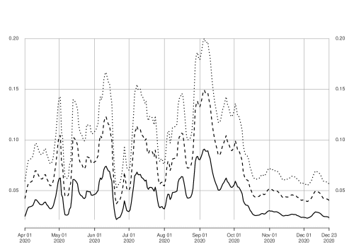
Figure 5: The estimated parameter $p_{t}$ for $p_{0}=0.2$ (black solid line), $p_{0}=0.35$ (black dashed line), $p_{0}=0.5$ (black dotted line).

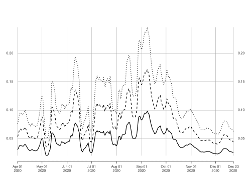
Figure 6: The estimated parameter $r_{t}$ for $p_{0}=0.2$ (black solid line), $p_{0}=0.35$ (black dashed line), $p_{0}=0.5$ (black dotted line).

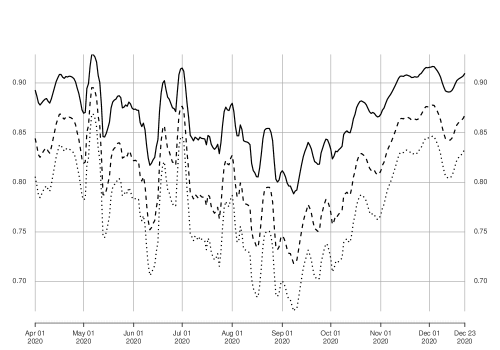
Figure 7: The probability that an individual causes no secondary infection for $p_{0}=0.2$ (black solid line), $p_{0}=0.35$ (black dashed line), $p_{0}=0.5$ (black dotted line)..

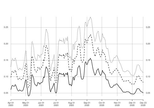
Figure 8: The probability that an individual causes between 1 and 5 secondary infections for $p_{0}=0.2$ (black solid line), $p_{0}=0.35$ (black dashed line), $p_{0}=0.5$ (black dotted line)..

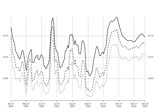
Figure 9: The probability that an individual causes 20 or more secondary infections for $p_{0}=0.2$ (black solid line), $p_{0}=0.35$ (black dashed line), $p_{0}=0.5$ (black dotted line)..

5.3 Simulated Interventions - Cluster Tracing

The estimated parameters can be used to simulate the effect of additional non-pharmaceutical measures such as additional cluster tracing or physical distancing. This means that the number of daily infections is simulated using the obtained parameter estimates and additional interventions can be plugged-in. Note that non-pharmaceutical measures already in place during the time period used for estimation are reflected in the estimated parameters. As an example, we consider cluster tracing. Let $S_{i,t}$ denotes the number of secondary infections caused by an individual case $i$ at time $t$ and $\widetilde{S}_{i,t}$ the number of cases caused by this person and observed by the health authorities. The health authorities are tracing a cluster if $\widetilde{S}_{i,t}>CS$, where $CS$ denotes the considered cluster size. They are able to prevent the traced cases from causing further infections by isolating them with some effectiveness $C_{eff}\in[0,1]$. This means, if $\widetilde{S}_{i,t}>CS$ only $S_{i,t}-C_{eff}\widetilde{S}_{i,t}$ secondary cases can cause further infections.

We consider here the time period August 1, 2020 to October 31, 2020. With the beginning of November stricter non-pharmaceutical measures have been active in Germany. Since identified cases are usually persons with symptoms of COVID-19 and a positive laboratory test of SARS-CoV-2, there is possible a time delays before the health authorities can isolate the persons of a cluster. That is why, we set the effectiveness of cluster tracing to $C_{eff}=0.35$. For the cluster size we consider two cases: observed clusters with size $20$ or greater are traced and observed clusters with size $5$ or greater are traced. These two cases are displayed in Figure 10 and 11, respectively. We consider two possible reporting rates $p_{0,t}\in[0.2,0.5]$. Furthermore, the simulation is based on 10,000 trials and the mean case is given by thick lines and the upper and lower $5\%$ cases by thin lines.

For the case that observed cluster with size $20$ or greater are traced with effectiveness of $C_{eff}=0.35$, the rise in daily infections during September and October can only be delayed by one week. For this case, the reporting rate does not affect much the results. This changes for the case where observed clusters with size $5$ or greater are traced with effectiveness of $C_{eff}=0.35$. In this case, the rise in daily infections during September and October can only by delayed by two weeks for a reporting rate of $0.2$ and for reporting rate of $0.5$ the corresponding delay is almost one month. However, even in the most optimistic case, i.e., a reporting rate of $50\%$ and clusters with size $5$ or greater are being traced, a strong increase in daily infections during September and October cannot be stopped.

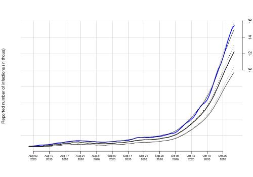
Figure 10: The effect of cluster tracing on the reported number of daily infected persons. Observed cluster with size $20$ or greater are traced with effectiveness of $C_{eff}=0.35$. The base case is given in solid blue. Different reporting rates ($p_{0}=0.2,0.5)$ are given in black solid and dotted lines respectively. The simulation is based on 10,000 trials and the mean case is given by thick lines whereas the upper and lower $5\%$ cases are given by thin lines.

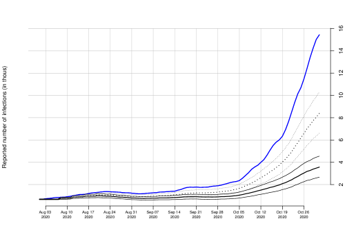
Figure 11: The effect of cluster tracing on the reported number of daily infected persons. Observed cluster with size $5$ or greater are traced with effectiveness of $C_{eff}=0.35$. The base case is given in solid blue. Different reporting rates ($p_{0}=0.2,0.5)$ are given in black solid and dotted lines respectively. The simulation is based on 10,000 trials and the mean case is given by thick lines whereas the upper and lower $5\%$ cases are given by thin lines.

6 Appendix

Lemma 1.

Let $X\sim\mathcal{NB}(p,r)$ with parameters $p\in(0,1)$ and $r>0$. If $Z_{1},Z_{2},\ldots$ are i.i.d. $Bernoulli(p_{0})$ variables, then

$$Y:=\sum_{j=1}^{X}Z_{j}\sim\mathcal{NB}(q,r)\ \ \mbox{with}\ \ q=\frac{p}{p+p_{0}-p_{0}\cdot p}.$$

Proof:   Notice first that for $X=n$ given, the distribution of $Y|X=n$ is $Binomial(n,p_{0})$. Furthermore, if $X\sim\mathcal{NB}(p,r)$ then $X\sim Poisson(\lambda)$ with $\lambda\sim Gamma\big{(}r,p/(1-p)\big{)}$; see (1). From these we get for $k\in\mathds{N}\cup\{0\}$,

$$P(Y=k) =\sum_{n=k}^{\infty}P(Y=k|X=n)\cdot P(X=n)$$

$$=\sum_{n=k}^{\infty}\left(\begin{array}[]{c}n\\ k\end{array}\right)p_{o}^{k}(1-p_{0})^{n-k}\int_{0}^{\infty}\frac{e^{-\lambda}\lambda^{n}}{n!}\cdot f_{r,\frac{p}{1-p}}(\lambda)d\lambda$$

$$=\int_{0}^{\infty}\frac{(p_{0}\cdot\lambda)^{k}e^{-\lambda}}{k!}\sum_{s=0}^{\infty}\frac{(1-p_{0})^{s}\lambda^{s}}{s!}\cdot f_{r,\frac{p}{1-p}}(\lambda)d\lambda$$

$$=\int_{0}^{\infty}\frac{(p_{0}\cdot\lambda)^{k}e^{-p_{o}\cdot\lambda}}{k!}\cdot f_{r,\frac{p}{1-p}}(\lambda)d\lambda$$

$$=\int_{0}^{\infty}\frac{\widetilde{\lambda}^{k}e^{-\widetilde{\lambda}}}{k!}\cdot\frac{1}{p_{0}}f_{r,\frac{p}{1-p}}\Big{(}\frac{\widetilde{\lambda}}{p_{0}}\Big{)}d\widetilde{\lambda},$$

where the last equality follows using the substitution $\widetilde{\lambda}=p_{o}\cdot\lambda$. Since

$$\frac{1}{p_{0}}f_{r,\frac{p}{1-p}}\Big{(}\frac{\widetilde{\lambda}}{p_{0}}\Big{)} =\frac{1}{\Gamma(r)}\Big{(}\frac{p}{(1-p)p_{0}}\Big{)}^{r}\widetilde{\lambda}^{r-1}e^{-\widetilde{\lambda}\frac{p}{(1-p)p_{0}}}$$

$$=f_{r,\frac{q}{1-q}}\big{(}\widetilde{\lambda}\big{)},$$

where $q=p/(p+p_{0}-p_{0}\cdot p)$, we get

$$P(Y=k)=\int_{0}^{\infty}\frac{\widetilde{\lambda}^{k}e^{-\widetilde{\lambda}}}{k!}\cdot f_{r,\frac{q}{1-q}}(\widetilde{\lambda})d\widetilde{\lambda},$$

which is the probability function of the $\mathcal{NB}(q,r)$ distribution.

$\Box$

References

- [1] \harvarditemAlimohamadi et al.2020Alimohamadi2020 Alimohamadi, Y., Taghdir, M., and Sepandi, M. (2020). The estimate of the basic reproduction number for novel coronavirus disease (COVID-19): a systematic review and meta-analysis. Journal of Preventive Medicine and Public Health.
- [2] \harvarditemAlthouse el al.2020Althouse2020 Althouse, B. M., Wenger, E. A., Miller, J. C., Scarpino, S. V., Allard, A., Hébert-Dufresne, L., and Hu, H. (2020). Stochasticity and heterogeneity in the transmission dynamics of SARS-CoV-2. arXiv preprint arXiv:2005.13689.
- [3] \harvarditeman der Heiden and Hamouda2020HeidenHamouda2020 an der Heiden, M. and Hamouda, O. (2020). Schätzung der aktuellen Entwicklung der SARS-CoV-2-Epidemie in Deutschland - Nowcasting. Epidemiologisches Bulletin 17, 10–16.
- [4] \harvarditemAzmon et al.2014Azmonetal2014 Azmon, A., Faes, C. and Hens, N. (2014). On the Estimation of the Reproduction Number Based on Misreported Epidemic Data. Statistics in Medicine 33, 1176–1192.
- [5] \harvarditemBest et al.2009Bestetal2009 Best, D.J., Rayner, C.W. and Thas, O. (2009). Anscombe’s Test of Fit for the Negative Binomial Distribution. Journal of Statistical Theory and Practice 3, 555–565.
- [6] \harvarditemBuitrago-Garcia al.2020Buitrago2020 Buitrago-Garcia, D. C., Egli-Gany, D., Counotte, M. J., Hossmann, S., Imeri, H., Salanti, G. and Low, N. (2020). Asymptomatic SARS-Cov-2 Infections: A Living Systematic Review and Meta-analysis. medRxiv.
- [7] \harvarditemChowell and Brauer2009ChowellBrauer2009 Chowell, G. and Brauer, F. (2009). The Basic Reproduction Number of Infectious Diseases: Computation and Estimation Using Compartmental Epidemic Models. In: G. Chowell, J.M. Hyman, L.M.A. Bettencourt and C Castillo-Chavez (eds.) Mathematical and Statistical Estimation Approaches in Epidemiology, Springer, Dordrecht, 1–30.
- [8] \harvarditemContreras et al.2020Contrerasetal2020 Contreras, S., Dehning, J., Loidolt, M., Zierenberg, J., Spitzner, F.P., Urrea-Quintero, J.H., Mohr, S.B., Wilczek, M., Wibral, M. and Priesemann, V. (2020). The Challenges of Containing SARS-CoV-2 via Test-Trace-and-Isolate. arXiv:2009.05732v2 [q-bio.PE].
- [9] \harvarditemCori et al.2013Corietal2013 Cori, A., Ferguson, N.M., Fraser, C. and Cauchemez, S. (2013). A New Framework and Software to Estimate Time-Varying Reproduction Numbers During Epidemics. American Journal of Epidemiology 178, 1505–1512.
- [10] \harvarditemDehning et al.2020aDehningetal2020a Dehning, J., Zierenberg, J., Spitzner, F.P., Wibral, M., Neto, J.P., Wilczek, M. and Priesemann, V. (2020a). Inferring Change Points in the Spread of COVID-19 Reveals the Effectiveness of Interventions. Science 369, 1–9.
- [11] \harvarditemDehning et al.2020bDehningetal2020b Dehning, J., Spitzner, F.P., Linden, M.C., Mohr, S.B., Neto, J.P., Zierenberg, J., Wibral, M., Wilczek, M. and Priesemann, V. (2020b). Model-Based and Model-Free Characterization of Epidemic Outbreaks. MedRxiv Preprint doi: https://doi.org/10.1101/2020.09.16.20187484
- [12] \harvarditemEndo et al.2020Endo2020 Endo, A., Abbott, S., Kucharski, A. J., and Funk, S. (2020). Estimating the overdispersion in COVID-19 transmission using outbreak sizes outside China. Wellcome Open Research, 5(67), 67.
- [13] \harvarditemFraser2007Fraser2007 Fraser, C. (2007). Estimating Individual and Household Reproduction Numbers in an Emerging Epidemic. PLOS ONE 2(8) 1–12.
- [14] \harvarditemHotz et al.2020Hotztal2020 Hotz, T., Glock, M., Heyder, S., Semper, S., Böhle, A., and Krämer, A. (2020). Monitoring the Spread of COVID-19 by Estimating Reproduction Numbers over Time. TU Ilmenau, Prperint. arXiv:2004.08557, 18/04/2020.
- [15] \harvarditemLinden et al.2020Lindenetal2020 Linden, M., Dehning, J., Mohr, S.B., Mohring, J., Meyer-Hermann, M. Pigeot, I., Schöbel, A. and Priesemann, V. (2020). The Foreshadow of a Second Wave: An Analysis of Current COVID-19 Fatalities in Germany. Deutsches Ärzteblatt Int. 117, 790–791.
- [16] \harvarditemLloyd-Smith et al.2005aLloydSmithetal2005 Lloyd-Smith, J.O., Schreiber, S.J., Kopp, P.E. and Getz, W.M. (2005). Superspreading and the Effect of Individual Variation on Disease Emergence. Nature 438, 355–359.
- [17] \harvarditemLloyd-Smith et al.2005bLloydSmithetalSuppl2005 Lloyd-Smith, J.O., Schreiber, S.J., Kopp, P.E. and Getz, W.M. (2005). Superspreading and the Effect of Individual Variation on Disease Emergence: Supplementary Information.
- [18] \harvarditemRobert Koch Institut2020RKI2020 Verlautbarung des Robert-Koch-Instituts (2020). Erl”auterung der Sch”atzung der zeitlich variierenden Reproduktionszahl R. Robert-Koch-Institut.
- [19] \harvarditemMeintanis2005Meintanis2005 Meintanis, S.G. (2005). Transform Methods for Testing the Negative Binomial Hypothesis. Statistica LXV, 293–300.
- [20] \harvarditemOran and Topol2020OranTopol2020 Oran, D. P. and Topol, E. J. (2020). Prevalence of Asymptomatic SARS-Cov-2 Infection. Annals of Internal Medicine.
- [21] \harvarditemRahmandad et al.2020Rahmandadetal2020 Rahmandad, H., Lim, T.Y. and Sterman, J. (2020). Estimating COVID-19 Under-Reporting Across 86 Nations: Implications for Projections and Control. MedRxiv Preprint doi: https://doi.org/10.1101/2020.06.24.20139451
- [22] \harvarditemSantos-Hövener et al.2020Santosetal2020 Santos-Hövener, C., Neuhauser, H.K, Schaffrath Rosario, A., Busch, M., Schlaud, M., Hoffmann, R., Gößwald, A., Koschollek, C., Hoebel. J., Allen. J., Haack-Erdmann, A., Brockmann. S., Ziese, T., Nitsche, A., Michel, J., Haller, S., Wilking, H., Hamouda, O., Corman, V.M., Drosten, C., Schaade, L., Wieler, L., CoMoLo Study Group, Lampert, T. (2020). Serology- and PCR-Based Cumulative Incidence of SARS-CoV-2 Infection in Adults in a Successfully Contained Early Hotspot (CoMoLo study), Germany, May to June 2020. Euro Surveill. 25(47):pii=2001752. https://doi.org/10.2807/1560-7917.ES.2020.25.47.2001752
- [23] \harvarditemStreeck et al.2020Streecketal2020 Streeck, H., Schulte, B., Kümmerer, B.M. et al (2020). Infection Fatality Rate of SARS-CoV-2 in a Super-Spreading Event in Germany. Nature Communications 11, article number: 5829 (2020). https://doi.org/10.1038/s41467-020-19509-y
- [24]