Soliton Solutions to the Curve Shortening Flow on the 2-dimensional hyperbolic plane
Fábio Nunes da Silva111Universidade de Brasília, Department of Mathematics, 70910-900, Brasília-DF, Brazil, fabionuness@ufob.edu.br Keti Tenenblat222 Universidade de Brasília,
Department of Mathematics,
70910-900, Brasília-DF, Brazil, K.Tenenblat@mat.unb.br Partially supported by CNPq Proc. 312462/2014-0, Ministry of Science and Technology, Brazil and FAPDF/Brazil grant 0193.001346/2016.
Abstract
We show that a curve is a soliton solution to the curve shortening flow if and only if its geodesic curvature can be written as the inner product between its tangent vector field and a fixed vector of the 3-dimensional Minkowski space. We use this characterization to provide a qualitative study of the solitons. We show that for each fixed vector there is a 2-parameter family of soliton solution to the curve shortening flow on the 2-dimensional hyperbolic space. Moreover, we prove that each soliton is defined on the entire real line, it is embedded and its geodesic curvature converges to a constant at each end.
A family of curves , ,
on a 2-dimensional Riemannian manifold is said to be a solution
to the Curve Shortening Flow (CSF) with initial condition
, if it satisfies the following equation
(1.1)
where
is the geodesic curvature and
is the unit vector field normal to
for each .
Epstein and Gage [6] showed that when , the CSF is
geometrically the same if tangential components are added to the right hand side of
the differential equation (1.1). Therefore, one can define that a 1-parameter
family of curves
,
is a solution to the CSF in with initial condition , if it satisfies
(1.2)
where is the cannonical inner product on ,
is the curvature and is the unit vector field normal to
for each . The name curve shortening flow is justified by the fact that when the curves of the family
are closed, then the length of the curves decreases along the flow, i.e.,
it is a gradient type of flow for the arc length functional.
Grayson [12] observed that the CSF is also known as the curvature flow or
the heat flow for isometric immersions.
According to Epstein and Gage [6],
the original motivation for studying equation (1.1) was to find a new and maybe more natural proof of the existence of closed geodesics on Riemannian manifolds.
However, the first results in this direction were obtained by
Grayson [13] em 1989. But equation (1.1)
for the Euclidean plane was investigated earlier by several authors
[2], [7], [8], [9], [10] e [12].
An important class of solutions to the CSF are those that evolve by isometries or homotheties. Such solutions are called self-similar solutions and solitons
if they evolve just by isometries. On the Euclidean plane, the straight lines are not affected by the flow and they are considered to be trivial solutions.
Circles evolve homothetically to a point in finite time. The Grim Reaper curve given by the graph of the function evolves by a flow of translations. Giga [11] proved that this is the unique curve on the plane that evolves by translations. An example of a plane curve that evolves by isometries of the plane is
the yin-yang spiral. Abresch-Langer [2] and Epstein-Weinstein [7] investigated the closed curves, not necessarily simple, that evolve by homotheties. Halldorsson [14] concluded the description of
all self-similar solutions on the plane.
Some authors studied classes of solutions to the CSF on the plane and proved that
after a certain time the flow evolves into a self-similar one. First, Gage [8] [9] showed that closed convex curves
on evolve into circular curves after a certain time. Then
Gage and Hamilton [10] showed that convex closed curves collapse into a point.
Grayson [12] proved that closed embedded curves evolve to circular curves and then they collapse into a point at a finite time.
Moreover, Angenent [3], under more general conditions, proved that the CSF
evolves in a sense into a self-similar flow, showing the importance of self-similar solutions.
One should point out that, when the ambient space is not the Euclidean plane, there are very few results on self-similar solutions to the CSF.
In 2015, Halldorsson [15] classified all the self-similar solutions on the Minkowski plane. Dos Reis and Tenenblat [5] caracterized and described all the soliton solutions on the sphere . Some results on the CSF for Riemannian manifolds different from the plane can be found in [10], [13], [16] and [20], among others. Moreover, Angenent, [4] studied the topology of the closed geodesics on compact surfaces by using the CSF.
In this paper, we will study the soliton solutions of curve shortening flow on the 2-dimensional hyperbolic space , where is the 3-dimensional Minkowski space.
2 Main Results
We consider the 3-dimensional Minkowki space as , where is the 3-dimensional vector space and is the Minkowski metric defined by
Let be a regular curve parametrized by arc length . We denote by the tangent vector field, the unit normal vector field and the geodesic curvature of . A one parameter family of curves is called a curve shortening flow (CSF) with initial condition , if
(2.1)
where is the geodesic curvature and is the unit normal vector field of . When is a geodesic i.e. , then the family gives a trivial solution to the CSF. Our goal is to study the case when evolves by a 1-parameter family of isometries of .
Definition 2.1.
Let be a solution to the curve shortening flow (2.1) on , with initial condition . We say that is a soliton solution to the curve shortening flow if there is a 1-parameter family of isometries such that and
for all , where is the identity map.
We remark that an isometry of is an element of the Lie group that preserves , where is the transpose of and
Theorem 2.2.
Let be a regular curve parametrized by arc length. Then , , is a soliton solution to the curve shortening flow if, and only if, there is a vector such that
(2.2)
where is the unit tangent vector field and is the geodesic curvature of .
We observe that when is a geodesic of ,
then it is a planar curve and hence there exists a vector such that
The following theorem describes the qualitative behaviour of the soliton solutions to the CSF in
Theorem 2.3.
For any , there is a 2-parameter family of non-trivial soliton solutions to the curve shortening flow on the 2-dimensional hyperbolic space. Each soliton solution is an embedded curve on , defined for all . Moreover, at each end, the curvature function tends to one of the following constants .
3 Proofs of the main results
In this section we prove our main results.
Proof of Theorem 2.2. Suppose that is parametrized by arc length . If is a soliton solution to the CSF, then is solution to (2.1), where is a family of isometries of .Taking the derivative of at , we have
It follows from definition of the CSF that
In particular, for , we have
is an element of the Lie algebra of the Lie group . Let be a basis of , where
Then , for real numbers .
By simple computations, we can prove that , where and . Therefore,
Conversely, let be a curve in parametrized by arc length , such that for a vector . Without loss of generality, up to isometries of , we can consider to be a multiple of if is a timelike vector, a multiple of if is a lightlike vector and a multiple of if is a spacelike vector. Thus, depending on the type of the vector , we can write the curvature as where , and .
Now, we define the evolution of in to be , where
(3.8)
(3.12)
and for each
A straightforward computation shows that
Thus,
where the last equality follows from the fact that isometries preserve geodesic curvature.
Therefore, is a soliton solution to the CSF.
It follows from Theorem 2.2 that the study of the solitons solutions to the CSF on the 2-dimensional hyperbolic space is reduced to describing the curves that satisfy Equation (2.2) for some vector . Up to isometries of we consider as being , where , if is a timelike vector, if is a lightlike vector and if is a spacelike vector. Our next result characterizes (2.2) in terms of a system of differential equations.
Proposition 3.1.
Let be a regular curve parametrized by arc length . Consider the vectors
(3.13)
For each , define the functions
where and are the unit vector fields tangent and normal to , respectively. For a fixed ,
is satisfied, for all if, and only if, the functions , and satisfy the system
(3.14)
with initial condition satisfying
(3.15)
For such functions, the expression is equal to the right hand side of (3.15), for all . Moreover, is a decreasing function.
Proof.
The vector fields , and satisfy the following system of equations
(3.16)
Taking the inner product with , we get that , and satisfy the system of equations
(3.17)
Suppose that for all . Then substituting into (3.17), we obtain (3.14). Note that,
Therefore, is constant for all . In particular, for , we obtain (3.17). Moreover, it follows from the third equation of the system (3.14) that the function is decreasing.
Conversely, suppose that the functions , and satisfy (3.14) and (3.15) for each . Since (3.17) holds, we have
i.e.,
for all . For eaxch , in order to conclude that , for all , we will assume that at some point . Then this will occur on some interval around . Hence for . Therefore, will be orthogonal to and for all . Thus, will be parallel to for all . But is a constant vector for each , so this can only happen at some isolated points of a curve in , which is a contradiction. Therefore, for all and for each .
∎
Our next proposition shows how a solution of the system (3.14), with initial conditions satisfying (3.15), is related to a soliton solution to the CSF.
Proposition 3.2.
Given a solution to the system (3.14) on some interval with fixed and initial conditions satisfying (resp. and ), there exists a smooth curve parametrized by arc length , such that its tangent and normal unit vector fields and satisfy
(3.20)
where (resp. and ).
Proof.
Define . Thus, up to isometries of , there exists an unique curve , whose curvature is i.e. and its tangent and normal unit vector fields and satisfy the system (3.16). The curve is uniquely determined by the initial conditions , and , that can be chosen such that
where (resp. and ). A straightforward computations shows that (3.15) and (3.16) imply
Let be a regular curve parametrized by arc length given by . The function defined by (3.20) has the following geometric interpretation.
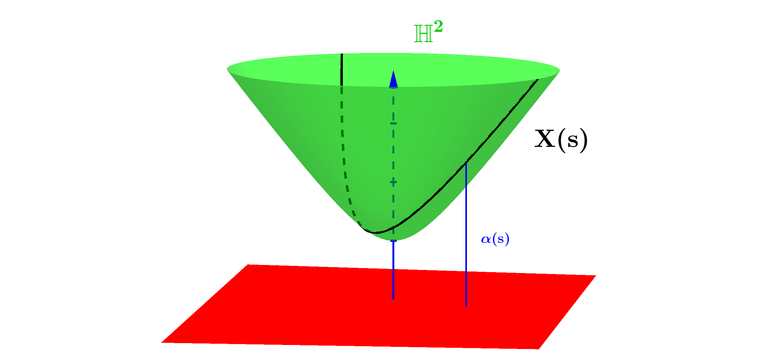
•
If (timelike vector), then for all . Moreover, is the height function with respect to the vector
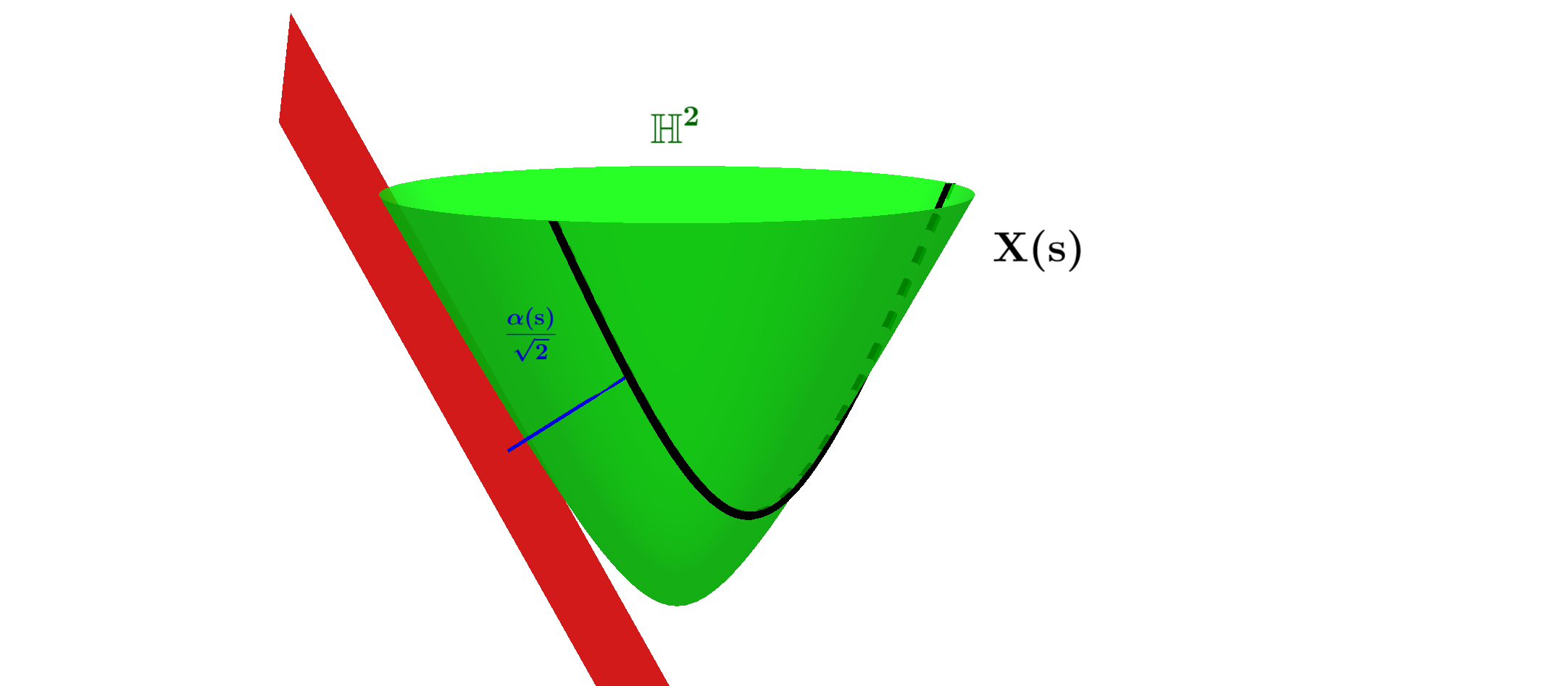
•
If (lightlike vector), then for all . Moreover, is the height function with respect to the vector
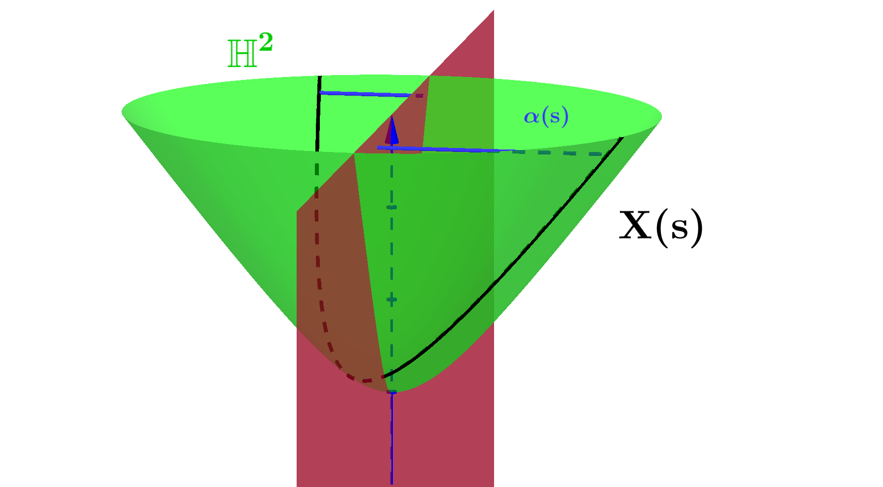
•
If (spacelike vector), then for all . Moreover, is the height function (with sign) with respect to the vector
Figure 1a (resp. 1b and 1c) provides a geometric illustration of the function as a height function with respect to vector (resp. and .)
(a)
(b)
(c)
Figure 1: Geometric interpretation of the functions .
As we have seen in Propositions 3.1, 3.2 and Remark 3.3, the investigation of the soliton solutions to the CSF on the 2-dimensional hyperbolic space is equivalent to studying the solutions of the system
(3.21)
for each constant and initial condition where
(3.22)
These are disjoint sets and if the initial condition
(resp. or ) then the solution defined on the maximal interval will be contained in (resp. or ) for all .
From now on, using (3.21), we will prove a series of lemmas that will provide the proof of the main result (Theorem 2.3). Namely, we will prove that for any initial condition, the solutions of (3.21) and hence the associated soliton solutions to the hyperbolic space are defined on the whole . Moreover, we will analize the behaviour of the curvature function of the solitons at each end.
In the first lemma we will study the solution of (3.21) such that the function is constant. As we will see such solutions (that will be called trivial) only exit on .
Lemma 3.4.
Let be a non null solution of (3.21) defined on the maximal interval , and initial condition , where , and are given by (3.22). Then
the function , , where is a real constant if, and only if, , and for all Moreover,
If , it follows from (3.21) that for all . Using the equation , where , we obtain for all . Hence, , are singular solutions of (3.21) in .
If is not a singular solution, then and it follows from (3.21) that
for all . Using the relation , where , we conclude that
and hence the function is also constant. Since is not a singular solution, it follows that and .
Therefore, , , and , for all . This concludes the proof.
∎
It follows from Lemma 3.4 that when is a constant function then the functions and are linear in and its corresponding soliton solutions to the CSF are curves of constant curvature i.e. geodesics when or planar curves with curvature .
In this context, we define a trivial solution of (3.21), when is a constant function. From now on, we will study only non trivial solutions of (3.21). It follows from Lemma 3.4 that there are no trivial solutions of (3.21) in .
On our next lemmas we will study the solutions of (3.21) contained in and those contained in separately.
Lemma 3.5.
Let be a solution of (3.21) defined on the maximal interval , and initial condition , where and are given by (3.22).
i)
If has a critical point then it is a global minimum point of . Moreover, there exists always such that is strictly monotone on the intervals and .
ii)
If is a critical point of , then and is a local minimum (resp. maximum) point of if, and only if, (resp. ).
Proof.
i) Let be a critical point of . Note that for all whenever . Taking the second derivative of and using (3.21) at , we have
Hence, is a global minimum point of . Therefore, has at most one critical point. If there are no critical points then is trictly monotone on .
ii) Let be a critical point of . Then and because for all . Since , it follows that for all , where . Thus,
Hence, . Taking the second derivative of and using (3.21) at , we have
(3.23)
This concludes the proof of ii).
∎
Lemma 3.6.
Let be a solution of (3.21) defined on the maximal interval , and initial condition , where is given by (3.22).
i)
If in , then is strictly increasing in , is bounded and it has at most one critical point in . Moreover, , and
ii)
If in , then is strictly decreasing in , is bounded and it has at most one critical point in . Moreover, , and
Proof.
i) If , then it follows from Lemma 3.5 that has only local maximum points i.e. has at most one critical point. The positive function is bounded and there exists such that is strictly increasing on . Thus, it follows from equation that we can take such that and are bounded and monotone on . The interval is maximal, hence Since the limits , and exist, we obtain
that and . Using the fact that the function is decreasing, we get that for all
We claim that is ununbounded on . In fact, assume by contradiction that the strictly increasing function is bounded on . Thus, it follows from equation that we can take such that and are bounded and monotone on . Hence, there exists such that and is a singular (trivial) solution in , which contradicts Lemma 3.4. Therefore,
Now, assume by contradiction that the strictly decreasing and negative function is bounded on . Since , it follows that the function is unbounded and positive on , because we showed that is unbounded on . Thus, we can choose such that for all . Using the equations of (3.21), we obtain
(3.24)
Hence
for each . But this contradicts the fact that is unbounded. Therefore, is unbounded and .
Finally, if is unbounded on , , then we can choose again such that for all . Using (3.24), we obtain
this is a contradiction, because i.e. and .
ii) This proof is analogous to the proof of item i).
∎
Lemma 3.7.
Let be a solution of (3.21) defined on the maximal interval , and initial condition , where is given by (3.22). Then there exists a unique such that .
Proof.
Assume by contradiction that such an does not exist. Then, either or for all . If , then is strictly decreasing. Taking we have for all . Since , then for all . Hence, the functions are bounded and monotone in , and exists, because . Thus, there exists a point such that . Therefore, and is a singular (trivial) solution of (3.21), which contradicts Lemma 3.4. In a similar way, we can prove that for all cannot occur.
Therefore, there is an such that . It follows from Lemma 3.5, that is a global minimum of the function . Hence, is unique.
∎
In the next three lemmas, we will suppose that and that has only one critical point. Note that, this hypothesis only excludes the case presented in Lemma 3.6 because it follows from Lemma 3.4 that has at most one critical point when and Lemma 3.7 shows that has a unique critical point, when .
Lemma 3.8.
Let be a solution of (3.21) defined on the maximal interval , and initial condition , where and are given by (3.22).
If has one critical point, then .
Proof.
Let be the global minimum point of . Thus, is monotone on the intervals and . Assume by contradiction that is bounded on the intervals and . Since the functions , and satisfy , where , then the functions and are bounded and monotone on and . The limits and exist, because . Thus, there are points and such that and . Hence, , and is a set of singular (trivial) solutions of (3.21), which contradicts Lemma 3.4.
Therefore, we conclude that the function is unbounded on the intervals and , and moreover .
∎
Lemma 3.9.
Let be a solution of (3.21) defined on the maximal interval , and initial condition , where and are given by (3.22).
If has one critical point, then and .
Proof.
Let be the global minimum point of . Then for all and for all . Moreover, is unbounded and monotone on the intervals and .
Assume by contradiction that the function is bounded on . Since , where , then it follows from Lemma 3.7 that the function is unbounded and negative on i.e. there exists such that and for all . Thus, using (3.21) for each , we obtain
that is,
for each which contradicts Lemma 3.8. Therefore, is unbounded on .
In a similar way, we can prove that the function is unbounded on .
Since is decreasing on , it follows that and . ∎
Lemma 3.10.
Let be a solution of (3.21), with , defined on the maximal interval and initial condition , where and are given by (3.22).
If has one critical point, then the function is unbounded on and it has only two critical points.
Proof.
Let be the global minimum point of . The arguments consist in studying the existence and the properties of the critical points of .
Claim. If does not have any critical point on , then on and on . In fact, suppose that for all . At , and . Moreover, i.e. is an increasing function on , and . It follows from Lemma 3.9 that and . We also know that is negative on and positive on . Thus, there are and such that for all . Hence, for all and
i.e.,
Therefore,
for all .
Taking the limit when and , using the fact that is increasing and Lemma 3.9, we obtain that
i.e.,
Thus, using that is increasing, we conclude that on and on . This proves our Claim.
Still assuming that does not have any critical point, we define the positive functions and (observe that ). Taking the derivatives of and and using (3.21), we obtain and . It follows from our Claim that the functions and are decreasing when and they are increasing when and
for all , where . Hence, the functions and are positive, monotone and bounded on the interval . Similarly one shows that the functions and are positive, monotone and bounded on . Thus, we conclude that there exist such that
Hence,
These inequalities contradict Lemma 3.8. Hence, the function has at least one critical point on each interval and . From item ii) of Lemma 3.5 we have that has only one local minimum and it has only one local maximum i.e. for all and is bounded on the interval . This concludes the proof. ∎
Lemma 3.11.
Let be a solution of (3.21) defined on the maximal interval , and initial condition , where and are given by (3.22). Then .
Proof.
From Lemmas 3.6 and 3.10 we have that is bounded. Let be such that , for all . Using (3.21), we obtain,
(3.25)
for each . If has a global minimum point, then it follows from Lemma 3.8 that . Hence, .
If does not have any critical point and (resp. ) for all , then it follows from Lemma 3.6 that and (resp. and ). Using (3.25), we conclude that (resp. ). Therefore, .
∎
We will now study the solutions of the system (3.21), with initial conditions on .
We will first classify the singular points of the system that are in the set .
Lemma 3.12.
Let be the differential vector field given by
where . Then and are the singular points of and the eigenvalues of and are given respectively by
(3.26)
Proof.
Note that, if , then and . Hence, and are the singular points of . The tangent plane in each singular point is defined by . Thus,
Hence is an eigenvalue of if there is a non null
vector such that
i.e.
In Lema 3.12, we saw that are saddle points
for the vector field on , i.e., ,
are singular solutions of (3.21). If the functions and are identically
zero then the corresponding curve is the intersection of the upper half hyperboloid
with the plane going through the origin, orthogonal to . Hence both singular solutions of the system correspond to the same curve.
In order to study the non trivial solutions of the system
(3.21), we consider the singular point and a solution of the system with initial condition . Since the eigenvalues of the linearized system at the singular point are not zero, it follows that the local behavior of the system
(3.21) is equivalent to the linearized one. Hence, there exist initial conditions
such that and .
We define the unstable and stable sets as
(3.27)
From Lemma 3.4 we know that, if the function is a non zero constant,i.e., , for all , then . Our next result provides two non trivial solutions of the system (3.21), , defined on , with initial conditions on the set . They are particular cases of the solutions
obtained in Lemma 3.4 with the constant of integration being zero. Moreover, we also obtain the soliton solutions corresponding to these soltions.
Proposition 3.13.
Let be a solution of (3.21) defined on the maximal interval , and , where is given in (3.22). Then, (resp. ), satisfy (3.21) with initial condition (resp. ). Moreover,
i)
The curve
(3.28)
where is the soliton solution to the CSF in which corresponds to the solution of (3.21);
ii)
The curve
where is the soliton solution to the CSF in which corresponds to the solution of (3.21)
Proof.
Straightforward computations show that and satisfy (3.21) with initial conditions and respectively.
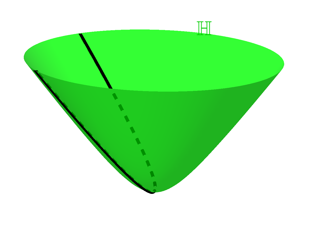
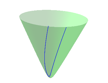
In Figure 2, we illustrate the curve in
given by (3.28) with .
Figure 2: Soliton solution to the CSF with , fixed vector and constant curvature ().
In the following lemmas, we study the behavior of the functions , and when is a non trivial solution of the system
(3.21) and initial condition .
Lemma 3.14.
Let be a non trivial solution of (3.21) defined on the maximal interval , and initial condition , where is given in (3.22). If is a critical point of , then is the global minimum (resp. maximum) of if, and only if, (resp. ). Moreover, there exists always such that the function is monotone on the intervals and
Proof.
Let be a critical point of , then . It follows from (3.21) that
(3.29)
Note that, if and , then is constant, because is a singular (trivial) solution of (3.21).
Therefore, it follows from (3.29) that is a local minimum point of if . If there is another critical point of such that and are consecutive, then , because is a local minimum point. Thus, and is a local minimum point , this is a contradiction. Therefore, if , then is a global minimum of .
If , it follows from (3.29) that a local maximum point of . The proof that is a global maximum point of is analogue to the previous case.
Since the function has at most one critical point, there exists always such that the function is monotone on the intervals and
∎
We observe that if for a solution
of (3.21) with , the function does not have a crtitical point, then is monotone on .
Moreover, it follows from Lemma 3.14, that for any solution of (3.21) with , the functions and
do not have critical points.
Lemma 3.15.
Let be a non trivial solution of (3.21) defined on the maximal interval , and initial condition , where is given by (3.22). Consider and given by (3.27). If (resp. ), then (resp. ).
Proof.
It follows from Lemma 3.14 that there exits such that is monotone on the intervals and . If assume by contradiction that is bounded on . Since , it follows that the functions and are bounded and monotone on and the limit exists.
Hence, there exists such that , and is a singular solution of (3.21). But the system (3.21) does not have any singular solution on the set . Therefore, .
Similarly, when one proves that .
∎
Lemma 3.16.
Let be a non trivial solution of (3.21) defined on the maximal interval , and initial condition , where is given in (3.22).
i)
If is a critical point of . Then and . If , then is a local minimum (resp. maximum) point of if, and only if, (resp. ). If , then is a local minimum (resp. maximum) point of if, and only if, (resp. ).
ii)
The function has at the most a finite number of critical points.
Proof.
i)
Let be a critical point of . If , it follows from that . Thus, i.e. . Hence, it follows from Lemma 3.4 that the solution of (3.21) with initial condition is a trivial solution, which contradicts the hypothesis. Therefore, . If , then and from we have that , which also contradicts the hypothesis. Hence, and . Moreover, taking the second derivative of at , we obtain (3.23). This concludes the proof of the item i).
ii) Note that, it follows from Lemma 3.14 that there exists always such that does not change sign on each interval and . We will prove for the interval , since similar arguments can be used for the interval . If i.e. , then it follows from item i) that has at most a finite number of critical points on . If , then it follows from Lemma 3.15 that .
Assume that for all , then there exists such that for all . If the function , which is monotone, is always positive, then for all , i.e. has no critical
on . Now, consider such that for all . Assume by contradiction that there are , two local maximum points of . From item i), we obtain that there are such that , , , . It follows from
that and . Thus, from we obtain i.e. and from we conclude i.e. , this is a contradiction. Therefore, has at most one local maximum point on the interval .
Analogously, assume that for all , then there exists such that for all . If the monotone function is always positive, then for all , and hence has no critical point on . Now, we consider such that for all . Assume by contradiction that there are , two local maximum points of . From item i) we obtain that there are such that , , , . It follows from that and . Thus, from we obtain that i.e and from we conclude that i.e. , this is a contradiction. Therefore, has at most one local maximum point on the interval .
Similar arguments for the interval imply that has at most a finite number of critical points on .
∎
The following lemma shows that the function is bounded and hence the curvature of the soliton on is bounded.
Lemma 3.17.
Let be a non trivial solution of (3.21) defined on the maximal interval , with initial condition , where is given by (3.22). Then the function is bounded on .
Proof.
It follows from Lemma 3.14 that there exists such that is monotone on the intervals and . Moreover, from Proposition 3.2 we have that is monotone.´
If , where is a singular point, then and is bounded on for any fixed. Similarly, if , then and is bounded on , fixed.
We will now consider the cases when the initial condition belongs to or .
If assume by contradiction that is unbounded on , then it follows from Lemma 3.16 that there exists such that and for all . Thus, , because and for all . From Lemma 3.14 we have that does not sign on .
If on , then is strictly decreasing on this interval. Thus, it follows from Lemma 3.15, that . Hence, can be chosen so that is decreasing and positive for all . Therefore, using (3.21) and the fact that , we obtain
i.e.,
which contradicts Lemma 3.15, because . Hence, is bounded on .
If on , then is strictly increasing on this interval. Thus, it follows from Lemma 3.15 that . Hence, can be chosen so that is increasing and negative for all . Therefore, using (3.21) and the fact that , we obtain
i.e. ,
which contradicts Lemma 3.15, because . Hence, is bounded on .
When , the similar arguments show that is bounded on .
Therefore, the function is bounded on .
∎
Our next lemma provides the behavior of the function .
Lemma 3.18.
Let be a non trivial solution of (3.21) defined on the maximal interval , and initial condition , where is given by (3.22). Consider and given by (3.27). If (resp. ), then (resp. ).
Proof.
The proof follows from Lemmas 3.15 and 3.17 and the fact that .
∎
Lemma 3.19.
Let be a non trivial solution of (3.21) defined on the maximal interval , and initial condition , where is given by (3.22). Then .
Proof.
It follows from Lemma 3.17 that is bounded on the interval . Let be such that for all . Using (3.21), we obtain that
(3.30)
for all . We will now show that and .
If , then from Lemma 3.15 we have that is unbounded on for any fixed. Hence, it follows from (3.30) that . It follows from the definition of that when . Since , we conclude that .
If , then from Lemma 3.15 we have that is unbounded on for any fixed. Hence, it follows from (3.30) that . It follows from the definition of that when . Since , then .
Therefore, .
∎
Lemma 3.20.
Let be a non trivial solution of (3.21), with and initial condition , where , and are given by (3.22). Then and the corresponding soliton solution to the CSF on are defined for all . Moreover, at each end the curvature of converges to one of the following constants .
Proof.
Since is a soliton solution to the CSF corresponding to , then . Thus, Lemmas 3.6, 3.10, 3.14 and 3.17 imply that is bounded on and it has at most a finite number of critical points. Thus, the limits exist. In particular, when then . Similarly, when then . In these cases, the curvature function converges to zero at and
, respectively.
If , then and it follows from , where that
Using (3.21), Lemmas 3.8, 3.9, 3.15, 3.18 and L’Hospital rule, we obtain
Therefore, and .
∎
Finally, we will prove our main theorem.
Proof of Theorem 2.3. For any vector , without loss generality we can consider , where and
Let be a solution of (3.21) defined on the maximal interval , and initial condition satisfying
i.e., , where , and are the disjoint sets given by (3.22).
Moreover, it follows from Proposition 3.2 that there is a soliton solution to the CSF, with curvature , such that the relations
are satisfied, where and are the unit vector fields tangent and normal to .
Thus, the initial conditions of (3.21), which are given by two constants, determine the soliton solution in each case. Therefore, for each fixed vector there is a 2-parameter family of non trivial soliton solutions to the CSF in .
Moreover, it follows from Lemmas 3.4, 3.11 and 3.19 that each soliton solution is defined for all , i.e. and Lemma 3.20 shows that the curvature at each end converges to one of the following constants .
Note that, from Lemmas 3.4, 3.5 and 3.14 we know that there exists such that is strictly monotone on the intervals and . Since describes the Euclidean height of with respect to a fixed plane, then does not have self-intersections in each one of the intervals and . Therefore, is embedded if is monotone in .
If is not monotone in then has only one critical point. Suppose that has some self-intersection and consider the simple region bounded by with , and the external angle between the tangent vectors and , which is at the most . By Gauss-Bonnet’s theorem, we obtain
This is a contradiction. Hence, the soliton solution to the CSF in does not admit self-intersections. Note that, is already embedded on the intervals and and from Lemmas 3.8 and 3.15 we have that the two ends of the curve are unbounded. Therefore, is an embedded curve.
4 Visualizing some Soliton Solutions to the CSF on
In this setion, we visualize some examples of soliton solutions to the CSF on the hyperbolic space. In order to do so, we use the following parametrization.
for
If a curve of is parametrized by arc lentgh, then
the functions
and satisfy the following system of ODEs
(4.1)
where is the curvature of . The first equation follows from the fact that
the curve is parametrized by arc lentgh and the second one from the expression of the curvature of .
In Theorem 2.2, we saw that the curvature of a soliton solution to the CSF on is determined by its tangent vector field and a non zero fixed vector .
We use (4.1) and the software Maple to plot examples of such solitons.
In each example, we visualize the curve on the three models of the 2-dimensional hyperbolic space, namely the hyperboloid, the Poincaré disk and the upper half space.
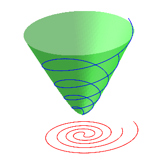
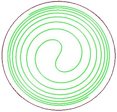
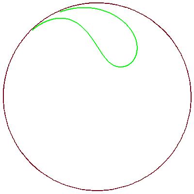
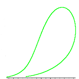
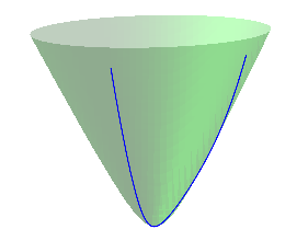
In Figure 3 a), the blue curve on the hyperboloid provides the visualization of a soliton solution to the CSF on whose curvature is given by and . The red curve is the Euclidean orthogonal projection of on the plane that contains the origin and it is orthogonal to the vector . In Figures 3 b) and c) we visualize the same soliton on the Poincaré disk and on the half space model respectively.
(a)
(b)
(c)
Figure 3: Soliton solution to the CSF on with fixed vector and .
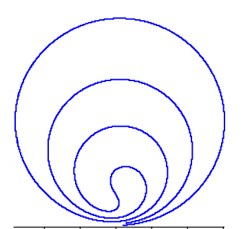
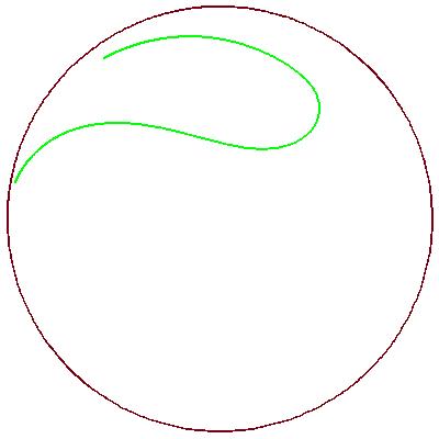
In Figure 4 a), the blue curve provides the visualization
of a soliton solution to the CSF on whose curvature is given by and . In Figures 4 b) and c) we visualize the same soliton on the Poincaré disk and on the half space model respectively.
(a)
(b)
(c)
Figure 4: Sóliton do fluxo FRC em com vetor fixado e .
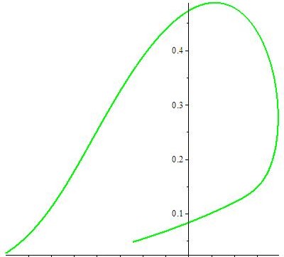
Finally, in Figure 5 a), the blue curve provides the visualization
of a soliton solution to the CSF on whose curvature is given by and . In Figures 4 b) and c) we visualize the same soliton on the Poincaré disk and on the half space model respectively.
We point out that this soliton has non constant curvature and hence it is different from
the one given in Proposition 3.13. In fact, in order to obtain
Figure 5, we used initial condition
and for the system (4.1), i.e., and .
Hence the curvature is not constant.
In Figures 5 b) and c) we visualize the soliton given in Figure 5 a)
on the Poincaré disk and on the half space model respectively.
(a)
(b)
(c)
Figure 5: Sóliton do fluxo FRC em com vetor fixado e .
Aknowlegment: The first author aknowledges the support given by the Universidade
Federal do Oeste da Bahia during his graduate program at the Universidade de Brasília, when this research was undertaken.
References
[1]
[2] Abresch, U.; Langer, J. The normalized curve shortening flow and homothetic solutions, Journal Differential Geometry 23, n. 2, p. 175–196 (1986).
[3] Angenent, S. B. On the formation of singularities in the curve shorteningow, Journal of Differential Geometry, v. 33, 601-633 (1991).
[4] Angenent, S. B. Curve shortening and the topology of closed geodesies on surfaces, Annals of Mathematics, v.162, 1187-1241 (2005).
[5] Dos Reis, H. F. S.; Tenenblat, K. Soliton solutions to the curve shortening flow on the sphere, Proc. Amer. Math. Soc., v. 147, 4955-4967 (2019).
[6] Epstein, C.L., Gage, M. The curve shortening flow. In: Chorin A.J., Majda A.J. (eds) Wave Motion: Theory, Modelling, and Computation. Mathematical Sciences Research Institute Publications, vol 7. Springer, (1987).
[7] Epstein, C.L.; Weinstein, M.I. A stable manifold theorem for the curve
shortening equation, Comm. Pure Appl. Math., v. 40, 119-139 (1987).
[8] Gage, M. E., An isoperimetric inequality with applications to curve shortening, Duke Mathematical Journal, v. 50, n.4, p. 1225–1229 (1983).
[9] Gage, M. E., Curve shortening makes convex curves circular, Inventiones mathematicae, v. 76, n.2, p. 357–364 (1984).
[10] Gage, M. E.; Hamilton, R. S., The heat equation shrinking convex plane curves, Journal Differential Geometry, v.23, p. 69-96 (1986)
[11] Giga, Y., Surface evolutions equations. A level set approach, Monographs in Mathematics, vol. 99, Birkhauser, Basel, 2006.
[12] Grayson, M. A. The heat equation shrinks embedded plane curves to round a points, Journal Differential Geometry, v.26, p. 285-314 (1987)
[13] Grayson, M. A. Shortening embedded curves, Annals of Mathematics, v. 129, n.1, p. 71–111 (1989).
[14] Halldorsson, H. P. Self-similar solutions to the curve shortening flow, Transactions of the American Mathematical Society, v. 364, n. 10, p. 5285–5309 (2012).
[15] Halldorsson, H. P. Self-similar solutions to the mean curvature flow
in the Minkowski plane , J. Reine Angew. Math., v. 704, 209–243 (2015).
[16] Ma, L.; Chen, D. Curve shortening in a Riemannian manifold, Annali di Matematica v. 186, p. 663-684 (2007)
[17] O’Neill, B. Semi-riemannian geometry with applications to relativity. Academic Press 103, (1983).
[18] Palis, J.; Melo, W. geometric theory of dynamical systems an introduction, Translated by A. K. Manning, Springer-Verlag New York (1982).
[19] Sotomayor, J. Equações diferenciais ordinárias, Editora Livraria da Física (2011).
[20] Zhou, H. Curve Shortening Flows in warped product manifolds, Transactions of the American Mathematical Society, Proc. Amer. Math. Soc., v. 145, 4505-4516 (2017).