Implicit Bias of Linear RNNs

Abstract

Contemporary wisdom based on empirical studies suggests that standard recurrent neural networks (RNNs) do not perform well on tasks requiring long-term memory. However, precise reasoning for this behavior is still unknown. This paper provides a rigorous explanation of this property in the special case of linear RNNs. Although this work is limited to linear RNNs, even these systems have traditionally been difficult to analyze due to their non-linear parameterization. Using recently-developed kernel regime analysis, our main result shows that linear RNNs learned from random initializations are functionally equivalent to a certain weighted 1D-convolutional network. Importantly, the weightings in the equivalent model cause an implicit bias to elements with smaller time lags in the convolution, and hence shorter memory. The degree of this bias depends on the variance of the transition kernel matrix at initialization and is related to the classic exploding and vanishing gradients problem. The theory is validated in both synthetic and real data experiments.

1 Introduction

Over the past decade, models based on neural networks have become commonplace in almost all machine learning applications. A key feature about this class of models is that, in principle, they do not require an explicit design of features but instead rely on an implicit learning of “meaningful” representations of the data. This makes neural network models attractive from the point of view of machine perception where raw signals are inputs to the model. While neural networks have become ubiquitous in practical applications, several theoretical aspects of them largely remain a mystery. Of significant importance is the lack of understanding of the potential implicit biases that these representations bring to the predictions of the model.

This paper aims to understand the implicit bias behaviour of Recurrent Neural Networks (RNN). Several machine learning tasks require dealing with sequential data with possibly varying lengths of input sequences. Some example tasks include automatic speech recognition, language translation, and image captioning, among others. In such tasks the simplest architecture is an RNN. Due to their simplicity, these models may be preferred over their complex descendants, Long Short-term Memory (LSTM) networks, in applications demanding interpretability.

A common critique of RNNs trained using gradient descent is their poor performance at tasks requiring long-term dependence [BSF94]. However, we lack a quantitative understanding of this phenomenon. In this paper, we provide a rigorous characterization for the implicit bias of RNNs towards short-term contexts. This characterization can suggest bias-correction strategies enabling the use of RNNs, instead of complex models such as LSTMs, for tasks that require long-term dependence.

The use of RNN-based operators in convolutional networks is shown to significantly reduce the inference-time memory for a wide range of tasks [SKS⁺20]. Since the accuracy remains the same with the replacement of convolutional blocks with RNN based operators, the computational cost can be reduced dramatically in a lot of architectures.

To our knowledge this paper is the first that provides a characterization of the implicit bias in RNNs. Our analysis is based on two key observations. First, we show that linear RNNs are functionally equivalent to a 1D-convolutional model which is feed-forward in nature. Secondly, due to the Neural Tangent Kernel (NTK) regime based analysis [JGH18], we are able to show that RNNs trained using gradient descent learn a subset of 1D-convolutional models — those with short-term contexts. Our result holds in a certain wide limit regime where the number of hidden units in RNN goes to infinity. We summarize the main contributions of this paper below.

Main Contributions:

• We explicitly compute the NTK for a linear RNN. This is challenging due to the weight sharing in RNNs which leads to statistical dependencies across time. We calculate this NTK using a conditioning technique as in [BM11] to deal with the dependencies. This NTK is also calculated in [AWBB20] using the Tensor program results of [Yan19a].

• We show that the linear RNN NTK is equivalent to the NTK of a scaled convolutional model with certain scaling coefficients. This means that in the wide limit regime (number of hidden units in RNN $\rightarrow\infty$), gradient descent training of a linear RNN with non-linear parameterization is identical to the training of an appropriately scaled convolutional model.

• The above results rigorously show that there is an implicit bias in using the non-linear parameterization associated with a linear RNN. In particular, training linear RNNs with non-linear parameterization using gradient descent is implicitly biased towards short memory.

• We demonstrate the bias-variance trade-off of linear RNNs in experiments on synthetic and real data.

Prior Work

The connection between kernel methods and infinite width neural networks was first introduced in [Nea96]. Neural networks in the infinite width limit are equivalent to Gaussian processes at initialization and several papers have investigated the correspondence to kernel methods for a variety of architectures [LSdP⁺18, NXB⁺19, GARA19, Yan19a, DFS16, MRH⁺18]. In particular, [DFS16] introduced a framework to link a reproducing kernel to the neural network and stochastic gradient descent was shown to learn any function in the corresponding RKHS if the network is sufficiently wide [Dan17].

A recent line of work has shown that gradient descent on over-parameterized networks can achieve zero training error with parameters very close to their initialization [AZLS18, DLL⁺18, DZPS18, LL18, ZCZG18]. The analysis of the generalization error in this high dimensional regime led to exact characterizations of the test error for different architectures [MRSY19, HMRT19, BHMM19, ESAP⁺20, BKM⁺19, GAK20]. In addition to convergence to a global minimum for an over-parameterized two-layer neural network, [EMW20] also showed that the resulting functions are uniformly close to the ones found with the kernel regime. It was shown by [JGH18] that the behavior of an infinitely wide fully-connected neural network trained by gradient descent is characterized by the so-called Neural Tangent Kernel (NTK) which is essentially the linearization of the network around its initialization. The NTK was later extended for different architectures [ADH⁺19, Yan19a, Yan19b, AWBB20].

A different line of papers investigated the over-parameterized neural networks from the mean field viewpoint [MMN18, WLLM19, MW⁺19, DL20, SS20, RVE18]. For recurrent neural networks in particular, [CPS18] has provided a theory for signal propagation in these networks which could predict their trainability. The authors also give a closed-form initialization to improve the conditioning of input-output Jacobian.

Trainablility of RNNs has also been improved by using orthogonal/unitary weight matrices [ASB16, WPH⁺16, JSD⁺17, EARF19]. It has been shown in [EARF19] that for RNNs with ReLU activations, there is no loss in the expressiveness of the model when imposing the unitary constraint.

Note that in an RNN the states are correlated due to weight sharing. Previous work such as [CPS18], has simplified the setting by assuming an independence over RNN weights (ignoring the correlation) to show that the pre-activations are Gaussian distributed. In this work, taking into account these dependencies, we use techniques used in [BM11, RSF19] to characterize the behaviour of RNNs at initialization. Similar techniques have also been explored in [Yan19a].

We should mention that learning the weight matrices of a linear RNN using data is essentially a system identification task. There is a large body of literature in control theory that consider the system identification problem and propose many different methods to find a system that matches the input-output behavior of a given system. These methods include the prediction error method (PEM), subspace methods, empirical transfer function estimate (ETFE), correlation method, spectral analysis method, and sequential Monte Carlo method to name a few. For a more comprehensive list of system identification methods and details see [Lju99, LG94, Len99, Kat06, Vib95, SS89, PS12, SZL⁺95]. Even though it would be interesting to see how different system identification methods can be incorporated into neural network training pipeline, the vast majority of works currently learn the weights directly by optimizing a loss function via gradient descent or its variants. As such, in this work we solely focus on training of linear RNNs using gradient descent.

2 Linear RNN and Convolutional Models

Linear RNNs

We fix a time period $T$ and consider a linear RNN mapping an input sequence $\mathbf{x}=(x_{0},\ldots,x_{T-1})$ to an ouptut sequence $\mathbf{y}=(y_{0},\ldots,y_{T-1})$ via the updates

$$h_{t}=\frac{1}{\sqrt{n}}Wh_{t-1}+Fx_{t},\quad y_{t}=\frac{1}{\sqrt{n}}Ch_{t},\quad t=0,\ldots,T-1,$$ (1)

with the initial condition $h_{-1}=\bm{0}$. We let $n_{x}$, $n_{y}$, and $n$ be the dimension at each time of the input, $x_{t}$, output, $y_{t}$, and hidden state $h_{t}$ respectively. Note that a bias term can be added for $h_{t}$ by extending $x_{t}$ and $F$. We will let

$$\mathbf{y}=f_{\rm RNN}(\mathbf{x},\theta_{\rm RNN}).$$ (2)

denote the mapping (1) where $\theta_{\rm RNN}$ are the parameters

$$\theta_{\rm RNN}=(W,F,C).$$ (3)

The goal is to learn parameters $\theta_{\rm RNN}$ for the system from $N$ training data samples $(\mathbf{x}_{i},\mathbf{y}_{i})$, $i=1,\ldots,N$. In this case, each sample $(\mathbf{x}_{i},\mathbf{y}_{i})$ is a $T$-length input-output pair.

Wide System Limit

We wish to understand learning of this system in the wide-system limit where the number of hidden units $n\rightarrow\infty$ while the dimensions $n_{x},n_{y}$ and number of time steps $T$ are fixed. Since the parameterization of the RNN is non-linear, the initialization is critical. For each $n$, we will assume that the parameters $W,F,C$ are initialized with i.i.d. components,

$$W_{ij}\sim\mathcal{N}(0,\nu_{W}),\quad F_{ij}\sim N(0,\nu_{F}),\quad C_{ki}\sim N(0,\nu_{C}),$$ (4)

for constants $\nu_{W},\nu_{F},\nu_{C}$.

Stability

In the initialization (4), $\nu_{W}$ is the variance of the components of the kernel matrix $W$. One critical aspect in selecting $\nu_{W}$ is the stability of the system. A standard result in linear systems theory (see, e.g. [Kai80]) is that the system (1) is stable if and only if $\frac{1}{\sqrt{n}}\lambda_{max}(W)<1$ where $\lambda_{\rm max}(W)$ is the maximum absolute eigenvalue of $W$ (i.e. the spectral radius). Stable $W$ are generally necessary for linear RNNs: Otherwise bounded inputs $x_{t}$ can result in outputs $y_{t}$ that grow unbounded with time $t$. Hence, training will be numerically unstable. Now, a classic result in random matrix theory [BY86] is that, since the entries of $W$ are i.i.d. Gaussian $\mathcal{N}(0,\nu_{W})$,

$$\lim_{n\rightarrow\infty}\frac{1}{\sqrt{n}}\lambda_{\rm max}(W)=\nu_{W}$$

almost surely. Hence, for stability we need to select $\nu_{W}<1$. As we will see below, it is this constraint that will limit the ability of the linear RNN to learn long-term memory.

Scaled 1D Convolutional Equivalent Systems:

Our main result will draw an equivalence between the learning of linear RNNs and certain types of linear convolutional models. Specifically, consider a linear convolutional model of the form,

$$y_{t}=\sum_{j=0}^{t}L_{j}x_{t-j},$$ (5)

where $L_{j}\in\mathbb{R}^{n_{y}\times n_{x}}$ are the filter coefficient matrices. In neural network terminology, the model (5) is a simply a linear 1D convolutional network with $n_{x}$ input channels, $n_{y}$ output channels and $T$-wide kernels.

Both the linear RNN model (1) and the 1D convolutional model (5) define linear mappings of $T$-length input sequences $\mathbf{x}$ to $T$-length output sequences $\mathbf{y}$. To state our equivalence result between these models, we need to introduce a certain scaled parametrization: Fix a set of scaling factors $\mathbf{\rho}=(\rho_{0},\ldots,\rho_{T-1})$ where $\rho_{j}>0$ for all $j$. Define the parameters

$$\theta_{\rm conv}=(\theta_{0},\ldots,\theta_{T-1}),$$ (6)

where $\theta_{j}\in\mathbb{R}^{n_{y}\times n_{x}}$. Given any $\theta$, let the impulse response coefficients be

$$L_{j}=\sqrt{\rho_{j}}\theta_{j}.$$ (7)

As we will see below, the effect of the weighting is to favor certain coefficients $L_{j}$ over others during training: For coefficients $j$ where $\rho_{j}$ is large, the fitting will tend to select $L_{j}$ large if needed. This scaling will be fundamental in understanding implicit bias.

Now, given a set of weights $\rho=(\rho_{0},\ldots,\rho_{T-1})$, let

$$\mathbf{y}=f_{\rm conv}(\mathbf{x},\theta_{\rm conv}):=\left\{\sum_{j=0}^{t}\sqrt{\rho_{j}}\theta_{j}x_{t-j}\right\}_{t=0}^{T-1},$$ (8)

denote the mapping of the input $\mathbf{x}=(x_{0},\ldots,x_{T-1})$ through the convolutional filter $\theta_{\rm conv}$ with filter coefficients $\rho$ to produce the output sequence $\mathbf{y}=(y_{0},\ldots,y_{T-1})$.

It is well-know that the RNN and convolutional models define the same total set of input-output mappings as given by the following standard result:

Proposition 2.1.

Consider the linear RNN model (2) and the 1D convolutional model (8).

1. Given a linear RNN parameters $\theta_{\rm RNN}=(W,F,C)$, a 1D convolutional filter with coefficient matrices

   $$L_{j}=\frac{1}{n^{\frac{j+1}{2}}}CW^{j}F,\quad j=0,\ldots,T-1,$$ (9)

   will have an identical input-output mapping. That is, there exists parameters $\theta_{\rm conv}$ such that

   $$f_{\rm RNN}(x,\theta_{\rm RNN})=f_{\rm conv}(x,\theta_{\rm conv}),$$ (10)

   for all inputs $x$.

2. Conversely, given any $T$ filter coefficients $\{L_{j}\}_{j=0}^{T-1}$, there exists RNN model with $n\leq Tn_{x}n_{y}$ hidden states such that the RNN and 1D convolutional model have identical input-output mappings over $T$-length sequences.

Proof.

These are standard results from linear systems theory [Kai80]. In the linear systems theory, the coefficients $L_{i}$ are together called the matrix impulse response. Part (b) follows by finding $C$, $W$ and $F$ to match the equations (9). Details are given in the Appendix B.1. ∎

Linear and Non-Linear Parametrizations:

Proposition 2.1 shows that linear RNNs with sufficient width can represent the same input-output mappings as any linear convolution system. The difference between the models is in the parameterizations. The output of the convolutional model is linear in the parameters $\theta_{\rm conv}$ whereas it is non-linear in $\theta_{\rm RNN}$. As we will see below, the non-linear parameterization of the RNN results in certain implicit biases.

3 NTKs of Linear RNNs and Scaled Convolutional Models

3.1 Neural Tangent Kernel Background

To state our first set of results, we briefly review the neural tangent kernel (NTK) theory from [JGH18, ADH⁺19]. The main definitions and results we need are as follows: Consider the problem of learning a (possibly non-linear) model of the form

$$\widehat{y}=f(x,\theta),$$ (11)

where $x\in\mathbb{R}^{m_{x}}$ is an input, $f(\cdot)$ is a model function differentiable with respect to parameters $\theta$, and $\widehat{y}$ is some prediction of an output $y\in\mathbb{R}^{m_{y}}$. The problem is to learn the parameters $\theta$ from training data $\{x_{i},y_{i}\}_{i=1}^{N}$. For sequence problems, we use the convention that each $x_{i}$ and $y_{i}$ represent one entire input-output sequence pair. Hence, the dimensions will be $m_{x}=n_{x}T$ and $m_{y}=n_{y}T$.

Now, given the training data $\{x_{i},y_{i}\}_{i=1}^{N}$ and an initial parameter estimate $\theta^{0}$, the neural tangent kernel (NTK) model is the linear model

$$\widehat{y} =f^{\rm lin}(x,\alpha):=f(x,\theta^{0})+\sum_{j=1}^{N}K(x_{i},x_{j})\alpha_{j},$$ (12)

where $K(x,x^{\prime})$ is the so-called NTK,

$$[K(x,x^{\prime})]_{ij} :=\left<\frac{\partial f_{i}(x,\theta^{0})}{\partial\theta},\frac{\partial f_{j}(x^{\prime},\theta^{0})}{\partial\theta}\right>.$$ (13)

and $\alpha$ is a vector of dual coefficients,

$$\alpha=(\alpha_{1},\ldots,\alpha_{N}),\quad\alpha_{j}\in\mathbb{R}^{m_{x}}.$$ (14)

Note that $K(x,x^{\prime})$ depends implicitly on $\theta^{0}$. Also, for a fixed initial condition, $\theta^{0}$, the model (12) is linear in the parameters $\alpha$, and hence potentially easier to analyze than the original non-linear model (11). The key result in NTKs is that, for certain wide neural networks with random initializations, (full-batch) gradient descent training of the non-linear and linear models are asymptotically identical. For example, the results in [LXS⁺19] and [AWBB20] provide the following proposition:

Proposition 3.1.

Suppose that $f_{n}(x,\theta)$ is a sequence of recurrent neural networks with $n$ hidden states and non-linear activation function $\sigma(\cdot)$. Let $\{(x_{i},y_{i})\}_{i=1}^{N}$ be some fixed training data contained in a compact set. Let $\widehat{\theta}^{0}_{n}$ denote a random initial condition generated as (4) and let $\widehat{\theta}^{\ell}_{n}$ denote the parameter estimate after $\ell$ steps of (full-batch) gradient descent with some learning rate $\eta$. Let $K_{n}(x,x^{\prime})$ denote the NTK of the RNN and $f_{n}^{\rm lin}(x,\alpha)$ denote the corresponding linear NTK model (12). Let $\widehat{\alpha}^{\ell}_{n}$ denote the parameter estimate obtained with GD with the same learning rate. We further assume that the non-linear activation $\sigma$ satisfies

$$|\sigma(0)|,~{}~{}\|\sigma^{\prime}\|_{\infty},~{}~{}\sup_{x\neq x^{\prime}}|\sigma(x)-\sigma(x^{\prime})|/|x-x^{\prime}|<\infty.$$

Then, for all $x$ and $x^{\prime}$,

$$\lim_{n}K_{n}(x,x^{\prime})=K(x,x^{\prime})\mbox{ a.s.}$$ (15)

for some deterministic positive semi-definite matrix $K(x,x^{\prime})$. Moreover, if $\lambda_{\rm min}(K)>0$, then for sufficiently small learning rate $\eta$ and any new sample $x$,

$$\lim_{n\rightarrow\infty}\sup_{\ell\geq 0}\|f_{n}(x,\widehat{\theta}^{\ell}_{n})-f_{n}^{\rm lin}(x,\widehat{\alpha}^{\ell}_{n})\|=0,$$ (16)

where the convergence is in probability.

The consequence of this result is that the behavior of certain infinitely-wide neural networks on new samples $x$ is identical to the behavior of the linearized network around its initialization. This essentially means that as $n\rightarrow\infty$, the learning dynamics for the original and the linearized networks match during training.

3.2 NTK for the Convolutional Model

Having defined the NTK, we first compute the NTK of the scaled convolutional model (8).

Theorem 3.2.

Fix a time period $T$ and consider the convolutional model (8) for a given set of scale factors $\mathbf{\rho}=(\rho_{0},\ldots,\rho_{T-1})$. Then, for any initial condition, and any two input sequences $\mathbf{x}$ and $\mathbf{x}^{\prime}$, the NTK for this model is,

$$K(\mathbf{x},\mathbf{x}^{\prime})=\mathcal{T}(\mathbf{x})^{\text{\sf T}}D(\rho)\mathcal{T}(\mathbf{x}^{\prime})\otimes I_{n_{y}},$$ (17)

where $\mathcal{T}(\mathbf{x})$ is the Toeplitz matrix,

$$\mathcal{T}(\mathbf{x}):=\left[\begin{array}[]{cccc}x_{0}&x_{1}&\cdots&x_{T-1}\\ 0&x_{0}&\cdots&x_{T-2}\\ \vdots&\vdots&\ddots&\vdots\\ 0&0&\cdots&x_{0}\end{array}\right]\in\mathbb{R}^{Tn_{x}\times T}.$$ (18)

and $D(\rho)$ is the diagonal matrix,

$$D(\rho):=\mathrm{diag}(\rho_{0}I_{n_{x}},\cdots,\rho_{T-1}I_{n_{x}}).$$ (19)

Proof.

See Appendix B.2 for proof. ∎

3.3 NTK for the RNN Parametrization

We now compare the NTK of the scaled convolutional model to the NTK for the RNN parameterization.

Theorem 3.3.

Fix a time period $T$ and consider the RNN model (1) mapping an input sequence $\mathbf{x}=(x_{0},\ldots,x_{T-1})$ to an ouptut sequence $\mathbf{y}=(y_{0},\ldots,y_{T-1})$ with the parameters $(W,F,C)$. Assume the parameters are initialized as (4) for some constants $\nu_{W},\nu_{F},\nu_{C}>0$. In the limit as the number of hidden states $n\rightarrow\infty$:

1. The impulse response coefficients $L_{j}$ in (9) converge in distribution to independent Gaussians, where the components of $L_{j}$ are i.i.d. $\mathcal{N}(0,\nu_{C}\nu_{F}\nu_{W}^{j})$.

2. Given any input sequences $\mathbf{x}$ and $\mathbf{x}^{\prime}$, the NTK converges almost surely to the deterministic limit:

   $$K(\mathbf{x},\mathbf{x}^{\prime})=\mathcal{T}(\mathbf{x})^{\text{\sf T}}D(\rho)\mathcal{T}(\mathbf{x}^{\prime})\otimes I_{n_{y}},$$ (20)

   where $\mathcal{T}(\mathbf{x})$ and $D(\rho)$ are given in (18) and (19) and

   $$\rho_{j}=\nu_{C}(j\nu_{F}\nu_{W}^{j-1}+\nu_{W}^{j})+\nu_{F}\nu_{W}^{j}.$$ (21)

Proof.

See Appendix B.3 for the proof. ∎

Comparing Theorems 3.2 and 3.3, we see that the NTK for linear RNN is identical to that of an scaled convolution model when the scaling are chosen as (21). From Proposition 3.1, we see that, in the wide limit regime where $n\rightarrow\infty$, gradient descent training of the linear RNN with the nonlinear parametrization $\theta_{\rm RNN}=(W,F,C)$ in (3) is identical to the training of the convolutional model (5) where the linear parameters $L_{j}$ are initialized as i.i.d. Gaussians and then trained with certain scaling factors (21).

Moreover, the scaling factors have a geometric decay. Recall from Section 2 that, for stability of the linear RNN we require that $\nu_{W}<1$. When $\nu_{W}<1$ and $j>1$, the scaling factors (21) can be bounded as

$$\rho_{j}\leq\rho_{\rm max}\nu_{W}^{j-1},\quad\rho_{\rm max}:=\nu_{C}(T\nu_{F}+1)+\nu_{F}.$$ (22)

Consequently, the scale factors decay geometrically with $\nu_{W}^{j-1}$. This implies that, in the training of the scaled convolutional model, the coefficients with higher delay $j>1$ will be given lower weight.

4 Implicit Bias of Linear RNNs

An importance consequence of the geometric decay of the scaling factors $\rho_{j}$ in (22) is the implicit bias of GD training of linear RNNs towards networks with short-term memory. To state this precisely, fix input and output training data $(\mathbf{x}_{i},\mathbf{y}_{i})$, $i=1,\ldots,N$. For each $n$, consider the RNN model (2) with $n$ hidden states and parameters $\theta_{\rm RNN}$ in (3). Assume the parameters are initialized as $\theta^{0}_{\rm RNN}=(W^{0},F^{0},C^{0})$ in (4) for some $\nu_{W},\nu_{F},\nu_{C}>0$. Let

$$\theta_{\rm RNN}^{\ell}=(W^{\ell},F^{\ell},C^{\ell}),$$

denote the parameter after $\ell$ steps of (full batch) gradient descent with some learning rate $\eta$. Let $L_{\rm RNN}^{\ell}$ be the resulting impulse response coefficients (9),

$$L_{{\rm RNN},j}^{\ell}=n^{-(j+1)/2}C^{\ell}(W^{\ell})^{j}F^{\ell},\quad j=0,\ldots,T-1.$$ (23)

We then have the following bound.

Theorem 4.1.

Under the above assumptions, the norm of the impulse response coefficients of the RNN at the initial iteration $\ell=0$ are given by

$$\lim_{n\rightarrow\infty}\mathbb{E}\|L_{{\rm RNN},j}^{0}\|^{2}_{F}=n_{x}n_{y}\nu_{C}\nu_{F}\nu_{W}^{j}.$$ (24)

Also, there exists constants $B_{1}$ and $B_{2}$ such that if the learning rate satisfies $\eta<B_{1}$, then for all iterations $\ell$

$$\limsup_{n\rightarrow\infty}\|L_{{\rm RNN},j}^{\ell}-L_{{\rm RNN},j}^{0}\|_{F}\leq B_{2}\rho_{j}\eta\ell,$$ (25)

where the convergence is in probability. Moreover, the constants $B_{1}$ and $B_{2}$ can be selected independent of $\nu_{W}$.

Proof.

See Appendix B.4 for proof. ∎

To understand the significance of the theorem, observe that in the convolutional model (5), $L_{j}$ relates the input time samples $x_{t-j}$ to the output $y_{t}$. The coefficient $L_{j}$ thus describes the influence of the inputs samples on the output samples $j$ time steps later. Combining (24), (25), and (22), we see that these coefficients decay as

$$L_{{\rm RNN},j}^{\ell}=O(\nu_{W}^{j/2}+\ell\nu_{W}^{j}).$$

Also, as discussed in Section 2, we need $\nu_{W}<1$ for stability. Hence, the magnitude of these coefficients decay geometrically with $\nu_{W}^{j-1}$. Therefore, for a fixed number of training steps, the effect of the input on the output at a lag of $j$ would be exponentially small in $j$. In this sense, training linear RNNs with the non-linear parameterization $\theta_{\rm RNN}=(W,F,C)$ is implicitly biased to short memory.

It is useful to compare the performance of an unscaled convolutional model with the linear RNN. The convolutional model can fit any linear time-invariant system with an arbitrary delay. We have seen in Proposition 2.1 that, in principle, the linear RNN can also fit any such system with a sufficient number of hidden states. However, the above theorem shows that unless the number of gradient steps grows exponentially with the desired delay, the parameterization of the linear RNN will strongly bias the solutions to systems with short memory. This restriction will create bias error on systems that have long-term memory. On the other hand, due to the implicit constraint of the linear RNN, the parameterization will reduce the variance error.

5 Numerical Experiments

We validate our theoretical results on a number of synthetic and real data experiments.

5.1 Synthetic data

In section 3, we showed that the NTK for a linear RNN given in (1) with parameters $\theta_{\rm RNN}$ in (3) is equivalent to the NTK for its convolutional parameterization with parameters $\theta_{\rm conv}$. In order to validate this, we compared the training dynamics of a linear RNN, eq (1), with a large number of hidden states ($n$) and a scaled convolutional model, eq (8) with scale coefficients $\rho_{j}$ defined in (21). Our theory indicates that using gradient descent with the same learning rate, the dynamics of both models are identical during training, if they are initialized properly initialized.

We generated data from a synthetic (teacher) RNN with random parameters. For the data generation system we used a linear RNN with 4 hidden units and $n_{x}=n_{y}=1$. Matrices $W$, $F$, and $C$ are generated as i.i.d random Gaussian with $\nu_{W}=0.3$ and $\nu_{F}=\nu_{C}=1$. We added noise to the output of this system such that the signal-to-noise ratio (SNR) is 20 dB. We generated 50 training sequences and 50 test sequences in total and each sequence has $T=10$ time steps.

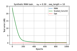
Figure 1: Dynamics of an RNN and its equivalent scaled Conv-1D in learning a synthetic task. the data is generated from a synthetic RNN with $n_{x}=n_{y}=1$ and $nh=4$. Noise is added to the output with SNR$=20$ dB The sequence length T=10. Training and test samples are $N_{\rm tr}=N_{\rm ts}=50$. Full batch gradient descent is used with $lr=10^{-4}$. As you see the dynamics of these models perfectly match.

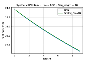
Figure 2: The first 10 epochs in Fig. 1. Note that to be theoretically accurate, we need $lr\rightarrow 0$ to be in the kernel regime.

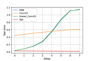
Figure 3: Test performance with respect to delay. For this task we have $n_{h}=1000$, $N_{\rm tr}=N_{\rm ts}=10$, $n_{x}=15$, $n_{y}=1$, and $T=20$. The delay is added manually by shifting i.e. $y_{t}=x_{t}-delay$ and the output SNR = 20 dB.

Given the training and test data, we train (i) a (student) linear RNN with $n=1000$ hidden units, $\nu_{W}=0.3$, and $\nu_{F}=\nu_{C}=1$; and (ii) a 1D-convolutional model with scale coefficients $\rho_{j}$ calculated in (21) using $\nu_{W}=0.3$, $\nu_{F}=\nu_{C}=1$. We used mean-squared error as the loss function for both models and applied full-batch gradient descent with learning rate $lr=10^{-4}$. Fig. 1 shows the identical dynamics of training for both models. Fig. 2 shows a zoomed-in version of the dynamics for training error. Note that the theoretical convergence requires the $lr\rightarrow 0$ and $n\rightarrow\infty$ so that both models operate in the kernel regime.

To evaluate the performance of these models for a task with long-term dependencies, we created a dataset where we manually added different delay steps to the output of a true linear RNN system i.e. $y_{t}=x_{t}-delay$. We have chosen longer ($T=20$) true sequences for this task. We then learned this data using the aforementioned linear RNN and scaled 1D convolutional models. We also trained an unscaled 1D convolutional model with this data to compare performances. With unscaled convolutional model, we exactly learn the impulse response coefficients $L_{j}$ defined in (5) during training.

Fig. 3 shows the test error with respect to delay steps for all three models. Observe that the performance of the scaled convolutional and the linear RNN models match during training. Due to the bias of these models against the delay, the test error increases as we increase the delay steps in our system. On the other hand, the performance of the unscaled convolutional model stays almost the same with increasing delay, slightly changing at larger delays as there is less data to track.

As we increase the delay steps, the test error for these two models increases, and it is due to the fact that these models are biased against the delay.

5.2 Real data

We also validated our theory using spikes rate data from the macaque primary somatosensory cortex (S1) [BFT⁺18]. Somatosensory cortex is a part of the brain responsible for receiving sensations of touch, pain, etc from the entire body. The data is recorded during a two-dimensional reaching task. In this task, a macaque was rewarded for positioning a cursor on a series of randomly generated targets on the screen using a handle. The data is from a single recording of 51 minutes and includes 52 neurons. The mean and median firing rates are $9.3$ and $6.3$ spikes/sec.Similar to the previous experiments, we also trained an unscaled 1D convolutional model with this data and compared the performances with the linear RNN and the scaled convolutional models.

We compared the performances on two sets of experiments. We first used only the 4.5 minutes of the total recorded data. The purpose of this experiment is to compare the performances in limited data circumstances. With this limited data, we expect the scaled convolutional model (and thus the RNN) to perform better than the unscaled model due to the implicit bias of the towards short-term memory and the fact that the effective number of parameters is smaller in the scaled model which leads to a smaller variance. In the second experiment, we trained our models using all the available data ($\approx 51$ mins). In this case, the scaled model (and the RNN) performs worse because of the increased bias error. In our experiments setup, the linear RNN has $n=1000$ hidden states and the sequence length $T=15$. Also, $\nu_{W}=0.3$ and $\nu_{F}=\nu_{C}=1$.

Fig. 4 shows the $R^{2}$ scores for x and y directions of all three models for this task. Observe that, the dynamics of the linear RNN and scaled convolutional model are identical during training using either the entire recording or a part of it. For the case of limited data, as discussed earlier, we observe the implicit bias of the RNN and scaled convolutional model in the figures (a). This bias leads to better performance of these two models compared to the unscaled model. Using the total available data, the unscaled convolutional model performs better because of the increased bias error in the other two models (figures in (b)). Table 1 shows the test $R^{2}$-score of the final trained models for all three cases.

	RNN	Scaled Conv-1D	Conv-1D
$R_{x}^{2}$	0.6462	0.6442	0.6565
$R_{y}^{2}$	0.5911	0.5860	0.6027
$R_{x}^{2}$ (limited data)	0.6043	0.6046	0.5856
$R_{y}^{2}$ (limited data)	0.4257	0.4234	0.3918

Table 1: $R^{2}$-score on test data for x and y directions in the two dimensional reaching task described in section 5.2

(a) Limited data	(b) Entire data

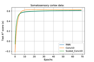
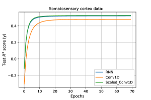
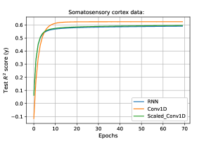
Figure 4: $R^{2}$ score for the two dimensional reaching task described in section 5.2 . The data is recorded from the primary somatosensory cortex of macaques. (a) Limited data: The models are trained on 4.5 minutes of recorded data. (b) Entire data: the whole recording ($\approx 51$ mins) is used to compare the performances. For both cases we used mini-batch (batch size = 128) gradient descent with lr = $10^{-4}$.

6 Conclusion

In this work, we focus on the special class of linear RNNs and observe a functional equivalence between linear RNNs and 1D convolutional models. Using the kernel regime framework, we show that the training of a linear RNN is identical to the training of a certain scaled convolutional model. We further provide an analysis for an inductive bias in linear RNNs towards short-term memory. We show that this bias is driven by the variances of RNN parameters at random initialization. Our theory is validated by both synthetic and real data experiments.

Appendix A Background on Convergence of Vector Sequences and Random Variables

In this section we review some the background on convergence of random variables, definitions of convergence of matrix sequences and some of their properties that we use throughout this paper.

• For a given $p\geq 1$, a function $f:\mathbb{R}^{d}\rightarrow\mathbb{R}^{m}$ is called pseudo-Lipschitz of order $p$, denoted by PL($p$), if

  $$\|f(\mathbf{x}_{1})-f(\mathbf{x}_{2})\|\leq C\|\mathbf{x}_{1}-\mathbf{x}_{2}\|\left(1+\|\mathbf{x}_{1}\|^{p-1}+\|\mathbf{x}_{2}\|^{p-1}\right)$$ (26)

  for some constant $C>0$.

This is a generalization of the standard definition of Lipshitiz continuity. A PL(1) function is Lipschitz with constant $3C$.

• Consider a sequence of vectors $\mathbf{x}(N)=\{\mathbf{x}_{n}{(N)}\}_{n=1}^{N}$ with $\mathbf{x}_{n}(N)\in\mathbb{R}^{d}$. So, each $\mathbf{x}(N)$ is a block vector with a total of $Nd$ components. For a finite $p\geq 1$, we say that the vector sequence $\mathbf{x}(N)$ converges empirically with $p$-th order moments if there exists a random variable $X\in\mathbb{R}^{d}$ such that

  1. $\mathbb{E}\|X\|_{p}^{p}<\infty$; and

  2. for any $f:\mathbb{R}^{d}\rightarrow\mathbb{R}$ that is pseudo-Lipschitz continuous of order $p$,

     $$\lim_{N\rightarrow\infty}\frac{1}{N}\sum_{n=1}^{N}f(\mathbf{x}_{n}(N))=\mathbb{E}\left[f(X)\right].$$ (27)

In this case, with some abuse of notation, we will write

$$\lim_{n\rightarrow\infty}\mathbf{x}_{n}\stackrel{{\scriptstyle PL(p)}}{{=}}X,$$ (28)

where we have omitted the dependence on $N$ in $\mathbf{x}_{n}(N)$. We note that the sequence $\{\mathbf{x}{(N)}\}$ can be random or deterministic. If it is random, we will require that for every pseudo-Lipschitz function $f(\cdot)$, the limit (27) holds almost surely. In particular, if $\mathbf{x}_{n}\sim X$ are i.i.d. and $\mathbb{E}\|X\|^{p}_{p}<\infty$, then $\mathbf{x}$ empirically converges to $X$ with $p^{\rm th}$ order moments.

Weak convergence (or convergence in distribution) of random variables is equivalent to

$$\lim_{n\rightarrow\infty}\mathbb{E}f(X_{n})=\mathbb{E}f(X),\quad\text{for all bounded functions }f.$$ (29)

It is shown in [BM11] that PL$(p)$ convergence is equivalent to weak convergence plus convergence in $p$ moment.

• Let $\nu$ and $\mu$ be two distributions on some Euclidean space $\mathcal{X}$. The Wasserstein-2 distance between $\nu$ and $\mu$ is defined as

  $$W_{2}(\nu,\mu)=\left(\inf_{\gamma\in\Gamma}\mathbb{E}\|X-X^{\prime}\|_{2}^{2}\right)^{\frac{1}{2}},$$ (30)

  where $\Gamma$ is the set of all distributions with marginals consistent with $\nu$ and $\mu$.

A sequence $x_{n}$ converges PL(2) to $X$ if and only if the empirical measure $\hat{\mathbb{P}}_{N}=\frac{1}{N}\sum_{n=1}^{N}\delta(x-x_{n})$ (where $\delta(\cdot)$ is the Dirac measure,) converges in Wasserstein-2 distance to distribution of $X$ [Vil08], i.e.

$$x_{n}\stackrel{{\scriptstyle PL(2)}}{{=}}X\quad\iff\quad\lim_{n\rightarrow\infty}W_{2}(\hat{\mathbb{P}}_{N},\mathbb{P}_{X})=0.$$ (31)

For two zero mean Gaussian measure $\nu=\mathcal{N}(0,\Sigma_{1}),\mu=\mathcal{N}(0,\Sigma_{2})$ the Wasserstein-2 distance is given by [GS⁺84]

$$W^{2}_{2}(\nu,\mu)=\mathrm{tr}(\Sigma_{1}-2(\Sigma_{1}^{1/2}\Sigma_{2}\Sigma_{1}^{1/2})^{1/2}+\Sigma_{2}).$$ (32)

Therefore, for zero mean Gaussian measures, convergence in covariance, implies convergence in Wasserstein-2 distance, and hence if the empirical covariance of a zero mean Gaussian sequence $x_{n}$ converges to some covaraince matrix $\Sigma$, then using (31) $x_{n}\stackrel{{\scriptstyle PL(2)}}{{=}}X$ where $X\sim\mathcal{N}(0,\Sigma)$.

Appendix B Proofs

B.1 Proof of Proposition 2.1

Suppose we are given a convolutional model (5) with impulse response coefficients $L_{t}$, $t=0,\ldots,T-1$. It is well-known from linear systems theory [Kai80] that linear time-invariant systems are input-output equivalent if and only if they have the same impulse response coefficients. So, we simply need to find matrices $(W,F,C)$ satisfying (9). First consider the single input single output (SISO) case where $n_{x}=n_{y}=1$. Take any set of real non-zero scalars $\lambda_{i}$, $i=0,\ldots,T-1$, that are distinct and set

$$W=\mathrm{diag}(\lambda_{0},\ldots,\lambda_{T-1}),\quad F=1_{T},$$ (33)

so there are $n=T$ hidden states. Then, for any $t$,

$$(CW^{t}F)=\sum_{k=0}^{T-1}C_{k}\lambda_{k}^{t}.$$ (34)

Equivalently, the impulse response coefficients in (9) are given by,

$$[L_{0},\cdots,L_{T-1}]=CV,$$ (35)

where $V$ is the Vandermode matrix $V_{jt}=\lambda_{j}^{t}$. Since the values $\lambda_{j}$ are distinct, $V$ is invertible and we can find a vector $C$ matching arbitrary impulse response coefficients. Thus, when $n_{x}=n_{y}=1$, we can find a linear RNN with at most $n=T$ hidden states that match the first $T$ impulse response coefficients. To extend to the case of arbitrary $n_{x}$ and $n_{y}$, we simply create $n_{x}n_{y}$ systems, one for each input-output component pair. Since each system will have $T$ hidden states, the total number of states would be $n=Tn_{x}n_{y}$.

B.2 Proof of Theorem 3.2

Given $y_{t}=\sum_{j=0}^{t}\sqrt{\rho_{j}}\theta_{j}x_{t-j}$ and $\theta=(\theta_{0},\dots,\theta_{T-1})$, we consider a perturbation in $\theta$, namely $\Delta_{\theta}$. Therefore,

$$\widetilde{y}_{t}=\sum_{j=0}^{t}\sqrt{\rho_{j}}{\Delta_{\theta}}_{j}x_{t-j}$$ (36)

and the NTK for this model is given by

$$K_{t,s}(x,x^{\prime})=\sum_{\Delta_{\theta}\in T_{\theta}}\widetilde{y}_{t}(\Delta_{\theta})\widetilde{y}_{s}^{\prime}(\Delta_{\theta})^{\text{\sf T}}.$$ (37)

where $T_{\theta}$ is the standard basis for the parameter space. The following lemma shows this sum can be calculated as an expectation over a Gaussian random variable.

Lemma B.1.

Let $V$ be a finite dimensional Hilbert space and $W=\mathbb{R}^{m}$ with the standard inner product and let $T,T^{\prime}:V\rightarrow W$ be linear transformations. Let $\{v_{i}\}_{i=1}^{n}$ be an ordered orthonormal basis for V. Then we have

$$\sum_{i=1}^{n}T(v_{i})(T^{\prime}(v_{i}))^{\text{\sf T}}=\mathbb{E}_{\alpha\sim\mathcal{N}(0,I_{n})}\left[T\big{(}\sum_{i=1}^{n}\alpha_{i}v_{i}\big{)}\bigg{(}T^{\prime}\big{(}\sum_{i=1}^{n}\alpha_{i}v_{i}\big{)}\bigg{)}^{\text{\sf T}}\right].$$ (38)

Proof.

$$\mathbb{E}_{\alpha\sim\mathcal{N}(0,I_{n})}\left[T\big{(}\sum_{i=1}^{n}\alpha_{i}v_{i}\big{)}\bigg{(}T^{\prime}\big{(}\sum_{j=1}^{n}\alpha_{j}v_{j}\big{)}\bigg{)}^{\text{\sf T}}\right] =\mathbb{E}_{\alpha\sim\mathcal{N}(0,I_{n})}\left[\sum_{i,j=1}^{n}\alpha_{i}\alpha_{j}T\big{(}v_{i}\big{)}T^{\prime}\big{(}v_{j}\big{)}^{\text{\sf T}}\right]$$

$$=\sum_{i=1}^{n}T(v_{i})(T^{\prime}(v_{i}))^{\text{\sf T}}.$$ (39)

∎

Since $\widetilde{y}_{t}(\Delta_{\theta})$ is a linear operator, by applying Lemma B.1 we have,

$$K_{t,s}(x,x^{\prime}) =\mathbb{E}_{\Delta_{\theta}\sim\mathcal{N}(0,1),\text{i.i.d.}}\ [\widetilde{y}_{t}(\Delta_{\theta})\widetilde{y}_{s}^{\prime}(\Delta_{\theta})^{\text{\sf T}}]$$

$$=\mathbb{E}_{\Delta_{\theta}\sim\mathcal{N}(0,1),\text{i.i.d.}}\ \left[(\sum_{j=0}^{t}\sqrt{\rho_{j}}{\Delta_{\theta}}_{j}x_{t-j})(\sum_{k=0}^{t}\sqrt{\rho_{k}}{\Delta_{\theta}}_{k}x^{\prime}_{s-k})^{\text{\sf T}}\right]$$

$$=\mathbb{E}_{\Delta_{\theta}\sim\mathcal{N}(0,1),\text{i.i.d.}}\ \left[(\sum_{j=0}^{t}\rho_{j}\ {\Delta_{\theta}}_{j}x_{t-j}{x^{\prime}_{s-j}}^{\text{\sf T}}{\Delta_{\theta}}_{j}^{\text{\sf T}})\right]$$

Therefore,

$$\bigg{(}K_{t,s}(x,x^{\prime})\bigg{)}_{m,m^{\prime}} =\mathbb{E}_{\Delta_{\theta}\sim\mathcal{N}(0,1),\text{i.i.d.}}\ \left[\sum_{j=0}^{t}\rho_{j}\ \sum_{k,k^{\prime}}{({\Delta_{\theta}}_{j})}_{m,k}x_{t-j,k}{x^{\prime}_{s-j,k^{\prime}}}{({\Delta_{\theta}}_{j})}_{k^{\prime},m^{\prime}}\right]$$

$$=(\sum_{j=0}^{t}\rho_{j}\ x_{t-j}^{\text{\sf T}}x^{\prime}_{s-j})\delta_{m,m^{\prime}}$$

Thus, $K_{t,s}(x,x^{\prime})=(\sum_{j=0}^{t}\rho_{j}\ x_{t-j}^{\text{\sf T}}x^{\prime}_{s-j})I_{n_{y}}$ and we can write the full kernel as

$$K(x,x^{\prime})=\mathcal{T}(x)^{\text{\sf T}}D(\rho)\mathcal{T}(x^{\prime})\otimes I_{n_{y}},$$ (40)

where $\mathcal{T}(x)$ and $D(\rho)$ are defined in (18) and (19) respectively.

B.3 Proof of Theorem 3.3

Part (a) is a special case of a more general lemma, Lemma C.1 which we present in Appendix C. Let

$$q_{t+1}=\frac{1}{\sqrt{n}}Wq_{t},\quad q_{0}=F,$$ (41)

so that $q_{t}$ represents the impulse response from $x_{t}$ to $h_{t}$. That is,

$$h_{t}=\sum_{j=0}^{t}q_{t-j}x_{j},$$ (42)

which is the convolution of $q_{t}$ and $h_{t}$. The system (41) is a special case of (68) with $L=1$, no input $u_{t}$ and

$$A=W,\quad G(q)=q.$$

Since there is only $L=1$ transform, we have dropped the dependence on the index $\ell$. Lemma C.1 hows that $(q_{0},\ldots,q_{t})$ converges $PL(2)$ to a Gaussian vector $(Q_{0},\ldots,Q_{t})$ with zero mean. We claim that the $Q_{i}$’s are independent. We prove this with induction. Suppose $(Q_{0},\ldots,Q_{t})$ are independent. We need to show $(Q_{0},\ldots,Q_{t+1})$ are independent by using the SE equations (72). Specifically, from (72b), $Z_{i}=Q_{i}$ for all $i$. Also, since each $Q_{i}$ is zero mean, $\mu_{i}=0$ and $\widetilde{Z}_{i}=Z_{i}=Q_{i}$. Since the $\widetilde{Z}_{i}$ are independent, the linear predictor coefficients in (72d) are zero: $F_{ti}=0$. Therefore, $\widetilde{R}_{t}=R_{t}\sim\mathcal{N}(0,\nu_{W}P_{t})$ is independent of $(R_{0},\ldots,R_{t-1})$. From (72h), $Q_{t+1}=R_{t}$. So, we have that $(Q_{0},\ldots,Q_{t-1})$ is an independent Gaussian vector. Finally, to compute the variance of the $Q_{t+1}$, observe

$${\rm cov}(Q_{t+1}) \stackrel{{\scriptstyle(a)}}{{=}}{\rm cov}(R_{t})\stackrel{{\scriptstyle(b)}}{{=}}\nu_{W}P_{t}$$

$$\stackrel{{\scriptstyle(c)}}{{=}}\nu_{W}{\rm cov}(Z_{t})\stackrel{{\scriptstyle(d)}}{{=}}\nu_{W}{\rm cov}(Q_{t}),$$ (43)

where (a) follows from (72h); (b) follows from (72f) and the fact that $F_{ti}=0$ for all $i$; (c) follows from (72e); and (d) follows from the fact that $Z_{t}=Q_{t}$. Also, since $q_{0}=F$, it follows that $Q_{0}\sim\mathcal{N}(0,\nu_{F}I)$. We conclude that ${\rm cov}(Q_{t})=\nu_{F}\nu_{W}^{t}I_{n_{x}}$. This proves part (a).

For part (b), we consider perturbations $\Delta_{W}$, $\Delta_{F}$, and $\Delta_{C}$ of the parameters $W$, $F$, and $C$. We have that,

$$\widetilde{h}_{t}=\frac{1}{\sqrt{n}}W\widetilde{h}_{t-1}+\frac{1}{\sqrt{n}}\Delta_{W}h_{t}+\Delta_{F}x_{t},\qquad\widetilde{y}_{t}=\frac{1}{\sqrt{n}}C\widetilde{h}_{t}+\Delta_{C}h_{t}$$ (44)

Combining this equation with (1), we see that the mapping from $x_{t}$ to $[h_{t}~{}\widetilde{h}_{t}]$ is a linear time-invariant system. Let $q_{t}\in\mathbb{R}^{n\times 2n_{x}}$ be its impulse response. The impulse response coefficients satisfy the recursive equations,

$$q_{t+1}=\left[\frac{1}{\sqrt{n}}Wq_{t,1},\frac{1}{\sqrt{n}}(Wq_{t,2}+\Delta_{W}q_{t,1})\right],\quad q_{0}=\left[F,\Delta_{F}\right].$$

We can analyze these coefficients in the LSL using Lemma C.1. Specifically, let $L=2$ and set

$$A_{1}=W,\quad A_{2}=\Delta_{W}.$$

Also, let

$$z_{t1} =\overline{G}_{1}(q_{t}):=q_{t},$$ (45a)

$$z_{t2} =\overline{G}_{2}(q_{t}):=[0\ ~{}q_{t1}].$$ (45b)

Then, we have the updates,

$$q_{t+1}=\frac{1}{\sqrt{n}}Wz_{t1}+\frac{1}{\sqrt{n}}\Delta_{W}z_{t2},\quad q_{0}=\left[F,\Delta_{F}\right].$$

It follows from Lemma C.1 that $(q_{0},\ldots,q_{T-1})$ converges $PL(2)$ to zero mean Gaussian random variables $(Q_{0},\ldots,Q_{T-1})$. Note that $Q_{t}=[Q_{t1},Q_{t2}]$ where each $Q_{t1}$ and $Q_{t2}$ are random vectors $\in\mathbb{R}^{1\times n_{x}}$.

Similar to the proof of the previous theorem, we use induction to show that $(Q_{0},\ldots,Q_{t})$ are independent. Suppose that the claim is true for $t$. Then, $Z_{i1}$ and $Z_{i2}$ are functions of $Q_{i}$. So, for $\ell=1,2$, $Z_{t\ell}$ is independent of $Z_{i\ell}$ for $i<t$. Thus, the prediction coefficients $F_{ti\ell}=0$ and, as before, $R_{t\ell}\sim\mathcal{N}(0,P_{t\ell})$ independent of $R_{i\ell}$, $i<t$. Thus, $Q_{t+1}=R_{t1}+R_{t2}$ is independent of $(Q_{0},\ldots,Q_{t})$.

We conclude by computing the ${\rm cov}(Q_{t})$. We claim that, for all $t$, the variance of $Q_{t}$ is of the form,

$${\rm cov}(Q_{t})=\left[\begin{array}[]{cc}\tau_{t1}I_{n_{x}}&0\\ 0&\tau_{t2}I_{n_{x}}\end{array}\right]$$ (46)

for scalar $\tau_{t1},\tau_{t2}$. Since $q_{0}=\left[F,\Delta_{F}\right]$, we have

$$\tau_{t1}=\nu_{F},\quad\tau_{t2}=1.$$

Now suppose that (46) is true for some $t$. From (72b),

$$Z_{t1}=Q_{t},\quad Z_{t1}=(0,Q_{t1}),$$

from which we obtain that

$${\rm cov}(Z_{t1})=\left[\begin{array}[]{cc}\tau_{t1}I_{n_{x}}&0\\ 0&\tau_{t2}I_{n_{x}}\end{array}\right],\quad{\rm cov}(Z_{t2})=\left[\begin{array}[]{cc}0&0\\ 0&\tau_{t1}I_{n_{x}}\end{array}\right].$$ (47)

Therefore, we have

$${\rm cov}(Q_{t+1}) \stackrel{{\scriptstyle(a)}}{{=}}{\rm cov}(R_{t,1})+{\rm cov}(R_{t,2})$$

$$\stackrel{{\scriptstyle(b)}}{{=}}\nu_{W}P_{t1}+P_{t2}$$

$$\stackrel{{\scriptstyle(c)}}{{=}}\nu_{W}{\rm cov}(Z_{t1})+{\rm cov}(Z_{t2})\stackrel{{\scriptstyle(d)}}{{=}}\left[\begin{array}[]{cc}\nu_{W}\tau_{t1}I_{n_{x}}&0\\ 0&(\tau_{t1}+\nu_{W}\tau_{t2})I_{n_{x}}\end{array}\right],$$ (50)

where (a) follows from (72h); (b) follows from (72f) and the fact that $F_{ti\ell}=0$ for all $i$; (c) follows from (72e); and (d) follows from (47). It follows that

$$\tau_{t+1,1}=\nu_{W}\tau_{t1},\quad\tau_{t+1,2}=\nu_{W}\tau_{t2}+\tau_{t1}.$$

These recursions have the solution,

$$\tau_{t1}=\nu_{W}^{t}\nu_{F},\quad\tau_{t2}=t\nu_{F}\nu_{W}^{t-1}+\nu_{W}^{t}.$$ (51)

Since $[h_{t},\widetilde{h}_{t}]=\sum_{j=0}^{t}q_{j}\begin{bmatrix}x_{t-j}\\ x_{t-j}\end{bmatrix}$ and we know each $q_{t}$ converges $PL(2)$ to random $Q_{t}$ with covariances calculated in (46) and (51), we have

$$[h_{t},\widetilde{h}_{t}]\stackrel{{\scriptstyle PL(2)}}{{=}}[H_{t},\widetilde{H}_{t}]=\sum_{j=0}^{t}Q_{j}\begin{bmatrix}x_{t-j}\\ x_{t-j}\end{bmatrix}$$ (52)

where $H_{t},\widetilde{H}_{t}$ are scalar random variables. For each $t,s$, we can now calculate the auto-correlation function for $H$ as follows

$$\mathbb{E}[H_{t}H_{s}] =\mathbb{E}[\sum_{j=0}^{t}\sum_{k=0}^{t}x_{t-j}^{\text{\sf T}}Q_{j,1}^{\text{\sf T}}Q_{k,1}x_{s-k}]$$

$$=\sum_{j=0}^{t}x_{t-j}^{\text{\sf T}}\mathbb{E}[Q_{j,1}^{\text{\sf T}}Q_{j,1}]x_{s-j}$$

$$=\sum_{j=0}^{t}\nu_{W}^{j}\nu_{F}\ x_{t-j}^{\text{\sf T}}x_{s-j}.$$ (53)

Similarly for $\widetilde{H}$ we have

$$\mathbb{E}[\widetilde{H}_{t}\widetilde{H}_{s}]=\sum_{j=0}^{t}\ (j\nu_{F}\nu_{W}^{j-1}+\nu_{W}^{j})\ x_{t-j}^{\text{\sf T}}x_{s-j}.$$ (54)

Thus, the impulse response of the system $L_{j}=Cq_{j,1}$ converge empirically to $\mathcal{N}(0,\Lambda)$ where,

$$\Lambda=\nu_{C}\lim_{n\rightarrow\infty}\frac{1}{n}q_{j,1}^{\text{\sf T}}q_{j,1}=\nu_{C}\mathbb{E}[Q_{j,1}^{\text{\sf T}}Q_{j,1}]=\nu_{C}\nu_{F}\nu_{W}^{j}I_{n_{x}}.$$ (55)

This proves part (a).

Note that $\mathbb{E}[\widetilde{H}_{t}\widetilde{H}^{\prime}_{s}]$ and $\mathbb{E}[H_{t}H^{\prime}_{s}]$ can be calculated similarly by substituting $x_{s-j}$ with $x^{\prime}_{s-j}$ in (B.3) and (54).

Next, we calculate the NTK in this case

$$K_{t,s}(x,x^{\prime}) =\sum_{\Delta_{\Theta}\in T_{\Theta}}\widetilde{y}_{t}(\Delta_{\Theta})\widetilde{y}_{s}^{\prime}(\Delta_{\Theta})^{\text{\sf T}}$$

$$\stackrel{{\scriptstyle(a)}}{{=}}\mathbb{E}_{\Delta_{\Theta}\sim\mathcal{N}(0,1),\text{i.i.d.}}\ [\widetilde{y}_{t}(\Delta_{\Theta})\widetilde{y}_{s}^{\prime}(\Delta_{\Theta})^{\text{\sf T}}]$$ (56)

where (a) follows from Lemma B.1. Combining with (44) we have

$$K_{t,s}(x,x^{\prime}) =\mathbb{E}_{C,\Delta_{C}\sim\mathcal{N}(0,1),\text{i.i.d.}}\ \left[(C\widetilde{h}_{t}+\Delta_{C}h_{t})(C\widetilde{h}^{\prime}_{s}+\Delta_{C}h_{s}^{\prime})^{\text{\sf T}}\right]$$

$$=\left(\nu_{C}\mathbb{E}[\widetilde{H}_{t}\widetilde{H}^{\prime}_{s}]+\mathbb{E}[H_{t}H^{\prime}_{s}]\right)I_{n_{y}}$$ (57)

Therefore,

$$K(x,x^{\prime})=\mathcal{T}(x)^{\text{\sf T}}D(\rho)\mathcal{T}(x^{\prime})\otimes I_{n_{y}},$$ (58)

where $\mathcal{T}(x)$ and $D(\rho)$ are given in (18) and (19) and

$$\rho_{i}=\nu_{C}(i\nu_{F}\nu_{W}^{i-1}+\nu_{W}^{i})+\nu_{W}^{i}\nu_{F}.$$ (59)

This proves part (b).

B.4 Proof of Theorem 4.1

Bounding the Initial Impulse Response

from Theorem 3.3, each coefficient of $L_{{\rm RNN},j}^{0}$ has mean zero and variance $\nu_{C}\nu_{F}\nu_{W}^{j}$. There are $n_{x}n_{y}$ such components. This proves (24).

Convolutional Equivalent Linear Model

The key for the remainder of the proof is to use Theorems 3.2 and 3.3 to construct a scaled convolutional model that has the same NTK and intial conditions as the RNN. Then, we analyze the convolutional model to obtain the desired bound. To this end, let $\mathbb{\rho}=[\rho_{0},\ldots,\rho_{T-1}]$ be the scaling factors given in Theorem 3.3. For each initial condition $\theta^{0}_{\rm RNN}=(W^{0},F^{0},C^{0})$ of the RNN, suppose that we initialize the scaled convolutional model with

$$\theta_{{\rm conv},j}^{0}=\frac{1}{\sqrt{\rho_{j}}n^{(j+1)/2}}C^{0}(W^{0})^{j}F^{0}.$$

The initial impulse response of the scaled convolutional model will then be

$$L_{{\rm conv},j}^{0}=\sqrt{\rho_{j}}\theta_{{\rm conv},j}=\frac{1}{n^{(j+1)/2}}C^{0}(W^{0})^{j}F^{0}=L_{{\rm RNN},j}^{0}.$$ (60)

Hence, the scaled convolutional model and the RNN have the same initial impulse response coefficients. We then train the scaled convolutional model on the training data using gradient descent with the same learning rate $\eta$ used in the training of the RNN. Let $L_{{\rm conv},j}^{\ell}$ denote the impulse response of the scaled convolutional model after $\ell$ steps of gradient descent.

Gradient Descent Analysis of the Convolutional Model

Next, we look at how the impulse response of the scaled convolutional model evolves over the gradient descent steps. It is convenient to do this analysis using some matrix notation. For each parameter, $\theta=[\theta_{0},\ldots,\theta_{T-1}]$, the convolutional filter parameters are $L_{j}=\sqrt{\rho_{j}}\theta_{j}$. Thus, we can write

$$\mathbf{L}=\mathbf{D}^{1/2}\theta,$$

where $\mathbf{D}$ is a block diagonal operator with values $\rho_{j}$. Also, let $\widehat{\mathbf{y}}=[\widehat{\mathbf{y}}_{1},\ldots,\widehat{\mathbf{y}}_{N}]$ be the set of predictions on the $N$ training samples. Since the convolutional model is linear, we can write $\hat{\mathbf{y}}=\mathbf{A}\mathbf{L}$ for some linear operator $\mathbf{A}$. The operator $\mathbf{A}$ would be a block Toeplitz with the input data $\mathbf{x}=[\mathbf{x}_{1},\ldots,\mathbf{x}_{N}]$. Also, if we let $\mathbf{y}=[\mathbf{y}_{1},\ldots,\mathbf{y}_{N}]$ be the $N$ training samples, the least squares cost is

$$\|\mathbf{y}-\mathbf{A}\mathbf{D}^{1/2}\mathbf{\theta}\|^{2}_{F}.$$

Minimizing this loss function will result in GD steps,

$$\theta^{\ell+1}=\theta^{\ell}+\eta\mathbf{D}^{1/2}\mathbf{A}^{\text{\sf T}}(\mathbf{y}-\mathbf{A}\mathbf{D}^{1/2}\theta^{\ell}).$$

Now let $\mathbf{u}^{\ell}=\mathbf{D}^{-1/2}(\mathbf{\theta}^{\ell}-\mathbf{\theta}^{0})$ and $\mathbf{b}:=\mathbf{y}-\mathbf{A}\mathbf{D}^{1/2}\mathbf{\theta}^{0}$. Then,

$$\mathbf{u}^{\ell+1}=\mathbf{u}^{\ell}+\eta\mathbf{A}^{\text{\sf T}}(\mathbf{b}-\mathbf{A}\mathbf{D})\mathbf{u}^{\ell}=(\operatorname*{\mathbf{I}}-\eta\mathbf{A}^{\text{\sf T}}\mathbf{A}\mathbf{D})\mathbf{u}^{\ell}+\eta\mathbf{A}^{\text{\sf T}}\mathbf{b}$$ (61)

For $0<\nu_{W}<1$, we have that $\rho_{j}$ satisfies the bound (22). Since $\mathbf{D}$ is a block diagonal matrix with entries $\rho_{j}$, $\|\mathbf{D}\|\leq\rho_{\rm max}$. Now select

$$B_{1}:=\frac{1}{\rho_{\rm max}\|\mathbf{A}\|^{2}},\quad B_{2}:=\|\mathbf{A}^{\text{\sf T}}\mathbf{b}\|.$$ (62)

If we take $\eta<B_{1}$ then

$$\eta\mathbf{D}^{1/2}\mathbf{A}^{\text{\sf T}}\mathbf{A}\mathbf{D}^{1/2}\leq\eta\rho_{\rm max}\|\mathbf{A}\|^{2}\leq\operatorname*{\mathbf{I}}\Rightarrow\|\mathbf{I}-\eta\mathbf{A}^{\text{\sf T}}\mathbf{A}\mathbf{D}\|\leq 1.$$

Hence, (61) shows that

$$\|\mathbf{u}^{\ell+1}\|_{F}\leq\|\mathbf{u}^{\ell}\|_{F}+\eta B_{2}\Rightarrow\|\mathbf{u}^{\ell}\|_{F}\leq\eta\ell B_{2},$$ (63)

where we have used the fact that $\mathbf{u}^{0}=\mathbf{0}$. Now, since $\mathbf{u}^{\ell}=\mathbf{D}^{-1/2}(\mathbf{\theta}^{\ell}-\mathbf{\theta}^{0})$, the $j$-th component of $\mathbf{\theta}^{\ell}$ is

$$\mathbf{\theta}^{\ell}_{j}=\mathbf{\theta}^{0}_{j}+\sqrt{\rho_{j}}\mathbf{u}^{\ell}_{j}.$$

Hence,

$$L_{{\rm conv},j}^{\ell} =\sqrt{\rho_{j}}\theta_{j}^{\ell}=L_{{\rm conv},j}^{0}+\rho_{j}\mathbf{u}^{\ell}_{j}.$$

Applying (63) we obtain the bound on the convolutional model

$$\|L_{{\rm conv},j}^{\ell}-L_{{\rm conv},j}^{0}\|_{F}\leq\rho_{j}\eta\ell B_{2}.$$ (64)

Bounding the RNN Impulse Response

From Theorems 3.2 and 3.3, the scaled convolutional model and linear RNN have the same NTK. Due to (60), they have the same input-output mapping at the initial conditions. Since the scaled convolutional model is linear in its parameters it follows that it is linear NTK model for the RNN. Therefore, using the NTK results such as Proposition 3.1, we have that for all input sequences $\mathbf{x}$ and GD time steps $\ell$,

$$\lim_{n\rightarrow\infty}\left\|f_{\rm RNN}(\mathbf{x},\theta^{\ell}_{\rm RNN})-f_{\rm conv}(\mathbf{x},\theta^{\ell}_{\rm conv})\right\|=0,$$ (65)

where the convergence is in probability. Thus, if we fix an input $\mathbf{x}$ and iteration $\ell$ and define

$$\mathbf{y}_{\rm RNN}=f_{\rm RNN}(\mathbf{x},\theta_{\rm RNN}^{\ell}),\quad\mathbf{y}_{\rm conv}=f_{\rm conv}(\mathbf{x},\theta_{\rm conv}^{\ell}),$$

the limit (65) can be re-written as

$$\lim_{n\rightarrow\infty}\left\|y_{{\rm RNN},j}-y_{{\rm conv},j}\right\|=0,$$ (66)

for all $j$. Again, the convergence is in probability. Now consider the case where the input sequence $\mathbf{x}=(x_{0},\ldots,x_{T-1})$ is a sequence with $x_{j}=0$ for all $j>0$ That is, it is only non-zero at the initial time step. Then for all time steps $y_{{\rm RNN},j}=L_{{\rm RNN},j}^{\ell}x_{0}$ and $y_{{\rm conv},j}=L_{{\rm conv},j}^{\ell}x_{0}$. Since this is true for all $x_{0}$, (66) shows that for all time steps $j=0,\ldots,T-1$,

$$\lim_{n\rightarrow\infty}\left\|L_{{\rm RNN},j}(x,\theta^{\ell}_{\rm RNN})-L_{{\rm conv},j}(x,\theta^{\ell}_{\rm conv})\right\|_{F}=0$$ (67)

where the convergence is in probability. Combining (67) with (64) proves (25).

Appendix C Recursions with Random Gaussians

We consider a recursion of the form,

$$q_{t+1}=\sum_{\ell=1}^{L}\frac{1}{\sqrt{n}}A_{\ell}\overline{G}_{\ell}(q_{t},u_{t}),$$ (68)

where $q_{t}\in\mathbb{R}^{n\times d_{q}}$, $u_{t}\in\mathbb{R}^{n\times d_{u}}$, and $\overline{G}_{\ell}(q_{t},u_{t})$ acts row-wise, meaning

$$\overline{G}_{\ell}(q_{t},u_{t})_{i,:}=G_{\ell}(q_{t,i,:},u_{t,i,:}),$$ (69)

for some Lipschitz functions $G_{\ell}:\mathbb{R}^{d_{q}}\times\mathbb{R}^{d_{u}}\times\rightarrow\mathbb{R}^{d_{q}}$. That is, the outptut of row $i$ of $\overline{G}_{\ell}(\cdot)$ depends only the $i$-th rows of its inputs. We will analyze this system for a fixed horizon, $t=0,\ldots,T-1$. Assume that

$$(q_{0},u_{0},\ldots,u_{T-1})\stackrel{{\scriptstyle PL(2)}}{{\rightarrow}}(Q_{0},U_{0},\ldots,U_{T-1}),$$ (70)

to random variables $(Q_{0},U_{0},\ldots,U_{T-1})$ where $Q_{0}$ is independent of $(U_{0},\ldots,U_{T-1})$, and $Q_{0}\sim\mathcal{N}(0,P_{0})$ for some covariance matrix $P_{0}\in\mathbb{R}^{d_{q}\times d_{q}}$. Assume the matrices $A_{\ell}\in\mathbb{R}^{n\times n}$ are independent with i.i.d. components, $(A_{\ell})_{i,j}\sim\mathcal{N}(0,\nu_{\ell})$.

Lemma C.1.

Under the above assumptions,

$$(q_{0},q_{1},\dots,q_{T-1},u_{0},u_{1},\dots,u_{T-1})\stackrel{{\scriptstyle PL(2)}}{{\rightarrow}}(Q_{0},Q_{1},\dots,Q_{T-1},U_{0},\dots U_{T-1})$$ (71)

where each $Q_{i}\in\mathbb{R}^{d_{q}}$ and $(Q_{0},Q_{1},\dots,Q_{T-1})$ are zero mean Gaussian processes independent of $(U_{0},\dots U_{T-1})$, generated recursively through SE equations given by

$$D_{\ell} ={\mathcal{N}}(0,\nu_{\ell})$$ (72a)

$$Z_{t\ell} =G_{\ell}(Q_{t},U_{t})$$ (72b)

$$\mu_{t\ell} =\mathbb{E}(Z_{t\ell}),\quad\tilde{Z}_{t\ell}=Z_{t\ell}-\mu_{t\ell}$$ (72c)

$$F_{t,:,\ell} =\min_{F_{1},\ldots,F_{t-1}}\mathbb{E}\left\|\tilde{Z}_{t\ell}-\sum_{j=1}^{t}\tilde{Z}_{t-j,\ell}F_{j}\right\|^{2}$$ (72d)

$$P_{t\ell} =\mathbb{E}(\tilde{Z}_{t\ell}-\sum_{j=1}^{t}\tilde{Z}_{t-j,\ell}F_{tj\ell})^{\text{\sf T}}(\tilde{Z}_{t\ell}-\sum_{j=1}^{t}\tilde{Z}_{t-j,\ell}F_{tj\ell})$$ (72e)

$$\tilde{R}_{t\ell} =\sum_{j=1}^{t}\tilde{R}_{t-j,\ell}F_{tj\ell}+{\mathcal{N}}(0,\nu_{W}P_{t\ell}),$$ (72f)

$$R_{t\ell} =\tilde{R}_{t\ell}+D_{\ell}\mu_{t\ell}$$ (72g)

$$\quad Q_{t+1} =\sum_{\ell=1}^{L}R_{t\ell}$$ (72h)

Proof:

We prove this by induction. Let $\mathcal{M}_{t}$ be the hypothesis that this result is true up to iteration $t$. We show that $\mathcal{M}_{0}$ is true and that $\mathcal{M}_{t}$ implies $\mathcal{M}_{t+1}$.

Base case ($\mathcal{M}_{0}$):

Define $z_{0\ell}=\overline{G}_{\ell}(q_{0},u_{0})$. We have that rows of $z_{0\ell}$ converge $PL(2)$ to $Z_{0\ell}=\overline{G}_{\ell}(Q_{0},U_{0})$.

Now, let $\mu_{0\ell}=\mathbb{E}(Z_{0\ell})$ and define the following:

$$d_{\ell} =\frac{1}{\sqrt{n}}A_{\ell}\mathbf{1},\quad\widetilde{z}_{0\ell}=z_{0\ell}-\mathbf{1}\mu_{0\ell}$$ (73)

$$\widetilde{r}_{1\ell} =\frac{1}{\sqrt{n}}A_{\ell}\widetilde{z}_{0\ell},\quad r_{1\ell}=\widetilde{r}_{1\ell}+d_{\ell}\mu_{0\ell},\quad q_{1}=\sum_{\ell=1}^{L}r_{1\ell}.$$ (74)

We know that

$$d_{\ell}\stackrel{{\scriptstyle PL(2)}}{{=}}D_{\ell}\sim\mathcal{N}(0,\nu_{\ell}),\qquad\widetilde{z}_{0\ell}\stackrel{{\scriptstyle PL(2)}}{{=}}\widetilde{Z}_{0\ell}=Z_{0\ell}-\mu_{0\ell}.$$ (75)

Note that $\widetilde{Z}_{0\ell}$ are zero mean. Now since $A_{\ell}$ are i.i.d Gaussian matrices, rows of $\widetilde{r}_{1\ell}$ converge PL(2) to random variable

$$\widetilde{R}_{1\ell}\sim\mathcal{N}(0,P_{1\ell})\qquad\text{where, }\quad P_{1\ell}=\lim_{n\rightarrow\infty}\frac{1}{n}{\widetilde{z}_{0\ell}}^{\text{\sf T}}\widetilde{z}_{0\ell}\stackrel{{\scriptstyle a.s.}}{{=}}\mathbb{E}(\widetilde{Z}_{0\ell}^{\text{\sf T}}\widetilde{Z}_{0\ell})$$ (76)

Furthermore, one can show that $\mathbb{E}(\widetilde{R}_{1\ell_{1}}\widetilde{R}_{1\ell_{2}})=\mathbb{E}(\widetilde{Z}_{0\ell_{1}}^{\text{\sf T}}\widetilde{Z}_{0\ell_{2}})=0$ $\widetilde{R}_{1\ell_{1}}$ and $\widetilde{R}_{1\ell_{2}}$ are independent Therefore,

$$q_{1}\stackrel{{\scriptstyle PL(2)}}{{=}}Q_{1}=\sum_{\ell=1}^{L}\left[\widetilde{R}_{1\ell}+D_{\ell}\mu_{0\ell}\right]$$ (77)

This proves $\mathcal{M}_{0}$ holds true.

Induction recursion:

We next assume that the SE system is true up to iteration $t$. We write the recursions as

$$d_{\ell} =\frac{1}{\sqrt{n}}A_{\ell}\mathbf{1}\in\mathbb{R}^{n}$$ (78a)

$$z_{t\ell} =\overline{G}_{\ell}(q_{t},u_{t}),\quad\widetilde{z}_{t\ell}=z_{t\ell}-\mathbf{1}\mu_{t\ell}$$ (78b)

$$\widetilde{r}_{t+1,\ell} =\frac{1}{\sqrt{n}}A_{\ell}\widetilde{z}_{t\ell},\quad r_{t+1,\ell}=\widetilde{r}_{t+1,\ell}+d_{\ell}\mu_{t\ell},\quad q_{t+1}=\sum_{\ell=1}^{L}r_{t+1,\ell}.$$ (78c)

The main issue in dealing with a recursion of the form Equation (78) is that for $t\geq 1$, matrices $\{A_{\ell}\}_{\ell=1}^{L}$ and $\{\widetilde{r}_{t\ell}\}_{\ell=1}^{L}$ are no longer independent. The key idea is to use a conditioning technique (Bolthausen conditioning) as in [BM11] to deal with this dependence. Instead of conditioning $\widetilde{r}_{t\ell}$ on $A_{\ell}$, we condition $A_{\ell}$ on the event

$$\mathcal{E}_{t,\ell}=\{\widetilde{r}_{t^{\prime}+1,\ell}=\frac{1}{\sqrt{n}}A_{\ell}\widetilde{z}_{t^{\prime}\ell},t^{\prime}=0,\dots,t-1\}.$$ (79)

Note that this event is a set of linear constraints, and i.i.d. Gaussian random variables conditioned on linear constraints have Gaussian densities that we can track.

Let $\widetilde{\mathcal{H}}_{t\ell}$ be the linear operator

$$\widetilde{\mathcal{H}}_{t\ell}:A_{\ell}\mapsto(\widetilde{r}_{1\ell},\dots,\widetilde{r}_{t\ell}).$$ (80)

With these definitions, we have

$$A_{\ell}|_{\varepsilon_{t,\ell}}\stackrel{{\scriptstyle d}}{{=}}\widetilde{\mathcal{H}}_{t\ell}^{\dagger}(\widetilde{r}_{1\ell},\dots,\widetilde{r}_{t\ell})+\widetilde{\mathcal{H}}_{t\ell}^{\perp}(\widetilde{A}_{\ell}),$$ (81)

where $\widetilde{\mathcal{H}}_{t,\ell}^{\dagger}$ is the Moore-Penrose pseudo-inverse operator of $\widetilde{\mathcal{H}}_{t,\ell}$, $\widetilde{\mathcal{H}}_{t,\ell}^{\perp}$ is the orthogonal projection operator onto the subspace orthogonal to the kernel of $\widetilde{\mathcal{H}}_{t}$, and $\widetilde{A}_{\ell}$ is an independent copy of $A_{\ell}$. Therefore, we can write $\widetilde{r}_{t+1,\ell}$ as sum of two terms

$$\widetilde{r}_{t+1,\ell}=\widetilde{r}_{t+1,\ell}^{\rm det}+\widetilde{r}_{t+1,\ell}^{\rm ran},$$ (82)

where $\widetilde{r}_{t+1,\ell}^{\rm det}$ is what we call the deterministic part:

$$\widetilde{r}_{t+1,\ell}^{\rm det}=\frac{1}{\sqrt{n}}\widetilde{\mathcal{H}}_{t\ell}^{\dagger}(\widetilde{r}_{1},\dots,\widetilde{r}_{t})\ \widetilde{z}_{t\ell}$$ (83)

and $\widetilde{r}_{t+1,\ell}^{\rm ran}$ is the random part:

$$\widetilde{r}_{t+1,\ell}^{\rm ran}=\frac{1}{\sqrt{n}}\widetilde{\mathcal{H}}_{t\ell}^{\perp}(\widetilde{A}_{\ell})\ \widetilde{z}_{t\ell}.$$ (84)

It is helpful to write the linear operators defined in this section in matrix form for derivations that follow.

$$\widetilde{\mathcal{H}}_{t\ell}(A_{\ell}) =\frac{1}{\sqrt{n}}[\begin{matrix}A_{\ell}\end{matrix}]\left[\begin{matrix}\widetilde{z}_{0\ell}&\dots&\widetilde{z}_{t-1,\ell}\end{matrix}\right].$$ (85)

Deterministic part:

We first characterizes the limiting behavior of $\widetilde{r}_{t+1,\ell}^{\rm det}$.

It is easy to show that if the functions $\overline{G}_{\ell}$ are non-constant, then the operator $\widetilde{\mathcal{H}}_{t\ell}\widetilde{\mathcal{H}}_{t\ell}^{\text{\sf T}}$ where $\widetilde{\mathcal{H}}_{t\ell}^{\text{\sf T}}$ is the adjoint of $\widetilde{\mathcal{H}}_{t\ell}$, is full-rank almost surely for any finite $t$. Thus, we have

$$\widetilde{\mathcal{H}}_{t\ell}^{\dagger}=\widetilde{\mathcal{H}}_{t\ell}^{\text{\sf T}}(\widetilde{\mathcal{H}}_{t\ell}\widetilde{\mathcal{H}}_{t\ell}^{\text{\sf T}})^{-1}$$ (86)

Form equation (80) we have

$$\widetilde{\mathcal{H}}_{t\ell}^{\text{\sf T}}(\widetilde{r}_{1\ell},\dots,\widetilde{r}_{t\ell})=\frac{1}{\sqrt{n}}\sum_{t^{\prime}=1}^{t}\widetilde{r}_{t^{\prime}\ell}(\widetilde{z}_{t^{\prime}-1,\ell})^{\text{\sf T}}.$$ (87)

Combining (87) and (80) we get

$$\left(\widetilde{\mathcal{H}}_{t\ell}(\widetilde{\mathcal{H}}_{t\ell}^{\text{\sf T}})(\widetilde{r}_{1\ell},\dots,\widetilde{r}_{t\ell})\right)_{s} =\frac{1}{n}\sum_{t^{\prime}=1}^{t}\widetilde{r}_{t^{\prime}\ell}\ (\widetilde{z}_{t^{\prime}-1,\ell})^{\text{\sf T}}\widetilde{z}_{s-1,\ell}$$ (88)

Now, under the induction hypothesis, using the definition of PL(2) convergence we have

$$R_{\widetilde{Z}\ell}(t^{\prime},s):=\lim_{n\rightarrow\infty}\frac{1}{n}(\widetilde{z}_{t^{\prime}-1,\ell})^{\text{\sf T}}\widetilde{z}_{s-1,\ell} \stackrel{{\scriptstyle a.s.}}{{=}}\mathbb{E}\left((\widetilde{Z}_{t^{\prime}-1,\ell})^{\text{\sf T}}\widetilde{Z}_{s-1,\ell}\right)$$ (89)

Therefore we have,

$$\widetilde{\mathcal{H}}_{t\ell}\widetilde{\mathcal{H}}_{t\ell}^{\text{\sf T}}(\widetilde{r}_{1\ell},\dots,\widetilde{r}_{t\ell})=[\begin{matrix}\widetilde{r}_{1\ell}&\dots&\widetilde{r}_{t\ell}\end{matrix}]\underbrace{\left[\begin{matrix}R_{\widetilde{Z}\ell}(0,0)&R_{\widetilde{Z}\ell}(0,1)&\dots&R_{\widetilde{Z}\ell}(0,t-1)\\ R_{\widetilde{Z}\ell}(1,0)&R_{\widetilde{Z}\ell}(1,1)&\dots&R_{\widetilde{Z}\ell}(1,t-1)\\ \vdots&\vdots&\ddots&\vdots\\ R_{\widetilde{Z}\ell}(t-1,0)&R_{\widetilde{Z}\ell}(t-1,1)&\dots&R_{\widetilde{Z}\ell}(t-1,t-1)\end{matrix}\right]}_{\mathcal{R}_{\widetilde{Z}\ell}}$$ (90)

Let $\mathcal{R}^{-1}_{\widetilde{Z}\ell}$ denote the inverse of $\mathcal{R}_{\widetilde{Z}\ell}$ and index its blocks similarly to $\mathcal{R}_{\widetilde{Z}\ell}$. Then, the pseudo-inverse is

$$\widetilde{\mathcal{H}}_{t\ell}^{\dagger}(\widetilde{r}_{1\ell},\dots,\widetilde{r}_{t\ell})=\frac{1}{\sqrt{n}}\sum_{t^{\prime}=1}^{t}\sum_{t^{\prime\prime}=1}^{t}\widetilde{r}_{t^{\prime\prime}\ell}\mathcal{R}_{\widetilde{Z}\ell}^{-1}(t^{\prime\prime}-1,t^{\prime}-1)(\widetilde{z}_{t^{\prime}-1,\ell})^{\text{\sf T}}+o(\frac{1}{n}).$$ (91)

Define $\widetilde{P}_{t\ell}:=\widetilde{Z}_{t\ell}-\sum_{j=1}^{t}\widetilde{Z}_{t-j,\ell}F_{tj\ell},$ , where $F_{t,:,\ell}$ are defined in (72d). Using equation (83) we get:

$$\widetilde{r}_{t+1,\ell}^{\rm det} =\frac{1}{n}\sum_{t^{\prime\prime}=1}^{t}\widetilde{r}_{t^{\prime\prime}\ell}\sum_{t^{\prime}=1}^{t}\mathcal{R}_{\widetilde{Z}\ell}^{-1}(t^{\prime\prime}-1,t^{\prime}-1)(\widetilde{z}_{t^{\prime}-1,\ell})^{\text{\sf T}}\widetilde{z}_{t,\ell}+o(\frac{1}{n})$$ (92a)

$$\stackrel{{\scriptstyle a.s.}}{{=}}\sum_{t^{\prime\prime}=1}^{t}\widetilde{r}_{t^{\prime\prime}\ell}\sum_{t^{\prime}=1}^{t}\mathcal{R}_{\widetilde{Z}\ell}^{-1}(t^{\prime\prime}-1,t^{\prime}-1)\ \mathbb{E}\left((\widetilde{Z}_{t^{\prime}-1,\ell})^{\text{\sf T}}\widetilde{Z}_{t,\ell}\right)+o(\frac{1}{n})$$ (92b)

$$=\sum_{t^{\prime\prime}=1}^{t}\widetilde{r}_{t^{\prime\prime}\ell}\sum_{t^{\prime}=1}^{t}\mathcal{R}_{\widetilde{Z}\ell}^{-1}(t^{\prime\prime}-1,t^{\prime}-1)\ \mathbb{E}\left((\widetilde{Z}_{t^{\prime}-1,\ell})^{\text{\sf T}}(\widetilde{P}_{t\ell}+\sum_{j=1}^{t}\widetilde{Z}_{t-j,\ell}F_{t,j,\ell})\right)+o(\frac{1}{n})$$ (92c)

$$=\sum_{t^{\prime\prime}=1}^{t}\widetilde{r}_{t^{\prime\prime}\ell}\sum_{j=1}^{t}\underbrace{\sum_{t^{\prime}=1}^{t}\mathcal{R}_{\widetilde{Z}\ell}^{-1}(t^{\prime\prime}-1,t^{\prime}-1)\ \mathcal{R}_{\widetilde{Z}\ell}(t^{\prime}-1,t-j)}_{I\delta(t^{\prime\prime}=t-j+1)}F_{t,j,\ell}+o(\frac{1}{n})$$ (92d)

$$=\sum_{j=1}^{t}\widetilde{r}_{t-j+1,\ell}F_{t,j,\ell}+o(\frac{1}{n}),$$ (92e)

where (a) follows from the fact that $\mathbb{E}(\widetilde{Z}_{t^{\prime}\ell}^{\text{\sf T}}\widetilde{P}_{t\ell})=0$ for $t^{\prime}=0,\dots,t-1$. Now by induction hypothesis we know that $\widetilde{r}_{t-j+1,\ell}\stackrel{{\scriptstyle PL(2)}}{{=}}\widetilde{R}_{t-j+1,\ell}$, therefore,

$$\widetilde{r}_{t+1,\ell}^{\rm det}\stackrel{{\scriptstyle PL(2)}}{{=}}\widetilde{R}_{t+1,\ell}^{\rm det}=\sum_{j=1}^{t}\widetilde{R}_{t-j+1,\ell}F_{t,j,\ell}$$ (93)

Random part

We next consider the random part:

$$\widetilde{r}_{t+1,\ell}^{\rm ran} =\frac{1}{\sqrt{n}}\widetilde{\mathcal{H}}_{t\ell}^{\perp}(\widetilde{A}_{\ell})\widetilde{z}_{t\ell}$$ (94)

$$=\frac{1}{\sqrt{n}}(\widetilde{A}_{\ell}\widetilde{z}_{t\ell}-\widetilde{\mathcal{H}}_{t\ell}^{\dagger}\widetilde{\mathcal{H}}_{t\ell}(\widetilde{A}_{\ell})\widetilde{z}_{t\ell}).$$ (95)

We know that,

$$\widetilde{\mathcal{H}}_{t}^{\dagger}\widetilde{\mathcal{H}}_{t}(\widetilde{A}_{\ell})=\frac{1}{n}\sum_{t^{\prime}=1}^{t}\sum_{t^{\prime\prime}=1}^{t}\widetilde{A}_{\ell}\widetilde{z}_{t^{\prime\prime}-1,\ell}\mathcal{R}_{\widetilde{Z}\ell}^{-1}(t^{\prime\prime}-1,t^{\prime}-1)(\widetilde{z}_{t^{\prime}-1,\ell})^{\text{\sf T}}+o(\frac{1}{n}).$$ (96)

Then, we have

$$\widetilde{r}_{t+1,\ell}^{\rm ran} =\frac{1}{\sqrt{n}}\widetilde{A}_{\ell}\widetilde{z}_{t\ell}-\frac{1}{\sqrt{n}}\sum_{t^{\prime}=1}^{t}\sum_{t^{\prime\prime}=1}^{t}\widetilde{A}_{\ell}\widetilde{z}_{t^{\prime\prime}-1,\ell}\ \mathcal{R}_{\widetilde{Z}\ell}^{-1}(t^{\prime\prime}-1,t^{\prime}-1)\left(\frac{1}{n}(\widetilde{z}_{t^{\prime}-1,\ell})^{\text{\sf T}}\widetilde{z}_{t\ell}\right)+o(\frac{1}{n})$$ (97)

$$=\frac{1}{\sqrt{n}}\widetilde{A}_{\ell}\widetilde{z}_{t\ell}-\frac{1}{\sqrt{n}}\sum_{t^{\prime\prime}=1}^{t}\widetilde{A}_{\ell}\widetilde{z}_{t^{\prime\prime}-1,\ell}\ \sum_{j=1}^{t}\sum_{t^{\prime}=1}^{t}\mathcal{R}_{\widetilde{Z}\ell}^{-1}(t^{\prime\prime}-1,t^{\prime}-1)\ \mathcal{R}_{\widetilde{Z}\ell}(t^{\prime}-1,t-j)F_{t,j,\ell}+o(\frac{1}{n})$$ (98)

$$=\frac{1}{\sqrt{n}}\widetilde{A}_{\ell}(\widetilde{z}_{t\ell}-\sum_{j=1}^{t}\widetilde{z}_{t-j,\ell}F_{t,j,\ell})+o(\frac{1}{n})$$ (99)

Therefore, since $\widetilde{A}_{\ell}$ are i.i.d. Gaussian matrices, $\widetilde{r}_{t+1,\ell}^{\rm ran}$ converges PL(2) to a Gaussian random variable $\widetilde{R}_{t+1,\ell}^{\rm ran}\sim\mathcal{N}(0,P_{t+1,\ell})$ such that,

$$P_{t+1,\ell} =\mathbb{E}(\widetilde{Z}_{t\ell}-\sum_{j=1}^{t}\widetilde{Z}_{t-j,\ell}F_{tj\ell})^{\text{\sf T}}(\widetilde{Z}_{t\ell}-\sum_{j=1}^{t}\widetilde{Z}_{t-j,\ell}F_{tj\ell})$$ (100)

We can now write $\widetilde{R}_{t+1,\ell}$ as,

$$\widetilde{R}_{t+1,\ell} =\widetilde{R}_{t+1,\ell}^{\rm det}+\widetilde{R}_{t+1,\ell}^{\rm ran}$$ (101)

$$=\sum_{j=1}^{t}\widetilde{R}_{t-j+1,\ell}F_{t,j,\ell}+\mathcal{N}(0,P_{t+1,\ell}),$$ (102)

and by equation (78) we have

$$Q_{t+1}=\sum_{\ell=1}^{L}R_{t+1,\ell},\qquad R_{t+1,\ell}=\widetilde{R}_{t+1,\ell}+D_{\ell}\mu_{t\ell}.$$

This proves $\mathcal{M}_{t}$ implies $\mathcal{M}_{t+1}$.

References

- [ADH+19] Sanjeev Arora, Simon S Du, Wei Hu, Zhiyuan Li, Russ R Salakhutdinov, and Ruosong Wang. On exact computation with an infinitely wide neural net. In Advances in Neural Information Processing Systems, pages 8139–8148, 2019.
- [ASB16] Martin Arjovsky, Amar Shah, and Yoshua Bengio. Unitary evolution recurrent neural networks. In International Conference on Machine Learning, pages 1120–1128, 2016.
- [AWBB20] Sina Alemohammad, Zichao Wang, Randall Balestriero, and Richard Baraniuk. The recurrent neural tangent kernel. arXiv preprint arXiv:2006.10246, 2020.
- [AZLS18] Zeyuan Allen-Zhu, Yuanzhi Li, and Zhao Song. A convergence theory for deep learning via over-parameterization. arXiv preprint arXiv:1811.03962, 2018.
- [BFT+18] Ari S Benjamin, Hugo L Fernandes, Tucker Tomlinson, Pavan Ramkumar, Chris VerSteeg, Raeed H Chowdhury, Lee E Miller, and Konrad P Kording. Modern machine learning as a benchmark for fitting neural responses. Frontiers in computational neuroscience, 12:56, 2018.
- [BHMM19] Mikhail Belkin, Daniel Hsu, Siyuan Ma, and Soumik Mandal. Reconciling modern machine-learning practice and the classical bias–variance trade-off. Proc. National Academy of Sciences, 116(32):15849–15854, 2019.
- [BKM+19] Jean Barbier, Florent Krzakala, Nicolas Macris, Léo Miolane, and Lenka Zdeborová. Optimal errors and phase transitions in high-dimensional generalized linear models. Proc. National Academy of Sciences, 116(12):5451–5460, March 2019.
- [BM11] Mohsen Bayati and Andrea Montanari. The dynamics of message passing on dense graphs, with applications to compressed sensing. IEEE Transactions on Information Theory, 57(2):764–785, 2011.
- [BSF94] Yoshua Bengio, Patrice Simard, and Paolo Frasconi. Learning long-term dependencies with gradient descent is difficult. IEEE transactions on neural networks, 5(2):157–166, 1994.
- [BY86] Zhi Dong Bai and Yong Quan Yin. Limiting behavior of the norm of products of random matrices and two problems of geman-hwang. Probability theory and related fields, 73(4):555–569, 1986.
- [CPS18] Minmin Chen, Jeffrey Pennington, and Samuel S Schoenholz. Dynamical isometry and a mean field theory of rnns: Gating enables signal propagation in recurrent neural networks. arXiv preprint arXiv:1806.05394, 2018.
- [Dan17] Amit Daniely. Sgd learns the conjugate kernel class of the network. In Advances in Neural Information Processing Systems, pages 2422–2430, 2017.
- [DFS16] Amit Daniely, Roy Frostig, and Yoram Singer. Toward deeper understanding of neural networks: The power of initialization and a dual view on expressivity. In Advances In Neural Information Processing Systems, pages 2253–2261, 2016.
- [DL20] Xialiang Dou and Tengyuan Liang. Training neural networks as learning data-adaptive kernels: Provable representation and approximation benefits. Journal of the American Statistical Association, pages 1–14, 2020.
- [DLL+18] Simon S Du, Jason D Lee, Haochuan Li, Liwei Wang, and Xiyu Zhai. Gradient descent finds global minima of deep neural networks. arXiv preprint arXiv:1811.03804, 2018.
- [DZPS18] Simon S Du, Xiyu Zhai, Barnabas Poczos, and Aarti Singh. Gradient descent provably optimizes over-parameterized neural networks. arXiv preprint arXiv:1810.02054, 2018.
- [EARF19] Melikasadat Emami, Mojtaba Sahraee Ardakan, Sundeep Rangan, and Alyson K Fletcher. Input-output equivalence of unitary and contractive rnns. In Advances in Neural Information Processing Systems, pages 15342–15352, 2019.
- [EMW20] Weinan E, Chao Ma, and Lei Wu. A comparative analysis of optimization and generalization properties of two-layer neural network and random feature models under gradient descent dynamics. Science China Mathematics, Jan 2020.
- [ESAP+20] Melikasadat Emami, Mojtaba Sahraee-Ardakan, Parthe Pandit, Sundeep Rangan, and Alyson K Fletcher. Generalization error of generalized linear models in high dimensions. arXiv preprint arXiv:2005.00180, 2020.
- [GAK20] Cédric Gerbelot, Alia Abbara, and Florent Krzakala. Asymptotic errors for convex penalized linear regression beyond gaussian matrices. arXiv preprint arXiv:2002.04372, 2020.
- [GARA19] Adrià Garriga-Alonso, Carl Edward Rasmussen, and Laurence Aitchison. Deep convolutional networks as shallow gaussian processes. In International Conference on Learning Representations, 2019.
- [GS+84] Clark R Givens, Rae Michael Shortt, et al. A class of wasserstein metrics for probability distributions. The Michigan Mathematical Journal, 31(2):231–240, 1984.
- [HMRT19] Trevor Hastie, Andrea Montanari, Saharon Rosset, and Ryan J Tibshirani. Surprises in high-dimensional ridgeless least squares interpolation. arXiv preprint arXiv:1903.08560, 2019.
- [JGH18] Arthur Jacot, Franck Gabriel, and Clément Hongler. Neural tangent kernel: Convergence and generalization in neural networks. In Advances in neural information processing systems, pages 8571–8580, 2018.
- [JSD+17] Li Jing, Yichen Shen, Tena Dubcek, John Peurifoy, Scott Skirlo, Yann LeCun, Max Tegmark, and Marin Soljačić. Tunable efficient unitary neural networks (eunn) and their application to rnns. In Proceedings of the 34th International Conference on Machine Learning-Volume 70, pages 1733–1741. JMLR. org, 2017.
- [Kai80] Thomas Kailath. Linear systems, volume 156. Prentice-Hall Englewood Cliffs, NJ, 1980.
- [Kat06] Tohru Katayama. Subspace methods for system identification. Springer Science & Business Media, 2006.
- [Len99] Ljung Lennart. System identification: theory for the user. PTR Prentice Hall, Upper Saddle River, NJ, pages 1–14, 1999.
- [LG94] L. Ljung and T. Glad. Modeling of Dynamic Systems. Prentice-Hall information and system sciences series. PTR Prentice Hall, 1994.
- [Lju99] Lennart Ljung. System identification. Wiley encyclopedia of electrical and electronics engineering, pages 1–19, 1999.
- [LL18] Yuanzhi Li and Yingyu Liang. Learning overparameterized neural networks via stochastic gradient descent on structured data. In Advances in Neural Information Processing Systems, pages 8157–8166, 2018.
- [LSdP+18] Jaehoon Lee, Jascha Sohl-dickstein, Jeffrey Pennington, Roman Novak, Sam Schoenholz, and Yasaman Bahri. Deep neural networks as gaussian processes. In International Conference on Learning Representations, 2018.
- [LXS+19] Jaehoon Lee, Lechao Xiao, Samuel Schoenholz, Yasaman Bahri, Roman Novak, Jascha Sohl-Dickstein, and Jeffrey Pennington. Wide neural networks of any depth evolve as linear models under gradient descent. In Advances in neural information processing systems, pages 8570–8581, 2019.
- [MMN18] Song Mei, Andrea Montanari, and Phan-Minh Nguyen. A mean field view of the landscape of two-layer neural networks. Proceedings of the National Academy of Sciences, 115(33):E7665–E7671, 2018.
- [MRH+18] Alexander G de G Matthews, Mark Rowland, Jiri Hron, Richard E Turner, and Zoubin Ghahramani. Gaussian process behaviour in wide deep neural networks. arXiv preprint arXiv:1804.11271, 2018.
- [MRSY19] Andrea Montanari, Feng Ruan, Youngtak Sohn, and Jun Yan. The generalization error of max-margin linear classifiers: High-dimensional asymptotics in the overparametrized regime. arXiv preprint arXiv:1911.01544, 2019.
- [MW+19] Chao Ma, Lei Wu, et al. A comparative analysis of the optimization and generalization property of two-layer neural network and random feature models under gradient descent dynamics. arXiv preprint arXiv:1904.04326, 2019.
- [Nea96] Radford M. Neal. Bayesian Learning for Neural Networks. Springer New York, 1996.
- [NXB+19] Roman Novak, Lechao Xiao, Yasaman Bahri, Jaehoon Lee, Greg Yang, Daniel A. Abolafia, Jeffrey Pennington, and Jascha Sohl-dickstein. Bayesian deep convolutional networks with many channels are gaussian processes. In International Conference on Learning Representations, 2019.
- [PS12] Rik Pintelon and Johan Schoukens. System identification: a frequency domain approach. John Wiley & Sons, 2012.
- [RSF19] Sundeep Rangan, Philip Schniter, and Alyson K Fletcher. Vector approximate message passing. IEEE Transactions on Information Theory, 65(10):6664–6684, 2019.
- [RVE18] Grant M Rotskoff and Eric Vanden-Eijnden. Neural networks as interacting particle systems: Asymptotic convexity of the loss landscape and universal scaling of the approximation error. arXiv preprint arXiv:1805.00915, 2018.
- [SKS+20] Oindrila Saha, Aditya Kusupati, Harsha Vardhan Simhadri, Manik Varma, and Prateek Jain. Rnnpool: Efficient non-linear pooling for ram constrained inference. arXiv preprint arXiv:2002.11921, 2020.
- [SS89] Torsten Söderström and Petre Stoica. System identification. Prentice-Hall International, 1989.
- [SS20] Justin Sirignano and Konstantinos Spiliopoulos. Mean field analysis of neural networks: A central limit theorem. Stochastic Processes and their Applications, 130(3):1820–1852, 2020.
- [SZL+95] Jonas Sjöberg, Qinghua Zhang, Lennart Ljung, Albert Benveniste, Bernard Deylon, Pierre-Yves Glorennec, Håkan Hjalmarsson, and Anatoli Juditsky. Nonlinear black-box modeling in system identification: a unified overview. Linköping University, 1995.
- [Vib95] Mats Viberg. Subspace-based methods for the identification of linear time-invariant systems. Automatica, 31(12):1835–1851, 1995.
- [Vil08] Cédric Villani. Optimal transport: old and new, volume 338. Springer Science & Business Media, 2008.
- [WLLM19] Colin Wei, Jason D Lee, Qiang Liu, and Tengyu Ma. Regularization matters: Generalization and optimization of neural nets vs their induced kernel. In Advances in Neural Information Processing Systems, pages 9709–9721, 2019.
- [WPH+16] Scott Wisdom, Thomas Powers, John Hershey, Jonathan Le Roux, and Les Atlas. Full-capacity unitary recurrent neural networks. In Advances in Neural Information Processing Systems, pages 4880–4888, 2016.
- [Yan19a] Greg Yang. Scaling limits of wide neural networks with weight sharing: Gaussian process behavior, gradient independence, and neural tangent kernel derivation. arXiv preprint arXiv:1902.04760, 2019.
- [Yan19b] Greg Yang. Wide feedforward or recurrent neural networks of any architecture are gaussian processes. In Advances in Neural Information Processing Systems, pages 9951–9960, 2019.
- [ZCZG18] Difan Zou, Yuan Cao, Dongruo Zhou, and Quanquan Gu. Stochastic gradient descent optimizes over-parameterized deep relu networks. arXiv preprint arXiv:1811.08888, 2018.