Multi-target detection with rotations

Abstract.

We consider the multi-target detection problem of estimating a two-dimensional target image from a large noisy measurement image that contains many randomly rotated and translated copies of the target image. Motivated by single-particle cryo-electron microscopy, we focus on the low signal-to-noise regime, where it is difficult to estimate the locations and orientations of the target images in the measurement. Our approach uses autocorrelation analysis to estimate rotationally and translationally invariant features of the target image. We demonstrate that, regardless of the level of noise, our technique can be used to recover the target image when the measurement is sufficiently large.

1. Introduction

Let $M$ be a noisy measurement image that contains $p$ randomly rotated and translated copies of a target image $f$. More precisely, suppose that $f:\mathbb{R}^{2}\rightarrow\mathbb{R}$ is supported on the unit disc, and $f_{\phi}$ is the rotation of $f$ by angle $\phi$ about the origin. Further, let $F_{\phi}:\mathbb{Z}^{2}\rightarrow\mathbb{R}$ be the discretization of $f_{\phi}$ defined by $F_{\phi}({x})=f_{\phi}({x}/n)$ for a fixed integer $n$. We assume that the measurement $M:\{1,\ldots,m\}^{2}\rightarrow\mathbb{R}$ has the form

(1) $$M({x})=\sum_{j=1}^{p}F_{\phi_{j}}(x-x_{j})+\varepsilon({x}),$$

’. where $\phi_{1},\ldots,\phi_{p}\in[0,2\pi)$ are uniformly random rotations; ${x}_{1},\ldots,{x}_{p}\in\{n+1,\ldots,m-n\}^{2}$ are arbitrary translations; and $\varepsilon({x})$ is i.i.d. Gaussian noise on $\{1,\ldots,m\}^{2}$ with mean zero and variance $\sigma^{2}$, see the example in Figure 1.

We further impose a separation condition $|{x}_{j_{1}}-{x}_{j_{2}}|\geq 4n$ for $j_{1}\not=j_{2}$, which ensures that the targets in the measurement are separated by at least the diameter of their support. We also assume a density condition $pn^{2}/m^{2}:=\gamma>0$ so that the targets appear in the measurement at some minimal density. Moreover, it is necessary to assume that $f$ has some regularity; we assume $f$ is bandlimited (in the harmonics on the disc); see 4.4.

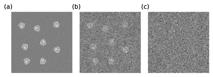
Figure 1. An example of the measurement $M$ defined in (1) with (a) SNR = $10^{2}$, (b) SNR = 1 and (c) SNR := $10^{-2}$, where $\text{SNR}=(\pi n^{2}\sigma^{2})^{-1}\sum_{x}F(x)^{2}$ .

Given the measurement $M$, the objective is to recover the function $f$. This problem is called multi-target detection (MTD) with rotations [8, 22]. Motivated by single-particle cryo-electron microscopy (cryo-EM), we focus on the low SNR regime, see Figure 1(c), where estimating the unknown translations and rotations is challenging [3, 7, 17]. We pose the following question.

Question.

Suppose that $M:\{1,\ldots,m\}^{2}\rightarrow\mathbb{R}$ is a measurement of the form described in (1) for fixed signal radius $n$ and density $\gamma$. If the variance of the noise $\sigma^{2}$ is fixed (but might be arbitrarily high), can the function $f$ be estimated from $M$ to any fixed level of accuracy when $m$ is sufficiently large?

In this paper, we develop a mathematical and computational framework for MTD with rotations, and show empirically that the answer to the above question is affirmative. In particular, we describe an autocorrelation analysis algorithm for recovering the function $f$ from the measurement $M$ and demonstrate its effectiveness and numerical stability. Additionally, in Section 3, we consider a simplified version of this statistical estimation problem in one dimension, where we are able to establish a theoretical foundation for this algorithm.

2. Motivation and related work

2.1. Motivation

Our interest in the MTD model arises from the structure determination problem for biological molecules. In the past decade, cryo-EM has emerged as a potent alternative to X-ray crystallography and nuclear magnetic resonance (NMR) spectroscopy to resolve the structures of proteins that either cannot be crystallized or are too complex for NMR. In cryo-EM, a solution that contains many copies of the target particle is rapidly cooled to form thin vitreous ice sheets whose thickness is comparable to the single molecule size. These sheets are then imaged with an electron microscope. The measurements in cryo-EM can be modeled as two-dimensional tomographic projections of identical biomolecules at unknown locations and orientations followed by some image distortion due to the imaging system. The projection images are embedded in a large, noisy image, called a micrograph. The crux of single-particle cryo-EM reconstruction is that, with sufficiently many micrographs, projection images of similar molecule orientations can be combined to improve the SNR and, in turn, reconstruct the high-resolution three-dimensional structure of the molecule.

The current computational pipeline for cryo-EM requires particle picking, the extraction of the biomolecule projection images from the micrographs [11, 13, 16, 34, 39, 38]. Then, the three-dimensional structure is built from the extracted images using a variety of algorithms [6, 14, 15, 27, 33, 36]. This approach is problematic for small particles where the SNR of micrographs is low, and detection becomes impossible [7, 17, 3]. As such, the difficulty of detection sets a lower bound on the usable molecule size in the current analysis workflow of cryo-EM data.

Interest in signal recovery beyond the detection limit has prompted the realization that the locations of the signal in the measurement are nuisance parameters; the emerging claim is that signal recovery can be achieved directly from the measurement [7]. Methodologies for direct image estimation have been inspired by Zvi Kam’s introduction of autocorrelation analysis to the structure reconstruction problem dealing with randomly oriented biomolecule projections [19]. The process involves accumulating the “spatial correlations”, or autocorrelations, of signal density in the measurements in order to average out the noise without estimating the rotations. These averages are then used for the reconstruction of the target image. Following Kam’s seminal paper on autocorrelations, several procedures based on correlations and moments have been proposed for cryo-EM and related modalities, e.g.,  [5, 9, 1, 24, 26, 31, 32, 35, 18].

Remark 2.1 (Relation of model of this paper to cryo-EM).

The model (1) considered in this paper involves a large noisy measurement $M$ that contains many instances of a 2D target image at arbitrary locations and random orientations. This model is a simplified version of cryo-EM data that, informally speaking, consists of a large noisy measurement that contains many tomographic projections of a 3D density at arbitrary locations and random orientations. While the 2D model we study is not directly applicable to cryo-EM data, it does represent a step towards understanding the application of invariant feature based approaches for cyro-EM by building upon past work on multi-target detection [8, 20, 21, 22, 40]. Moreover, the model considered in this paper corresponds to a degenerate case in cryo-EM in which the molecule has a preferred orientation. Random conical tilt [28] is a classical reconstruction method in cryo-EM that assumes a preferred orientation. The model considered in this paper has recently been extended to random conical tilt [23] which does have direct potential applications.

2.2. Related work

The problem addressed in this paper—with rotated and translated iterations of $f$ within $M$—extends previous works on the MTD model [8, 22]. In particular, we extend [25] by providing new theoretical understanding of a 1-dimensional model, and demonstrating empirically that reconstruction is possible from a measurement $M$ of the form (1). This is an important step toward the reconstruction of molecules in the undetectable domain. More generally, it attests to the possibility of direct image estimation from measurements so that limitations on particle picking do not necessarily translate to limitations on structure determination.

We mention that our results were recently extended, after this paper appeared online, to account for an arbitrary distribution of the target images [20]. In addition, an approximate expectation-maximization algorithm for the MTD model with rotations was developed in [22, 21], and a generalized method of moments framework was designed in [40].

3. One-Dimensional Problem

Before considering the two-dimensional problem (1), we introduce an analogous problem in one dimension. This simplified version will allow us to develop intuition for the autocorrelation framework we devise for the two-dimensional case.

3.1. Measurement

Let $F:\mathbb{Z}\rightarrow\mathbb{R}$ be a one-dimensional target signal supported on $\{-n,\ldots,n-1\}$, and $F_{\tau}:\mathbb{Z}\rightarrow\mathbb{R}$ be the result of cyclically rotating the support of $F$. That is, $F_{\tau}(x)=F((x+\tau)\bmod 2n)$ for $x\in\{-n,\ldots,n-1\}$, where we consider an integer modulo $2n$ to be an element of $\{-n,\ldots,n-1\}$, and $F_{\tau}(x)=0$ when $x\in\mathbb{Z}\setminus\{-n,\ldots,n-1\}$. Here, we will work with a one-dimensional analogue of the two-dimensional measurement defined in (1), where the measurement $M:\{1,\ldots,m\}\rightarrow\mathbb{R}$ is given by

(2) $$M(x)=\sum_{j=1}^{p}F_{\tau_{j}}(x-x_{j})+\varepsilon(x),$$

where $\tau_{1},\ldots,\tau_{p}\in\{-n,\ldots,n-1\}$ are uniformly random cyclic shifts; $x_{1},\ldots,x_{p}\in\{n+1,\ldots,m-n+1\}$ are arbitrary translations; and $\varepsilon$ is i.i.d. Gaussian noise on $\{1,\ldots,m\}$ with mean zero and variance $\sigma^{2}$. We plot an examples of the 1-dimensional measure $M$ with three different levels of noise in Figure 2.

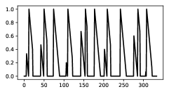
Figure 2. An example of the 1-dimensional measurement $M$ defined in (2) with $\text{SNR}=\infty$ (left), $\text{SNR}=10^{2}$ (middle), and $\text{SNR}=1$ (right), where $\text{SNR}:={(2}n{)}^{-1}\sum_{x}F(x)^{2}/\sigma^{2}$.

The circular shifts $\tau$ are the one-dimensional analogues of the two-dimensional rotations $\phi$ in (1). To extend the previous assumptions about the target separation and bounded density to this one-dimensional formulation, we assume that $|x_{j}-x_{k}|\geq 4n$ for all $k\not=j$ and that $np/m=\gamma>0$. In Theorem 3.2, we will additionally impose that the discrete Fourier transform (DFT) of $F$ is non-vanishing.

As above, our objective is to estimate the function $F$ from the measurement $M$ in the low SNR regime. In particular, we would like to show that $F$ can be reliably and accurately estimated from $M$ at any fixed level of noise, which might be arbitrarily high, as long as the size of the measurement $m$ is sufficiently large. The reliability and accuracy of this estimate will be quantified below. The approach is based on seeking features of $F$ that determine the function and are invariant to translations $F(x)\mapsto F(x+x^{\prime})$ and circular shifts of the support $F(x)\mapsto F_{\tau}(x)$. The construction of these invariant features is based on autocorrelation analysis.

3.2. Invariant features

Recall that $F:\mathbb{Z}\rightarrow\mathbb{R}$ is supported on $\{-n,\ldots,n-1\}$ and $F_{\tau}$ is a rotated version of $F$. We can define features of $F$ that are invariant to rotations and translations. The most direct example is the mean of the function

(3) $$T_{F}=\frac{1}{2n}\sum_{x=-n}^{n-1}F(x).$$

Motivated by autocorrelation analysis, the mean above can also be interpreted as the first-order autocorrelation. The rotationally-averaged second-order autocorrelation $U_{F}:\{-2n,\ldots,2n-1\}\to\mathbb{R}$ is defined by

$$U_{F}(x_{1})=\frac{1}{2n}\sum_{\tau=-n}^{n-1}\frac{1}{2n}\sum_{x=-n}^{n-1}F_{\tau}(x)F_{\tau}(x+x_{1}).$$

Considering the sum geometrically (or by a change of variables) we observe that $U_{F}(x_{1})$ is only a function of the magnitude $|x_{1}|$, and so, cannot contain sufficient information to recover $F$. Thus, the critical invariant is the rotationally-averaged third-order autocorrelation $V_{F}:\{-2n,\ldots,2n-1\}^{2}\rightarrow\mathbb{R}$, which is defined by

(4) $$V_{F}(x_{1},x_{2})=\frac{1}{2n}\sum_{\tau=-n}^{n-1}\frac{1}{2n}\sum_{x=-n}^{n-1}F_{\tau}(x)F_{\tau}(x+x_{1})F_{\tau}(x+x_{2}).$$

By construction, both $U_{F}(x_{1})$ and $V_{F}(x_{1},x_{2})$ are invariant under translations $F(x)$ $\mapsto F(x-x^{\prime})$ and rotations $F(x)\mapsto F_{\tau^{\prime}}(x)$. That is, $U_{F}=U_{G}$ and $V_{F}=V_{G}$ when $G(x)=F_{\tau^{\prime}}(x+x^{\prime})$ for any $\tau^{\prime}\in\{-n,\ldots,n-1\}$ and $x^{\prime}\in\mathbb{Z}$.

3.3. Estimation from measurement

The function $V_{F}:\{-2n,\ldots,2n-1\}^{2}\rightarrow\mathbb{R}$ can be estimated from a measurement $M:\{1,\ldots,m\}\rightarrow\mathbb{R}$ of the form described in §3.1. For simplicity, let us extend the separation condition so that it also holds periodically in the sense that $|x_{k_{1}}-x_{k_{2}}-m|>4n$. We define the third-order autocorrelation of the measurement $A_{M}:\{-2n\ldots,2n-1\}^{2}\rightarrow\mathbb{R}$ by

(5) $$A_{M}(x_{1},x_{2})=\\ \frac{1}{m}\sum_{x=1}^{m}M(x)M(x+x_{1}\bmod m)M(x+x_{2}\bmod m),$$

where an integer modulo $m$ is taken as an element of $\{1,\ldots,m\}$.

The following lemma shows that $V_{F}$ can be estimated from $A_{M}$ (namely, from the data) if $m$ is much larger than $\sigma^{6}$. Information theoretic results that were derived for a closely related model called multi-reference alignment indicate that this is the optimal estimation rate in the low SNR regime where $m,\sigma\to\infty$ while $\gamma$ and $n$ are fixed [2, 5, 26].

Lemma 3.1.

Suppose that $|F|<F_{max}$ everywhere for some constant $F_{max}>0$. Under the one-dimensional model (2), we have:

$$\mathbb{E}(A_{M}(x_{1},x_{2}))=\frac{\gamma}{n}V_{F}(x_{1},x_{2})+2\gamma T_{F}\sigma^{2}(\delta_{0}(x_{1}-x_{2})+\delta_{0}(x_{1})+\delta_{0}(x_{2})),$$

and

$$\operatorname{Var}\left(A_{M}(x_{1},x_{2})\right)=\mathcal{O}\left(\frac{n}{m}\left(\gamma F_{max}^{6}+\sigma^{6}\right)\right),$$

where the expectation and variance are taken with respect to the random cyclic shifts and the Gaussian noise, and $\delta_{0}(x)=1$ when $x=0$ and $\delta_{0}(x)=0$ otherwise.

Proof.

See Appendix A. ∎

The retrieval of $F$ from $V_{F}$, combined with Lemma 3.1, would result in the extraction of $F$ from the measurement $M$ up to a rotation, given a sufficiently large measurement.

3.4. Recovery from invariant features

The DFT of the function $F:\mathbb{Z}\rightarrow\mathbb{R}$ considered as a function on its support $\{-n,\ldots,n-1\}$ is defined by

(6) $$a_{k}:=\sum_{x=-n}^{n-1}F(x)e^{-2\pi ikx/(2n)},\quad k\in\{-n,\ldots,n-1\}.$$

We now show that $V_{F}$ determines $F$ via a closed form when its DFT is non-vanishing. We remark that such a non-vanishing condition is standard for problems related to autocorrelation inversion, see for example [9, 26].

Theorem 3.2.

Suppose that the DFT of $F$ expressed in (6) is non-vanishing. Then, $\tilde{F}$ can be determined from $V_{F}$ via a closed form expression (resulting from inverting a linear system only depending on $n$) such that $\tilde{F}=F_{\tau}$ for some $\tau\in\{-n,\ldots,n-1\}$. That is, $F$ can be recovered up to a circular shift.

Proof.

Let $A_{F}:\{-2n,\ldots,2n-1\}^{2}\rightarrow\mathbb{R}$ designate the third-order autocorrelation

(7) $$A_{F}(x_{1},x_{2})=\\ \frac{1}{2n}\sum_{x=-2n}^{2n-1}F(x)F((x+x_{1})\bmod 4n)F((x+x_{2})\bmod 4n),$$

where an integer modulo $4n$ is taken to be element of $\{-2n,\ldots,2n-1\}$. Observe that we have

$$V_{F}(x_{1},x_{2})=\frac{1}{2n}\sum_{\tau=-n}^{n-1}A_{F_{\tau}}(x_{1},x_{2}).$$

Indeed, since $F$ is supported on $\{-n,\ldots,n-1\}$, taking it as a periodic function in (7) does not change the result. Let $b_{m}$ denote the Fourier coefficients of $F$ considered as a periodic function on $\{-2n,\ldots,2n-1\}$; that is,

$$b_{m}:=\sum_{x=-n}^{n-1}F(x)e^{-2\pi imx/(4n)}.$$

By Fourier inversion on the interval $\{-2n,\ldots,2n-1\}$, we have

(8) $$F(x)=\frac{1}{4n}\sum_{m=-2n}^{2n-1}b_{m}e^{2\pi imx/(4n)}.$$

Substituting the representation of $F(x)$ in terms of the coefficients $b_{m}$ into $A_{F}$ and summing over $x$ yields

$$A_{F}(x_{1},x_{2})=\frac{1}{2n}\frac{1}{(4n)^{3}}\cdot\\ \sum_{m_{1},m_{2}=-2n}^{2n-1}b_{m_{1}}b_{m_{2}}b_{-m_{1}-m_{2}}e^{2\pi i(m_{1}x_{1}+m_{2}x_{2})/(4n)}.$$

Next, by taking the two-dimensional DFT of $A_{F}(x_{1},x_{2})$ on $\{-2n,\ldots,2n-1\}^{2}$, we can recover $b_{m_{1}}b_{m_{2}}b_{-m_{1}-m_{2}}$ for $m_{1},m_{2}\in\{-2n,\ldots,2n-1\}$:

$$b_{m}=\sum_{j=-n}^{n-1}\left(\frac{1}{2n}\sum_{k=-n}^{n-1}a_{k}e^{2\pi ikj/(2n)}\right)e^{-2\pi imj/(4n)}\\ =\sum_{k=-n}^{n-1}\gamma_{m,k}a_{k},$$

where

$$\gamma_{m,k}:=\frac{1}{2n}\sum_{j=-n}^{n-1}e^{2\pi ikj/(2n)}e^{-2\pi imj/(4n)}.$$

Observe that if $m=2k^{\prime}$ we have $\gamma_{m,k^{\prime}}=1$ and $\gamma_{m,k}=0$ if $k\not=k^{\prime}$. It follows that

$$b_{2k_{1}}b_{2k_{2}}b_{-2k_{1}-2k_{2}}=a_{k_{1}}a_{k_{2}}a_{-k_{1}-k_{2}}$$

for $k_{1},k_{2}\in\{-n,\ldots,n-1\}$. The quantity $a_{k_{1}}a_{k_{2}}a_{-k_{1}-k_{2}}$, called the bispectrum of the function $F$, is invariant under cyclic shifts of the underlying function $F$ and determines $F$ uniquely, up to a global cyclic shift  [9, 30, 37]. More precisely, by taking the logarithm of the bispectrum we arrive at a linear system of equations which is full rank after the cyclic shift ambiguity is removed, see [9, §IV.C]. Therefore, for each $n$, there is a fixed linear transform that determines the Fourier coefficients of $F$, up to a phase ambiguity. Since the reduction of $V_{F}$ to the bispectrum can also be accomplished by a linear transform, for any fixed $n$ composing these linear transformations together with Fourier inversion gives a closed form expression for determining $F$ up to cyclic shift from $V_{F}$. Thus, given $V_{F}$, we can determine $\tilde{F}=F_{\tau}$ for some $\tau\in\{-n,\ldots,n-1\}$, as desired. ∎

Example 3.3.

To illustrate the approximation result of Lemma 3.1 and Theorem 3.2, we present a basic numerical example. We use the signal from Figure 2 with $\text{SNR}=10^{2}$. Next, we form a measurement of the form (2) with various numbers of samples $p$ of the given function. We use the identities described in the proof of Theorem 3.2 to approximate the bispectrum $a_{k_{1}}a_{k_{2}}a_{-k_{1}-k_{2}}$ for $k_{1},k_{2}\in\{-n,\ldots,n-1\}$ of the given signal $F$. We plot the relative error of the bispectrum extracted from the measurement compared to the ground truth, see Figure 3. The error decreases as $1/\sqrt{p}$, as expected by the law of large numbers. The function can be recovered from the bispectrum using a variety of standard methods, see [9].

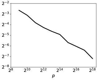
Figure 3. Relative error of bispectrum derived from measurement $M$ using various number of samples $p$ averaged over 10 trials. The error decreases as $1/\sqrt{p}$, as expected by the law of large numbers.

Remark 3.4 (Discretization model).

In the above model, we consider a function $F$ defined on a gird that is transformed by on grid translations. One potential extension of this model is to consider off grid translations by assuming that $F$ represents samples from an underlying function $f$ defined on the real-line; more precisely, the model (2) could be extended by introducing a shift parameter $\delta\in[0,1/n)$ and defining

$$F^{\delta}(x)=f(x/n+\delta),$$

for a discretization parameter $n\in\mathbb{Z}_{>0}$ and an underlying function $f:\mathbb{R}\rightarrow\mathbb{R}$ that is supported on $[-1,1]$. With this notation, the measurement model (2) could be extended by defining $M:\{1,\ldots,m\}\rightarrow\mathbb{R}$ by

$$M(x)=\sum_{j=1}^{p}F_{\tau_{j}}^{\delta_{j}}(x-x_{j})+\varepsilon(x),$$

where $\tau_{j}\in\{-n,\ldots,n-1\}$ is a random cyclic rotation, $x_{j}\in\{n+1,\ldots,m-n+1\}$ are arbitrary translations, $\varepsilon$ is i.i.d. Gaussian noise on $\{1,\ldots,m\}$, and $\delta_{j}\in[0,1/n]$ is a random shift. Under this model, the third-order autocorrelation $A_{M}(x_{1},x_{2})$ defined in (5) would satisfy an analogous version of Lemma 3.1, where the features $T_{F}$ and $V_{F}$ are replaced by quantities defined with appropriate integrals instead of sums. Studying this extended model would require quantifying an additional source of error when trying to determine $f$ from its third-order autocorrelation; in particular, it would be necessary to make assumptions justifying why the Fourier inversion formula (8) approximately holds (for example, one could assume that $f$ is Lipchitz continuous, or assume that $f$ and its derivatives are Lipchitz continuous up to order $k$ such that classical approximation theory results could be employed).

In this paper, we focus on translations on the discretization grid (for both the 1D and 2D models we consider) to avoid dealing with this additional source of approximation error. Our goal in considering on grid translations is to study the simplest possible model that still captures the essence of the signal processing problem of interest: MTD in a setting where there are two different types of random linear actions. Extending the results of this paper to handle arbitrary shifts would be a necessary extension if the presented approaches are adapted for an application problem involving real data.

4. Two-dimensional problem

After having established the theoretical foundation for the one-dimensional problem above, we aim to extend the recovery of the underlying function $f$ to two dimensions. In order to make this estimation tractable, it is necessary to make regularity assumptions on the function $f$; we build the foundation for these assumptions below.

4.1. Invariant features in the continuous setting

As in §3.2, we define the continuous two-dimensional analogues for the features of $f$ that are invariant under translations and rotations. As before, the first invariant is the mean of the function

$$q_{f}:=\int_{\mathbb{R}^{2}}f(x)dx.$$

Letting $f_{\phi}$ be the rotation of $f$ by angle $\phi$ about the origin, we define rotationally-averaged second-order autocorrelation $r_{f}:\mathbb{R}^{2}\rightarrow\mathbb{R}$ by

$$r_{f}(x_{1}):=\frac{1}{2\pi}\int_{0}^{2\pi}\int_{\mathbb{R}^{2}}f_{\phi}(x)f_{\phi}(x+x_{1})dxd\phi.$$

Finally, to gain enough information for the recovery of $f$, the rotationally-averaged third-order autocorrelation $s_{f}:\mathbb{R}^{2}\times\mathbb{R}^{2}\rightarrow\mathbb{R}$ is

$$s_{f}(x_{1},x_{2}):=\frac{1}{2\pi}\int_{0}^{2\pi}\int_{\mathbb{R}^{2}}f_{\phi}(x)f_{\phi}(x+x_{1})f_{\phi}(x+x_{2})dxd\phi.$$

In this case, observe that $s_{f}$ is a function of $|x_{1}|,|x_{2}|$ and the angle $\theta(x_{1},x_{2})$ between $x_{1}$ and $x_{2}$. Geometrically, as a function of three variables, $s_{f}$ potentially contains enough information to recover $f$.

4.2. Invariant features in the discrete setting

As in the one-dimensional case, we will focus on the recovery of some discretization of $f$ from some discretization of $s_{f}$ under similar assumptions to those in Theorem 3.2. Restricting our attention to this problem is consistent with the fact that actual measurements are discretized over a pixel grid. Conveniently, this also considerably simplifies the presentation of the method.

We define the discretization $F_{\phi}:\mathbb{Z}^{2}\rightarrow\mathbb{R}$ of $f_{\phi}$ by

$$F_{\phi}(x)=f_{\phi}(x/n),\quad\text{for}\quad x\in\mathbb{Z}^{2},$$

where $n$ is a fixed integer that determines the sampling resolution. We define the discrete rotationally-averaged third-order autocorrelation $S_{f}:\mathbb{Z}^{2}\times\mathbb{Z}^{2}\rightarrow\mathbb{R}$ by

(9) $$S_{F}(x_{1},x_{2}):=\\ \frac{1}{2\pi}\int_{0}^{2\pi}\frac{1}{4n^{2}}\sum_{x\in\mathbb{Z}^{2}}F_{\phi}(x)F_{\phi}(x+x_{1})F_{\phi}(x+x_{2})d\phi.$$

Since $f_{\phi}$ is supported on the open unit disc $\{x\in\mathbb{R}^{2}:|x|<1\}$, it follows that $F_{\phi}$ is supported on $\{x\in\mathbb{Z}^{2}:|x|<n\}$, and $S_{F}(x_{1},x_{2})$ is supported on

$$\mathcal{X}:=\{-2n,\ldots,2n-1\}^{2}\subset\mathbb{Z}^{2},$$

which contains $(2n)^{2}$ points.

4.3. Estimation from measurement

Suppose that $M:\{1,\ldots,m\}^{2}\rightarrow\mathbb{R}$, a measurement of the form in (1), is given. We define the third-order autocorrelation of $M$ as $A_{M}:\mathbb{Z}^{2}\times\mathbb{Z}^{2}\rightarrow\mathbb{R}$ by

$$A_{M}({x}_{1},{x}_{2}):=\frac{1}{m^{2}}\sum_{{x}\in\mathbb{Z}^{2}}M({x})M({x}+{x}_{1})M({x}+{x}_{2}).$$

Recall that the measurement $M:\{1,\ldots,m\}^{2}\rightarrow\mathbb{R}$ is defined by

$$M({x})=\sum_{j=1}^{p}F_{\phi_{j}}(x-x_{j})+\varepsilon({x}),$$

where $\phi_{j}$ are random angles, $x_{j}$ are translations, and $\varepsilon$ is noise (see §1). As before, we assume that images in $M$ are separated by at least one image diameter according to

$$|{x}_{j_{1}}-{x}_{j_{2}}|\geq 4n,\quad\text{for}\quad j_{1}\not=j_{2},$$

and that the density of the target images in the measurement is $pn^{2}/m^{2}=\gamma$ for a fixed constant $\gamma>0$. Under these assumptions, it is straightforward to show that for any fixed level of noise $\sigma^{2}$, fixed signal radius $n$ and fixed $\gamma$,

(10) $$A_{M}({x}_{1},{x}_{2})\rightarrow\frac{\gamma}{2\pi}S_{F}({x}_{1},{x}_{2})+\\ \frac{\gamma}{2\pi}\sigma^{2}\mu_{F}\big{(}\delta({x_{1}})+\delta({x_{2}})+\delta({x_{1}}-{x_{2}})\big{)},$$

as $m\rightarrow\infty$ (see for example [7]), where $\mu_{F}$ is the discrete mean of $F$ defined by

$$\mu_{F}=\frac{1}{4n^{2}}\sum_{x\in\mathbb{Z}^{2}}F_{\phi}(x).$$

As such, (10) relates the third-order autocorrelation of the measurement $A_{M}$ to the invariant features $S_{F}$ and $\mu_{F}$. In practice, $\sigma^{2}$ and $\gamma\mu_{F}$ can be estimated from $M$: $\sigma^{2}$ can be estimated by the variance of the pixel values of $M$ in the low SNR regime, while $\gamma\mu_{F}$ can be estimated by the empirical mean of $M$. As a result, $S_{F}$, a feature of the image, can be estimated from $A_{M}$, a feature of the measurement, up to a constant factor.

4.4. Band-limited functions on the unit disc

The Dirichlet Laplacian eigenfunctions on the unit disc $D=\{(x,y)\in\mathbb{R}:x^{2}+y^{2}\leq 1\}$ are solutions to the eigenvalue problem

$$\left\{\begin{array}[]{cc}-\Delta\psi=\lambda\psi&\text{in }D\\ \psi=0&\text{on }\partial D,\end{array}\right.$$

where $-\Delta=-(\partial_{xx}+\partial_{yy})$ is the Laplacian, and $\partial D$ is the boundary of the unit disc. In polar coordinates $(r,\theta)$, these eigenfunctions are of the form

(11) $$\psi_{\nu,q}(r,\theta)=J_{\nu}\left(\lambda_{\nu,q}r\right)e^{i\nu\theta},$$

where $\nu\in\mathbb{Z}_{\geq 0}$, $J_{\nu}$ is the $\nu$-th order Bessel function of the first kind, and $\lambda_{n,q}>0$ is the $q$-th positive root of $J_{\nu}$. Recall that $J_{\nu}$ is a solution to the differential equation

$$y^{\prime\prime}(r)+\frac{1}{r}y^{\prime}(r)+\left(1-\frac{\nu^{2}}{r^{2}}\right)y(r)=0.$$

Therefore, by writing the Laplacian $-\Delta$ in polar coordinates, we have

$$-\Delta\psi_{\nu,q}(r,\theta)=-\left(\partial_{rr}+\frac{1}{r}\partial_{r}+\frac{1}{r^{2}}\partial_{\theta\theta}\right)\psi_{\nu,q}(r,\theta)=\lambda_{\nu,q}^{2}\psi_{\nu,q}(r,\theta),$$

and, as such, $\lambda_{\nu,q}^{2}$ is the eigenvalue corresponding to the eigenfunction $\psi_{\nu,q}$. Therefore, the projection operator

$$P_{\lambda}f=\sum_{(\nu,q):\lambda_{\nu,q}\leq\lambda}\frac{\langle f,\psi_{\nu,q}\rangle}{\|\psi_{\nu,q}\|_{2}^{2}}\psi_{\nu,q}$$

can be viewed as a low-pass filter for functions on the unit disc; we call functions that are invariant under this projection operator band-limited functions.

4.5. Steerable bases

Recall that $f:\mathbb{R}^{2}\rightarrow\mathbb{R}$ is supported on the unit disc. Using the notation from §4.4, the assumption that $f$ is band-limited on its support can be written as

(12) $$f(r,\theta)=\sum_{(\nu,q):\lambda_{\nu,q}\leq\lambda}\alpha_{\nu,q}\psi_{\nu,q}(r,\theta),\quad\text{for }r\leq 1,$$

where $\lambda>0$ is the band-limit frequency, and $\alpha_{\nu,q}$ are expansion coefficients. For each $\nu$, we define

$$g_{\nu}(r,\theta)=\sum_{q:\lambda_{\nu,q}\leq\lambda}\alpha_{\nu,q}\psi_{\nu,q}(r,\theta)=\\ \left(\sum_{q:\lambda_{\nu,q}\leq\lambda}\alpha_{\nu,q}J_{\nu}\left(\lambda_{\nu,q}r\right)\right)e^{i\nu\theta},$$

so that we can write $f$ by

(13) $$f(r,\theta)=\sum_{\nu=-N}^{N}g_{\nu}(r,\theta),$$

where $N:=\max\{\nu:\lambda_{\nu,1}\leq\lambda\}$.

The advantage of expressing a function in terms of Dirichlet Laplacian eigenfunctions is that the basis is steerable—the effect of rotations on expansion coefficients of the images are expressed as phase modulation. Specifically, a steerable basis diagonalizes the rotation operator so that the rotation $f_{\phi}(r,\theta):=f(r,\theta+\phi)$ of $f$ about the origin by angle $\phi$ can be computed by multiplying each term in the sum in (13) by $e^{i\nu\phi}$:

(14) $$f_{\phi}(r,\theta)=\sum_{\nu=-N}^{N}g_{\nu}(r,\theta)e^{i\nu\phi}.$$

From this point forward, we will switch between considering functions in polar coordinates $f(r,\theta)$ or Cartesian coordinates $f({x})$, where ${x}=(r\cos\theta,r\sin\theta)$, depending on which is more convenient.

4.6. Using the band-limited assumption

We now take advantage of the assumption that $f$ is band-limited on the unit disc. Let $\Psi_{\nu,q}:\mathcal{X}\rightarrow\mathbb{C}$ be the discretization of the Dirichlet Laplacian eigenfunctions

$$\Psi_{\nu,q}(x)=\psi_{\nu,q}(x/n),$$

where $\psi_{\nu,q}$ is supported on the unit disc, as in §4.4. With this notation,

$$F_{\phi}(x)=\sum_{(\nu,q):\lambda_{\nu,q}\leq\lambda}\alpha_{\nu,q}\Psi_{\nu,q}(x)e^{i\nu\phi}.$$

By considering $F_{\phi}$ and $S_{F}$ as functions on $\mathcal{X}$, we can express their DFT $\hat{F}_{\phi}:\mathcal{X}\rightarrow\mathbb{C}$ by

$$\hat{F}_{\phi}(k)=\sum_{x\in\mathcal{X}}F_{\phi}(x)e^{-2\pi ix\cdot k/(4n)}.$$

Finally, we let $\hat{\Psi}_{\nu,q}:\mathcal{X}\rightarrow\mathbb{C}$ be the DFT of $\Psi_{\nu,q}:\mathcal{X}\rightarrow\mathbb{C}$

$$\hat{\Psi}_{\nu,q}(k)=\sum_{x\in\mathcal{X}}\Psi_{\nu,q}(x)e^{-2\pi ix\cdot k/(4n)}.$$

Then, by the linearity of the DFT it follows from the previous section that

$$\hat{F}_{\phi}(k)=\sum_{(\nu,q)\in\mathcal{V}}\alpha_{\nu,q}\hat{\Psi}_{\nu,q}(k)e^{i\nu\phi},$$

where $\mathcal{V}=\{(\nu,q):\lambda_{\nu,q}\leq\lambda\}$.

4.7. Discrete Fourier transform of invariant features

The Fourier transform defined in the previous section can now be related to the Fourier transform of $S_{F}$. We define $\hat{S}_{F}:\mathcal{X}\times\mathcal{X}\rightarrow\mathbb{C}$ by

(15) $$\hat{S}_{F}(k_{1},k_{2}):=\sum_{x_{1}\in\mathcal{X}}\sum_{x_{2}\in\mathcal{X}}S_{F}(x_{1},x_{2})e^{-2\pi i(k_{1}\cdot x_{1}+k_{2}\cdot x_{2})/4n},$$

where addition is considered modulo $4n$ with $-2n,\ldots,2n-1$ as the representatives of the different equivalence classes. Substituting (9) into (15) and simplifying gives

$$\hat{S}_{F}(k_{1},k_{2})=\int_{0}^{2\pi}\hat{F}_{\phi}(k_{1})\hat{F}_{\phi}(k_{2})\hat{F}_{\phi}(-k_{1}-k_{2})d\phi.$$

This integral over $\phi$ can be replaced by a summation over the rotations at the Nyquist rate so that the expression becomes:

(16) $$\hat{S}_{F}(k_{1},k_{2})=\sum_{j=0}^{6N-1}\hat{F}_{\phi_{j}}(k_{1})\hat{F}_{\phi_{j}}(k_{2})\hat{F}_{\phi_{j}}(-k_{1}-k_{2}),$$

where $\phi_{j}:=2\pi j/(6N)$. If $N:=\max\{\nu:\lambda_{\nu,1}\leq\lambda\}$, then the products $F_{\phi}(x)F_{\phi}(x+x_{1})F_{\phi}(x+x_{2})$ that appear in (16) are band-limited by $N$ with respect to $\phi$. Also, note that the summand on the right hand side of (16) is the DFT of the third autocorrelation of a function and is called the bispectrum [9, 30, 37]. We encountered the one-dimensional analogue of the bispectrum at end of the proof to Proposition 3.2.

4.8. Vector notation

Recall the enumeration $\mathcal{V}$ from §4.6, which consists of $(\nu_{1},q_{1}),\ldots,(\nu_{d},q_{d})$ such that

$$\hat{F}_{\phi}(k)=\sum_{j=1}^{d}\alpha_{\nu_{j},q_{j}}\hat{\Psi}_{\nu_{j},q_{j}}(k)e^{i\nu_{j}\phi},$$

for $k\in\mathcal{X}$. For a fixed angle $\phi$ and $k\in\mathcal{X}$, we define the vector $u(\phi,k)\in\mathbb{R}^{d}$ by

$$u_{j}(\phi,k)=\hat{\Psi}_{\nu_{j},q_{j}}(k)e^{i\nu_{j}\phi}.$$

Thus, each vector $v\in\mathbb{R}^{d}$ defines the DFT of a band-limited function by

$$\hat{F}_{v,\phi}(k)=\sum_{j=1}^{n}v_{j}u_{j}(\phi,k)=v^{\top}u(\phi,k),$$

where $v^{\top}$ is the transpose of $v$. The following lemma is immediate from (16) and the product rule.

Lemma 4.1.

We have

$$\hat{S}_{F_{v}}({k}_{1},{k}_{2})=\\ \sum_{j=0}^{6N-1}v^{\top}u(\phi_{j},k_{1})v^{\top}u(\phi_{j},k_{2})v^{\top}u(\phi_{j},-{k}_{1}-{k}_{2})$$

where $\phi_{j}:=2\pi j/(6N)$. Moreover, the $d$-dimensional gradient $\nabla_{v}\hat{S}_{F_{v}}$ satisfies

$$\nabla_{v}\hat{S}_{F_{v}}(k_{1},k_{2})=\sum_{j=0}^{6N-1}\Big{(}v^{\top}u(\phi_{j},k_{1})v^{\top}u(\phi_{j},k_{2})u(\phi_{j},-k_{1}-k_{2})\\ +v^{\top}u(\phi_{j},k_{1})v^{\top}u(\phi_{j},-k_{1}-k_{2})u(\phi_{j},k_{2})\\ +v^{\top}u(\phi_{j},k_{2})v^{\top}u(\phi_{j},-k_{1}-k_{2})u(\phi_{j},k_{1})\Big{)}.$$

In the next section, we describe how to estimate $S_{F}$ from a measurement $M$ and form an optimization problem to recover the target image $F$ from the measurement $M$.

4.9. Computational complexity

For some intuition regarding the computational complexity of computing $\hat{S}_{F_{v}}$ and $\nabla_{v}S_{F_{v}}$, recall that $\mathcal{X}=\{-2n,\ldots,2n-1\}^{2}$ so that, crudely, the image $F$ has $\sim n^{2}$ pixels. In the following, we make the assumption that the number of eigenfunctions used to expand the function $F$ should not exceed the number of pixels in the image. Notationally, $|\mathcal{V}|=\mathcal{O}(n^{2})$.

Proposition 4.2.

We can compute $\hat{S}_{F_{v}}(k_{1},k_{2})$ and $\nabla_{v}\hat{S}_{F_{v}}(k_{1},k_{2})$ for all $(k_{1},k_{2})\in\mathcal{X}^{2}$ in $\mathcal{O}(n^{5})$ operations.

Proof.

First, we compute $v^{\top}u(\phi_{j},k)$ for $j=0,\ldots,6N-1$ and $k\in\mathcal{X}$. Each inner product resolves to $\mathcal{O}(n^{2})$ operations for $\mathcal{O}(Nn^{2})$ total evaluations. Eigenvalue asymptotics show that $N$ is of the order of $\sqrt{|\mathcal{V}|}=\mathcal{O}(n)$ so this computation involves $\mathcal{O}(n^{5})$ operations.

After this pre-computation, it is straightforward to calculate $\hat{S}_{F_{v}}(k_{1},k_{2})$ for all $(k_{1},k_{2})\in\mathcal{X}^{2}$ in $\mathcal{O}(n^{5})$ operations. For $\nabla_{v}\hat{S}_{F_{v}}(k_{1},k_{2})$, the key observation is that the gradient is a linear combination of $\mathcal{O}(n^{3})$ vectors of length $\mathcal{O}(n^{2})$. First, we compute the coefficients in $\mathcal{O}(n^{5})$ operations and then sum the vectors in $\mathcal{O}(n^{5})$ operations.

∎

5. Algorithms and Numerical Results

5.1. Optimization problem

We now delineate an optimization problem for the estimation of $F$ from $S_{F}$. Recall that each vector $v\in\mathbb{R}^{d}$ defines the Fourier transform of a band-limited function on the disc by

$$\hat{F}_{v,\phi}(k)=v^{\top}u(\phi,k),$$

as in §4.8. We define the least squares cost function $g:\mathbb{R}^{d}\rightarrow\mathbb{R}$ by

$$g(v)=\frac{1}{2}\sum_{(k_{1},k_{2})\in\mathcal{X}^{2}}\left(\hat{S}_{F_{v}}(k_{1},k_{2})-\hat{S}_{F}(k_{1},k_{2})\right)^{2}.$$

Using the chain rule, the gradient of $\nabla g$ is

$$\nabla g(v)=\\ \sum_{(k_{1},k_{2})\in\mathcal{X}^{2}}\left(\hat{S}_{F_{v}}(k_{1},k_{2})-\hat{S}_{F}(k_{1},k_{2})\right)\nabla_{v}\hat{S}_{F_{v}}(k_{1},k_{2}),$$

where $\hat{S}_{F_{v}}$ and $\nabla_{v}\hat{S}_{F_{v}}$ can be computed via the formulas in Lemma 4.1.

5.2. Recovery from invariant features

Given a cost function and a gradient, there are a variety of optimization methods that can be used. For simplicity, we use the Broyden-Fletcher-Goldfarb-Shanno (BFGS) algorithm, which is a popular gradient-based optimization method.

First, we consider the problem of recovering $F$ from $S_{F}$ in the absence of noise. We generate a band-limited image $F$ by projecting a $65\times 65$ image of a tiger onto the span of the first $600$ Dirichlet Laplacian eigenfunctions as in Figure 4.

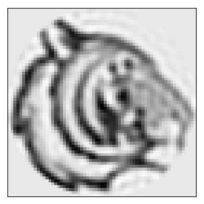
Figure 4. The projection of a $65\times 65$ image of a tiger onto the span of the first $600$ Dirichlet Laplacian eigenfunctions on a disc.

Using the BFGS optimization algorithm, the image in Figure 4 can be recovered with reconstruction error $\text{error}_{\text{recon}}=5\times 10^{-12}$. This optimization takes $6.5\times 10^{4}$ seconds parallelized over 100 CPUs in total.

Remark 5.1 (Computational limitations of implementation).

We use 600 eigenfunctions for this example due to computational limitations. The method was implemented as a CPU code, but is highly amiable to parallelization. Implementing the method described in this paper to support the use of GPUs would greatly increase the number of images and eigenfunctions that could be considered; however, since our goal is to present a proof-of-concept of the method, we choose not to pursue this optimization of the code for our numerical results; however, creating a GPU version of the method is an interesting potential extension of this work.

5.3. Using symmetry to average noise

Recall that $S_{F}(x_{1},x_{2})$ is a discrete version of $s_{f}:\mathbb{R}^{2}\times\mathbb{R}^{2}\rightarrow\mathbb{R}$ by

$$s_{f}(x_{1},x_{2}):=\frac{1}{2\pi}\int_{0}^{2\pi}\int_{\mathbb{R}^{2}}f_{\phi}(x)f_{\phi}(x+x_{1})f_{\phi}(x+x_{2})dxd\phi,$$

which only depends on the three parameters: the magnitudes $|{x}_{1}|$, $|{x}_{2}|$ and the angle $\theta({x}_{1},{x}_{2})$ between $x_{1}$ and $x_{2}$. Moreover, the Fourier transform $\hat{s}_{f}$ of $s_{f}$ will have these same symmetries. So, it follows that $\hat{S}_{F}$, which is a discrete version of $\hat{s}_{f}$, will also approximately exhibit these symmetries.

However, since $S_{F}$ is sampled on a grid, the symmetry will not be exact. In order to still take advantage of the expected symmetry when $S_{F}(x_{1},x_{2})$ is estimated from a noisy measurement $M$, we introduce a “binning” function. Let $b:\mathcal{X}\times\mathcal{X}\rightarrow\mathbb{Z}^{3}$ be defined by

$$b({k}_{1},{k}_{2})=\left(\left\lfloor b_{1}|{k}_{1}|\right\rfloor,\left\lfloor b_{1}|{k}_{2}|\right\rfloor,\left\lfloor b_{2}\theta({k}_{1},{k}_{2})\right\rfloor\right),$$

for fixed parameters $b_{1},b_{2}\in\mathbb{R}$ and $\mathcal{T}\subset\mathbb{Z}^{3}$ be the range of $b$. The corresponding cost function $g_{b}:\mathbb{R}^{d}\rightarrow\mathbb{R}$ is then

$$g_{b}(v)=\frac{1}{2}\sum_{T\in\mathcal{T}}\left(\sum_{(k_{1},k_{2})\in I_{T}}\left(\hat{S}_{F_{v}}(k_{1},k_{2})-\hat{S}_{F}(k_{1},k_{2})\right)\right)^{2},$$

such that

$$\nabla g_{b}(v)=\sum_{T\in\mathcal{T}}\left(\sum_{(k_{1},k_{2})\in I_{T}}\hat{S}_{F_{v}}(k_{1},k_{2})-\hat{S}_{F}(k_{1},k_{2})\right)\cdot\sum_{(k_{1},k_{2})\in I_{T}}\nabla\hat{S}_{F_{v}}(k_{1},k_{2}),$$

where $I_{T}=\{(k_{1},k_{2})\in\mathcal{X}^{2}:b(k_{1},k_{2})=T\}$ is the pre-image of $T$ under $b$. This is the same as the cost function $g(v)$ above except that the elements are now summed within the same symmetric bin $I_{T}$. For the numerical results reconstructing $F$ from a noisy measure, we report errors with binning.

Remark 5.2 (Estimating noise level).

In the following numerical example, we assume that the noise level is known. However, for applications it would be necessary to estimate the noise level. In standard cryo-EM experiments, estimating the statistics of the noise is part of the standard computational pipeline [6]. If the noise dominates the signal—which is the regime of interest of this paper—then it may be easy to get a good initial guess of the noise level; see for example [13]. Afterwards, the noise could be estimated iteratively, or the algorithm could be run at various noise levels.

Remark 5.3 (Uniform in-plane rotation).

In cryo-EM, the in-plane rotations are uniformly distributed since the specific rotation of the micrograph is arbitrarily chosen by the practitioner and there is no physics reason for bio-molecules to prefer a given orientation. In contrast, the viewing directions distribution is typically non-uniform due to several physic reasons, such as specimen adherence to the air-water interface [4].

5.4. Recovery from noisy micrographs

Returning to the original problem presented in §1, we recall the problem of recovering a band-limited image $f$ from a measurement $M$ as the size $m$ of the measurement tends to infinity. To approximate the behavior practically, for both computational purposes and reflecting the applications to cryo-EM, we fix $m=1000$ and call a $1000\times 1000$ measurement $M$ a micrograph. The numerical experiments follow the model described in this paper: we define each $1000\times 1000$ micrograph by (1). We compute the third order autocorrelation $A_{M}$ as defined by §4.3; we assume that $\gamma$ and $\sigma$ are known for simplicity.

We report numerical results in terms of the number of independent micrographs that are used. In particular, we report both the relative error in the invariant $S_{F}$ and the recovery of the image $F$. The error for $S_{F}$ is summed over the bins while the relative error in recovering $F$ is calculated after running BFGS optimization using the cost and gradient described in §5.3. In numerical experiments, we take a target image with $n=17$ and assume that the image is band-limited in the first $100$ Dirichlet Laplacian eigenfunctions. The relative errors from these experiments are displayed in Figure 5.

Figure 5. Relative error in the binned invariant $S_{F}$ summed over the bins and the reconstruction of $F$ as a function of the number of micrographs for an image with $n=17$ with SNR $=10^{2}$.

Note that the relative error in the binned invariant $S_{F}$ and reconstruction both decrease at a consistent rate of one over the square root of the number of micrographs (the expected estimation rate if the locations and rotations of the images were known). Thus, with enough micrographs, these results indicate that the recovery is possible regardless of the level of noise. Moreover, this conclusion resolves the initial question of this paper: we have presented an algorithm for the recovery of an image $f$ from a measurement of the form (1) that gives predictable results in terms of the error in the invariant.

6. Discussion

This paper contributes to a series of works whose goal is to understand the limits of image recovery using an invariant-based approach to solve multi-target detection problems. After the challenges of particle picking were identified and a detection limit was proven, a promising direction recalled autocorrelation analysis for image recovery that did not rely on first identifying signal location within a measurement. This paper shows that the estimation of the target image is possible theoretically in one-dimension and builds on this intuition to empirically demonstrate that direct recovery is possible regardless of noise level in two-dimensional settings with in-plane translations and rotations of the target signal.

Future work includes extending Theorem 3.2 to the two-dimensional case, studying the high-dimensional regime where the size of the target image is large (see for example [29, 12]), and exploring super-resolution limits in the MTD model [10]. Our ultimate goal is to complete the program outlined in [7] and devise a computational framework to recover a three-dimensional molecular structure directly from micrographs.

Acknowledgments

NFM was supported in part by NSF DMS-1903015. TYL and AS were supported in part by Award Number FA9550-20-1-0266 from AFOSR, Simons Foundation Math+X Investigator Award, the Moore Foundation Data-Driven Discovery Investigator Award, NSF BIGDATA Award IIS-1837992, NSF DMS-2009753 and NIH/NIGMS 1R01GM136780-01 . TB was supported in part by NSF-BSF grant no. 2019752, ISF grant no. 1924/21, BSF grant no. 2020159, and the Zimin Institute for Engineering Solutions Advancing Better Lives.

Appendix A Technical lemmas

Proof of Lemma 3.1 (Expectation)

By the definition of $A_{M}$ and linearity of expectation, we have

$$\mathbb{E}\left(A_{M}(y_{1},y_{2})\right)=\frac{1}{m}\sum_{x=1}^{m}\mathbb{E}\left(M(x)M(x+y_{1})M(x+y_{2})\right).$$

Let $y_{0}=0$ for notational purposes. By the definition of $M$, see (2), we have

$$\mathbb{E}\left(A_{M}(y_{1},y_{2})\right)=\\ \frac{1}{m}\sum_{x=1}^{m}\mathbb{E}\left(\prod_{k=0}^{2}\left(\sum_{j=1}^{p}F_{\tau_{j}}(x-x_{j}+y_{k})+\varepsilon(x+y_{k})\right)\right).$$

If the product in this expression is expanded, any terms with odd powers of the noise term $\varepsilon(x)$ will have expectation zero. So, we only need to consider terms where $\varepsilon$ does not appear, denoted $T_{0}(y_{1},y_{2})$, and terms where $\varepsilon$ appears twice, denoted $T_{2}(y_{1},y_{2})$. We have

$$T_{0}(y_{1},y_{2})=\frac{1}{m}\sum_{x=1}^{m}\sum_{j_{1},j_{2},j_{3}=1}^{p}\Big{(}\\ \mathbb{E}\left(F_{\tau_{j_{1}}}(x+x_{j_{1}})F_{\tau_{j_{2}}}(x+y_{1}+x_{j_{2}})F_{\tau_{j_{3}}}(x+y_{2}+x_{j_{3}})\right)\Big{)}.$$

By the separation condition, only terms where $j_{1}=j_{2}=j_{3}$ are nonzero, so

$$T_{0}(y_{1},y_{2})=\frac{1}{m}\sum_{j=1}^{p}\Big{(}\\ \mathbb{E}\left(\sum_{x=1}^{m}F_{\tau_{j}}(x+x_{j})F_{\tau_{j}}(x+y_{1}+x_{j})F_{\tau_{j}}(x+y_{2}+x_{j})\right)\Big{)},$$

with the sum over $x$ moved inside the expectation. Using the fact that the circular shifts $\tau_{j}$ are uniformly random and that $F$ is supported on $\{-n,\ldots,n-1\}$ gives

$$T_{0}(y_{1},y_{2})=\frac{p}{m}\frac{1}{2n}\sum_{\tau=-n}^{n-1}\sum_{x=-n}^{n-1}\Big{(}\\ F_{\tau}(x)F_{\tau}(x+y_{1})F_{\tau}(x+y_{2})=\frac{\gamma}{m}V_{F}(y_{1},y_{2})\Big{)},$$

where the final equality results from the definition of $V_{F}$ in (4) and the definition of the density $\gamma=np/m$. It remains to consider the terms $T_{2}(y_{1},y_{2})$ where two of the three noise terms $\varepsilon(x)$, $\varepsilon(x+y_{1})$, and $\varepsilon(x+y_{2})$ appear. The product of two of these terms only has nonzero expectation if $y_{1}=0$, $y_{2}=0$, or $y_{1}=y_{2}$ so we have

$$T_{2}(y_{1},y_{2})=\frac{1}{m}\sum_{x=1}^{m}\sum_{j=1}^{p}\mathbb{E}\Big{(}\delta_{0}(y_{1})\varepsilon(x)\varepsilon(x+y_{1})F_{\tau_{k}}(x+x_{j}+y_{2})+\\ \delta_{0}(y_{2})\varepsilon(x)\varepsilon(x+y_{2})F_{\tau_{k}}(x+x_{j}+y_{1})+\\ \delta_{y_{1}}(y_{2})\varepsilon(x+y_{1})\varepsilon(x+y_{2})F_{\tau_{k}}(x+x_{j})\Big{)},$$

where $\delta_{x}(y)=1$ when $x=y$ and $\delta_{x}(y)=0$ otherwise. By the independence of the noise and the random cyclic shifts we have

$$T_{2}(y_{1},y_{2})=\frac{p}{m}\sigma^{2}2nT_{F}\left(\delta_{0}(y_{1})+\delta_{0}(y_{2})+\delta_{y_{1}}(y_{2})\right),$$

where $T_{F}$ denotes the mean of $F$, see (3). Adding $T_{0}(y_{1},y_{2})$ and $T_{2}(y_{1},y_{2})$ gives the desired result:

$$\mathbb{E}(A_{M}(x_{1},x_{2}))=\frac{\gamma}{n}V_{F}(x_{1},x_{2})\\ +2\gamma T_{F}\sigma^{2}(\delta_{0}(x_{1}-x_{2})+\delta_{0}(x_{1})+\delta_{0}(x_{2})).$$

Proof of Lemma 3.1 (Variance)

Let $\tilde{M}$ be an independent identically distributed copy of $M$. We can express the variance of $A_{M}(y_{1},y_{2})$ using $\tilde{M}$ as

$$\operatorname{Var}\left(A_{M}(y_{1},y_{2})\right)=\\ \mathbb{E}\left(A_{M}(y_{1},y_{2})\left(A_{M}(y_{1},y_{2})-A_{\tilde{M}}(y_{1},y_{2})\right)\right).$$

Expanding the right hand side gives

$$\operatorname{Var}\left(A_{M}(y_{1},y_{2})\right)=\frac{1}{m^{2}}\sum_{x,y=1}^{m}\mathbb{E}\left(M(x)M(x+y_{1})M(x+y_{2})\vphantom{\tilde{M}}\right.\\ \left.\left(M(y)M(y+y_{1})M(y+y_{2})-\tilde{M}(y)\tilde{M}(y+y_{1})\tilde{M}(y+y_{2})\right)\right).$$

By construction, the expectation of the terms in the sum is zero when $M(x)M(x+y_{1})M(x+y_{2})$ and $M(y)M(y+y_{1})M(y+y_{2})$ are independent, which is the case if

$$x-y\not\in\{-n,\ldots,n-1\}.$$

It follows that

$$\operatorname{Var}\left(A_{M}(y_{1},y_{2})\right)=\frac{1}{m^{2}}\sum_{y=x-n+1}^{x+n}\sum_{x=1}^{m}\mathbb{E}\left(M(x)M(x+y_{1})M(x+y_{2})\vphantom{\tilde{M}}\right.\\ \left.\left(M(y)M(y+y_{1})M(y+y_{2})-\tilde{M}(y)\tilde{M}(y+y_{1})\tilde{M}(y+y_{2})\right)\right).$$

By Cauchy-Schwarz, it follows that

$$\operatorname{Var}\left(A_{M}(y_{1},y_{2})\right)\leq\\ \frac{1}{m^{2}}\sum_{y=x-n+1}^{x+n}\sum_{x=1}^{m}2\mathbb{E}\left(\left(M(x)M(x+y_{1})M(x+y_{2})\right)^{2}\right).$$

Given $|F|<F_{max}$ everywhere for some constant $F_{max}>0$, we can estimate

$$\mathbb{E}\left(\left(M(x)M(x+y_{1})M(x+y_{2})\right)^{2}\right)=\mathcal{O}(\gamma F^{6}_{max}+\sigma^{6})$$

where $\sigma^{2}$ is the variance of the Gaussian noise. It follows that

$$\operatorname{Var}\left(A_{M}(y_{1},y_{2})\right)\leq\mathcal{O}\left(\frac{n}{m}(\gamma F_{max}^{6}+\sigma^{6})\right),$$

as was to be shown.

References

- [1] Emmanuel Abbe, Tamir Bendory, William Leeb, João M Pereira, Nir Sharon, and Amit Singer. Multireference alignment is easier with an aperiodic translation distribution. IEEE Transactions on Information Theory, 65(6):3565–3584, 2018.
- [2] Emmanuel Abbe, João M Pereira, and Amit Singer. Estimation in the group action channel. In 2018 IEEE International Symposium on Information Theory (ISIT), pages 561–565. IEEE, 2018.
- [3] Cecilia Aguerrebere, Mauricio Delbracio, Alberto Bartesaghi, and Guillermo Sapiro. Fundamental limits in multi-image alignment. IEEE Transactions on Signal Processing, 64(21):5707–5722, 2016.
- [4] Philip R Baldwin and Dmitry Lyumkis. Non-uniformity of projection distributions attenuates resolution in cryo-EM. Progress in biophysics and molecular biology, 150:160–183, 2020.
- [5] Afonso S Bandeira, Ben Blum-Smith, Joe Kileel, Amelia Perry, Jonathan Weed, and Alexander S Wein. Estimation under group actions: recovering orbits from invariants. arXiv preprint arXiv:1712.10163, 2017.
- [6] Tamir Bendory, Alberto Bartesaghi, and Amit Singer. Single-particle cryo-electron microscopy: Mathematical theory, computational challenges, and opportunities. IEEE Signal Processing Magazine, 37(2):58–76, 2020.
- [7] Tamir Bendory, Nicolas Boumal, William Leeb, Eitan Levin, and Amit Singer. Toward single particle reconstruction without particle picking: Breaking the detection limit. arXiv preprint arXiv:1810.00226, 2018.
- [8] Tamir Bendory, Nicolas Boumal, William Leeb, Eitan Levin, and Amit Singer. Multi-target detection with application to cryo-electron microscopy. Inverse Problems, 35(10):104003, 2019.
- [9] Tamir Bendory, Nicolas Boumal, Chao Ma, Zhizhen Zhao, and Amit Singer. Bispectrum inversion with application to multireference alignment. IEEE Transactions on signal processing, 66(4):1037–1050, 2017.
- [10] Tamir Bendory, Ariel Jaffe, William Leeb, Nir Sharon, and Amit Singer. Super-resolution multi-reference alignment. Information and Inference: A Journal of the IMA, 11(2):533–555, 2022.
- [11] James Z Chen and Nikolaus Grigorieff. SIGNATURE: a single-particle selection system for molecular electron microscopy. Journal of structural biology, 157(1):168–173, 2007.
- [12] Zehao Dou, Zhou Fan, and Harrison Zhou. Rates of estimation for high-dimensional multi-reference alignment. arXiv preprint arXiv:2205.01847, 2022.
- [13] Amitay Eldar, Boris Landa, and Yoel Shkolnisky. KLT picker: Particle picking using data-driven optimal templates. Journal of Structural Biology, page 107473, 2020.
- [14] Joachim Frank. Three-dimensional electron microscopy of macromolecular assemblies: visualization of biological molecules in their native state. Oxford University Press, 2006.
- [15] Timothy Grant, Alexis Rohou, and Nikolaus Grigorieff. cisTEM, user-friendly software for single-particle image processing. elife, 7:e35383, 2018.
- [16] Ayelet Heimowitz, Joakim Andén, and Amit Singer. Apple picker: Automatic particle picking, a low-effort cryo-EM framework. Journal of structural biology, 204(2):215–227, 2018.
- [17] Richard Henderson. The potential and limitations of neutrons, electrons and X-rays for atomic resolution microscopy of unstained biological molecules. Quarterly reviews of biophysics, 28(2):171–193, 1995.
- [18] Shuai Huang, Mona Zehni, Ivan Dokmanić, and Zhizhen Zhao. Orthogonal matrix retrieval with spatial consensus for 3D unknown-view tomography. arXiv preprint arXiv:2207.02985, 2022.
- [19] Zvi Kam. The reconstruction of structure from electron micrographs of randomly oriented particles. Journal of Theoretical Biology, 82(1):15–39, 1980.
- [20] Shay Kreymer and Tamir Bendory. Two-dimensional multi-target detection: An autocorrelation analysis approach. IEEE Transactions on Signal Processing, 70:835–849, 2022.
- [21] Shay Kreymer, Amit Singer, and Tamir Bendory. An approximate expectation-maximization for two-dimensional multi-target detection. IEEE Signal Processing Letters, 29:1087–1091, 2022.
- [22] Ti-Yen Lan, Tamir Bendory, Nicolas Boumal, and Amit Singer. Multi-target detection with an arbitrary spacing distribution. IEEE Transactions on Signal Processing, 68:1589–1601, 2020.
- [23] Ti-Yen Lan, Nicolas Boumal, and Amit Singer. Random conical tilt reconstruction without particle picking in cryo-electron microscopy. Acta Crystallographica Section A, 78(4):294–301, 2022.
- [24] Eitan Levin, Tamir Bendory, Nicolas Boumal, Joe Kileel, and Amit Singer. 3D ab initio modeling in cryo-EM by autocorrelation analysis. In 2018 IEEE 15th International Symposium on Biomedical Imaging (ISBI 2018), pages 1569–1573. IEEE, 2018.
- [25] N. F. Marshall, T. Lan, T. Bendory, and A. Singer. Image recovery from rotational and translational invariants. In ICASSP 2020 - 2020 IEEE International Conference on Acoustics, Speech and Signal Processing (ICASSP), pages 5780–5784, 2020.
- [26] Amelia Perry, Jonathan Weed, Afonso S Bandeira, Philippe Rigollet, and Amit Singer. The sample complexity of multireference alignment. SIAM Journal on Mathematics of Data Science, 1(3):497–517, 2019.
- [27] Ali Punjani, John L Rubinstein, David J Fleet, and Marcus A Brubaker. cryoSPARC: algorithms for rapid unsupervised cryo-EM structure determination. Nature methods, 14(3):290–296, 2017.
- [28] M Radermacher, T Wagenknecht, A Verschoor, and J Frank. Three-dimensional reconstruction from a single-exposure, random conical tilt series applied to the 50s ribosomal subunit of escherichia coli. Journal of microscopy, 146(2):113–136, 1987.
- [29] Elad Romanov, Tamir Bendory, and Or Ordentlich. Multi-reference alignment in high dimensions: sample complexity and phase transition. SIAM Journal on Mathematics of Data Science, 3(2):494–523, 2021.
- [30] Brian M Sadler and Georgios B Giannakis. Shift-and rotation-invariant object reconstruction using the bispectrum. JOSA A, 9(1):57–69, 1992.
- [31] DK Saldin, H-C Poon, Peter Schwander, Miraj Uddin, and Marius Schmidt. Reconstructing an icosahedral virus from single-particle diffraction experiments. Optics express, 19(18):17318–17335, 2011.
- [32] DK Saldin, VL Shneerson, Malcolm R Howells, Stefano Marchesini, Henry N Chapman, M Bogan, D Shapiro, RA Kirian, Uwe Weierstall, KE Schmidt, et al. Structure of a single particle from scattering by many particles randomly oriented about an axis: toward structure solution without crystallization? New Journal of Physics, 12(3):035014, 2010.
- [33] Sjors HW Scheres. RELION: implementation of a bayesian approach to cryo-EM structure determination. Journal of structural biology, 180(3):519–530, 2012.
- [34] Sjors HW Scheres. Semi-automated selection of cryo-EM particles in RELION-1.3. Journal of structural biology, 189(2):114–122, 2015.
- [35] Nir Sharon, Joe Kileel, Yuehaw Khoo, Boris Landa, and Amit Singer. Method of moments for 3D single particle ab initio modeling with non-uniform distribution of viewing angles. Inverse Problems, 36(4):044003, 2020.
- [36] Guang Tang, Liwei Peng, Philip R Baldwin, Deepinder S Mann, Wen Jiang, Ian Rees, and Steven J Ludtke. EMAN2: an extensible image processing suite for electron microscopy. Journal of structural biology, 157(1):38–46, 2007.
- [37] JW Tukey. The spectral representation and transformation properties of the higher moments of stationary time series. Reprinted in The Collected Works of John W. Tukey, 1:165–184, 1953.
- [38] Thorsten Wagner, Felipe Merino, Markus Stabrin, Toshio Moriya, Claudia Antoni, Amir Apelbaum, Philine Hagel, Oleg Sitsel, Tobias Raisch, Daniel Prumbaum, et al. SPHIRE-crYOLO is a fast and accurate fully automated particle picker for cryo-EM. Communications biology, 2(1):1–13, 2019.
- [39] Feng Wang, Huichao Gong, Gaochao Liu, Meijing Li, Chuangye Yan, Tian Xia, Xueming Li, and Jianyang Zeng. DeepPicker: A deep learning approach for fully automated particle picking in cryo-EM. Journal of structural biology, 195(3):325–336, 2016.
- [40] Ran Weber, Asaf Abas, Shay Kreymer, Tamir Bendory, et al. Generalized autocorrelation analysis for multi-target detection. In ICASSP 2022-2022 IEEE International Conference on Acoustics, Speech and Signal Processing (ICASSP), pages 5907–5911. IEEE, 2022.