Computing the exact number of periodic orbits for planar flows

Abstract

In this paper, we consider the problem of determining the exact number of periodic orbits for polynomial planar flows. This problem is a variant of Hilbert’s 16th problem. Using a natural definition of computability, we show that the problem is noncomputable on the one hand and, on the other hand, computable uniformly on the set of all structurally stable systems defined on the unit disk. We also prove that there is a family of polynomial planar systems which does not have a computable sharp upper bound on the number of its periodic orbits.

1 Introduction

In his famous lecture of the 1900 International Congress of Mathematicians, David Hilbert stated a list of 23 problems. There has been intensive research on these problems ever since. The second part of Hilbert’s 16th problem asks for the maximum number and relative positions of periodic orbits of planar polynomial (real) vector fields of a given degree

$$x^{\prime}=p(x),$$ (1)

where the components of $p:\mathbb{R}^{2}\rightarrow\mathbb{R}^{2}$ are polynomials of degree $n$. More than a century later, and despite extensive work on this topic (see [19] for an overview of its rich history), this problem remains open even for the simplest non-linear systems where $p$ consists of quadratic polynomials. In this paper, we investigate the following related problem:

Problem. Is there some general procedure that, given as input a function $p:\mathbb{R}^{2}\rightarrow\mathbb{R}^{2}$ with polynomial components of a given degree, yields as output the number and relative positions of periodic orbits of (1)?

A “general procedure” is referred to a formula or an algorithm. We show that the answer to this problem is negative:

Theorem A. The operator $\Theta$ which maps a function $p:A\subseteq\mathbb{R}^{2}\rightarrow\mathbb{R}^{2}$ with polynomial components to the number of periodic orbits of (1) is noncomputable when:

1. $A$ is the unit ball;

2. $A=\mathbb{R}^{2}$. In this case there exists a family of polynomials $\{p_{n}\}_{n\in\mathbb{N}}$ and a value $\delta>0$ such that $\|p_{n}-p_{m}\|\geq\delta$ whenever $n\neq m$, with the property that the operator $\Theta$ is still noncomputable over the set $\{p_{n}:n\in\mathbb{N}\}$.

In the second item of the theorem, we notice that the existence of a family $\{p_{n}\}_{n\in\mathbb{N}}$ of polynomials which are not close to each other but on which $\Theta$ is noncomputable shows that noncomputability can arise even if continuity problems are avoided (it is well known that, over real numbers, discontinuous functions are also noncomputable).

On the other hand, there is an algorithm that computes the number and depicts the positions of periodic orbits - the portraits can be made with arbitrarily high precision - for any structurally stable vector field defined on the closed unit disk; moreover, the computation is uniform on the set of all such vector fields. This is our second main result, Theorem B. Recall that the density theorem of Peixoto [31, Theorem 2] shows that, on two-dimensional compact manifolds, structurally stable systems are “typical” in the sense that such systems form a dense open subset in the set of all $C^{1}$ systems

$$x^{\prime}=f(x)\text{.}$$ (2)

Moreover, structurally stable system can only have a finite number of equilibrium points and of periodic orbits.

Theorem B. Let $\mathbb{D}\subseteq\mathbb{R}^{2}$ be the closed unit disk and let $SS_{2}$ be the subset of $\mathcal{X}(\mathbb{D})$ consisting of all $C^{1}$ structurally stable vector fields $f:\mathbb{D}\rightarrow\mathbb{R}^{2}$ (the definition of $\mathcal{X}(\mathbb{D})$ is given in subsection 3.1). Then the operator which maps $f\in SS_{2}$ to the number of periodic orbits of (2) is (uniformly) computable. Meanwhile, the algorithm which produces the computation can depict the periodic orbits with arbitrarily high precision.

Another related problem is to find a sharp upper bound (see Section 4 for definition) for the number of periodic orbits that a polynomial system (1) of degree $n$ can have. We show that this problem is in general not computable.

Theorem C. There is a family of polynomial systems (1), namely the family $\{p_{n}\}_{n\in\mathbb{N}}$ of Theorem A, which does not have a computable sharp upper bound on the number of its periodic orbits.

The structure of the paper is as follows. In Section 2, we discuss classical computability theory and computability over the real numbers. In Section 3, we review some notions about structurally stable systems. For completeness of the paper, several “folklore” results are presented in this section which are not, up to our knowledge, coherently presented elsewhere in the literature (Appendix A includes some proofs of these results). In Section 4, we prove Theorems A and C. Section 5 presents an outline for the proof of Theorem B, while the remaining sections present all the technical parts of the argument. Section 11 discusses possible connections of the present work with Hilbert’s 16th problem and proves that Hilbert’s 16th problem is computable, relative to the Halting problem, over a dense and open subset, both for vector fields defined over the unit ball $\mathbb{D}$ or over the whole plane $\mathbb{R}^{2}$. The conclusion reviews the main results of the paper and discusses some open problem.

2 Introduction to computability theory

In this section we briefly outline the classical computability theory and computability over the reals. The presentation draws heavily from [7, Section 2.1].

Classical Computability. Computability theory allows one to classify problems as algorithmically solvable (computable) or algorithmically unsolvable (noncomputable). For example, most common computational tasks such as performing arithmetic operations with integers, finding whether a graph is connected, etc. are all computable.

A major contribution of computability theory is to show the existence of noncomputable problems. The best known examples of noncomputable problems (see e.g. [36], [23]) are the Halting problem and the solvability of diophantine equations (Hilbert’s 10th problem).

In the setting of formal computability theory, computations are performed on Turing machines (TM for short), which were introduced by Alan Turing in 1936 [38]; the notion of Turing machines has since become a universally accepted formal model of computation. A function $u:\mathbb{N}^{k}\rightarrow\mathbb{N}^{l}$ is computable if there exists a TM that takes $a$ as an input and outputs the value of $u(a)$. There are only countably many Turing machines, which can be enumerated in a natural way. (See, e.g., [36] and references therein for more details.)

Since Turing machines solve exactly the same problems which are solvable by digital computers, it suffices to regard a TM as a computer program written in any programming language. We will often take this approach in the paper.

This notion of computability can be naturally extended to the rational numbers $\mathbb{Q}$, some countable subsets of the real numbers, or any domain that can be “effectively encoded” in $\mathbb{N}$. For example, mathematical expressions consisting of finitely many symbols can be symbolically manipulated as performed by computer algebra systems (there are only countably many such expressions, viewed as strings of finite length). Another example is that any finite union of balls or rectangles in $\mathbb{R}^{n}$ having rational radii and centers with rational coordinates or having corners with rational coordinates are computable objects. On the other hand, it is clear that $\mathbb{R}$ - the set of all real numbers - is too big to be encoded in $\mathbb{N}$. Computability of the real numbers and real functions is the subject studied in computable analysis.

Computability of real functions and sets. Computable analysis was originated from the work of Banach and Mazur [2, 24]. There are several equivalent modern approaches; for example, the axiomatization approach [34], the type two theory of effectivity or representation approach [5, 39] (the approach used in this paper), and the oracle Turing machine approach [22, 8]. These approaches provide a common framework for combining approximation, computation, computational complexity, and implementation. Roughly speaking, in this model of computation, an object is computable if it can be approximated by computer-generated approximations with an arbitrarily high precision.

Formalizing this idea to carry out computations on infinite objects, those objects are encoded as infinite sequences of finite-sized approximations with arbitrary precision, using representations (see [5, 39] for a complete development). Let $\Sigma$ be a countable set of symbols. A represented space is a pair $(X;\delta)$, where $X$ is a set, $\delta:\Sigma^{\mathbb{N}}\to X$ is an onto map, and $\mbox{dom}(\delta)\subseteq\Sigma^{\mathbb{N}}$. Every $q\in\mbox{dom}(\delta)$ such that $\delta(q)=x$ is called a name (or a $\delta$-name) of $x$. Note that $q$ is an infinite sequence in $\Sigma$. In majority of cases, $\delta(q)$ is an infinite sequence in $X$ with finite-sized members that converges to $x$ in $X$ with a prescribed rate. For instance, a name of a $C^{k}$ function $f:\mathbb{R}\to\mathbb{R}$, $k\geq 0$, can be taken as an infinite sequence of finite-sized functions such as polynomials $P_{l}$ with rational coefficients that satisfies $\|f(x)-P_{l}(x)\|_{k}\leq 2^{-l}$ for all $l\in\mathbb{N}$, where $\|\cdot\|_{k}$ is a $C^{k}$-norm. Naturally, an element $x\in X$ is computable if it has a computable name in $\Sigma^{\mathbb{N}}$; namely, it has a name that is classically computable. For example, a popular name for a real number $x$ is a sequence $\{r_{l}\}$ of rationals satisfying $|x-r_{l}|\leq 2^{-l}$. Thus, $x$ is computable if there is a Turing machine (or a computer program or an algorithm) that outputs a rational $r_{l}$ on input $l$ such that $|r_{l}-x|\leq 2^{-l}$ for all $l\in\mathbb{N}$.

The notion of computable maps between represented spaces now arises naturally. A map $\Phi:(X;\delta_{X})\to(Y;\delta_{Y})$ between two represented spaces is computable if there is a (classically) computable map $\phi:\subseteq\Sigma^{\mathbb{N}}\to\Sigma^{\mathbb{N}}$ such that $\Phi\circ\delta_{X}=\delta_{Y}\circ\phi$. Informally speaking, this means that there is a computer program that outputs a name of $\Phi(x)$ when given a name of $x$ as input. Thus, for example, a $C^{k}$ function $f:\mathbb{R}\to\mathbb{R}$, $k\geq 0$, is computable if there exists a machine capable of computing an approximation $p_{l}$ of $f(x)$ satisfying $\|f(x)-p_{l}\|_{k}\leq 2^{-l}$ when given as input of $l\in\mathbb{N}$ (accuracy) and (a name of) $x\in\mathbb{R}$. The precise definition of a computable $C^{k}$ function is given below. Since only the planar vector fields are considered in this paper, the definition is given to planar functions defined on $\mathbb{R}^{2}$ only. The definitions A and B are equivalent.

Definition 1

Let $f:\mathbb{R}^{2}\to\mathbb{R}^{2}$ be a $C^{k}$ function, and let $K=\{x\in\mathbb{R}^{2}:\,\|x\|\leq r\}$, $r$ is a rational number.

• $f$ is said to be ($C^{k}$-) computable on $K$ if there is a Turing machine that, on input $l$ (accuracy), outputs the rational coefficients of a polynomial $P_{l}$ such that $d^{k}(f,P_{l})\leq 2^{-l}$, where

  $$d^{k}(f,P_{l})=\max_{0\leq j\leq k}\max_{x\in K}\|D^{j}f(x)-D^{j}P_{l}(x)\|$$

• $f$ is said to be ($C^{k}$-) computable on $K$ if there is an oracle Turing machine such that for any input $l\in\mathbb{N}$ (accuracy) and any name of $x\in K$ given as an oracle, the machine will output the rational vectors $q_{0},q_{1},\ldots,q_{k}$ in $\mathbb{R}^{2}$ such that $\|q_{j}-D^{j}f(x)\|\leq 2^{-l}$ for all $0\leq j\leq k$ (see e.g. [22, 7]).

In practice, an oracle can be conveniently treated as an interface to a program computing $f$: for every $l\in\mathbb{N}$, the oracle supplies a good enough rational approximation $p$ of $x$ to the program, the program then performs computations based on inputs $l$ and $p$, and returns rational vectors $q_{j}$, $0\leq j\leq k$, in the end such that $\|q_{j}-D^{j}f(x)\|<2^{-l}$. In other words, with an access to arbitrarily good approximations for $x$, the machine should be able to produce arbitrarily good approximations for $f(x),Df(x),\ldots,D^{k}f(x)$. This is often termed as $f(x)$ is computable from (a name of) $x$.

Definition 2

Let $C$ be a compact subset of $\mathbb{R}^{2}$. Then $C$ is said to be computable if there is a Turing machine that, on input $l\in\mathbb{N}$ (accuracy), outputs finite sequences $r_{j}\in\mathbb{Q}$ and $c_{j}\in\mathbb{Q}^{2}$, $1\leq j\leq j_{l}$, such that $d_{H}(C,S_{l})\leq 2^{-l}$, where $S_{l}=\cup_{j=1}^{j_{l}}B(c_{j},r_{j})$ is the finite union of the closed balls $B(c_{j},r_{j})=\{x\in\mathbb{R}^{2}:\,\|x-c_{j}\|\leq r_{j}\}$ and $d_{H}(\cdot,\,\cdot)$ denotes the Hausdorff distance between two compact subsets of $\mathbb{R}^{2}$.

Thus, if we imagine those rational balls as pixels, then $C$ is computable provided it can be drawn on a computer screen with arbitrarily high precision.

We mention in passing that although the computation can only exploit approximations up to some finite precision in a finite time, nevertheless it is always possible to continue the computation with better approximations of the input. In other words, the computation can be performed to achieve arbitrary precision and obtain results which are guaranteed correct.

We also note that many standard functions like arithmetic operations ($+,\times,\ldots$), polynomials with computable coefficients, the usual trigonometric functions $\sin$, $\cos$, the exponential $e^{x}$, their composition, etc. are all computable [5]. Many other standard operations are also well-known to be computable. In particular, the operator which yields the solution of some initial-value problem (2) with $x(t_{0})=x_{0}$ is also computable [14], [9], [10] and one can also often determine bounds on the computational resources needed to compute it (see e.g. [27], [26] [20], [4], [21], [33], [13]).

3 Structural stability

3.1 Classical theory

We recall the definition of structurally stable systems for the case of flows (see e.g. [32, pp. 317-318]). Let $K$ be a compact set in $\mathbb{R}^{n}$ with non-empty interior and smooth $(n-1)$-dimensional boundary. Consider the space $\mathcal{X}(K)$ consisting of restrictions to $K$ of $C^{1}$ vector fields on $\mathbb{R}^{n}$ that are transversal to the boundary of $K$ and inward oriented. $\mathcal{X}(K)$ is equipped with the norm

$$\left\|f\right\|_{1}=\max_{x\in K}\left\|f(x)\right\|+\max_{x\in K}\left\|Df(x)\right\|$$

where $\|\cdot\|$ is either the max-norm $\|x\|=\max\{|x_{1}|,\ldots,|x_{n}|\}$ or the $l^{2}$-norm $\|x\|=\sqrt{x_{1}^{2}+\cdots+x_{n}^{2}}$; these two norms are equivalent.

Definition 3

The system (2), where $f\in\mathcal{X}(K)$, is structurally stable if there exists some $\varepsilon>0$ such that for all $g\in C^{1}(K)$ satisfying $\left\|f-g\right\|_{1}\leq\varepsilon$, the trajectories (orbits) of

$$y^{\prime}=g(y)$$ (3)

are homeomorphic to the trajectories of (2), i.e. there exists some homeomorphism $h$ such that if $\gamma$ is a trajectory of (2), then $h(\gamma)$ is a trajectory of (3). Moreover, the homeomorphism $h$ preserves the orientation of trajectories with time.

Intuitively, (2) is structurally stable if the shape of its dynamics is robust to small perturbations. We now recall the notion of non-wandering set.

Definition 4

The non-wandering set $NW(f)$ of (2) is the set of all points $x$ with the following property: for any neighborhood $U$ of $x$, given some arbitrary $T>0$, there exists $t\geq T$ such that $\phi_{t}(U)\cap U\neq\varnothing$, where $\phi_{t}(U)=\{\phi_{t}(y):y\in U\}$, and $\phi_{t}(y)$ is the solution of (2) with the initial condition $x(0)=y$.

For a structurally stable planar vector field $f$, the set $NW(f)$ consists of equilibrium points and periodic orbits. A point $x_{0}\in K$ is called an equilibrium (point) of the system (2) if $f(x)=0$. Accordingly any trajectory starting at an equilibrium stays there for all $t\in\mathbb{R}$. An equilibrium $x_{0}$ is called a hyperbolic equilibrium if the eigenvalues of $Df(x_{0})$ have non-zero real parts. If both eigenvalues of $Df(x_{0})$ have negative real parts, $x_{0}$ is called a sink - it attracts nearby trajectories; if both eigenvalues have positive real parts, $x_{0}$ is called a source - it repels nearby trajectories; if the real parts of the eigenvalues have opposite signs, $x_{0}$ is called a saddle. A system is locally robust near a hyperbolic equilibrium. Indeed, it follows from the Hartman-Grobman theorem that the nonlinear vector field $f(x)$ is conjugate to its linearization $Df(x_{0})$ in a neighborhood of $x_{0}$ provided that $x_{0}$ is a hyperbolic equilibrium.

A closed curve $\gamma$ in $NW(f)$ is called a periodic orbit if there is some $T>0$ such that for any $x\in\gamma$ one has $\phi_{T}(x)=x$. Periodic orbits can also be hyperbolic, with similar properties as of hyperbolic equilibria. However, there are only attracting periodic orbits and repelling periodic orbits, both are pictured in Fig. 1. There is no equivalent of a saddle point for periodic orbits in dimension two (one dimension is “used up” by the flow of the periodic orbit. The remaining direction can only be attracting or repelling). See [32, p. 225] for more details.

The following well-known theorem proved by Peixoto in 1962 [31] is a refinement of the Poincaré-Bendixson theorem.

Theorem 5 (Peixoto)

Let $f$ be a $C^{1}$ vector field defined on a compact two-dimensional differentiable manifold $K\subseteq\mathbb{R}^{2}$. Then $f$ is structurally stable on $K$ if and only if:

1. The number of equilibria (i.e. zeros of $f$) and of periodic orbits is finite and each is hyperbolic;

2. There are no trajectories connecting saddle points, i.e. there are no saddle connections;

3. The non-wandering set $NW(f)$ consists only of equilibria and periodic orbits.

Moreover, if $K$ is orientable, the set of structurally stable vector fields in $C^{1}(K)$ is an open, dense subset of $C^{1}(K)$. Similar results hold for $\mathbb{D}=\{x\in\mathbb{R}^{2}:\left\|x\right\|\leq 1\}$, assuming that the vector fields always point inwards on the boundary of $\mathbb{D}$ (see [32, Theorem 3 of p. 325], [30], and the references therein), with the difference that condition 3 is not needed (it follows from the Poincaré-Bendixson theorem). It is mentioned in [30, p. 200] that the results remain true if $\mathbb{D}$ is replaced by any region bounded by a $C^{1}$ Jordan curve.

Due to the above result, we will always assume that the vector field points inwards along the boundary of $\mathbb{D}$.

3.2 Results about structurally stable systems

In this section, we present several results which are needed for proving Theorem B. Most ideas and results of this section are implicitly present in the literature or are “folklores”. However, as details are usually important when working with computability theory, and because, up to our knowledge, these results are not presented coherently elsewhere, we decided to include a section with these results. Readers familiar with structural stability and related fields may skip this section. For completeness, we have included a proof for each result if no reference is provided in Appendix A.

The following theorems can be found in [32, Theorem 1 of p. 130 and Theorem 3 of p. 226]. They state that there is a neighborhood, called the basin of attraction, around an attracting hyperbolic equilibrium point or hyperbolic periodic orbit (the attractor) such that the convergence to the attractor is exponentially fast in this neighborhood. Let $\mathcal{N}_{\bar{\epsilon}}(A)$ denote the $\bar{\epsilon}$-neighborhood of $A$:

$$\mathcal{N}_{\bar{\epsilon}}(A)={\displaystyle\bigcup\limits_{x\in A}}\mathring{B}(x,\bar{\epsilon})={\displaystyle\bigcup\limits_{x\in A}}\{y\in\mathbb{D}:\left\|x-y\right\|<\bar{\epsilon}\}.$$

Proposition 6

Let $x_{0}$ be a sink of (2) such that $\operatorname{Re}(\lambda_{i})\leq-\alpha<0$ for all eigenvalues $\lambda_{i}$ of $Df(x_{0})$. Then given $\varepsilon>0$, there exists $\delta>0$ such that for all $x\in\mathcal{N}_{\delta}(x_{0})$, the flow $\phi_{t}(x)$ of (2) satisfies

$$\left|\phi_{t}(x)-x_{0}\right|\leq\varepsilon e^{-\alpha t}$$

for all $t\geq 0$.

Proposition 7

Let $\gamma=\gamma(t)$ be an attracting periodic orbit of (2) with period $T$. Then there exist some $\alpha>0$, $\delta>0$ and $\varepsilon>0$ such that for any $x\in\mathcal{N}_{\delta}(\gamma)$, there is an asymptotic phase $t_{0}$ such that for all $t\geq 0$

$$\left|\phi_{t}(x)-\gamma(t-t_{0})\right|\leq\varepsilon e^{-\alpha t/T}.$$

Theorem 8

Let (2) be structurally stable and defined on the compact set $\mathbb{D}\subseteq\mathbb{R}^{2}$, and suppose it does not have any saddle equilibrium point. Then for every $\epsilon>0$ there exists some $T>0$ such that for any $x\in\mathbb{D}$ satisfying $d(x,NW(f))\geq\epsilon$ one has $d(\phi_{t}(x),NW(f))\leq\epsilon$ for every $t\geq T$.

Remark 9

Theorem 8 is relevant to prove Theorem B in a simplified case where (2) has no saddle points, since it shows that for any given precision $n$, there always exists some time $T_{n}>0$ such that for every $x\in\mathbb{D}$, either $x$ is already in $\mathcal{N}_{1/n}(NW(f))$ or $\phi_{t}(x)$ will enter $\mathcal{N}_{1/n}(NW(f))$ no later than $T_{n}$ and stay in $\mathcal{N}_{1/n}(NW(f))$ thereafter. This “uniform” time bound is an essential ingredient in constructing the algorithm presented in section 8.1.

When (2) has saddle points, the situation becomes more complicated because a saddle does not have a basin of attraction: no matter how small a neighborhood of a saddle is, almost all trajectories entering the neighborhood will leave it after some time; even worse, there is no “uniform” bound on time sufficient for the trajectories to leave the neighborhood.

The following results provide some useful tools to handle the saddles.

Lemma 10

(See e.g. [3, Theorem 3, p. 177]) Let (2) define a structurally stable system over the compact set $\mathbb{D}\subseteq\mathbb{R}^{2}$, and let $x_{0}$ be a saddle point. Then there are at most two attractors $\Omega_{1}(x_{0}),\Omega_{2}(x_{0})$, with $\Omega_{1}(x_{0})\cap\Omega_{2}(x_{0})=\varnothing$, such that any trajectory starting on $U_{x_{0}}-\{x_{0}\}$, where $U_{x_{0}}$ is a local unstable manifold of $x_{0},$ will converge to one of the attractors $\Omega_{1}(x_{0}),\Omega_{2}(x_{0})$.

Theorem 11

Let (2) define a structurally stable system over the compact set $\mathbb{D}\subseteq\mathbb{R}^{2}$ with saddle points $x_{1},\ldots,x_{m}$. Then there exists some $\varepsilon>0$ such that for every $1\leq i\leq m$, any trajectory starting in $B(x_{i},\varepsilon)$ will never intersect $B(x_{j},\varepsilon)$, where $j=1,\ldots,i-1,i+1,\ldots,m.$

We end this section with two more lemmas.

Lemma 12

([17]) Given a periodic orbit $\gamma$ of a structurally stable dynamical system (2) defined on a compact subset of $\mathbb{R}^{2}$, there is always an equilibrium point in the interior of the region delimitated by $\gamma$.

Corollary 13

The previous lemma implies that for every $f\in SS_{2}$, the system (2) has at least one equilibrium point.

A sketch of proof: Suppose otherwise. The Poincaré-Bendixson Theorem implies that if a trajectory does not leave a closed and bounded region of phase space which contains no equilibria, then the trajectory must approach a periodic orbit as $t\to\infty$ (see, e.g. [17]). Thus there is at least one periodic orbit inside $\mathbb{D}$. Then it follows from Lemma 12 that there is at least one equilibrium inside the region delimitated by the periodic orbit. We arrive at a contradiction.

The next result can be found e.g. in [3].

Lemma 14

Assume that $x$ and $y$ are, respectively, the solutions of the ODEs (2) and (3) with initial conditions set at $t_{0}=a$, which are defined on a domain $D\subseteq\mathbb{R}^{n}$, where $f$ and $g$ are continuous and satisfy $\left\|f(x)-g(x)\right\|\leq\varepsilon$ for every $x\in D$. Suppose $f$ also satisfies a Lipschitz condition in $D$ with Lipschitz constant $L$. Then

$$\left\|x(t)-y(t)\right\|\leq\left\|x(a)-y(a)\right\|e^{L\left|t-a\right|}+\frac{\varepsilon}{L}\left(e^{L\left|t-a\right|}-1\right).$$

Let $x(\cdot,x_{0})$ be the solution of (2) with initial condition $x(0)=x_{0}$. Note that the previous lemma implies that given any $x_{0}\in\mathbb{D},T\geq 0$, and $\delta>0$, one has that $\|x_{0}-y_{0}\|\leq\delta e^{-LT}$ yields $\|x(T,x_{0})-x(T,y_{0})\|\leq\delta$. This fact implies the following corollary.

Corollary 15

Let $T>0$. The maps $\phi_{T}:\mathbb{D}\rightarrow\mathbb{D}$ and $\phi_{-T}:\phi_{T}(\mathbb{D})\rightarrow\mathbb{D}$ are continuous, where $\phi_{t}(x_{0})=x(t,x_{0})$ and $x(\cdot,x_{0})$ is the solution of (2) with initial condition $x(0)=x_{0}$.

4 Proof of Theorems A and C

We begin this section by reviewing a variant of the halting problem and its proof. Recall from Section 2 that it is possible to enumerate all the Turing machines in a natural (computable) manner: $TM_{1},TM_{2},\ldots$.

Lemma 16

The function

$$h(k)=\left\{\begin{array}[c]{ll}1\text{ \ \ }&\text{if }TM_{k}\text{ halts on }k\\ 0&\text{if }TM_{k}\text{ doesn't halt on }k\end{array}\right.$$

is not computable.

Proof. Suppose otherwise $h$ was computable. Then there is a Turing machine $TM_{j}$ computing it. Let $TM_{i}$ be the following machine: given some input $k$ it simulates $TM_{j}$ with this input. If $TM_{j}$ outputs 1, then $TM_{i}$ enters an infinite loop and never halts; if $TM_{j}$ outputs 0, then $TM_{i}$ halts and outputs 1. In other words:

$$TM_{i}(k)=\left\{\begin{array}[c]{ll}\text{enters an infinite loop \ \ }&\text{if }TM_{k}\text{ halts on }k\\ \text{halts and outputs 1}&\text{if }TM_{k}\text{ doesn't halt on }k.\end{array}\right.$$

What is the output of running $TM_{i}(i)$? If $TM_{i}$ halts on input $i$, then $TM_{i}(i)$ enters an infinite loop; if $TM_{i}(i)$ does not halt, then it halts and outputs 1. We arrive at a contradiction.   

We now prove Theorem A of Section 1. We start with the case of the unit ball and we argue by way of a contradiction. Suppose the operator $\Theta$ which maps $p$ to the number of periodic orbits of (1) was computable.

Let $g:\mathbb{N}^{2}\to\mathbb{N}$ be the function defined as follows:

$$g(k,i)=\left\{\begin{array}[c]{ll}1&\mbox{if $TM_{k}$ halts in $\leq i$ steps on input $k$}\\ 0&\mbox{otherwise}\end{array}\right.$$

This function is computable since its output can be computed in finite time. Let $G:\mathbb{N}\rightarrow[0,1/2]$, $G(k)=\sum_{i=1}^{\infty}g(k,i)/2^{i+1}$. Then $G$ is also a computable function with $\sum_{i=1}^{n}g(k,i)$ being a rational approximation of $G(k)$ with accuracy $2^{-n}$. Moreover, $0<G(k)\leq 1/2$ if $TM_{k}$ halts on $k$ and $G(k)=0$ if $TM_{k}$ doesn’t halt on $k$.

We now define a family of polynomial systems with parameters $G(k)$: $x^{\prime}=p_{k}(x)$, where $x=(x_{1},x_{2})\in\mathbb{R}^{2}$, $p_{k}(x_{1},x_{2})=(p_{k,1}(x_{1},x_{2}),p_{k,2}(x_{1},x_{2}))$,

$$p_{k,1}(x_{1},x_{2})=-x_{2}+x_{1}(x_{1}^{2}+x_{2}^{2}-G(k))$$

and

$$p_{k,2}(x_{1},x_{2})=x_{1}+x_{2}(x_{1}^{2}+x_{2}^{2}-G(k)).$$

Since $G:\mathbb{N}\to[0,1]$ is computable, so is the function $P:\mathbb{N}\to\mathcal{P}$, $k\mapsto p_{k}$, where $\mathcal{P}$ is the set of functions $p:\mathbb{R}^{2}\to\mathbb{R}^{2}$ with polynomial components. By assumption that $\Theta$ is computable, it follows that the composition $\Theta\circ P:\mathbb{N}\to\mathbb{N}$ is a computable function.

In the polar coordinates, the system is converted to the following form: let $\theta=t$,

$$dr/dt=r(r^{2}-G(k)),d(\theta)/dt=1$$

Thus, if $TM_{k}$ doesn’t halt on $k$, then $dr/dt=r^{3}$, and there is only one equilibrium point at the origin and no periodic orbit; if $TM_{k}$ does halt on $k$, then $dr/dt=r(r^{2}-G(k))$ and there is one periodic orbit and one equilibrium point. In other words,

$$\Theta\circ P(k)=\left\{\begin{array}[c]{ll}1\text{ \ \ }&\text{if }TM_{k}\text{ halts on }k\\ 0&\text{if }TM_{k}\text{ doesn't halt on }k.\end{array}\right.$$

We arrive at a contradiction because it follows from Lemma 16 that $\Theta\circ P$ cannot be a computable function.

Notice that the above argument also proves the second item of Theorem A, with the exception of the existence of the family of polynomials $\{p_{n}\}_{n\in\mathbb{N}}$, since the same argument works over the whole plane $\mathbb{R}^{2}$. Before we show the existence of such a family $\{p_{n}\}_{n\in\mathbb{N}}$, we first proceed to the proof of Theorem C. The missing part of the second item of Theorem A will follow as a corollary of the proof of Theorem C.

Definition 17

Let $\{p_{i}\}_{i\in I}$ be a family of functions $p_{i}:\mathbb{R}^{2}\rightarrow\mathbb{R}^{2}$ whose components are polynomials. A sharp upper bound for the number of periodic orbits for the family of polynomial ODEs of the form (1) is a function $f:\mathbb{N}\rightarrow\mathbb{N}$ with the following properties:

1. If $p$ is a function from $\{p_{i}\}_{i\in I}$ with components of degree at most $n$, then the number of periodic orbits of (1) is $\leq f(n)$;

2. There is a function $p$ in $\{p_{i}\}_{i\in I}$ with components of degree at most $n$ such that (1) has exactly $f(n)$ periodic orbits.

Theorem C. There is a family $\{p_{k}\}_{k\in\mathbb{N}}$ of polynomial systems on $\mathbb{R}^{2}$ for which there is no computable sharp upper bound for the number of periodic orbits of (1).

Proof. Let $\{p_{k}\}_{k\in\mathbb{N}}$ be the family of polynomial systems with parameters $G(k)$: $dx/dt=p_{k}(x,y)$, where $p_{k}(x,y)=(p_{k,1}(x,y),p_{k,2}(x,y))$,

$$p_{k,1}(x,y) =-y+x\Pi_{j=1}^{k}(x^{2}+y^{2}-\Sigma_{i=1}^{j}iG(i))$$

$$=-y+x(x^{2}+y^{2}-G(1))\cdots(x^{2}+y^{2}-(G(1)+2G(2)+\cdots+kG(k)))$$

and

$$p_{k,2}(x,y)=x+y\Pi_{j=1}^{k}(x^{2}+y^{2}-\Sigma_{i=1}^{j}iG(i))$$

In the polar coordinates, the system is converted to the following one: let $\theta=t$,

$$dr/dt=r\Pi_{j=1}^{k}(r^{2}-\Sigma_{i=1}^{j}iG(i)),\text{ and }d(\theta)/dt=1.$$

Again we argue by way of a contradiction. Suppose otherwise there was a computable sharp upper bound $f$ for the number of periodic orbits for this family of polynomial systems. We note first that $f$ is defined for every $n$. It follows from the definition that the components of $p_{k}$ have degree $1+2k$, and so $f(3)$ would yield a sharp upper bound for the number of periodic orbits of (1) when $p=p_{1}$. In particular, if $f(3)=0$, then $G(1)=0$, which implies that $TM_{1}$ does not halt on input $1$ and thus $h(1)=0$; if $f(3)=1$, then $G(1)>0$ and thus $h(1)=1$. Now let $k>1$. We observe that if $h(k)=0$, then $G(k)=0$ and thus $f(1+2(k-1))=f(1+2k)$; on the other hand, if $h(k)=1$, then $G(k)>0$ and $f(1+2k)=f(1+2(k-1))+1$. This observation together with the assumption that $f$ is computable generates the following algorithm for computing $h(k)$ of Lemma 16

$$h(k)=\left\{\begin{array}[c]{ll}1\text{ \ \ }&\text{if }f(1+2k)=f(1+2(k-1))+1\\ 0&\text{if }f(1+2k)=f(1+2(k-1))\end{array}\right.$$

for $k>1$. But the function $h$ cannot be computable according to Lemma 16. We arrive at a contradiction.   

We now remark that the proof of Theorem C can be used to prove the missing part of the second item of Theorem A. Indeed, the family $\{p_{k}\}_{k\in\mathbb{N}}$ constructed in the proof for Theorem C has, at most, one polynomial vector field of degree $n$ for every $n\in\mathbb{N}$. Hence, finding a computable sharp upper bound for the number of periodic orbits of the family $\{p_{k}\}_{k\in\mathbb{N}}$ is equivalent to finding an algorithm that computes the exact number of periodic orbits of each $p_{k}$, uniformly in $k$. Moreover, the construction also indicates that the non-computability results are not simply the consequences of discontinuity.

5 Proof of Theorem B

The following theorem is needed in order to prove Theorem B. Recall that $\mathbb{N}$ denotes the set of all positive integers; $\mathbb{D}\subseteq\mathbb{R}^{2}$ the closed unit disk; $SS_{2}$ the set of all $C^{1}$ structurally stable planar vector fields defined on $\mathbb{D}$; and $\mathcal{K}(\mathbb{D})$ the set of all non-empty compact subsets contained in $\mathbb{D}$. Then $SS_{2}$ is a subspace of $C^{1}(\mathbb{D};\mathbb{R}^{2})$ and $\mathcal{K}(\mathbb{D})$ is a metric space with the Hausdorff metric. Recall that if $f\in SS_{2}$, then the trajectories of (2) are transversal to the boundary of $\mathbb{D}$ and are inward oriented.

Theorem 18

The operator $\Psi:SS_{2}\to\mathcal{K}(\mathbb{D})$, $f\mapsto NW(f)$ of (2), is computable.

Note that it follows from Theorem 5 that $NW(f)$ consists of equilibria and periodic orbits only, and $NW(f)\neq\emptyset$ according to Corollary 13.

To prove Theorem 18 it suffices to construct an algorithm that takes as input $(k,f)$ and returns a set in $\mathcal{K}(\mathbb{D})$ such that the Hausdorff distance between the output set and $NW(f)$ is less than $1/k$, for every $k\in\mathbb{N}$ and every $f\in SS_{2}$. The construction concept is intuitive and not entirely new (see, for example, [11]); it can be outlined as follows: first, cover the compact set $\mathbb{D}$ with a finite number of square “pixels;” second, use a rigorous numerical method to compute the (flow) images of all pixels after some time $T$, and take the union $\Omega_{T}$ of all images of pixels as a candidate for an approximation to $NW(f)$; third, test whether $\Omega_{T}$ is an over-approximation of $NW(f)$ within the desired accuracy. If the test fails, increase $T$, and use a finer lattice of square pixels when numerically approximating the flow of (2) after time $T$. Similar simulations using time $-T$ are run in parallel to find repellers.

The novel and intricate components of the algorithm are where the saddle points are dealt with, and the search for a time $T$ such that the Hausdorff distance between $\Omega_{T}$ and $NW(f)$ is less than $1/k$ with $(k,f)$ being the input to the algorithm. Two comments seem in order. The problem with a saddle point is that it may take an arbitrarily long time for the flow starting at some point near but not on the stable manifold of the saddle to eventually move away from the saddle. This undesirable behavior is dealt with by transforming the original flow near a saddle to a linear flow using a computable version of Hartman-Grobman’s theorem ([15]). The time needed for the linear flow to go through a small neighborhood can be explicitly calculated (see section 8.2 for details). Another key feature of the algorithm is that for every $k\in\mathbb{N}$, the algorithm computes a uniform time bound $T$ such that $d_{H}(\Omega_{T},NW(f))<1/k$, where each connected component of $\Omega_{T}$ is in a donut shape containing at least one periodic orbit if it doesn’t contain any equilibrium. This feature is crucial for finding the number and positions of the periodic orbits of the system (2). A coloring program is constructed for checking whether $T$ is a good enough time (see section 8.3 for details).

We proceed to prove Theorem B once Theorem 18 is proved. The idea is to use the coloring algorithm to find a cross-section for each connected component of $\Omega_{T}$ and then compute the Poincaré maps. By finding the number of fixed points of each Poincaré map, via a zero-finding algorithm, we will be able to count the total number of periodic orbits of (2).

The remaining sections are devoted to the proof of Theorem B. Section 6 explains how the algorithm for computing the number of zeros of a function works. Section 7 explains how we can numerically compute the solution of the ODE (2) at a time $T$ in a rigorous manner. This result is, in a sense, not surprising, but we present the details so that we can adapt them later to the more subtle case when saddle points are present in (2). In Section 8 we prove Theorem 18; we start with the simpler case where (2) has no saddle points, and then proceed to the general case. In Section 8.3, we explain in more details the coloring algorithm used to determine the accuracy of approximations to periodic orbits as well to define cross-sections. In Section 9 we show how to compute the Poincaré maps and their derivatives defined on those cross-sections, and finally prove Theorem B in Section 10.

6 Computing the number of zeros of a function

For every $f\in SS_{2}$, let $Zero(f)=\{x\in\mathbb{D}:f(x)=0\}$, and let $\#(f)=|Zero(f)|$ be the number of zeros of $f$. Then $\#(f)\neq 0$ according to Corollary 13. It is proved in [16] that there exists an algorithm taking as input $(k,f)$, $k\geq 1$, and outputting $\#(f)$ and a non-empty set $C$ in $\mathcal{K}(\mathbb{D})$ such that $Zero(f)\subset C$ and $d_{H}(C,Zero(f))<\frac{1}{k}$. The construction of the algorithm relies on the fact that the equilibrium point(s) of the system $x^{\prime}=f(x)$ are all hyperbolic for every $f\in SS_{2}$, and thus $f$ is invertible in some neighborhood of each equilibrium point.

The following is a brief sketch of the algorithm: Start from $l=k$ and cover $\mathbb{D}$ with side-length $1/l$ square pixels. For each pixel $s$, compute $d(0,f(s))$ and $\min_{x\in s}\|Df(x)\|$, increase $l$ if necessary until either $d(0,f(s))>2^{-l}$ or $\min_{x\in s}\|Df(x)\|>2^{-l}$ after finitely many increments. If $d(0,f(s))>2^{-l}$, then there is no equilibrium inside $s$; if $\min_{x\in s}\|Df(x)\|>2^{-l}$, then use the elements from the proof of the inverse function theorem to either locate the squares contained in $s$ such that each hosts a unique equilibrium or else increase $l$ and repeat the process on smaller pixels contained in $s$. The full details of the construction can be found in [16].

The algorithm also works for any function defined on a computable compact subset of $\mathbb{R}^{2}$ that has finitely many zeros if all of them are invertible.

We mention in passing that the algorithm is fully automated in comparison with most familiar root-finding numerical algorithms - Newton’s method, Secant method, etc - in the sense that no extra ad hoc information or analysis - such as a good initial guess or a priori knowledge on existence of zeros or requiring further properties of the given function in order to distinguish nearby zeros - is needed.

7 Discrete simulation of planar dynamics

We begin with some preliminary notions.

Definition 19

The $\delta$-grid in $\mathbb{R}^{d}$ is the set $G=(\mathbb{Z}\delta)^{d}$, where $\delta\mathbb{Z}=\{\delta z\in\mathbb{R}:z\in\mathbb{Z}\}=\{\ldots,-2\delta,-\delta,0,\delta,2\delta,\ldots\}$.

An initial-value problem $x^{\prime}=f(x)$, $x(t_{0})=x_{0}$, is often solved numerically using, for example, Euler’s method, which can be described as follows: select an initial point $y_{0}\simeq x_{0}$ (ideally $y_{0}=x_{0}$), choose $h>0$ (the stepsize), and set

$$y_{n+1}=y_{n}+hf(y_{n})\text{, \quad}n=0,1,2,\ldots$$ (4)

If $f$ has bounded partial derivatives on $\mathbb{D}$ and hence a bounded jacobian, then $f$ satisfies a Lipschitz condition

$$\left\|f(x)-f(y)\right\|\leq L\left\|x-y\right\|$$

for all $x,y\in\mathbb{D}$, where $L$ is a Lipschitz constant, which can be chosen as $L=\max_{x\in\mathbb{D}}\left\|Df(x)\right\|$ (see e.g. [3, p. 26]). Assume that $x(t)$ is defined for all $t\in[t_{0},b]$ for some $b>t_{0}$. Let $x_{n}=x(t_{0}+nh)$, $n=0,1,2,\ldots$, and let $\rho$ be a rounding error bound when computing $y_{n+1}$ using (4). Then the (global truncation) error of Euler’s method is bounded by the following formula (see [1, p. 350] for one-dimensional case and Appendix B for the two-dimensional case):

$$\left\|y_{n}-x_{n}\right\|\leq e^{(b-t_{0})L}\left\|y_{0}-x_{0}\right\|+\left(\frac{e^{(b-t_{0})L}-1}{L}\right)\left(\frac{h}{2}E+\frac{\rho}{h}\right)$$ (5)

for all $n=0,1,2,\ldots$ satisfying $t_{0}\leq t_{0}+nh\leq b$, where $E$ is a bound for $\left\|x^{\prime\prime}(t)\right\|$. Since

$$\left\|x^{\prime\prime}(t)\right\|=\left\|\left(f(x(t))\right)^{\prime}\right\|=\left\|\left(\frac{\partial f_{1}}{\partial x_{1}}f_{1}(x)+\frac{\partial f_{1}}{\partial x_{2}}f_{2}(x),\frac{\partial f_{2}}{\partial x_{1}}f_{1}(x)+\frac{\partial f_{2}}{\partial x_{2}}f_{2}(x)\right)\right\|$$

it follows that (5) can be rewritten as

$$\left\|y_{n}-x_{n}\right\|\leq e^{(b-t_{0})L}\left\|y_{0}-x_{0}\right\|+\left(\frac{e^{(b-t_{0})L}-1}{L}\right)\left(hM^{2}+\frac{\rho}{h}\right)$$ (6)

where $M=\max_{x\in\mathbb{D}}(\left\|f(x)\right\|,\left\|Df(x)\right\|)$, which is computable from (a $C^{1}$-name of) $f$.

The global truncation error bound (6) depends on $h$, $\rho$, $b$, $L$, and $M$, where $L$ and $M$ are computable from $f$. We may assume that $L,M\geq 1$. It is possible to make the error smaller than any given $\epsilon>0$ over any time interval $[t_{0},T]$, as long as the solution $x(t)$ is defined, by selecting appropriate values for $h$ and $\rho$. In other words, we can choose $h$ and $\rho$ such that $\left\|y_{n}-x_{n}\right\|\leq\epsilon$ for all $n=0,1,2,\ldots$ satisfying $t_{0}\leq t_{0}+nh\leq T$ (we assume that $y_{0}$ is obtained from $x_{0}$ by rounding it with error bounded by $\rho$). This can be achieved, for example, by requiring that each term of the sum in the right-hand side of (6) is bounded by $\epsilon/2$. For the first term,

$$e^{TL}\rho\leq\frac{\epsilon}{2}\text{\quad}\Longrightarrow\text{\quad}\rho<\frac{\epsilon}{2e^{TL}}.$$

For the second term,

$$\left(\frac{e^{TL}-1}{L}\right)\left(hM^{2}+\frac{\rho}{h}\right) \leq e^{TL}\left(hM^{2}+\frac{\rho}{h}\right)$$

$$=e^{TL}hM^{2}+e^{TL}\frac{\rho}{h}.$$ (7)

If we require both terms on the right hand side of (7) are bounded by $\epsilon/4$, we obtain the desired estimate. For the first term of (7),

$$e^{TL}hM^{2}\leq\frac{\epsilon}{4}\text{\quad}\Longrightarrow\text{\quad}h\leq\frac{\epsilon}{4e^{TL}M^{2}}.$$

Now we fix some $h$ satisfying the inequality above. We can then derive a desirable value of $\rho$ by bounding the second term of (7) with $\epsilon/4$

$$e^{TL}\frac{\rho}{h}\leq\frac{\epsilon}{4}\text{\quad}\Longrightarrow\text{\quad}\rho\leq\frac{\epsilon h}{4e^{TL}}.$$

The above analysis is summarized in the following theorem:

Theorem 20

Let $\epsilon>0$, $T>0$ be given and assume that the solution $x(t)$ of (2) with initial condition $x(0)=x_{0}$ is defined in the interior of $\mathbb{D}$ for all $t\in[0,T]$. By selecting a stepsize $h$ satisfying

$$h\leq\frac{\epsilon}{4e^{TL}M^{2}}$$ (8)

and then using a rounding error $\rho$ bounded by

$$\rho\leq\min\left(\frac{\epsilon h}{4e^{TL}},\frac{\epsilon}{2e^{TL}}\right)$$ (9)

the approximations $y_{n}$ generated by Euler’s mathod have the property that $\left\|y_{n}-x_{n}\right\|\leq\epsilon$ for all $n=0,1,2,\ldots$ satisfying $0\leq nh\leq T$.

We now define a computable function ChooseParameters as follows: it takes as input $(f,\epsilon,T)$, where $\epsilon>0$ and $T>0$ are rational numbers, and returns in finite time as output $(h,\rho,n_{T})$, where $h$ and $\rho$ are rational numbers satisfying (8) and (9), $n_{T}\in\mathbb{N}$ and $T=n_{T}h$. Then, using the function ChooseParameters as a subroutine and Euler’s method, we can devise a new computable function TimeEvolution that receives as input some compact set $D\subseteq\mathbb{D}$, $f$ and some rational numbers $0<\epsilon<1$ and $T>0$, with the following properties (usually we omit the explicit dependence on $f$ and write TimeEvolution$(D,\epsilon,T)$ instead of TimeEvolution$(f,D,\epsilon,T)$ if that is clear from the context):

• $\phi_{T}(D)\subseteq$ TimeEvolution$(D,\epsilon,T)\subseteq\phi_{T}(D)+\epsilon B(0,1)$. In particular this implies that $d_{H}(\phi_{T}(D),$ TimeEvolution$(D,\epsilon,T))\leq\epsilon$.

• The computation of TimeEvolution with input $(D,\epsilon,T)$ halts in finite time.

The algorithm that computes TimeEvolution is designed as follows:

1. Compute ChooseParameters$(\epsilon/4,T)$, and obtain the corresponding values $h,\rho,n_{T}$. Next create a $(\rho/2)$-grid over $\mathbb{D}$ (technically, create a $(\rho/2)$-grid over $\mathbb{R}^{2}$ and then intersect it with $\mathbb{D}$).

2. For each (rational) point $p$ of the $\frac{\rho}{2}$-grid over $\mathbb{D}$, decide whether $d(p,D)\leq\rho/2$ or $d(p,D)\geq\rho/3$. Let $D_{1}$ be the set of all $\frac{\rho}{2}$-grid points $p$ with the test result $d(p,D)\leq\rho/2$.

3. Apply Euler’s method to all points in $D_{1}$, using $h$ as the timestep and $\rho$ as the rounding error. Let $\tilde{p}_{n}$ be the $n$th iterate obtained by applying Euler’s method for the IVP (2), $x(0)=p$, with these parameters. Then output

   $${\displaystyle\bigcup\limits_{p\in D_{1}}}B(\tilde{p}_{n_{T}},\epsilon/2).$$

It is readily seen that all three steps can be executed in finite time, and thus the computation of TimeEvolution with input $(D,\epsilon,T)$ halts in finite time. The second property is satisfied. It remains to show that the function TimeEvolution also has the first property. Since a $\rho/2$-grid is used, every point $q\in D$ is within distance $\leq\rho/2$ of a $\rho/2$-grid point $p$, which implies that $p\in D_{1}$. Furthermore, it follows from the definition of the function ChooseParameters$(\epsilon/2,T)$ that

$$\left\|\tilde{p}_{n_{T}}-\phi_{T}(p)\right\|\leq\epsilon/4\quad(\mbox{since $\phi_{0}(p)=p$}).$$ (10)

On the other hand, it follows from Lemma 14 and (9) that

$$\left\|\phi_{T}(p)-\phi_{T}(q)\right\|\leq\frac{\rho}{2}e^{LT},\quad\left\|\phi_{T}(p)-\phi_{T}(q)\right\|\leq\frac{(\epsilon/4)h}{4e^{TL}}e^{LT}\leq\frac{\epsilon}{16}.$$

Combine the last inequalities together with (10) yields

$$\left\|\tilde{p}_{n_{T}}-\phi_{T}(q)\right\|\leq\left\|\tilde{p}_{n_{T}}-\phi_{T}(p)\right\|+\left\|\phi_{T}(p)-\phi_{T}(q)\right\|\leq\frac{\epsilon}{4}+\frac{\epsilon}{16}=5\epsilon/16.$$ (11)

Hence $\phi_{T}(D)\subseteq$ TimeEvolution$(D,\epsilon,T)$. To verify that TimeEvolution$(D,\epsilon,T)\subseteq D+\epsilon B(0,1)$, it suffices to show that if $r\in\cup_{p\in D_{1}}B(\tilde{p}_{n_{T}},\epsilon/2)$, then there exists a point $q\in D$ such that $\left\|r-\phi_{T}(q)\right\|\leq\epsilon$. Since $r\in\cup_{p\in D_{1}}B(\tilde{p}_{n_{T}},\epsilon/2)$, it follows that there is a point $p\in D_{1}$ such that

$$\left\|r-\tilde{p}_{n_{T}}\right\|\leq\epsilon/2.$$

Therefore, there must be a point $q\in D$ within distance $\leq\rho/2$ from the point $p$. In particular, (11) must hold. This, together with the above inequality, shows that

$$\left\|r-\phi_{T}(q)\right\|\leq\left\|r-\tilde{p}_{n_{T}}\right\|+\left\|\tilde{p}_{n_{T}}-\phi_{T}(q)\right\|\leq\epsilon/2+5\epsilon/16<\epsilon.$$

We end this section by defining a computable function HasInvariantSubset that receives as input some compact set $D\subseteq\mathbb{D}$, a function $f$, and some rational numbers $0<\epsilon<1$ and $T>0$. If this function returns 1, then the set $D$ is guaranteed to be invariant in the sense that $\phi_{t}(D)\subseteq D$ for all $t\geq T$. If it returns 0, then $\mathbb{D}$ may or may not contain invariant subsets. We can compute HasInvariantSubset$(f,D,\epsilon,T)$ (which we will denote simply as HasInvariantSubset$(D,\epsilon,T)$ if $f$ is clear from the context) as follows:

1. Compute rationals $t_{0},t_{1},\ldots,t_{N}$ satisfying $0=t_{0}<t_{1}<t_{2}<\ldots<t_{N}=T$ and $\left|t_{i+1}-t_{i}\right|\leq\epsilon/(4M)$. (Recall that $M=\max_{x\in\mathbb{D}}(\left\|f(x)\right\|,\left\|Df(x)\right\|)$.)

2. Let $D_{i}=$ TimeEvolution$(D,\epsilon/4,T+t_{i})$ be a union of finitely many balls with rational centers and radii for each $i=0,1,\ldots,N$.

3. Compute an over-approximation $A$, consisting on the union of finitely many balls with rational centers and radii, of $\overline{\mathbb{D}-D}$ with accuracy bounded by $\epsilon/4.$

4. For every $i=0,1,\ldots,N$, test if $D_{i}\cap(A+B(0,\epsilon/4))=\varnothing$. If the test succeeds, return 1; otherwise return 0.

Steps 1–3 can be easily computed, as well as $A+B(0,\epsilon/4)$ (it suffices to increase the radius of each ball defining $A$ by $\epsilon/4$). We can also determine in finite time whether or not $D_{i}\cap(A+B(0,\epsilon/4))$ is empty since $D_{i}$ and $A+B(0,\epsilon/4)$ are formed by finitely many rational balls. Now suppose step 4 returns 1. We show that $\phi_{t}(D)\subset D$ for all $t\geq T$. We first note that $\phi_{T+t_{i}}(D)\subseteq D_{i}$ by definition of TimeEvolution and $D_{i}+B(0,\epsilon/4)\subset D$ by assumption. Furthermore, for any $0\leq t\leq T$, there exists an i, $0\leq i\leq N-1$, such that $t\in[t_{i},t_{i+1}]$. Since $\left|t-t_{i}\right|\leq\epsilon/(4M)$, it follows that $\left\|\phi_{T+t}(x)-\phi_{T+t_{i}}(x)\right\|\leq\epsilon/4$ for every $x\in D$. Hence, $\phi_{T+t}(D)\subseteq\phi_{T+t_{i}}(D)+B(0,\epsilon/4)\subseteq D_{i}+B(0,\epsilon/4)\subseteq D$ for every $0\leq t\leq T$. In other words, $\phi_{t}(D)\subseteq D$ for all $T\leq t\leq 2T$. Now it follows from $\phi_{T}(D)\subseteq D$ that $\phi_{2T+t}(D)\subseteq\phi_{T+t}(D)\subseteq D$ for all $0\leq t\leq T$, or $\phi_{t}(D)\subseteq D$ for all $2T\leq t\leq 3T$. Continuing the process inductively, we conclude that $\phi_{t}(D)\subseteq D$ for all $t\geq T$. A final note. If $D$ includes in its interior an attracting hyperbolic point or attracting periodic orbit and $D$ is inside the basin of attraction of this attractor, then HasInvariantSubset$(D,\epsilon,T)$ will return 1 for sufficiently large $T$ and small enough $\epsilon$ according to Propositions 6 and 7.

8 Proof that the non-wandering set is computable

In this section, we prove Theorem 18: The operator $\Psi:SS_{2}\to\mathcal{K}(\mathbb{D})$, $f\mapsto NW(f)$ of (2), is computable.

To show $NW(f)$ is computable, it suffices to construct an algorithm that takes as input $(k,f)$ and returns as output a compact non-empty set $NW_{k}(f)$ such that

(I)

$NW(f)\subseteq NW_{k}(f)\subseteq\mathbb{D}$.

(II)

$d_{H}(NW(f),NW_{k}(f))\leq 1/k$.

The idea underlying the construction is to simulate (2) numerically using Euler’s method with rigorous bounds on the error generated from approximation as described in the previous section; we will show how to establish such rigorous error bounds. By using increasingly accurate approximations, we are able to uniformly approach $NW(f)$ (cf. Theorem 8) with arbitrary precision.

Recall that since $f\in SS_{2}$, $NW(f)$ consists only of $Zero(f)$ and $Per(f)$, a finite set of equilibrium points and a finite set of periodic orbits, respectively; moreover, $Zero(f)\neq\emptyset$ but $Per(f)$ might be empty. An algorithm for computing $Zero(f)$ has been outlined in section 6; the details of that algorithm are presented in [16].

8.1 A first approach to the problem: no saddle point

The case where (2) has no saddle point is less complicated because in this case, we can make use of Theorem 8 to find approximations to $NW(f)$ by computing $\phi_{t}(\mathbb{D})$. But how can we actually find such a time $T_{k}$ given in Theorem 8? And how do we decide if a point $x$ is already in $\mathcal{N}_{1/k}(NW(f))$ without knowing $NW(f)$? (After all our goal is to locate $NW(f)$.) One simple but essential fact about $NW(f)$ is that it is the “minimal” time invariant set of the system (2). This observation leads to the following tactics for developing a working algorithm: numerically simulate $\phi_{T}(\mathbb{D})$ using $\mathtt{TimeEvolution}(\mathbb{D},\epsilon,T)$; note that $\mathtt{TimeEvolution}(\mathbb{D},\epsilon,T)$ is valid for all values of $T$ as explained at the end of section 7, $NW(f)\subset\mathtt{TimeEvolution}(\mathbb{D},\epsilon,T)$, and by its definition,

$$\mathtt{TimeEvolution}(\mathbb{D},\epsilon,T)={\displaystyle\bigcup\limits_{i\in I}}B(p_{i},\epsilon/2)$$ (12)

where $I$ is a finite set and $p_{i}\in\mathbb{Q}$. By making use of the pixels $B(p_{i},\epsilon/2)$ it is possible to compute the invariant sets of the simulation and select those invariant sets which are minimal, and thus find approximations to $NW(f)$ with arbitrary precision by using increasingly accurate simulations – smaller $\epsilon$ and larger $T$.

In the following we present the algorithm first, and then we show that the algorithm returns the desired output in finite time.

The algorithm to compute $NW(f)$ runs as follows: taking as input $(k,f)$, where $1/k$ sets the error bound for the output approximation, $k\in\mathbb{N}\setminus\{0\}$, do:

1. Let $\epsilon=1/(2k)$ and $T=1.$

2. Compute the set $Zero(f)$ with precision $\epsilon$ using the algorithm described in [16], obtaining an over-approximation $Zero_{\epsilon}(f)$ of $Zero(f)$ satisfying $d_{H}(Zero_{\epsilon}(f),Zero(f))\leq\epsilon$.

3. Compute $\mathtt{TimeEvolution}(\mathbb{D},\epsilon,T)$ and obtain a finite set $I$ for which (12) holds true.

4. Take $P=\varnothing.$

5. For each $J\subseteq I$ check whether $\bigcup_{j\in J}B(p_{j},\epsilon/2)$ is a connected set and whether HasInvariantSubset$(D,\epsilon,T)=1$. If both conditions hold, take $P=P\cup\{J\}$.

6. (The minimum principle) For each $J_{1},J_{2}\in P$, test whether $J_{1}\subsetneqq J_{2}$. If the test succeeds, then take $P=P\backslash\{J_{2}\}.$

7. For each $J\in P$, test whether $\bigcup_{j\in J}B(p_{j},\epsilon)$ is contained in a connected component of $Zero_{\epsilon}(f)$. If the test succeeds, then take $P=P\backslash\{J\}.$ If the test fails, but $\bigcup_{j\in J}B(p_{j},\epsilon)\bigcap Zero_{\epsilon}(f)\neq\emptyset$, then take $\epsilon:=\epsilon/2$, $T:=2T$, and go to step 2. For each $J\in P$, test if $\cup_{j\in J}B(p_{j},\epsilon)\cap\partial\mathbb{D}\neq\varnothing$. If the test succeeds, then take $\epsilon:=\epsilon/2$, $T:=2T$.

8. Do steps 2–7 to the ODE $x^{\prime}=-f(x)$ defined over $\mathbb{D},$ i.e. by taking the transformation $t\mapsto-t$ which reverses time in (2), obtaining a set $\tilde{P}$ similar to the set $P$ of step 7.

9. For each set $J\in P\cup\tilde{P}$, use the algorithm described in Section 8.3 to check whether $\bigcup_{j\in J}B(p_{j},\epsilon)$ has a doughnut shape with cross-sections bounded by $1/k$. If this check fails, then take $\epsilon:=\epsilon/2$, $T:=2T$, and go to step 2.

10. Check whether $\mathtt{TimeEvolution}(\mathbb{D}-(Zero_{\epsilon}(f)\bigcup~{}\bigcup_{J\in P\bigcup\tilde{P}}(\bigcup_{j\in J}B(p_{j},\epsilon)),\epsilon/3,T))\subseteq Zero_{\epsilon}(f)\bigcup~{}\bigcup_{J\in P\bigcup\tilde{P}}(\cup_{j\in J}B(p_{j},\epsilon))$. If this test fails, then take $\epsilon:=\epsilon/2$, $T:=2T$, and go to step 2.

11. Switch the dynamics to the ODE $x^{\prime}=-f(x)$ and test whether $\mathtt{TimeEvolution}(\mathbb{D}-(Zero_{\epsilon}(f)\bigcup~{}\bigcup_{J\in P\bigcup\tilde{P}}(\bigcup_{j\in J}B(p_{j},\epsilon)),\epsilon/3,T))\subseteq Zero_{\epsilon}(f)\bigcup~{}\bigcup_{J\in P\bigcup\tilde{P}}(\bigcup_{j\in J}B(p_{j},\epsilon))$ for this ODE. If this test fails, then take $\epsilon:=\epsilon/2$, $T:=2T$, and go to step 2.

12. Output $Zero_{\epsilon}(f)\cup\bigcup_{J\in P\cup\tilde{P}}\cup_{j\in J}B(p_{j},\epsilon)$ ($=NW_{k}(f)$).

It is perhaps time to explain a bit of roles played by the steps in the algorithm. Step 2 supplies a subprogram for locating the set of equilibrium point(s) with arbitrary precision whenever the need arises; in particular, it detects whether a (time) invariant set contains an equilibrium. Step 5 identifies the connected invariant sets of the simulation $\mathtt{TimeEvolution}(\mathbb{D},\epsilon,T)$, which serve as possible candidates for approximations to $NW(f)$ (see discussion at the end of Section 7). In order to get “good” candidates for $Per(f)$, those who contain the equilibrium point(s) or who are not minimum are discarded using steps 6 and 7. After step 8, every remaining candidate – if there is any – is minimum, and each of them contains at least one periodic orbit (see corollary 13). Afterwards, step 9 checks whether each remaining candidate is a good enough approximation to those periodic orbit(s) it contains. Finally, steps 10 and 11 check if there are any periodic orbits which have not been counted in the current round of simulation.

Here is an example demonstrating why only the minimum invariant sets are qualified to serve as candidates: Consider Fig. 1.

Figure 1: Dynamical systems with nested periodic orbits.

In this figure, we have a repelling equilibrium point which is surrounded by (in order) an attracting, a repelling, and an attracting periodic orbit which are nested together. It is not hard to see that if $U$ denotes the region “inside” the outer periodic orbit (including this orbit), then $\phi_{t}(U)=U$ for all $t\geq 0$. Indeed, it is readily seen that $\phi_{t}(U)\subseteq U$. For the reverse inclusion, let $x\in U$ and $t\geq 0$ be given. Then $\phi_{-t}(x)\in U$, which implies that $x=\phi_{t}(\phi_{-t}(x))\in\phi_{t}(U)$, i.e. $\phi_{t}(U)=U$. It is also clear that $U$ has “big” regions not contained in $NW(f)$ and it is not a minimum invariant set. Thus if $U$ is not eliminated as an candidate, then step 9 will run into an infinite loop. The example reveals the reasoning behind step 6.

Now we show that the algorithm returns the desired output in finite time. It is clear that the algorithm runs through steps 1 – 6 in finite time. Since each equilibrium is either a sink or a source, for $\epsilon$ sufficiently small, $Zero_{\epsilon}(f)$ becomes a set of disjoint $\epsilon$-balls with each containing a unique equilibrium that attracts or repels all trajectories inside the ball towards it or away from it. Furthermore, since there are only finitely many periodic orbits and each periodic orbit is a compact subset of $\mathbb{D}$, it follows that, after finitely many updates on $\epsilon$ and $T$, for every $J\in P$ from step 6, either $\cup_{j\in J}B(p_{j},\epsilon)$ is contained in a connected component of $Zero_{\epsilon}(f)$ or $\cup_{j\in J}B(p_{j},\epsilon)\cap Zero_{\epsilon}(f)=\emptyset$. In other words, step 7 as well step 8 completes its task in finite time. As output of steps 7 and 8, if $P\cup\tilde{P}=\emptyset$, move to steps 10 and 11; otherwise, for every $J\in P\cup\tilde{P}$, since $\phi_{T}(\cup_{j\in J}B(p_{j},\epsilon))\subseteq\mathtt{TimeEvolution}(\cup_{j\in J}B(p_{j},\epsilon),\epsilon/3,T)$ by the definition of the simulation $\mathtt{TimeEvolution}$, it follows from step 5 that $\phi_{T}(\cup_{j\in J}B(p_{j},\epsilon))=\cup_{j\in J}B(p_{j},\epsilon)$, which implies that $\cup_{j\in J}B(p_{j},\epsilon)$ contains at least one periodic orbit, since it does not contains any equilibrium point. Now if $\cup_{j\in J}B(p_{j},\epsilon)$ passes the test in step 9 for every $J\in P\cup\tilde{P}$ and, afterwards, $Zero_{\epsilon}(f)\bigcup_{J\in P\cup\tilde{P}}\cup_{j\in J}B(p_{j},\epsilon)$ passes the tests in steps 10 and 11, then it is not hard to see that the output $Zero_{\epsilon}(f)\cup\cup_{J\in P\cup\tilde{P}}\cup_{j\in J}B(p_{j},\epsilon)$ satisfies requirements (I) and (II). But, the minimum nature of the remaining invariant sets after step 6 together with Theorem 8 ensure that all invariant sets output by step 7 or step 8 will pass the three tests in steps 9, 10, and 11 after finitely many updates on $\epsilon$ and $T$.

We note that the precision $\epsilon$ and time $T$ are independent of each other in Theorem 8 but dependent in the algorithm – an update doubling $T$ and cutting $\epsilon$ in half. This technicality is dealt with as follows: suppose that $n$ iterations have been performed (i.e. after $n$ updates of the $T$ variable and of $\epsilon$). Then we have $T=2^{n}$ and $\epsilon=1/(2^{n+1}k)$. According to Propositions 6 and 7, it is sufficient to show that there is some $n_{0}\in\mathbb{N}$ such that for all $n\geq n_{0}$ one has

$$K_{1}e^{-\alpha 2^{n}} <\frac{1/(2^{n+1}k)}{6}=\frac{1}{2^{n+2}3k}\text{ \ \ }\Rightarrow$$

$$-\alpha 2^{n} <-\ln\left(2^{n+2}3kK_{1}\right)\text{ \ \ }\Rightarrow$$

$$2^{n} >\frac{\ln\left(2^{n+2}3kK_{1}\right)}{\alpha}\text{ \ \ }\Rightarrow$$

$$2^{n} >\frac{n+2+\ln\left(3kK_{1}\right)}{\alpha}$$

Thus there is indeed an $n_{0}\in\mathbb{N}$, which depends on $k,K_{1},\alpha>0$, such that the last inequality is true for all $n\geq n_{0}$. Therefore, if we simultaneously double $T$ and halve $\epsilon$, we can be sure that the condition $\phi_{T}(\cup_{j\in J}B(p_{j},\epsilon))\subseteq\mathcal{N}_{\epsilon/6}(NW(f))$ will eventually hold after $n_{0}$ iterations of the method.

We mention in passing that, in step 1, we could just have required that one should compute a finite set $I$ and rationals $p_{i}$, $i\in I$ such that (12) holds. However, computing $\mathtt{TimeEvolution}(K,\epsilon,T)$ automatically does it and may provide a computational gain.

A final note. The algorithm uses internally uniform time bounds for performing simulations $\mathtt{TimeEvolution}(\mathbb{D},\epsilon,T)$, computations, and tests; if a test fails, it restarts a new round by doubling the time bound in the previous round (as well halving the error bound).

8.2 The full picture

In Section 8.1 we have assumed that the flow of (2) does not have any saddle point. We now drop that assumption. The major difference from the previous case is that Theorem 8 is no longer valid, as explained in Remark 9. A fundamental implication of Theorem 8 from the view point of computation is that it provides a “uniform” time bound $T_{k}$ for approximating $NW(f)$, using $\phi_{T_{k}}(\mathbb{D})$, globally on the entire phase space $\mathbb{D}$ with any precision $1/k$. The algorithm constructed in Section 8.1 relies on this uniform time bound coupled with the minimum principle for performing numerical simulations $\mathtt{TimeEvolution}(\mathbb{D},\epsilon,T)$ and computing invariant sets – approximations to $NW(f)$ – of the simulations. The problem with a saddle point $x_{0}$ is that when a trajectory passes near the stable manifold of $x_{0}$, the flow is to approach $x_{0}$ but may move very slowly as it gets closer and closer to $x_{0}$ (since $f$ has a zero at $x_{0}$) before it finally leaves the vicinity of $x_{0}$ (or eventually converges to $x_{0}$, if the trajectory is part of the stable manifold of $x_{0}$). In this case, the hope for having uniform time bounds is slim, if not impossible.

We solve the problem by mending the previous algorithm so that only one time unit is counted from the moment a trajectory entering a small neighborhood of a saddle point until the moment it finally leaving the neighborhood, provided that it indeed leaves the vicinity. This is done by placing a “black box” at each saddle. Outside the black box, the algorithm runs as before; upon entering the box the algorithm switches from simulating trajectories of (2) to computing the trajectories of a linear system conjugated to (2). One time unit is allotted to the work done in the black box. The idea is motivated by Hartman-Grobman’s Theorem and a computable version of it (see e.g. [32, p. 127] for its classical statement; and [15] for its computable version). For completeness, we state the computable version here: let $\mathcal{F}$ be the set of all functions $f\in C^{1}(\mathbb{R}^{n};\mathbb{R}^{n})$ such that $0$ is an hyperbolic zero of $f$ i.e. $f(0)=0$ and $Df(0)$ only has eigenvalues with nonzero real part; let $\mathcal{O}$ be the set of all open subsets of $\mathbb{R}^{n}$ containing the origin of $\mathbb{R}^{n}$; and let $\mathcal{I}$ be the set of all open intervals of $\mathbb{R}$ containing zero.

Theorem 21

There is a computable map $\Theta:\mathcal{F}\rightarrow\mathcal{O}\times\mathcal{O}\times C(\mathbb{R}^{n};\mathbb{R})\times C(\mathbb{R}^{n};\mathbb{R}^{n})$ such that for any $f\in\mathcal{F}$, $f\mapsto(U,V,\mu,H)$, where

• $H:U\to V$ is a homeomorphism ;

• the unique solution $x(t,\tilde{x})=x(\tilde{x})(t)$ to the initial value problem $\dot{x}=f(x)$ and $x(0)=\tilde{x}$ is defined on $(-\mu(\tilde{x}),\mu(\tilde{x}))\times U$; moreover, $x(t,\tilde{x})\in U$ for all $\tilde{x}\in U$ and $-\mu(\tilde{x})<t<\mu(\tilde{x})$ ;

• $H(x(t,\tilde{x}))=e^{Df(0)t}H(\tilde{x})$ for all $\tilde{x}\in U$ and $-\mu(\tilde{x})<t<\mu(\tilde{x})$ .

Recall that for any $\tilde{x}\in\mathbb{R}^{n}$, $e^{Df(0)t}\tilde{x}$ is the solution to the linear problem $\dot{x}=Df(0)x$, $x(0)=\tilde{x}$. So the theorem shows that the homeomorphism $H$, computable from $f$, maps trajectories of the nonlinear problem $\dot{x}=f(x)$ onto trajectories of the linear problem $\dot{x}=Df(0)x$, near the origin, which is a hyperbolic equilibrium point. In other words, $H$ is a conjugacy between the linear and nonlinear trajectories near the origin. Note that the theorem holds true for any hyperbolic equilibrium point, and the origin is used just for convenience (see [15] for details).

The linear system in a neighborhood of the origin, $\dot{x}=Df(0)x$ and $x(0)=\tilde{x}$, can be solved explicitly with the solution $e^{Df(0)t}\tilde{x}$. Moreover, the solution is computable from (a $C^{1}$-name of) $f$ because $Df(0)$ is computable from $f$ and $e^{Df(0)}$ is computable from $Df(0)$ (see, for example, [40]).

Thus Theorem 21 provides us a computational tool to deal with the problem of lacking uniform time bounds near saddles for simulations $\mathtt{TimeEvolution}$ as outlined as follows: for a saddle of (2), use a neighborhood provided by Theorem 21 as an oracle or a black box; once a trajectory generated by the simulation $\mathtt{TimeEvolution}$ enters the black box, $\mathtt{TimeEvolution}$ sits in idle and waits for an answer from the black box; inside the black box, the trajectory of the linear system is computed starting from a point on the simulated trajectory that enters the black box; then the black box supplies an answer to $\mathtt{TimeEvolution}$ with a desirable precision and $\mathtt{TimeEvolution}$ restarts working after receiving the answer. The waiting time is counted as one time unit. It is not hard to see that the strategy solves the problem of computing the flow of (2) near a saddle point using the simulation $\mathtt{TimeEvolution}$. Of course, for the strategy to work, we need to show that the black box is able to supply an answer with required accuracy to $\mathtt{TimeEvolution}$ for any simulated trajectory that enters it. The proof is given below.

Apply Theorem 21 to each saddle point $x_{i}$ of (2) with the homeomorphism $H_{i}:U_{i}\rightarrow V_{i}$, where $x_{i}$ is the unique equilibrium contained in $U_{i}$. Compute a rational number $\varepsilon_{i}$ such that $B(H_{i}(x_{i}),\varepsilon_{i})\subseteq V_{i}$ for each $i$ and set $\varepsilon=\min_{i}\varepsilon_{i}$ (recall that $B(H_{i}(x_{i}),\varepsilon_{i})$ is the closed ball having center $H_{i}(x_{i})$ and radius $\varepsilon_{i}$ with the max-norm, and there are finitely many saddles). From now on we will concentrate on the saddle point $x_{i}$; the other saddles can be dealt with similarly. For simplicity, we assume that $x_{i}=0$.

Referring to Theorem 21, assume that $\lambda$ and $\mu$ are eigenvalues of $Df(0)$ with $\lambda<0<\mu$. Since the eigenspaces associated to these eigenvalues have known dimension (=1), and are the kernel of $Df(0)-\lambda I$ and $Df(0)-\mu I$, we can compute (see [41, Theorem 11 - a), c)]) eigenvectors $v_{\lambda},v_{\mu}$ associated to the eigenvalues $\lambda,\mu$, respectively. Let $Q=[v_{\lambda}\ v_{\mu}]$ be the $2\times 2$ matrix formed by the eigenvectors. Then $Q$ is invertible. We can change the coordinates by using the (invertible) linear transformation $Q^{-1}:\left[\begin{array}[c]{r}x\\ y\end{array}\right]\mapsto\left[\begin{array}[c]{r}u\\ v\end{array}\right]=Q^{-1}\left[\begin{array}[c]{r}x\\ y\end{array}\right]$. Then the old linear problem $\left[\begin{array}[c]{r}x^{\prime}\\ y^{\prime}\end{array}\right]=Df(0)\left[\begin{array}[c]{r}x\\ y\end{array}\right]$, $\left[\begin{array}[c]{r}x(0)\\ y(0)\end{array}\right]=\left[\begin{array}[c]{r}x_{0}\\ y_{0}\end{array}\right]$, is reduced to a decoupled simpler problem which has the solution $u(t)=u_{0}e^{\lambda t}$, $v(t)=v_{0}e^{\mu t}$. The solution to the original linear problem can then be written as follows: $\left[\begin{array}[c]{r}x\\ y\end{array}\right]=Q\left[\begin{array}[c]{rr}e^{\lambda t}&0\\ 0&e^{\mu t}\end{array}\right]Q^{-1}\left[\begin{array}[c]{r}x_{0}\\ y_{0}\end{array}\right]$. Since the matrix $Q$ is computable from $Df(0)$; in other words, $Q$ is computable from (a $C^{1}$-name of) $f$, we may assume, without loss of generality, at the outset that the standard basis of $\mathbb{R}^{2}$ is an eigenbasis with $x$-axis being the stable separatrix and $y$-axis the unstable separatrix. In other words, we assume that $Df(0)=\left[\begin{array}[c]{rr}\lambda&0\\ 0&\mu\end{array}\right]$ (see Fig. 2).

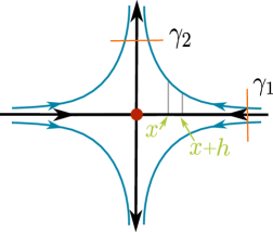
Figure 2: Central idea used to determine the time needed to pass by a saddle.

In order to construct an algorithm that is able to output an approximation, we need to estimate the time for a trajectory to pass by a saddle. We now turn to address this problem. Referring to Fig. 2, it is clear that any trajectory starting in the interior of a quadrant will stay inside the same quadrant for all $t$. Thus it suffices to consider the trajectories in the first quadrant. Since the trajectory starting at a point in the first quadrant $z_{0}=(x_{0},y_{0})$ is the graph of $z(t,z_{0})=(e^{\lambda t}x_{0},e^{\mu t}y_{0})$, it is readily seen that $t$ can be solved as a function of $x$: $t=t(x)$. Let $\gamma_{1}$ be a vertical line segment passing the point $(x_{1},0)$ and $\gamma_{2}$ a horizontal line segment passing the point $(0,y_{2})$, where $x_{1},y_{2}>0$, and let $z(t,z_{\ast})$ be the trajectory of the linear system starting at $z_{\ast}$, where $z_{\ast}=(x_{\ast},y_{\ast})$, $x_{\ast}>0$, is a point on the upper portion of $\gamma_{1}$.Then $z(t,z_{\ast})$ will stay in the first quadrant for all $t$ and cross $\gamma_{2}$ at some time instant. Assume that $z(t,z_{\ast})$ crosses $\gamma_{2}$ for the first time at $z_{\ast\ast}=(x_{\ast\ast},y_{\ast\ast})$, $x_{\ast\ast}>0$. Then this first time can be computed by the formula below: Let $T(z_{\ast})=\inf\{t>0:z(t,z_{\ast})\in\gamma_{2}\}$ be the time needed for the trajectory $z(t,z_{\ast})$ to go from $z_{\ast}$ on $\gamma_{1}$ to a point $z_{\ast\ast}=(x_{\ast\ast},y_{\ast\ast})$ on $\gamma_{2}$. Then

$$T(z_{\ast})=\int_{x_{\ast\ast}}^{x_{\ast}}\frac{dx}{\left|\lambda x\right|}$$ (13)

(see Theorem 8*.3.3 from [18, p. 221]).

Now we turn to the construction of the black box at the saddle point $0$. First we partition the ball $B(0,\varepsilon)$, which is the outer square in Fig. 3 and it will remain fixed for any application of $\mathtt{TimeEvolution}(\mathbb{D},\epsilon,T)$, into four regions: $A=\{x\in\mathbb{R}^{2}:\left\|x\right\|\leq 1/T\}$, $B=\{x\in\mathbb{R}^{2}:1/T\leq\left\|x\right\|\leq 2/T\}$, $C=\{x\in\mathbb{R}^{2}:2/T\leq\left\|x\right\|\leq 3\varepsilon/4\}$, and $D=\{x\in\mathbb{R}^{2}:3\varepsilon/4\leq\left\|x\right\|\leq\varepsilon\}$, where we assume that $2/T<3\varepsilon/4$. The region $A$ is depicted in white in Fig. 3, $B$ in yellow, $C$ in light orange, and $D$ in darker orange. Since the solution operator, $e^{Df(0)}:(t,x)\mapsto e^{Df(0)t}x$, of the linear system is computable, we are able to compute the image of (any subset or point of) $A,B,C$, or $D$ at any given time $t>0$. The neighborhood $H^{-1}_{i}(A\cup B\cup C)$ of $0$ serves as the black box.

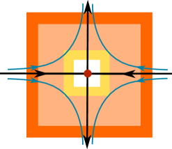
Figure 3: Vicinity of a saddle point.

Here is how the black box is programmed and incorporated with the simulation $\mathtt{TimeEvolution}$. The simulation $\mathtt{TimeEvolution}$ performs normally outside $U_{i}$ as well as in $U_{i}-H^{-1}_{i}(A\cup B\cup C)$ but stops whenever a simulated trajectory enters the black box. The linear system will then pick up a point on this simulated trajectory via $H_{i}$ as the initial point, compute the trajectory until it reaches the region $D$, and then returns a point in $D$ sufficiently close to the linear trajectory via $H^{-1}_{i}$ to $\mathtt{TimeEvolution}$; the point supplied by the black box will be $\rho/2$-close to some point on a trajectory of (2); upon receiving the answer from the black box, $\mathtt{TimeEvolution}$ resumes its normal working routine.

For a bit more details. Suppose that a trajectory computed by $\mathtt{TimeEvolution}$ enters $H_{i}^{-1}(A\cup B\cup C)$. Then we transform the system into its linearized version via the map $H_{i}$, obtaining a point $z_{j}$ in $A\cup B\cup C$. Now we compute the solution of the linear system with $z_{j}$ as the initial point, until it eventually reaches $D$. Assume that $e^{Df(0)t_{1}}z_{j}\in D$ for some $t_{1}>0$. At this moment, we pick a rational point $z_{j+1}\in D$ such that $|z_{j+1}-e^{Df(0)t_{1}}z_{j}|\leq 2^{-m(l)}$, where $m$ is a modulus of continuity for the homeomorphism $H^{-1}_{i}$ and $2^{-l}\leq\rho/2$. Then $H^{-1}_{i}(z_{j+1})\in H^{-1}_{i}(D)\subseteq U_{i}$ and $|H^{-1}_{i}(z_{j+1})-H^{-1}_{i}(e^{Df(0)t_{1}}z_{j})|\leq\rho/2$. In other words, $H^{-1}_{i}(z_{j+1})$ is an approximation with error $\rho/2$ of a point on the trajectory $\phi_{t}(\bar{x})=H^{-1}_{i}(e^{Df(0)t}z_{j})$ of (2) starting at $\bar{x}=H^{-1}_{i}(z_{j})$. Now $\mathtt{TimeEvolution}$ resumes its normal work.

There is one problem with the argument above; that is, when the point $z_{j}$ lands on the stable separatrix – the $x$ axis – of the saddle $0$. In this case, $e^{Df(0)t}z_{j}$ will stay on the stable separatrix for all $t>0$ and move towards the origin; thus it will never reach $D$. In other words, the black box won’t be able to supply an answer to $\mathtt{TimeEvolution}$ in this case. Even worse, if $z_{j}$ is on the stable separatrix or, equivalently, the $x$-coordinate of $z_{j}$ equals zero, there is in general no effective way of verifying this. The black box has to be re-programmed.

The remaining proof is devoted to re-programming the black box so that it is able to return an answer, no matter where $z_{j}$ lands in $A\cup B\cup C$. We begin by constructing, algorithmically, a finite set $J$ contained in $D$ to be used as an answer to $\mathtt{TimeEvolution}$ from the black box when $z_{j}$ is “likely” to land on the stable separatrix. Since the system is linear, it follows that, for any trajectory, if it enters $A$ along a direction other than the $x$-axis, then it will leave $A$, then $B$ and $C$, and enter $D$; in particular, once it leaves a region, it won’t re-enter that region ever again. Furthermore, for any trajectory $z(t,z_{0})=(x_{0}e^{\lambda t},y_{0}e^{\mu t})$, $y_{0}\neq 0$, if it enters $A$, $B$, $C$, or $D$, then the only way it can leave the region is through the upper or lower horizontal border of that region, because the trajectory is the graph of $x(t)=x_{0}e^{\lambda t}$ and $y(t)=y_{0}e^{\mu t}$, where $\lambda<0<\mu$. Let $m=\min_{z\in B\cup C\cup D}\|Df(0)z\|$ and $M=\max_{z\in B(0,\varepsilon)}\|Df(0)z\|$. Note that $m>0$ since $Df(0)$ is invertible and $Df(0)z=0$ has a unique solution $z=0$. Both $m$ and $M$ are computable from $f$, $\epsilon$, and $T$. Let region_H denote the union of the upper and the lower horizontal border of the region. For any point $z_{\ast}=(x_{\ast},y_{\ast})$ on $B_{H}$, the trajectory $z(t,z_{\ast})=e^{Df(0)t}z_{\ast}$ will not re-enter $B$ but leave $C$ and $D$, and eventually reach $D_{H}$. The time it takes for $z(t,z_{\ast})$ to go from $z_{\ast}$ to a point on $D_{H}$, say $z_{\ast\ast}=(x_{\ast\ast},y_{\ast\ast})$, is bounded by $3\varepsilon/m$ following (13):

$$0<\int_{x_{\ast\ast}}^{x_{\ast}}\frac{dx}{\left|\lambda x\right|}\leq\int_{0}^{3\varepsilon}\frac{dx}{m}=\frac{3\varepsilon}{m}.$$ (14)

(note that any two points in $B(0,\varepsilon)$ are within Euclidean distance $<3\varepsilon$). This time bound allows us to pick, effectively, a finite set of points with rational coordinates on $B_{H}$, $W=\{w_{1},w_{2},\ldots,w_{q}\}$, which has the following property: for every $z_{\ast}\in B_{H}$, there is some $w_{k}$ such that

$$\left\|w_{k}-z_{\ast}\right\|\leq\min\left(\frac{\varepsilon}{32e^{3\varepsilon M/m}},\frac{1}{T}\right)$$ (15)

(recall that $T$ is a rational number). Then it follows from Lemma 14 that for any $t\in[0,3\varepsilon/m]$,

$$\left\|z(t,w_{k})-z(t,z_{\ast})\right\|\leq\left\|w_{k}-z_{\ast}\right\|e^{3\varepsilon M/m}\leq\varepsilon/32$$ (16)

Without loss of generality we may assume that $\|H^{-1}_{i}(z_{1})-H^{-1}_{i}(z_{2})\|<\rho/2$ whenever $\|z_{1}-z_{2}\|\leq\varepsilon/32$. Otherwise we simply increase the precision of (15). (Recall that the modulus of continuity of $H^{-1}_{i}$ is computable.) Next pick a rational number $0<\tau<\varepsilon/(32M)$, and numerically compute $z(l\tau,w)$ for every $w\in W$ and $l=0,1,\ldots,r=\left\lfloor 3\varepsilon/(\tau m)\right\rfloor$ as long as $z((l+1)\tau,w)\in B(0,\varepsilon)$, where $\left\lfloor x\right\rfloor=\max\{n\in\mathbb{Z}:n\leq x\}$. It is clear that the following inequality holds true for any trajectory $z(t,w)$, $w\in W$:

$$\left\|z((l+1)\tau,w)-z(l\tau,w)\right\|\leq\varepsilon/32$$ (17)

Inequality (17) further implies that for each $w\in W$, there exists some $0\leq l_{w}\leq r$ such that $3\varepsilon/4+3\varepsilon/32\leq\|z(l_{w}\tau,w)\|\leq 3\varepsilon/4+5\varepsilon/32$. Finally it follows from the inequalities (15), (16), and (17) that for every $z_{\ast}\in B_{H}$, there is a $w\in W$ such that $\|z(l_{w}\tau,z_{\ast})-z(l_{w}\tau,w)\|\leq\varepsilon/32$; in particular,

$$3\varepsilon/4+\varepsilon/16\leq\|z(l_{w}\tau,z_{\ast})\|\leq 3\varepsilon/4+3\varepsilon/16$$

thus $z(l_{w}\tau,z_{\ast})\in D$. Let $J=\{z(l_{w}\tau,w):\,w\in W\}$. It follows from its construction that the finite set $J$ is computable from $f$, $\varepsilon$, and $T$.

We are now ready to re-program the black box. Proceed as before: assume that $z_{j}$ is a point in $A\cup B\cup C$ sent by $H_{i}$ and compute the trajectory $e^{Df(0)t}z_{j}$. If the numerically computed trajectory of $e^{Df(0)t}z_{j}$, with accuracy $\leq 1/T$ and using the computable version of Hartman Grobman’s theorem, does not enter $B$, then for sure the (real) trajectory $e^{Df(0)t}z_{j}$ will not enter $A$ and it will leave $C$ and then enter $D$ because the flow is linear; in this case, the black box operates as before and it will supply an answer to $\mathtt{TimeEvolution}$. On the other hand, if the numerically computed trajectory of $e^{Df(0)t}z_{j}$ enters $B$ first, the (real) trajectory $e^{Df(0)t}z_{j}$ can enter the problematic region $A$. To avoid the problem of region $A$, the black box will immediately return, as the answer to $\mathtt{TimeEvolution}$, the $H^{-1}_{i}$-image of the set $J$. It is not hard to see that the black box is now able to produce an answer whenever there is a simulated trajectory entering it because if $z_{j}$ lands on the stable separatrix of the saddle point $0$, then $e^{Df(0)t}z_{j}$ will converge to the origin and thus it will enter $A$ at some time instant and stay in $A$ thereafter.

A final note: the use of the black boxes does not affect the way how $NW(f)$ are approximated by the invariant sets of the simulation $\mathtt{TimeEvolution}$. On the one hand, the black box does not throw out any information on possible sets invariant under simulation $\mathtt{TimeEvolution}$. The only trajectory that “disappears” in the black box is the trajectory starting on the stable separatrix of the saddle; but this trajectory will move into the connected component of $Zero_{\epsilon}(f)$ containing the saddle when $T$ is large enough (or $\epsilon$ is small enough). On the other hand, for every other trajectory that enters the black box in a direction not along the stable separatrix, the black box will either supply one point in $U_{i}$ or an over-approximation $H^{-1}_{i}(J)\subset U_{i}$; in either case, every point supplied by the black box is within $\rho/2$ error bound to a point on some trajectory of (2). Since $\mathtt{TimeEvolution}$ uses $\rho/2$-grid for simulation, the invariant sets of the simulation are not going to change when the black boxes are used.

Now we come to the construction of the desired algorithm – the algorithm that computes $NW(f)$ for the full case, where saddle points may exist. The algorithm is constructed as follows: take as input $(k,f)$, where $f\in SS_{2}$ and $k\in\mathbb{N}\backslash\{0\}$ ($k$ sets the accuracy $1/k$ for the output approximation of $NW(f)$), do:

1. Let $\epsilon=1/(2k)$ and $T=1.$

2. Compute the set $Zero(f)$ with precision $1/k$ with the algorithm described in [16], obtaining an over-approximation $Zero_{\epsilon}(f)$ of $Zero(f)$. If $Zero_{\epsilon}(f)\cap\partial K\neq\varnothing$, then take $\epsilon:=\epsilon/2$, $T:=2T$, and repeat this step.

3. Compute the eigenvalues of each equilibrium in $Zero(f)$ and check whether they have opposite signs. If yes, label the equilibrium point as a saddle point.

4. If there are saddle points $z_{i}$, $i=1,\ldots,n$ compute homeomorphisms $H_{i},H_{i}^{-1}$ and $\varepsilon>0$ as stated above, and use the adapted version of $\mathtt{TimeEvolution}$.

5. Compute $\mathtt{TimeEvolution}(\mathbb{D},\epsilon,T)$ and obtain a finite set $I$ for which (12) holds.

6. Take $P=\varnothing.$

7. For each $J\subseteq I$ check if $\cup_{j\in J}B(p_{j},\epsilon/2)$ is a connected set and HasInvariantSubset$(D,\epsilon,T)=1$. If both conditions hold, take $P=P\cup\{J\}$.

8. (The minimum principle) For each $J_{1},J_{2}\in P$, test if $J_{1}\subsetneqq J_{2}$. If the test succeeds, then take $P=P\backslash\{J_{2}\}.$

9. For each $J\in P$, test if $\cup_{j\in J}B(p_{j},\epsilon)$ is contained in a connected component of $Zero_{\epsilon}(f)$. If the test succeeds, then take $P=P\backslash\{J\}.$ If the test fails but $\cup_{j\in J}B(p_{j},\epsilon)$ intersects a connected component of $Zero_{\epsilon}(f)$ containing a sink or a source, then take $\epsilon:=\epsilon/2$, $T:=2T$, and go to 2. For each $J\in P$, test if $\cup_{j\in J}B(p_{j},\epsilon)\cap\partial\mathbb{D}\neq\varnothing$. If the test succeeds, then take $\epsilon:=\epsilon/2$, $T:=2T$.

10. For each $J\in P$ and each saddle point $z_{i}$, test if $\cup_{j\in J}B(p_{j},\epsilon)$ intersects $H_{i}^{-1}(A\cup B)$ by computing the distance $d(p_{j},H_{i}^{-1}(A\cup B))$, $j\in J$, and check whether $d(p_{j},H_{i}^{-1}(A\cup B))<\epsilon$. If this is true, then take $\epsilon:=\epsilon/2$, $T:=2T$, and go to step 5.

11. Do steps 5–10 to the ODE $x^{\prime}=-f(x)$ defined over $\mathbb{D},$ i.e. by taking the transformation $t\mapsto-t$ which reverses time in (2), obtaining a set $\tilde{P}$ similar to the set $P$ of step 10.

12. For each set $J\in P\cup\tilde{P}$, use the algorithm described in Section 8.3 to check whether $\cup_{j\in J}B(p_{j},\epsilon)$ has a doughnut shape with cross-section bounded by $1/k$. If this check fails, then take $\epsilon:=\epsilon/2$, $T:=2T$, and go to step 5.

13. Check if $\mathtt{TimeEvolution}(\mathbb{D}-(Zero_{\epsilon}(f)\cup~{}\cup_{J\in P\cup\tilde{P}}(\cup_{j\in J}B(p_{j},\epsilon)),\epsilon/3,T)\subseteq Zero_{\epsilon}(f)\cup\cup_{J\in P\cup\tilde{P}}(\cup_{j\in J}B(p_{j},\epsilon))$. If this test fails, then take $\epsilon:=\epsilon/2$, $T:=2T$, and go to step 2.

14. Switch the dynamics to the ODE $x^{\prime}=-f(x)$ and test if $\mathtt{TimeEvolution}(\mathbb{D}-(Zero_{\epsilon}(f)\cup~{}\cup_{J\in P\cup\tilde{P}}(\cup_{j\in J}B(p_{j},\epsilon)),\epsilon/3,T)\subseteq Zero_{\epsilon}(f)\cup\cup_{J\in P\cup\tilde{P}}(\cup_{j\in J}B(p_{j},\epsilon/2))$ for this ODE. If this test fails, then take $\epsilon:=\epsilon/2$, $T:=2T$, and go to step 5.

15. Output $Zero_{\epsilon}(f)\bigcup\cup_{J\in P\cup\tilde{P}}\cup_{j\in J}B(p_{j},\epsilon)$.

This algorithm, with the adaptations explained above, is essentially similar to the one presented in the preceding section. A novel step that has not yet been explained is step 10. The test is designed to eliminate possible “fake” cycles which might occur when the unstable separatrix of a saddle point comes back very near to the stable separatrix. The invariant sets output by step 9 will eventually pass step 10; for the system is structurally stable and there is no saddle connection by Theorem 5. We note that since $H^{-1}_{i}:V_{i}\to U_{i}$ is a homeomorphism and $A\cup B\subset V_{i}$ is a compact set, it follows that $H^{-1}_{i}(A\cup B)$ is computable from $H^{-1}_{i}$ and $A\cup B$, and thus so is the distance $d(p_{j},H^{-1}_{i}(A\cup B))$.

8.3 Notes about the computation of limit cycles

In this section, we construct the algorithm needed for completing step 12 in the preceding algorithm. Assume that $C_{i}$ is a connected component returned from step 10 or step 11. Then $C_{i}\cap\partial\mathbb{D}=\emptyset$ and $C_{i}$ contains at least one periodic orbit, say $\gamma_{i}$. According to the Jordan Curve Theorem, $\gamma_{i}$ separates $\mathbb{R}^{2}$ into two disjoint regions, the interior (a bounded region) and the exterior (an unbounded region). The Poincaré-Bendixson Theorem further implies that there is a square $s_{i}$ (of side length $\epsilon$) containing an equilibrium point such that $s_{i}$ and $\partial\mathbb{D}$ lie in different connected components of $\mathbb{D}-C_{i}$, $s_{i}$ is in the interior while $\partial\mathbb{D}$ is in the exterior. We show that there exists a sub-algorithm that, taking as input the sets returned by steps 10 or 11, halts and outputs an approximation with an error bounded by $1/k$ of the set of all periodic orbits contained in the output approximation. The idea is to use a color-scheme algorithm to check whether $C_{i}$ is in the shape of a “doughnut” Ȯnce $C_{i}$ is confirmed to have such a shape, then the error in the approximation can be determined by measuring the width of cross sections.

As the output of step 10 or step 11 of the main algorithm presented in Section 8.2, $C_{i}$ has the form $C_{i}=\cup_{j\in J_{i}}B(p_{i,j},\epsilon)$; hence the closure of its complement, $\overline{\mathbb{D}-C_{i}}$, can be written in the form of $\overline{\mathbb{D}-C_{i}}=\cup_{j\in\bar{J}_{i}}B(\bar{p}_{i,j},\epsilon_{i,j})$, where $\bar{J}_{i}$ is a finite set of indices, $\epsilon_{i,j}$ are rational numbers satisfying $0<\epsilon_{i,j}\leq\epsilon$, and $\bar{p}_{i,j}\in\mathbb{D}$ has rational coordinates. In the following, we call $B(\bar{p}_{i,j},\epsilon_{i,j})$ a square (it can be viewed as a pixel).

The sub-algorithm embedded in step 12 of the main algorithm of Section 8.2 is defined as follows:

1. Choose a square $s$ contained in $\overline{\mathbb{D}-C_{i}}$ such that $s\cap\partial\mathbb{D}\neq\varnothing$. Paint this square $s$ blue.

2. If $s^{\prime}$ is a square contained in $\overline{\mathbb{D}-C_{i}}$ adjacent to a blue square, then paint $s^{\prime}$ blue. Repeat this procedure until there are no more squares which can be painted blue. Let $\widehat{C}_{i,blue}$ be the union of all blue squares.

3. Pick an unpainted square $\tilde{s}\subseteq Zero_{\epsilon}(f)\cap\overline{\mathbb{D}-C_{i}}$, if there is any, and paint it red.

4. If $s^{\prime}$ is a square contained in $\overline{\mathbb{D}-C_{i}}$ adjacent to a red square, then paint $s^{\prime}$ red. Repeat this procedure until there are no more squares which can be painted red. Let $\widehat{C}_{i,red}$ be the union of all red squares.

5. Let $\widehat{C}_{i}=\overline{\mathbb{D}-\widehat{C}_{i,blue}-\widehat{C}_{i,red}}$. If $\widehat{C}_{i}\cap Zero_{\epsilon}(f)\neq\varnothing$, return False (the sub-algorithm has failed).

6. Compute an overapproximation $w_{i}$ with accuracy $\epsilon$ of the quantity

   $$\max\left(\max_{x\in\widehat{C}_{i}}\min_{y\in\widehat{C}_{i,blue}}\left\|x-y\right\|,\max_{x\in\widehat{C}_{i}}\min_{y\in\widehat{C}_{i,red}}\left\|x-y\right\|\right)>0.$$ (18)

   If $2w_{i}\leq\frac{1}{k}$, then return True (the algorithm succeeded), else return False.

Note that all sets used in this sub-algorithm, $Zero_{\epsilon}(f)$, $\widehat{C}_{i,blue}$, $\partial\mathbb{D}$, $\widehat{C}_{i}$, etc., are the unions of finitely many polytopes with rational vertices. Thus, whether or not their intersections are empty can be computed in finite time.

We note that steps 1–4 are rather straightforward and can be computed in a finite amount of time. In addition, neither $\widehat{C}_{i,blue}$ nor $\widehat{C}_{i,red}$ returned by steps 1–4 is empty as shown below. Recall that $C_{i}\cap\partial\mathbb{D}=\emptyset$, $C_{i}\cap Zero_{\epsilon}(f)=\emptyset$, $C_{i}$ contains at least one periodic orbit, say $\gamma_{i}$, and $\partial\mathbb{D}$ is contained in the exterior region delimited by $\gamma_{i}$. Subsequently, $\widehat{C}_{i,blue}$ is nonempty and it does not intersect the interior of $\gamma_{i}$. If $\widehat{C}_{i,red}$ is empty, then either $Zero_{\epsilon}(f)\subseteq\widehat{C}_{i,blue}$ or there is a square in $Zero_{\epsilon}(f)$ that cannot be colored blue. If $Zero_{\epsilon}(f)\subseteq\widehat{C}_{i,blue}$, then $Zero_{\epsilon}(f)$ is contained in the exterior of $\gamma_{i}$, which is a contradiction to the Poincaré-Bendixson Theorem. Hence there is at least one square in $Zero_{\epsilon}(f)$ that cannot be colored blue. Since $C_{i}\cap Zero_{\epsilon}(f)=\emptyset$, this square is available for being picked up by step 3, which confirms that $\widehat{C}_{i,red}\neq\emptyset$.

We mention in passing that the reasoning that ensures steps 1–4 output non-empty sets $\widehat{C}_{i,blue}$ and $\widehat{C}_{i,red}$ in finite time is classical, and $\gamma_{i}$ is used in its classical capacity – its existence in $C_{i}$. In other words, the algorithm dictates computations; but the correctness of the algorithm – halting in finitely many steps with the intended output – is proved in a classical mathematical way. In the remaining of this subsection, $\gamma_{i}$ is to be used repeatedly in this capacity to show that steps 5 and 6 are guaranteed to halt with output True for sufficiently small $\epsilon$.

Next we show that if the sub-algorithm returns a True answer on input set $C_{i}$, then $C_{i}$ is ensured to be an over-approximation to the set of all periodic orbits it contains with accuracy $\leq 1/k$. Afterwards, we prove that the sub-algorithm will return True for sufficiently large $T$ and small enough $\epsilon$.

Assume that the sub-algorithm returns a True answer on input set $C_{i}$. Then every point in $\widehat{C}_{i}$ is guaranteed to be, at most, at a distance of $\leq w_{i}$ from $\widehat{C}_{i,blue}$ as well from $\widehat{C}_{i,red}$. In particular, this ensures that every point in $\widehat{C}_{i}$ will be, at most, at a distance of $\leq 2w_{i}$ from a point of $\gamma$, where $\gamma$ is an arbitrary periodic orbit contained in $\widehat{C}_{i}$. Indeed, let $x\in\widehat{C}_{i}$. Then there is some $x_{red}\in\widehat{C}_{i,red}$ and some $x_{blue}\in\widehat{C}_{i,blue}$ such that

$$\left\|x-x_{red}\right\|\leq w_{i}\text{ and }\left\|x-x_{blue}\right\|\leq w_{i}.$$ (19)

It follows from the triangular inequality that $\left\|x_{red}-x_{blue}\right\|\leq 2w_{i}$. Since $x_{red}\in\widehat{C}_{i,red}$ and $x_{blue}\in\widehat{C}_{i,blue}$, the line segment $\overline{x_{red}x_{blue}}$ will have to cross $\gamma$ at some point $y$, as to be shown momentarily. Since the line segment has length bounded by $2w_{i}$, it follows that $\left\|y-x_{red}\right\|\leq w_{i}$ or $\left\|y-x_{blue}\right\|\leq w_{i}$, which in turn implies that $\left\|x-y\right\|\leq 2w_{i}$. Consequently, we arrive at the conclusion that the Hausdorff distance between $\widehat{C}_{i}$ and the set of periodic orbits contained inside $\widehat{C}_{i}$ is at most $2w_{i}$, provided that the steps 5 & 6 of the sub-algorithm both return True answers on input $C_{i}$. Since $C_{i}\subset\widehat{C}_{i}$ by definition, the same conclusion holds true for $C_{i}$. To show that any line segment $\Sigma$ that goes from a point on $\widehat{C}_{i,blue}$ to a point on $\widehat{C}_{i,red}$ must cross each and every periodic orbit contained in $\widehat{C}_{i}$, we argue by way of a contradiction. Suppose $\gamma$ was a periodic orbit contained in $\widehat{C}_{i}$ and $\gamma\cap\Sigma=\emptyset$. Then there is a square $s$ in $Zero_{\epsilon}(f)$ lying in the interior of $\gamma$ but not colored red because $\widehat{C}_{i}\cap Zero_{\epsilon}(f)=\emptyset$ and the red region is path connected by construction (see step 4 of the sub-algorithm). Since $\widehat{C}_{i}$ does not contain any equilibrium point, it follows that each square in $Zero_{\epsilon}(f)$ is colored either blue or red and thus $s$ has color blue, which in turn implies that $s$ is in the same connected component as of $\partial\mathbb{D}$. We arrive at a contradiction, for $s$ is in the interior of $\gamma$ while $\partial\mathbb{D}$ in the exterior of $\gamma$. We have now proved that if the sub-algorithm returns a True answer on input set $C_{i}$, then $C_{i}$ is ensured to be an over-approximation to the set of all periodic orbits contained in $C_{i}$ with accuracy $\leq 1/k$.

It remains to show that the sub-algorithm will return True for sufficiently large $T$ and small enough $\epsilon$. Let $C_{i}$ be an output of step 10 or step 11 (of the main algorithm presented in section 8.2) that fails either step 5 or step 6 of the sub-algorithm. Assume that $C_{i}$ is an output of step 10, then $C_{i}$ contains at least one attractive periodic orbit named $\gamma_{i}$ as in the previous paragraphs. Our strategy is to show that, after finitely many updates on $\epsilon$, this periodic orbit $\gamma_{i}$ will be over-approximated with an error bound $1/k$ in the sense that there is a set, also called $C_{i}$ for simplicity, output by step 10 such that $\gamma_{i}$ is contained in $C_{i}$ and the sub-algorithm will output True on input $C_{i}$. Since there are only finitely many periodic orbits, the strategy ensures that, as an input to the sub-algorithm, every output of step 10 or step 11 will return True, after finitely many updates on $\epsilon$. (Recall that every output of step 10 or step 11 contains at least one periodic orbit.) The strategy is executed as follows: first, we show that $C_{i}$ will be inside a basin of attraction of $\gamma_{i}$ and $2w_{i}\leq\frac{1}{k}$ after finitely many updates on $\epsilon$ and $T$, $\epsilon:=\epsilon/2$ and $T:=2T$; second, we prove that if $C_{i}$ is inside a basin of attraction of $\gamma_{i}$, then $\widehat{C}_{i}\cap Zero_{\epsilon}(f)=\emptyset$. Hence steps 5 & 6 are guaranteed to halt with outputs True. We mention in passing that there is no need to find the exact number of updates; it suffices to show $\mathit{classically}$ that there exists a rational number such that the two mentioned conditions will be satisfied whenever $\epsilon$ is updated to be less than this rational number.

Now for the details. Assume that $C_{i}$ is an output of step 10 for some $0<\epsilon<1/(8k)$ and $T>0$. A similar argument applies to the case where $C_{i}$ is an output of step 11. Then $C_{i}$ contains at least one attractive periodic orbit, say $\gamma_{i}$.

We begin by showing that $C_{i}$ will be inside a basin of attraction of $\gamma_{i}$ and $2w_{i}<1/k$ after finitely many updates on $\epsilon$. Let $\delta_{1}>0$ be a rational number such that $\mathcal{N}_{\delta_{1}}(\gamma_{i})$ is inside a basin of attraction of $\gamma_{i}$. Pick a point $x_{0}$ on $\gamma_{i}$. Let $\Sigma\subset\mathbb{D}$ be a line segment orthogonal to $\gamma_{i}$ at $x_{0}$; i.e., let $\Sigma=\{x\in\mathbb{D}:\,(x-x_{0})\cdot f(x_{0})=0\}$. (Note that $f(x_{0})\neq 0$ since $\gamma_{i}$ cannot have any equilibrium point of (2) on it.) Then there is a rational number $0<\delta_{2}<\delta_{1}$ and a unique function $\tau(x)$, defined and continuously differentiable for $x\in\mathcal{N}_{\delta_{2}}(x_{0})$, such that $\mathcal{N}_{\delta_{2}}(x_{0})\subset\mathcal{N}_{\delta_{1}}(\gamma_{i})$, $\tau(x_{0})=T_{\gamma_{i}}=$ the period of $\gamma_{i}$, and $\phi_{\tau(x)}(x)\in\Sigma$. The restriction of $\tau$ on $\mathcal{N}_{\delta_{2}}(x_{0})\cap\Sigma$ is called the first return map or the Poincaré map. Note that $\mathcal{N}_{\delta_{2}}(x_{0})\cap\Sigma$ intersects both the interior and exterior delimited by $\gamma_{i}$. Pick two points, $y_{0}$ and $z_{0}$, on $\mathcal{N}_{\delta_{2}}(x_{0})\cap\Sigma$ such that $y_{0}$ is in the interior while $z_{0}$ is in the exterior. Let $y_{n+1}=\phi_{\tau(y_{n})}(y_{n})$ and $z_{n+1}=\phi_{\tau(z_{n})}(z_{n})$. Then the trajectory $\phi_{t}(y_{0})$ ($\phi_{t}(z_{0})$, respectively) stays in the interior (exterior, respectively) for all $t>0$ and $y_{n}\to x_{0}$ ($z_{n}\to x_{0}$, respectively) monotonically as $n\to\infty$ (see, e.g., [18, Lemma 8*.5.10,on p. 242]).

Let $t_{0}>T_{\gamma_{i}}$ be a positive number such that $Ke^{-\alpha(t_{0}-T_{\gamma_{i}})}\leq 1/(8k)$, where $T_{\gamma_{i}}$ is the period of $\gamma_{i}$. Pick an $\tilde{n}\in\mathbb{N}$ such that $\|y_{\tilde{n}}-x_{0}\|\leq 1/(8k)$, $\|z_{\tilde{n}}-x_{0}\|\leq 1/(8k)$, and

$$\min\left\{\sum_{n=0}^{\tilde{n}-1}\tau(y_{n}),\sum_{n=0}^{\tilde{n}-1}\tau(z_{n})\right\}>t_{0}$$

where

$$K=\max_{1\leq j\leq q}K_{j}\quad\mbox{and}\quad\alpha=\min_{1\leq j\leq q}\alpha_{j}/T_{j}$$ (20)

$K_{j}$, $\alpha_{j}$ and $T_{j}$ are the corresponding values of $K,\alpha,T$ provided by Proposition 7 for the periodic orbit $\gamma_{j}$. Then it follows from Proposition 7 that

$$d(\phi(t_{0}-T_{\gamma_{i}}+t,y_{0}),\gamma_{i})<1/(8k),d(\phi(t_{0}-T_{\gamma_{i}}+t,z_{0}),\gamma_{i})<1/(8k)$$

for every $t\geq 0$. Let $L_{1}$ be the trajectory of (2) from $y_{\tilde{n}}$ to $y_{\tilde{n}+1}$, $L_{2}$ the trajectory of (2) from $z_{\tilde{n}}$ to $z_{\tilde{n}+1}$, $l_{1}$ the line segment from $y_{\tilde{n}}$ to $y_{\tilde{n}+1}$, and $l_{2}$ the line segment from $z_{\tilde{n}}$ to $z_{\tilde{n}+1}$ (see Fig. 4). It is clear that $L_{1}\cup\,l_{1}$ is a simple closed curve in the interior of $\gamma_{i}$ and $L_{2}\cup l_{2}$ a simple closed curve in the exterior of $\gamma_{i}$. Since $y_{0},z_{0}\in\mathcal{N}_{\delta_{2}}(\gamma_{2})\cap\Sigma\subset\mathcal{N}_{\delta_{1}}(\gamma_{i})$ and $\mathcal{N}_{\delta_{1}}(\gamma_{i})$ is a basin of attraction of $\gamma_{i}$, it follows that the closed curves $L_{1}\cup\,l_{1}$ and $L_{2}\cup\,l_{2}$ as well the region bounded by them are contained inside $\mathcal{N}_{\delta_{1}}(\gamma_{i})$.

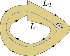
Figure 4: Curves enclosing a periodic orbit $\gamma_{i}$.

We show next that the Hausdorff distance between $L_{1}\cup l_{1}$ and $\gamma_{i}$ as well as between $L_{2}\cup l_{2}$ and $\gamma_{i}$ is bounded by $1/(8k)$. It suffices to show that $d(L_{1}\cup l_{1},\gamma_{i}(t-t_{y_{0}}))\leq 1/(8k)$ for every $T^{\prime}\leq t\leq T^{\prime}+T_{\gamma_{i}}$, where $t_{y_{0}}$ is the asymptotic phase corresponding to $y_{0}$, for some $T^{\prime}$. Two cases are to be considered:

Case (1): $\tau(y_{\tilde{n}})\geq T_{\gamma_{i}}$. In this case, by taking $T^{\prime}=\sum_{n=0}^{\tilde{n}-1}\tau(y_{n})$, for any

$$\sum_{n=0}^{\tilde{n}-1}\tau(y_{n})\leq t\leq\sum_{n=0}^{\tilde{n}-1}\tau(y_{n})+T_{\gamma_{i}}\leq\sum_{n=0}^{\tilde{n}}\tau(y_{n})$$

we have either $\phi(t,y_{0})=y_{\tilde{n}}$, or $\phi(t,y_{0})=y_{\tilde{n}+1}$, or

$$\phi(t-\sum_{n=0}^{\tilde{n}-1}\tau(y_{n}),y_{\tilde{n}})=\phi(t,y_{0})\in L_{1}$$

and

$$\|\phi(t,y_{0})-\gamma_{i}(t-t_{y_{0}})\|\leq 1/(8k)$$

Case (2): $\tau(y_{\tilde{n}})<T_{\gamma_{i}}$. Let $T_{d}$ be the positive number

$$0<T_{d}=T_{\gamma_{i}}-\tau(y_{\tilde{n}})<T_{\gamma_{i}}$$

and take $T^{\prime}=\sum_{n=0}^{\tilde{n}-1}\tau(y_{n})-T_{d}$. Then for any

$$\sum_{n=0}^{\tilde{n}-1}\tau(y_{n})-T_{d}\leq t\leq\sum_{n=0}^{\tilde{n}-1}\tau(y_{n})+T_{\gamma_{i}}-T_{d}=\sum_{n=0}^{\tilde{n}}\tau(y_{n})$$

if

$$\sum_{n=0}^{\tilde{n}-1}\tau(y_{n})\leq t\leq\sum_{n=0}^{\tilde{n}}\tau(y_{n})$$

then the proof is similar as that for case (1). On the other hand, if

$$\sum_{n=0}^{\tilde{n}-1}\tau(y_{n})-T_{d}\leq t\leq\sum_{n=0}^{\tilde{n}-1}\tau(y_{n})$$

then there exists some $1\leq m\leq\tilde{n}-1$ with

$$\sum_{n=0}^{m-1}\tau(y_{n})\leq t\leq\sum_{n=0}^{m}\tau(y_{n})$$

which implies that $\phi(t,y_{0})$ is on the trajectory somewhere between $y_{m}$ and $y_{m+1}$. Since $t\geq t_{0}-T_{\gamma_{i}}$, we also have

$$\|\phi(t,y_{0})-\gamma_{i}(t-t_{y_{0}})\|\leq 1/(8k)$$

Note that $\phi(t,y_{0})$ is not on $L_{1}\cup l_{1}$. However, since $L_{1}\cup l_{1}$ is a closed curve surrounding $\gamma_{i}$ and $y_{n}\rightarrow x_{0}$ monotonically, it follows that $L_{1}\cup l_{1}$ lies between the trajectory from $y_{m}$ to $y_{m+1}$ and $\gamma_{i}$; thus the line goes from the point $\phi(t,y_{0})$ to the point $\gamma_{i}(t-t_{y_{0}})$ must cross a point on $L_{1}$. Consequently,

$$d(L_{1}\cup l_{1},\gamma_{i}(t-t_{y_{0}}))\leq 1/(8k)$$ (21)

Define

$$\delta_{k}=\min\left\{\min_{x\in L_{1}\cup l_{1}}d(x,\gamma_{i}),\min_{x\in L_{2}\cup l_{2}}d(x,\gamma_{i}),\delta_{1}\right\}$$

Then $\delta_{k}>0$ since the compact sets $\gamma_{i}$, $L_{1}\cup l_{1}$, and $L_{2}\cup l_{2}$ are mutually disjoint. It is clear that $\mathcal{N}_{\delta_{k}}(\gamma_{i})$ is contained in $\mathcal{N}_{\delta_{1}}(\gamma_{i})$ as well in the region bounded by $L_{1}\cup l_{1}$ and $L_{2}\cup l_{2}$.

We now show that the main algorithm will output an updated $C_{i}$ that is contained in $\mathcal{N}_{\delta_{k}}(\gamma_{i})$ after finitely many updates on $\epsilon$, with the property that $2w_{i}<1/k$ and $C_{i}$ is in a basin of attraction of $\gamma_{i}$. This is indeed the case as shown as follows. Recall that the main algorithm starts with $\epsilon=1/k$ and $T=1$. With each iteration of the algorithm, the updates $\epsilon:=\epsilon/2$ and $T:=2T$ are performed. Thus, after $n$ iterations, $T=2^{n}$ and $\epsilon=1/(2^{n}k)$. Let $0<\zeta<\delta_{k}$. Then it is readily seen that the condition $2\epsilon<\zeta$ will be met after $n_{0}$ iterations with $n_{0}>1+|\log_{2}(k\zeta)|$. Similarly, for any $x\in\mathcal{N}_{\delta_{1}}(\gamma_{i})$ but $x\notin\gamma_{i}$, the condition $0<d(\phi_{t}(x),\gamma_{i})<\zeta/4$ is reached after $n_{1}$ iterations as long as $Ke^{-\alpha 2^{n_{1}}}<\zeta/4$ or, equivalently, $n_{1}>\left|\log_{2}\left(\frac{1}{\alpha}\ln\left(\frac{4K}{\zeta}\right)\right)\right|$, where $K$ and $\alpha$ are defined in (20). Note that after $n_{1}$ iterations, $T\geq 2^{n_{1}}$. Set

$$N=\max\left\{1+|\log_{2}(k\zeta)|,\left|\log_{2}\left(\frac{1}{\alpha}\ln\left(\frac{4K}{\zeta}\right)\right)\right|\right\}$$

and assume that the main algorithm is on the $n$th iteration for some $n\geq N$, and $C_{i}=\cup_{j\in J_{i}}B(p_{j},\epsilon/2)$ is an output of step 10 that contains $\gamma_{i}$. Let $\widetilde{C}_{i}=\cup\{B(p_{j},\epsilon/2):\,j\in J_{i},\,d(p_{j},\gamma_{i})\leq 3\zeta/4\}$. Then $\widetilde{C}_{i}$ covers $\gamma_{i}$. Moreover,the following are true: (i) if $x\in\widetilde{C}_{i}$, then $d(x,\gamma_{i})<\zeta$ because $\epsilon/2<\zeta/4$, which implies that $\widetilde{C}_{i}\subset\mathcal{N}_{\zeta}(\gamma_{i})\subset\mathcal{N}_{\delta_{1}}(\gamma_{i})$; (ii) if $y\in\phi_{T}(\widetilde{C}_{i})$, then $d(y,\gamma_{i})<\zeta/4$ because $T\geq 2^{n_{1}}$; and (iii) $\mathtt{TimeEvolution}(\widetilde{C}_{i},\epsilon,T)\subseteq\widetilde{C}_{i}$ (invariance of $\widetilde{C}_{i}$ by the operator $\mathtt{TimeEvolution}$). Since, by construction, $C_{i}$ is the minimal invariant set by $\mathtt{TimeEvolution}$ that includes $\gamma_{i}$, this implies that $C_{i}\subseteq\widetilde{C}_{i}$. Thus, for every $x\in C_{i}$, $d(x,\gamma_{i})<\zeta$. Therefore, $C_{i}\subseteq\mathcal{N}_{\zeta}(\gamma_{i})\subset\mathcal{N}_{\delta_{k}}(\gamma_{i})\subset\mathcal{N}_{\delta_{1}}(\gamma_{i})$. This shows that $C_{i}$ is inside the region enclosed by the closed simple curves $L_{1}\cup l_{1}$ and $L_{2}\cup l_{2}$ (we shall call it the $L$-region for simplicity), which in turn is contained in $\mathcal{N}_{\delta_{1}}(\gamma_{i})$, a basin of attraction of $\gamma_{i}$.

This suggests that if we can show that $\widehat{C}_{i}$ is contained in the $L$-region and every square in $Zero_{\epsilon}(f)$ is disjoint from the $L$-region, then $\widehat{C}_{1}\cap Zero_{\epsilon}(f)=\emptyset$. Hence step 5 returns True.

To show that $\widehat{C}_{i}$ is contained in the $L$-region, we begin with the assumption that $C_{i}\subseteq\mathcal{N}_{\delta_{k}/3}(\gamma_{i})$ and $\epsilon\leq\delta_{k}/3$. Clearly this can be done as proved above. Recall that $\mathcal{N}_{\delta_{k}}(\gamma_{i})$ is inside the $L$-region and $C_{i}$ is in the exterior of $L_{1}\cup\,l_{1}$. Then for every $x\in L_{1}\cup\,l_{1}$ or in its interior,

$$d(x,C_{i})\geq d(x,\mathcal{N}_{\delta_{k}/3}(\gamma_{i})\geq 2\delta_{k}/3\geq 2\epsilon>\epsilon.$$ (22)

We already know that there is at least one red square $s$ (of side length $\epsilon$ containing an equilibrium point $x_{e}$) in the interior of $\gamma_{i}$ and all equilibrium points in the interior of $\gamma_{i}$ must be in the interior of $L_{1}\cup\,l_{1}$ due to the fact that the $L$-region is in a basin of attraction of $\gamma_{i}$. Thus this red square covers a portion of the interior of $L_{1}\cup\,l_{1}$ and is disjoint from $C_{i}$ by (22). We shall show that $L_{1}\cup\,l_{1}$ together with its interior has color red, which implies that $\widehat{C}_{i,red}$ covers $L_{1}\cup\,l_{1}$ and its interior. It can be shown similarly that $\widehat{C}_{i,blue}$ covers $L_{2}\cup\,l_{2}$ and its exterior. This ensures that $\widehat{C}_{i}=\mathbb{D}-\widehat{C}_{i,red}-\widehat{C}_{i,blue}$ is indeed a subset of the $L$-region. We now look at the interior of $L_{1}\cup\,l_{1}$. By the Jordan curve theorem, the interior is a path-connected region and, by (22), every square with center on $L_{1}\cup\,l_{1}$ or in its interior having side length $\epsilon$ is disjoint from $C_{i}$. Then step 4 of the subalgorithm colors every such square red starting with the red square containing $x_{e}$. Since each square in $Zero_{\epsilon}(f)$ has side-length $\epsilon$ and contains one equilibrium point either in the interior of $L_{1}\cup\,l_{1}$ or in the exterior of $L_{1}\cup\,l_{2}$, it follows that $Zero_{\epsilon}(f)\subset\widehat{C}_{i,red}\cup\,\widehat{C}_{i,blue}$. Hence $\widehat{C}_{i}\cap Zero_{\epsilon}(f)=\emptyset$.

Finally, it follows from (21) that $d(\widehat{C}_{i},\gamma_{i})\leq 1/(8k)$. Hence the quantity (18) is bounded by $1/(4k)$. We recall that $w_{i}$ is an over-approximation of the quantity (18) with an error bound $\epsilon\leq 1/(8k)$. This implies that $w_{i}<1/(2k)$ or, equivalently, $2w_{i}<1/k$. Thus step 6 also returns True. The proof is complete.

We conclude this section with the computation of a cross-section for each $\widehat{C}_{i}$, where $\widehat{C}_{i}$ is the output of a successful run of the subalgorithm, $i$ is in some finite index set $I$, and $\bigcup_{i\in I}C_{i}$ is an over-approximation of $Per(f)$ with error bound $1/k$. Recall that a cross-section of $\widehat{C}_{i}$ is a line segment that lies in $\widehat{C}_{i}$, is transversal to all trajectories across it, and intersects with all periodic orbits contained in $\widehat{C}_{i}$. These cross-sections will be used in the next section for computing the exact number of periodic orbits contained in $C_{i}$. The same technique used to write the subalgorithm can be extended to compute the desired cross-sections.

Given $C_{i}$, let $\widehat{C}_{i}$, $\widehat{C}_{i,red}$, $\widehat{C}_{i,blue}$ be the corresponding sets obtained by a successful run of the preceding subalgorithm, $i\in I$. Then to compute a cross-section for $\widehat{C}_{i}$, proceed as follows:

1. Compute a rational point $p_{i}$ on $\widehat{C}_{i}\cap\widehat{C}_{i,red}$ (it suffices to look at the vertices of the finitely many squares which form $\widehat{C}_{i}$ and pick one such vertex which is also painted red. Note that all the vertices of the squares defining $\widehat{C}_{i}$ and $\widehat{C}_{i,red}$ have rational coordinates, and therefore such a $p_{i}$ can be computed in finite time).

2. Consider the vector $n(p_{i})=(-f_{2}(p_{i}),f_{1}(p_{i}))$ which is orthogonal fo $f(p_{i})\neq 0$. Compute a rational approximation $v_{i}$ to $n(p_{i})$ with accuracy bounded by $\epsilon$.

3. Test whether $\measuredangle(v_{i},n(p_{i}))\leq\pi/10$ or $\measuredangle(v_{i},n(p_{i}))\geq\pi/11$, where $\measuredangle(x,y)$ denotes the positive angle between vectors $x$ and $y$. If $\measuredangle(v_{i},n(p_{i}))\geq\pi/11$, then update $\epsilon:=\epsilon/2$ and go to step 2.

4. Let $s_{1},\ldots,s_{l}$ be the squares (with rational vertices) computed by the preceding subalgorithm such that $\widehat{C}_{i,blue}=\cup_{j=1,\ldots,l}s_{j}$; let $l_{v_{i}}$ be the ray starting at $p_{i}$ and parallel to $v_{i}$ such that $p_{i}$ is the only red point on $l_{v_{i}}$. Starting from $j=1$, for each $1\leq j\leq l$, decide whether $s_{j}\cap l_{v_{i}}\mathbb{=\varnothing}$. If the condition holds true, take $r_{j}$ being the point $(3,0)$ in $\mathbb{R}^{2}$ and move to $s_{j+1}$. If $s_{j}\cap l_{v_{i}}\neq\emptyset$, compute the point $r_{j}\in\mathbb{D}$ (which has rational coordinates) satisfying $\left\|r_{j}-p_{i}\right\|=\min_{y\in s_{j}\cap l_{v_{i}}}\left\|y-p_{i}\right\|$, and then move to $s_{j+1}$. (We note that, in the latter case, $r_{j}$ is a blue point.)

5. Take $q_{i}$ be some $r_{j}$ satisfying $\left\|q_{i}-p_{i}\right\|=\min_{j=1,\ldots,l}\left\|r_{j}-p_{i}\right\|$.

6. Compute

   $$\theta=\max_{z\in\overline{p_{i}q_{i}}}\measuredangle(f(p_{i}),f(z))=\left|\arccos\left(\frac{f(p_{i})\cdot f(z)}{\left\|f(p_{i})\right\|\left\|f(z)\right\|}\right)\right|$$

   and test whether $\theta\leq\pi/10$ or $\theta\geq\pi/11$. If $\theta\geq\pi/11$, then update $\epsilon:=\epsilon/2$ and $T:=2T$ in the main algorithm of Section 8.2, obtaining new sets $C_{i}$, $\widehat{C}_{i},$ $\widehat{C}_{i,red},$ $\widehat{C}_{i,blue}$ and repeat the current algorithm starting from step 1.

7. Output the line segment $\overline{p_{i}q_{i}}$ as a cross-section for $\widehat{C}_{i}$.

We need to show that the algorithm halts after finitely many updates on $\epsilon$; when it halts, it returns a cross-section of $\widehat{C}_{i}$. The first five steps are rather straightforward, for $f(p_{i})$ is computable and every square in $\widehat{C}_{i,red}$ or $\widehat{C}_{i,blue}$ has rational corners and rational side-length. Since the ray $l_{v_{i}}$ starting from the red point $p_{i}$ will move out of $\mathbb{D}$, it must cross the blue -colored $\partial\mathbb{D}$. Hence, there is at least one square, say $s_{j}$, in $\widehat{C}_{i,blue}$ such that $s_{j}\cap l_{v_{i}}\neq\emptyset$. This ensures that $q_{i}$ has color blue and the length of $\overline{p_{i}q_{i}}>0$ (recall that $\widehat{C}_{i,red}\cap\widehat{C}_{i,blue}=\emptyset$). We now turn to step 6. We begin with the definition of the function

$$h:\bigcup_{i\in I}\widehat{C}_{i}\times\bigcup_{i\in I}\widehat{C}_{i}\rightarrow\mathbb{R},\quad h(x,y)=\measuredangle(f(x),f(y))=\arccos\left(\frac{f(x)\cdot f(y)}{\left\|f(x)\right\|\left\|f(y)\right\|}\right)$$

For simplicity, we call $\bigcup_{i\in I}\widehat{C}_{i}$ a hat-over-approximation of $Per(f)$. Since $\bigcup_{i\in I}\widehat{C}_{i}$ is a compact subset of $\mathbb{D}$ and $\widehat{C}_{i}\cap Zero_{\epsilon}(f)=\emptyset$ for all $i\in I$, the function $h$ is well-defined and uniformly continuous on $\bigcup_{i\in I}\widehat{C}_{i}\times\bigcup_{i\in I}\widehat{C}_{i}$. Thus, there is a rational number $\delta>0$ such that

$$|h(x_{1},y_{1})-h(x_{2},y_{2})|<\pi/10\quad\mbox{whenever}\quad\|(x_{1},y_{1})-(x_{2},y_{2})\|\leq\delta$$ (23)

Hence, if the length of $\overline{p_{i}q_{i}}$ is no larger than $\delta$, then $\theta\leq\pi/10$. On the other hand, suppose the length of $\overline{p_{i}q_{i}}$ is larger than $\delta$. In this case, we recall briefly some facts which were worked out in detail in the proof of the preceding subalgorithm. First, when $\epsilon$ and $T$ are updated, the updated hat-over-approximation is a subset of the hat-over-approximation before the update. This indicates that (23) holds true for any updated hat-over-approximation. Second, given any positive integer $l$, the main algorithm of section 8.2 and the preceding subalgorithm can output a hat-over-approximation such that $w_{i}+\epsilon<1/l$ for all $i$ by updating $\epsilon$ and $T$ finitely many times, where $w_{i}$ is an approximation with accuracy $\epsilon$ to the quantity defined in (18). Hence, by picking $l$ such that $(1/l)<\delta$ and by updating $\epsilon$ and $T$, the condition $w_{i}+\epsilon<\delta$ is ensured to be met for all $i$. Now since the length of $\overline{p_{i}q_{i}}$ cannot be larger than $w_{i}+\epsilon$ by definition of $q_{i}$, it follows that the length of $\overline{p_{i}q_{i}}$ will be bounded by $\delta$ for all $i$ after updating $\epsilon$ and $T$ finitely many times. Hence, step 6 will halt and output $\theta\leq\pi/10$. As the last step, we show that $\overline{p_{i}q_{i}}$ is indeed a cross-section of $\widehat{C}_{i}$. It is clear that $\overline{p_{i}q_{i}}$ lies in $\widehat{C}_{i}$. We recall that it has been shown in the proof of the preceding subalgorithm that any line segment that goes from a point on $\widehat{C}_{i,red}$ to a point on $\widehat{C}_{i,blue}$ must cross each and every periodic orbit contained in $\widehat{C}_{i}$. It remains to show that the trajectories move through $\overline{p_{i}q_{i}}$ transversely at every point on $\overline{p_{i}q_{i}}$. For any $z\in\overline{p_{i}q_{i}}$, since $\measuredangle(f(p_{i}),f(z))\leq\theta\leq\pi/10$ and $\measuredangle(v_{i},n(p_{i}))\leq\pi/10$, it follows that $\measuredangle(f(z),v_{i})\geq\measuredangle(f(p_{i}),n(p_{i}))-\measuredangle(n(p_{i}),v_{i})-\measuredangle(f(p_{i}),f(z))\geq(\pi/2)-(\pi/10)-(\pi/10)=3\pi/10$. Hence, the trajectories cross $\overline{p_{i}q_{i}}$ transversely at every point on $\overline{p_{i}q_{i}}$.

9 Computing Poincaré maps

In this section, we make use of Poincaré maps (or first return maps) to construct an algorithm for computing the number of periodic orbits contained in each $C_{i}$. A cross-section is needed in order to define a first return map. Since we have an algorithm for computing a corss-section of $\widehat{C}_{i}$, it is natural to work with $\widehat{C}_{i}$ instead of $C_{i}$ provided that $\widehat{C}_{i}$ is invariant for all $t\geq T$ for some $T>0$ and $\widehat{C}_{i}\cap\widehat{C}_{j}=\emptyset$ whenever $i\neq j$. The first condition guarantees that the first return map can be defined in a neighborhood of a cross-section when $T$ is sufficiently large, and the second condition ensures that $\widehat{C}_{i}$ contains the exact number of periodic orbits as $C_{i}$ does because $C_{i}\subseteq\widehat{C}_{i}$ and $Per(f)\subset\cup_{i}C_{i}$.

We give a sketch that both conditions shall be met. Suppose $\widehat{C}_{i}$, $i\in I$, are True outcomes of the subalgorithm with input parameters $\epsilon$ and $T$. Now compute HasInvariantSubset$(\widehat{C}_{i},\epsilon,T)$ and test whether $\widehat{C}_{i}\cap\widehat{C}_{j}=\emptyset$. If HasInvariantSubset$(\widehat{C}_{i},\epsilon,T)=1$ for all $i$ and $\widehat{C}_{i}\cap\widehat{C}_{j}=\emptyset$ whenever $i\neq j$, then return True. Otherwise, update $\epsilon:=\epsilon/2$ and $T:=2T$ and rerun the main- and the sub-algorithm. It can be proved that the computation and the test will return True after finitely many updates on $\epsilon$ and $T$ by an argument similar to that used to confirm that steps 5 and 6 in the subalgorithm will return True after finitely many updates on $\epsilon$ and $T$.

In the remainder of this section, we assume that $\widehat{C}_{i}$ are the True returns and $Per(f)\subset\cup_{i}\widehat{C}_{i}$. For simplicity, we further assume that $\widehat{C}_{i}$ is invariant for all $t>0$ by a transformation of time. For each $\widehat{C}_{i}$, let $\overline{p_{i}q_{i}}$ be the cross-section of $\widehat{C}_{i}$ computed at the end of the previous section. Then a Poincaré map $P_{i}$ can be defined on $\overline{p_{i}q_{i}}$: it assigns to every $p$ on $\overline{p_{i}q_{i}}$ the point on $\overline{p_{i}q_{i}}$ that is first reached by following the trajectory $\phi_{t}(p)$ for $t>0$. In particular, a point $q$ on $\overline{p_{i}q_{i}}$ is on a periodic orbit iff $q$ is a fixed point of the Poincaré map, $P_{i}(q)=q$. Hence, in order to compute the number of periodic orbits contained in $\widehat{C}_{i}$, we just need to compute the number of fixed points of $P_{i}$ or, equivalently, the number of zeros of the function $Q_{i}:\overline{p_{i}q_{i}}\rightarrow\mathbb{R}^{2}$ defined by $Q_{i}(x)=P_{i}(x)-x$. The number of zeros of $Q_{i}$ can be computed using the algorithm from Section 6 as long as $Q_{i}$ has the following properties:

1. If $q$ is a zero of $Q_{i}$, then the jacobian of $Q_{i}$ at point $q$, $DQ_{i}(q)$, is invertible;

2. $Q_{i}$ and $DQ_{i}$ are computable from $f$ of (2).

It is well known that if all periodic orbits in $C_{i}$ are hyperbolic, then condition 1 holds.

Concerning condition 2, it suffices to show that the Poincaré map $P_{i}$ and its derivative $DP_{i}$ are computable from $f$.

Theorem 22

Let $\Sigma=\overline{p_{i}q_{i}}\subseteq\mathbb{D}\subseteq\mathbb{R}^{2}$ be a computable line segment which defines a cross-section for a periodic orbit $\gamma$ of (2), where $f\in C^{1}(\mathbb{D})$. Suppose also that the Poincaré map $P:\Sigma\rightarrow\Sigma$ is defined for all all points $x\in\Sigma$. Then $P$ and $DP$ are computable from $f$ of (2).

Proof. The techniques from [12] and [37] are used to prove the computability of $P$ and $DP$, respectively.

We begin by showing that $P$ is computable. Since $\Sigma=\overline{p_{i}q_{i}}$ is a cross-section on an approximation $\widehat{C}_{i}$ of some periodic orbit(s), the flow of (2) crosses this section transversaly. This implies that for any point $x\in\Sigma$, the angle $\measuredangle(f(x),\Sigma)$ between $f(x)$ and $\Sigma$ is nonzero, $\measuredangle(f(x),\Sigma)>0$. Let $\theta=\frac{\min_{x\in\Sigma}\measuredangle(f(x),\Sigma)}{2}>0$. Then $\theta$ is computable from $f$. Furthermore, by continuity of $f$, there exists some $\varepsilon>0$ such that

$$\min_{x\in B(\Sigma,\varepsilon)}\measuredangle(f(x),\Sigma)>\theta>0$$

where $B(\Sigma,\varepsilon)=\{x\in\mathbb{D}:\left\|y-x\right\|\leq\varepsilon$ for some $y\in\Sigma\}$ contains no zeros of $f$. Let

$$\alpha=\min_{x\in B(\Sigma,\varepsilon)}\left\|f(x)\right\|,\text{ \ \ }\beta=\max_{x\in B(\Sigma,\varepsilon)}\left\|f(x)\right\|$$

Since $B(\Sigma,\varepsilon)$ is compact and contains no zero of $f$, it follows that $\alpha,\beta>0$. It is convenient to view $B(\Sigma,\varepsilon)$ as a rectangle. Note that $B(\Sigma,\varepsilon)\cap\widehat{C}_{i}$ is divided into two parts $B_{1}$ and $B_{2}$ by the line passing through $p_{i}$ and $q_{i}$. Let us assume, without loss of generality, that the flow passes from $B_{1}$ through $\Sigma$ and then moves through $B_{2}$ until it leaves $B(\Sigma,\varepsilon)$. A simple analysis shows that the flow of (2) cannot take more than $2\varepsilon/(\alpha\sin\theta)>0$ time units to cross $B(\Sigma,\varepsilon)$ (the flow will have to cross this rectangle; but since the norm of the orthogonal component is at least $\alpha\sin\theta$, this will be done in time $2\varepsilon/(\alpha\sin\theta)$), but requires at least $2\varepsilon/\beta>0$ time units to cross it (because the norm of the orthogonal component is bounded by $\beta$). Therefore if $x$ and $y$ are solutions of (2) with initial conditions $x(0)=x_{0}$ and $y(0)=y_{0}$, with $x_{0},y_{0}\in B(\Sigma,\varepsilon)\cap\widehat{C}_{i}$, then $x(t)$ and $y(t)$ leave $B(\Sigma,\varepsilon)$ at times $t_{x},t_{y}\in[0,2\varepsilon/(\alpha\sin\theta)]$, respectively.

Now take some rational $\varepsilon_{0}>0$ satisfying $\varepsilon_{0}\leq\min\{\epsilon\alpha\sin\theta/2,\varepsilon\}$, where $\epsilon>0$ is a rational yet to be defined. In particular, this implies that the time for the flow in $\widehat{C}_{i}$ to cross $B(\Sigma,\varepsilon_{0})\subseteq B(\Sigma,\varepsilon)$ is bounded by

$$2\varepsilon_{0}/(\alpha\sin\theta)\leq\frac{2\epsilon\alpha\sin\theta}{2\alpha\sin\theta}\leq\epsilon$$ (24)

Let $\bar{B}_{1}=B_{1}\cap B(\Sigma,\varepsilon_{0})$, $\bar{B}_{2}=B_{2}\cap B(\Sigma,\varepsilon_{0})$, and $\delta=\varepsilon_{0}/(2\beta)$. Next consider the sequence of iterates $\phi_{t_{i}}(x)$, where $x\in\Sigma$, $0<t_{i+1}-t_{i}\leq\delta$, and $\{t_{i}\}_{i\in\mathbb{N}}$ is computable. Since the flow $\phi_{t}(x)$ takes at least $2\delta$ time units to cross each band $\bar{B}_{1}$ or $\bar{B}_{2}$, we are certain that $\phi_{t_{1}}(x),\phi_{t_{2}}(x)\in\bar{B}_{2}$ when the flow first leaves $\Sigma$ from $x$ and that there is some $k>0$ such that $\phi_{t_{k}}(x),\phi_{t_{k+1}}(x)\in\bar{B}_{1}$ with $t_{k},t_{k+1}>t_{1}>0$. Note that, at most, only one of the iterates $\phi_{t_{k}}(x),\phi_{t_{k+1}}(x)$ are on $\partial\bar{B}_{1}$, so that at least one of the iterates $\phi_{t_{k}}(x),\phi_{t_{k+1}}(x)$ is in the interior of $\bar{B}_{1}$. Since $\bar{B}_{1}$ is compact and computable, so does the closure of its complement. Thus, we can decide whether one of the iterates $\phi_{t_{k}}(x),\phi_{t_{k+1}}(x)$ is on $\bar{B}_{1}$ or on the closure of its complement (the problematic case to detect is when one of these iterates is on $\partial\bar{B}_{1}$, and that’s why we always use two iterates, since this ensures that at least one of the iterates will not be on the boundary of $\bar{B}_{1}$). If we conclude that one iterate is on the closure of the complement of $\bar{B}_{1}$, then we skip this iteration and increment $k$ until (and that will eventually happen) it reaches the first $k$ for which we conclude that $\phi_{t_{k}}(x)$ belongs to $B(\Sigma,\varepsilon_{0})$ and thus also necessarily to $\bar{B}_{2}$ and then return $\phi_{t_{k}}(x)$.

Now we turn to find some sufficiently small $\epsilon>0$ such that $\phi_{t_{k}}(x)$ is close enough to the real value $P(x)$. Assume that we need to compute $P(x)$ with accuracy $2^{-j}$ for some $j>0$. Recall that the time needed for the flow in $\widehat{C}_{i}$ to cross $B(\Sigma,\varepsilon_{0})$ is bounded by (24). Hence, the time it takes to cross $\bar{B}_{1}$ until reaching $\Sigma$ is bounded by $\epsilon/2$. Let $M$ be a rational such that $M\geq\sup_{x\in\bar{B}_{1}}\left\|f(x)\right\|$, which is computable from $f$. Then $\left\|P(x)-\phi_{t_{k}}(x)\right\|\leq M\epsilon/2$. Furthermore, since we usually cannot compute $\phi_{t_{k}}(x)$ exactly, but only an approximation $\bar{\phi}_{t_{k}}(x)$ of it, it follows that if we take $\epsilon\leq 2^{-j}/M$ and compute $\bar{\phi}_{t_{k}}(x)$ with accuracy bounded by $M\epsilon/2$, then we have

$$\left\|P(x)-\bar{\phi}_{t_{k}}(x)\right\| \leq\left\|P(x)-\phi_{t_{k}}(x)\right\|+\left\|\phi_{t_{k}}(x)-\bar{\phi}_{t_{k}}(x)\right\|$$

$$\leq M\epsilon/2+M\epsilon/2$$

$$\leq M\epsilon$$

$$\leq 2^{-j}$$

It remains to show that $DP$ is computable. The proof essentially follows along the lines of [37, Section 5] and uses the fact just shown above that $P$ is computable. We may assume that the (computable) cross-section $\Sigma$ is parallel to the vertical axis. If the asumption is not true, a (computable) change of basis will result in the desirable case.

First we note that if $\phi(t,\bar{x})$ denotes the solution of (2) with initial condition $x(0)=\bar{x}$ at time $t$, and if given some $x\in\Sigma$, $\tau(x)>0$ denotes the first time where the trajectory starting on $x\in\Sigma$ will hit $\Sigma$ again, we have $P(x)=\phi(\tau(x),x)$. Let us now calculate the partial derivatives of $P=(P_{1},P_{2})$. We have

$$\frac{\partial P_{i}}{\partial x_{j}}(x) =\frac{\partial}{\partial x_{j}}\phi_{i}(\tau(x),x)$$

$$=\frac{\partial\phi_{i}(\tau(x),x)}{\partial t}\frac{\partial\tau(x)}{\partial x_{j}}+\frac{\partial\phi_{i}(\tau(x),x)}{\partial x_{j}}$$

$$=f_{i}(\phi(\tau(x),x))\frac{\partial\tau(x)}{\partial x_{j}}+\frac{\partial\phi_{i}(\tau(x),x)}{\partial x_{j}}$$

$$=f_{i}(P(x))\frac{\partial\tau(x)}{\partial x_{j}}+\frac{\partial\phi_{i}(\tau(x),x)}{\partial x_{j}}$$ (25)

for $i=1,2$. To obtain the partial derivatives of $\tau(x)$, we note that $P_{1}(x)$ is constant. Hence, by (25)

$$0=\frac{\partial P_{1}}{\partial x_{j}}(x)=f_{1}(P(x))\frac{\partial\tau(x)}{\partial x_{j}}+\frac{\partial\phi_{1}(\tau(x),x)}{\partial x_{j}}.$$

Solving for $\partial\tau(x)/\partial x_{j}$, we get

$$\frac{\partial\tau(x)}{\partial x_{j}}=-\frac{\partial\phi_{1}(\tau(x),x)}{\partial x_{j}}\frac{1}{f_{1}(P(x))}$$

(note that $f_{1}(P(x))\neq 0$ as the flow of (2) is transverse to $\Sigma$). Replacing this last expression into (25) (note that we only need to compute the partial derivatives of $P_{2}$ as the partial derivatives of $P_{1}$ are zero, as we have seen), we get

$$\frac{\partial P_{2}}{\partial x_{j}}(x)=-f_{2}(P(x))\frac{\partial\phi_{1}(\tau(x),x)}{\partial x_{j}}\frac{1}{f_{1}(P(x))}+\frac{\partial\phi_{2}(\tau(x),x)}{\partial x_{j}}$$ (26)

The only element still missing in order to compute the partial derivatives of $P_{2}$ is the computation of the partial derivatives of $\phi_{l}$, for $l=1,2$. This can be achieved as follows. From (2) we get that $\left(\phi_{k}(t,x)\right)^{\prime}=f_{k}(\phi(t,x))$ for $k=1,2$. By applying partial derivatives to both sides and switching the order of differentiation on the left-hand side ($\phi$ is $C^{2}$ and thus this operation will not affect the result), we get

$$\frac{d}{dt}\frac{\partial\phi_{l}(t,x)}{\partial x_{j}}=\sum_{i=1}^{2}\frac{\partial f_{l}}{\partial x_{i}}(\phi(t,x))\frac{\partial\phi_{i}}{\partial x_{j}}(t,x)\text{, }l=1,2.$$

In matrix form this can be written as

$$\frac{d}{dt}D\phi(t,x)=Df(\phi(t,x))D\phi(t,x)$$

which is a linear ODE with the initial condition $D\phi(0,x)=I$ (note that $\phi(0,x)=x$ is the identity map and that the partial derivatives are only taken in order to $x$). The solution of this initial-value problem can be computed as the solution of an ODE, for an arbitrary amount of time as in [14]. Moreover the time $\tau(x)$ used in (26) can also be computed as in [12]. Indeed, from the above arguments, one can conclude that to compute $\tau(x)$ with accuracy $2^{-n}$ it suffices to take $\epsilon<2^{-n}$ and return $t_{k}$ as above. This proves the theorem.   

10 Proof of Theorem B – Putting it all together

Let us assume that $Zero_{\epsilon}(f)$ does not include any (very small) periodic orbit. This can be ensured, for example, by using Theorem 21, the computable Hartman-Grobman theorem, to compute some $\epsilon>0$ such that if $x_{0}$ is an equilibrium point, then $B(x_{0},\epsilon)$ is inside the neighborhood computed by the computable version of the Hartman-Grobman Theorem. In this neighborhood there are no periodic orbits, since the flow is conjugated to a linear flow there, and therefore periodic orbits can only exist on the doughnut-like sets computed in previous sections.

These doughnut-like sets thus include all the periodic orbits with arbitrarily high accuracy. We have also shown that on each of these doughnut-like sets we can define a cross-section and compute a Poincaré map, $P$, there. Moreover, using the technique of Section 6 we can compute the number of zeros of $P(x)-x$, i.e. the number of fixed points of $P$. But the number of fixed points is equal to the number of periodic orbits. Hence Theorem B is proved.

11 Connections with Hilbert’s 16th problem

The algorithm constructed in Theorem B computes the positions and the exact number of the periodic orbits for every vector field in $SS_{2}$. Let us call the algorithm Algo. As a by-product, Algo produces a computable function $\phi:SS_{2}\to\mathbb{N}$, where $\phi(f)=$ the number of the periodic orbit(s) of $f$ on $\mathbb{D}$. The pre-images of $\phi$ decompose $SS_{2}$ into mutually disjoint open connected components $C_{j}$, $j\in\mathbb{N}$. Let $\mathcal{P}$ (respectively, $\mathcal{P}_{\mathbb{Q}}$) denote the set of all polynomials (respectively, all polynomials with rational coefficients) defined on $\mathbb{D}$. Then $\mathcal{P}_{\mathbb{Q}}$ is dense in $C^{1}(\mathbb{D})$. Since $SS_{2}$ is an open subset of $C^{1}(\mathbb{D})$, it follows that every $C_{j}$ contains (infinitely many) polynomials from $\mathcal{P}_{\mathbb{Q}}$. Hence, if there is an algorithm, say A-for-H (an algorithm for Hilbert’s 16th problem), that computes an upper bound $u(n)$ for the numbers of periodic orbits of polynomials of degree $n$ in $SS_{2}\bigcap\mathcal{P}_{\mathbb{Q}}$, then $u(n)$ is also an upper bound for the numbers of periodic orbits of all polynomials of degree $n$ in $SS_{2}$. This result would provide an affirmative answer to Hilbert’s 16th problem restricted to polynomials in $SS_{2}$, that is, the structurally stable polynomials on $\mathbb{D}$. Since $SS_{2}$ is an open dense subset in $C^{1}(\mathbb{D})$, a property true on $SS_{2}$ is typical and generic.

Whether an A-for-H algorithm exists is an open problem. Theorem C indicates that one may not be able to construct algorithms of an A-for-H nature but for computing sharp upper bounds over certain classes of polynomial systems. On the other hand, we construct in the following an A-for-H algorithm over $SS_{2}\bigcap\mathcal{P}$ that works relative to the Halting problem. In other words, it is possible to devise a Turing machine (an algorithm) that solves Hilbert’s 16th problem over $SS_{2}\bigcap\mathcal{P}$, provided that the Halting problem

$$HALT=\{(M,i):\text{the Turing machine $M$ halts with input }i\}$$

is given as an oracle. As usual, we use the notation $C\leq HALT$ to denote that the problem $C$ is solvable by an algorithm that works relative to the halting problem (or, more generally, relative to another problem).

We begin by effectively listing the polynomial systems in $\mathcal{P}_{SS_{2}}=SS_{2}\bigcap\mathcal{P}_{\mathbb{Q}}$. First we note that $\mathcal{P}_{\mathbb{Q}}$ can be enumerated as $\mathcal{P}_{\mathbb{Q}}=\{P_{j}\}_{j=1}^{\infty}$. Let $M$ be a Turing machine that on input $k$ computes the first $k$ steps of Algo$(P_{1})$, Algo$(P_{2})$, $\ldots$, Algo$(P_{k})$. $M(k)$ outputs $P_{j}$ if $1\leq j\leq k$, Algo$(P_{j})$ halts in $\leq k$ steps, and $P_{j}$ is not the output of $M(l)$ for $l<k$; otherwise, $M(k)$ outputs the empty set. It is clear that $M$ lists recursively all polynomial systems in $SS_{2}\bigcap\mathcal{P}_{\mathbb{Q}}$. For simplicity, we use $\{P_{j}\}$ to denote this computable sequence. Then $\{P_{j}\}$ is a subset of $\mathcal{P}\bigcap SS_{2}$.

Let $\mathcal{A}\subseteq\mathcal{P}$ and let $Hilbert_{16}(\mathcal{A})$ be the problem of solving the Hilbert’s 16th problem over the set $\mathcal{A}$, i.e.  computing an upper bound for the numbers of periodic orbits of all elements of $\mathcal{A}$ of degree $n$, where $n$ is given as an input.

Theorem 23

$Hilbert_{16}(\mathcal{P}\cap SS_{2})\leq HALT$.

Proof. Consider the Turing machines $N_{n}$, $n\in\mathbb{N}\setminus\{0\}$, defined as follows, where $k\in\mathbb{N}$ is the input of $N_{n}$:

1. Let $i=1$.

2. Consider the polynomial vector fields with rational coefficients $P_{1},P_{2},\ldots,P_{i}$ (in $\mathcal{P}_{SS_{2}}$) and retain only those which have degree $n$. For each of the retained polynomial vector fields, use it as an input to the algorithm Algo, but simulate only $i$ steps of the algorithm. If in any of these computations the algorithm Algo stops and returns a number greater than or equal to $k$, then $N_{n}$ stops its computation. Otherwise, $i$ is incremented and Step 2 is repeated.

It is clear that $N_{n}$ halts on input $k$ only if there is a vector field in $\{P_{j}\}$ with $k$ or more periodic orbits. Otherwise $N_{n}$ will not halt with input $k$.

Now consider the Turing machine that has oracle access to $HALT$ defined as follows: on input $n$ (the degree of the polynomials),

1. Set $k=1$.

2. Using the oracle to decide whether $(N_{n},k)\in HALT$. If the answer is positive, then increment $k$ and repeat this step. Otherwise return $k$.

It is readily seen that the output of this Turing machine on input $n$ would provide a (sharp) upper bound for the numbers of periodic orbits of polynomials of degree $n$ in $\{P_{j}\}$, provided that such a bound exists. In the case that the upper bound doesn’t exist, the Turing machine won’t halt.

As we mentioned at the beginning of this section, an upper bound for the numbers of periodic orbits of polynomials of degree $n$ in $\{P_{j}\}$ is also an upper bound of the same nature of polynomials of degree $n$ in $\mathcal{P}\bigcap SS_{2}$.   

The result above can be generalized from the compact domain $\mathbb{D}$ to $\mathbb{R}^{2}$. Now let $\mathcal{P}$ denote the set of polynomial vector fields defined over the whole plane $\mathbb{R}^{2}$, and let $\mathcal{P}_{m}$ denote the set of polynomial vector fields of degree $m$. Then we have:

Theorem 24

There are dense subsets $A,B$ of $\mathcal{P}$, where $B$ is also open, such that $B\subseteq A\subseteq\mathcal{P}$ and $Hilbert_{16}(A)\leq HALT$.

Proof. The proof of this result is similar to the previous theorem, but some adaptations are needed. In [32, Theorem 4, p. 327] it is mentioned that the set $\mathcal{B}_{m}$ of polynomial vector fields of degree $m$ which are structurally stable on $\mathbb{R}^{2}$ under $C^{1}$-perturbations is open and dense in $\mathcal{P}_{m}$. Furthermore, every system in $\mathcal{B}_{m}$ only has hyperbolic equilibrium points/periodic orbits without any saddle connections even if it has saddles at infinity. Let $\mathcal{A}_{m}$ be the systems in $\mathcal{P}_{m}$ which (i) only have hyperbolic equilibrium points and periodic orbits, and (ii) have no “finite” saddle connections but may have saddle connections involving saddles at infinity. It is clear that $\mathcal{B}_{m}\subseteq\mathcal{A}_{m}\subseteq\mathcal{P}_{m}$; thus $\mathcal{A}_{m}$ is also dense in $\mathcal{P}_{m}$. Let $\mathcal{A}=\cup_{m\in\mathbb{N}}\mathcal{A}_{m}$ and $\mathcal{B}=\cup_{m\in\mathbb{N}}\mathcal{B}_{m}$. Then $\mathcal{B}$ is open, $\mathcal{A}$ is dense in $\mathcal{P}$, and $\mathcal{B}\subseteq\mathcal{A}\subseteq\mathcal{P}$.

We now show that $Hilbert_{16}(\mathcal{A})\leq HALT$. We note that the algorithm Algo can be applied to the systems defined on $\mathbb{D}_{n}=\{x\in\mathbb{R}^{2}:\|x\|\leq n\}$, $n\in\tilde{\mathbb{N}}=\mathbb{N}\setminus\{0\}$, by rescaling the systems to $\mathbb{D}$. More precisely, let AlgoGen be the algorithm that, on input $(n,f)$, rescales the vector field $f$ defined on $\mathbb{D}_{n}$ to $\mathbb{D}_{1}=\mathbb{D}$ and then applies algorithm Algo to the rescaled system, where $n\in\tilde{\mathbb{N}}$ and $f\in C^{1}(\mathbb{D}_{n})$.

Note, however, that we have assumed that the flow defined by (2) points inwards across the boundary of $\mathbb{D}$ when using the algorithm Algo and thus a similar requirement seems to be in order for AlgoGen. However, that requirement is only needed because of the possibility that there might be trajectories (which e.g. might be part of a periodic orbit) tangent to the boundary of $\mathbb{D}$ and it is computationally impossible to detect that (using the slope of the flow, this is in essence equivalent to determining if two real numbers are equal). However, for our case of AlgoGen applied to $\mathbb{D}_{n}$, we could instead apply it to $\mathbb{D}_{n+1}$ with the following adaptation: if a trajectory starting in $\mathbb{D}_{n}$ enters the region $\mathbb{D}_{n+1}\setminus\mathbb{D}_{n}$, then we remove that trajectory (concluding that the flow will leave $\mathbb{D}_{n}$ and accordingly it will be dealt with later in a larger region $\mathbb{D}_{l}$ for some $l>n$) and restart the computation starting at another “pixel” of $\mathbb{D}_{n}$. Afterwards we count the number of periodic orbits of (2) which are clearly inside $\mathbb{D}_{n}$ (if they intersect the boundary of $\mathbb{D}_{n}$, they are not counted). Note that if (2) is defined on the plane and has only a finite number of hyperbolic equilibria and periodic orbits with no saddle connections, then AlgoGen will always halt. Moreover, if all periodic orbits of (2) are inside $\mathbb{D}_{n}$, then AlgoGen$(l,f)$ will return either the number $\alpha$ of periodic orbits of (2) when $l\geq n+1$ or a number $\leq\alpha$ when $l\leq n$.

Let $a(j,m)$, $j,m\in\tilde{\mathbb{N}}$, be a computable sequence listing all rational polynomials on $\mathbb{R}^{2}$ of degree $m$, and let $N_{m}$ be the Turing machine defined as follows: on input $k,l\in\mathbb{N}$,

1. set $i=1$;

2. simulate $i$ steps of the algorithm AlgoGen$(l,\cdot)$ on each of $a(1,m),\ldots,a(i,m)$. If in any of these computations, the algorithm AlgoGen stops and returns a number greater than or equal to $k$, then $N_{m}$ stops the computation. Otherwise $i$ is incremented and Step 2 is repeated.

From the design it is clear that $N_{m}$ halts with input $k,l$ iff there is a polynomial vector field in $\mathcal{P}_{m}\cap SS_{2}(\mathbb{D}_{l})$ that has $k$ or more periodic orbits. This fact follows from Peixoto’s theorem applied to $\mathbb{D}_{l}$ because Peixoto’s theorem implies that $SS_{2}(\mathbb{D}_{l})$ is the union of mutually disjoint open connected components, and all vector fields in the same component have the same number of periodic orbits. Thus, if there is a polynomial vector field $p\in\mathcal{P}_{m}\cap SS_{2}(\mathbb{D}_{l})$ with $k$ periodic orbits, then the open component in which $p$ lies must contain a polynomial vector field $q$ of degree $m$ with rational coefficients, for the set of all polynomial vector fields with rational coefficients is dense in $C^{1}(\mathbb{D}_{l})$. Since $q$ is in the same component as of $p$, it follows that $q$ also has $k$ periodic orbits. Hence, $N_{m}$ will halt with input $k,l$ when it lists $q$ and is allowed for a sufficiently many steps of AlgoGen$(l,\cdot)$ with input $q$. On the other hand, if there is no vector field in $\mathcal{P}\cap SS_{2}(\mathbb{D}_{l})$ with $k$ or more periodic orbits, then $N_{m}$ will not halt with input $k,l$. We also note that if a rational polynomial $a(i,m)$ has $k$ (hyperbolic) periodic orbits, then there is some $l\in\mathbb{N}$ such that all periodic orbits of $a(i,m)$ is contained in $\mathbb{D}_{l}$; hence $N_{m}$ would halt with input $k,l+1$.

Now consider the Turing machine with oracle access to $HALT$, which operates on input $m$ as follows, where $\left\langle\cdot,\cdot\right\rangle:\mathbb{N}^{2}\to\mathbb{N}$ is a computable bijection, e.g. like the one defined in [29, p. 27]:

1. Let $i=\left\langle k,l\right\rangle=1$.

2. Using the oracle, decide whether $(N_{m},(k,l))\in HALT$ (note that $k$ and $l$ can be computed from $i$). If the answer is positive increment $k$ and repeat this step. Otherwise return $k$.

In is readily seen that the output of this Turing machine on input $m$ returns a (sharp) upper bound (if it exists) on the number of periodic orbits for elements of $A_{m}$.   

12 Conclusion

In this paper, we have shown that, in general, one cannot compute the number of periodic orbits that a polynomial ODE (1) can have. Even sharp upper bounds on the number of periodic orbits cannot, in general, be computed for subfamilies of polynomial systems.

On the other hand, we have shown that the exact number of periodic orbits can be computed uniformly for all structurally stable planar dynamical systems (2) defined on the unit ball, as well as the limit set $NW(f)$. The algorithm computing the exact number of periodic orbits also portrays them with any precision one wishes to have.

We conclude the paper with a question: What is the computational complexity of computing the number of periodic orbits (or the limit set $NW(f)$) when (2) is structurally stable? In other words, what computational resources (e.g. in terms of time or space/memory) are required to compute the number of periodic orbits? It is known that when solving an ODE (2) with a polynomial-time computable vector field $f$, the complexity of computing the solution at $t=1$ can be arbitrarily high if $f$ does not satisfy a Lipschitz condition [25, p. 469], and $PSPACE$-complete when $f$ satisfies a Lipschitz condition or is of class $C^{k}$ [20], [21]. So we might expect that the complexity of computing the number of period orbits of a general ODE is at least as high as those bounds. On the other hand, hyperbolicity often provides some degree of regularity which can be exploited to lower the complexity upper bounds, such as in e.g. [6], [35]. Therefore, it could also be the case that the hyperbolicity of the periodic orbits might be exploited to obtain smaller complexity upper bounds. That would be an interesting question for further work.

Acknowledgments.Daniel Graça was partially funded by FCT/MCTES through national funds and when applicable co-funded EU funds under the project UIDB/50008/2020. This project has received funding from the European Union’s Horizon 2020 research and innovation programme under the Marie Skłodowska-Curie grant agreement No 731143.

Appendix A Proofs of results about dynamical systems

Proof of Lemma 12. Notice that the dynamics inside the region $\mathcal{D}$ delimitated by $\gamma$ never leave this region for all $t\in\mathbb{R}$. Therefore, if $\gamma$ is repelling, the trajectories move away from $\gamma$ towards an attractor $\varsigma_{1}$ as $t\rightarrow+\infty$. If $\gamma$ is attracting, the trajectories move away from $\gamma$ towards a repeller $\varsigma_{1}$ as $t\rightarrow-\infty$. By Theorem 5, $\varsigma_{1}$ can only be an equilibrium point or a periodic orbit. If $\varsigma_{1}$ is an equilibrium point, we are done. If $\varsigma_{1}$ is a periodic orbit, we can repeat the procedure to obtain a new limit object $\varsigma_{2}$. Since there is only a finite number of periodic orbits, repeating this procedure will eventually yield an equilibrium point $\varsigma_{m}$ inside $\mathcal{D}$, thus showing the result.

Theorem 25

Let (2) be defined on a compact set $K\subseteq\mathbb{R}^{n}$. Then for every $\varepsilon>0$ there exist some $\delta>0$ and $T>0$ such that for any $x\in K$, if $d(x,NW(f))\geq\varepsilon$, then $\phi_{t}(B(x,\delta))\cap B(x,\delta)=\varnothing$ for every $t\geq T$, where $B(x,\delta)=\{y\in K:\left\|x-y\right\|<\delta\}.$

Proof. By definition, if $x\notin NW(f)$, this means that there is some neighboorhood $U_{x}$ and some $T_{x}$ such that $\phi_{t}(U_{x})\cap U_{x}=\varnothing$ for every $t\geq T_{x}$.

Since $NW(f)$ is closed, the set $A_{\varepsilon}=\{y:d(y,NW(f))<\varepsilon\}$ is open. This is because $NW(f)$ is compact and therefore there exists a dense sequence of points $\{x_{j}\}_{j\in\mathbb{N}}$ in $NW(f)$, which implies that $A_{\varepsilon}=\cup_{j\mathbb{\in N}}\mathring{B}(x_{j},\varepsilon)$, where $\mathring{B}(x_{j},\varepsilon)=\{y\in\mathbb{R}^{n}:\left\|y-x_{j}\right\|<\varepsilon\}$ is the interior of $B(x_{j},\varepsilon)$. Since every open ball $\mathring{B}(x_{j},\varepsilon)$ is an open set and a countable union of open sets is also an open set, then $A_{\varepsilon}$ must be open.

We then conclude that $\{U_{x}\}_{x\in K-NW(f)}\cup A_{\varepsilon}$ defines an open covering of $K$. Since $K$ is compact, this implies that there are $x_{1},\ldots,x_{k}$ such that $\{U_{x_{l}}\}_{1\leq l\leq k}\cup A_{\varepsilon}$ is a cover of $K$. Moreover, by the Lebesgue number Lemma (see e.g. [28, Lemma 27.5 on p. 175]), there exists some $\delta>0$ such that for every $x\in K$, $B(x,\delta)$ is contained in some element of the covering $\{U_{x_{l}}\}_{1\leq l\leq k},A_{\varepsilon}$. In particular, if $d(x,NW(f))\geq\varepsilon$, $B(x,\delta)$ cannot be contained in $A_{\varepsilon}$. Instead it must be $B(x,\delta)\subseteq U_{x_{l}}$ for some $l$. Take $T=\max_{1\leq l\leq k}T_{x_{l}}$. Since $\phi_{t}(U_{x_{l}})\cap U_{x_{l}}=\varnothing$ for all $t\geq T\geq T_{x_{l}}$, it must be $\phi_{t}(B(x,\delta))\cap B(x,\delta)=\varnothing$ for all $t\geq T$. This proves the lemma.   

In the remaining of this paper, if $x\in\mathbb{R}^{n}$ and $A\subseteq\mathbb{R}^{n}$, we take

$$d(x,A)=\inf_{y\in A}\left\|x-y\right\|.$$

The following lemma is a consequence of Propositions 6 and 7.

Lemma 26

Let (2) be a structurally stable system defined on a compact set $K\subseteq\mathbb{R}^{2}$. Then there is some $\varepsilon>0$ such that for any attracting periodic orbit $\gamma$ or equilibrium point $x_{0}$, there exists a neighborhood $U_{A}$ (the basin of attraction) such that $d_{H}(\overline{U}_{A},A)\geq\varepsilon$, where $A=\gamma$ or $A=\{x_{0}\}$ depending on the case, where any trajectory starting from a point of $U_{A}$ will converge towards $A$. Moreover, given $\delta>0$ with $\delta<\varepsilon$, there exists some $T_{\delta}$, independent of the attractor $A$, such that if $x(t)$ is a solution of (2) such that $x(t_{1})\in U_{A}$, then $d(x(t_{1}+T_{\delta}),A)<\delta$.

Proof. The existence of the neighborhood $U_{A}$ comes from Propositions 6 and 7. Moreover, $A$ is always a closed set, which implies that $d_{H}(\overline{U}_{A},A)>0$ ($\overline{U}_{A}$ denotes the closure of $U_{A}$). Indeed, since $A\subset U_{A}$, it follows that $A\bigcap(K-U_{A})=\emptyset$, and thus there exists some $\eta>0$ such that $d_{H}(A,K-U_{A})\geq\eta$. We claim that $d_{H}(A,\overline{U}_{A})\geq\eta$. For any $x\in\overline{U}_{A}$, if $x\not\in U_{A}$, then $d(x,A)\geq d_{H}(K-U_{A},A)\geq\eta$; if $x\in\overline{U}_{A}-U_{A}$, then there exists a sequence $p_{i}$ of points in $K-U_{A}$ such that $p_{i}\rightarrow x$; thus $d(x,A)=\lim_{i\rightarrow\infty}d(p_{i},A)\geq\eta$. From Propositions 6 and 7, we know that there is some $\varepsilon_{A}>0$ such that on

$$A_{\varepsilon_{A}}=\left\{x\in K:d(x,A)<\varepsilon_{A}\right\}$$

the convergence to $A$ is exponentially fast, i.e. there are constants $M,\alpha>0$ such that

$$d(x,A)<\varepsilon_{A}\text{ implies }d(\phi_{t}(x),A)<Me^{-\alpha t}$$

Let $\mathcal{A}$ be the set consisting of all attractors of (2). By taking $\varepsilon=\min_{A\in\mathcal{A}}\{d_{H}(\overline{U}_{A},A),\varepsilon_{A}\}$, we then immediately conclude the lemma (note that the number of attractors is finite).   

Using the above Lemma, we can adapt Theorem 25 to prove Theorem 8.

Proof of Theorem 8. We note that any trajectory that starts on a point not in $NW(f)$ will have to converge to an attracting equilibrium point or to an attracting periodic orbit. Let us call such an attracting equilibrium point or attracting periodic orbit an attractor. Due to Lemma 26, we know that the attractor is hyperbolic and has a neighborhood with the property that each point of this neighborhood converges exponentially fast to the attractor. Then given an attractor $A$, there is some $\bar{\epsilon}>0$ such that if $x_{0}\in\mathbb{D}$ is such that $d(x_{0},A)\leq\bar{\epsilon}$, then the trajectory starting at $x_{0}$ will converge, when $t\rightarrow+\infty$ (or when $t\rightarrow-\infty$, in the case of repellers), exponentially fast to $A$. Then we can consider the set

$$A_{\bar{\epsilon}}=\mathcal{N}_{\bar{\epsilon}}(A)={\displaystyle\bigcup\limits_{x\in A}}\mathring{B}(x,\bar{\epsilon})={\displaystyle\bigcup\limits_{x\in A}}\{y\in\mathbb{D}:\left\|x-y\right\|<\bar{\epsilon}\}$$ (27)

which works like an hyperbolic basin of attraction to $A$. Since $NW(f)$ only has a finite number of connected components (see Theorem 5), we can take $\bar{\epsilon}$ to be the minimum of all the $\bar{\epsilon}$’s for each particular $A$. Moreover, let us apply Theorem 25 with $\varepsilon=\min(\bar{\epsilon},\epsilon)/2$, obtaining some values $T^{\ast}$ and $\delta$ such that the conditions of this theorem hold. Let us also assume, without loss of generality, that $\delta\leq\varepsilon/2$. Let us also take $T=16T^{\ast}/\delta^{2}$. Let $Att_{\epsilon}$ be formed by the (finite) union of all $A_{\varepsilon}$, where $A$ is an attractor. Notice that if a trajectory enters a connected component of $Att_{2\varepsilon}$, then it will stay there. Therefore, to prove the theorem it is enough to prove that any trajectory starting on $\mathbb{D}-A_{\epsilon}$ will reach $A_{\epsilon}$ in time $\leq T=16T^{\ast}/\delta^{2}$.

First let us find a finite number of rationals $p_{1},\ldots,p_{l}\in\mathbb{D}$ ($l\leq(4/\delta)^{2}=16/\delta^{2}$) such that

$$\mathbb{D}=B(0,1)\subseteq{\displaystyle\bigcup\limits_{i=1}^{l}}B(p_{i},\delta).$$

Let $x\in\mathbb{D}$. If $d(x,A)\leq 2\varepsilon$, then the result is obviously true. Let us hence suppose that $d(x,A)>2\varepsilon$. Therefore $x$ will belong to some ball $B(p_{i_{1}},\delta)$ which does not intersect $A_{\varepsilon}$. Hence we can apply Theorem 25 to conclude that $\phi_{t}(x)\notin\mathbb{D}-B(p_{i_{1}},\delta)$ for all $t\geq T^{\ast}$. If $\phi_{T^{\ast}}(x)\in A_{2\varepsilon}$, then the result is true. Otherwise, assuming that $\phi_{T^{\ast}}(x)\in\mathbb{D}-B(p_{i_{1}},\delta)$, we conclude that $\phi_{T^{\ast}}(x)\in B(p_{i_{2}},\delta)$. Hence, in a similar manner, we conclude that $\phi_{t}(x)\notin\mathbb{D}-(B(p_{i_{1}},\delta)\cup B(p_{i_{2}},\delta))$ for all $t\geq 2T^{\ast}$. We can continue this procedure, “exhausting” one ball $B(p_{i},\delta)$ at a time. Since there are only $l\leq 16/\delta^{2}$ such balls, in time $16T^{\ast}/\delta^{2}=T$ we are sure to have exhausted all of them. Hence, for $t\geq T$, $\phi_{t}(x)\in A_{2\varepsilon}$ for all $t\geq T^{\ast}$. This proves the result.

Proof of Lemma 10. Since $x_{0}$ is an hyperbolic saddle point, $U_{x_{0}}$ is a 1-dimensional manifold in $\mathbb{D}$, i.e. it is a curve which contains the point $x_{0}$. Furthermore, by the stable manifold theorem (see e.g. [32, pp. 107–108]), we also know that $\phi_{-t}(U_{x_{0}})\subseteq U_{x_{0}}$ for all $t\geq 0$. Since $U_{x_{0}}$ is a curve which contains $x_{0}$, that means that $x_{0}$ divides $U_{x_{0}}$ into two 1-dimensional manifolds $\Gamma_{1}$ and $\Gamma_{2}$ not containing $x_{0}$. Let us take $y_{1}\in\Gamma_{1}$. It is well known that $\Gamma_{1}\subseteq\{\phi_{t}(y_{1}):t\in\mathbb{R}\}$. We thus conclude that that if $\phi_{t}(y_{1})$ converges to an attractor $\Omega_{1}(x_{0})$ as time increases, the same will happen for any point in $\Gamma_{1}$. We notice that $\phi_{t}(y_{1})$ cannot converge to a saddle point (i.e. $\Gamma_{1}$ cannot be part of the stable manifold of a saddle point) because otherwise we would have a saddle connection, and this cannot happen on structurally stable systems due to Peixoto’s theorem. A similar reasoning shows that any trajectory starting on a point of $\Gamma_{2}$ will converge to an attractor $\Omega_{2}(x_{0})$ (note that it might be $\Omega_{1}(x_{0})=\Omega_{2}(x_{0})$). This proves the result.

To prove Theorem 11, we need the following definition (see e.g. [18, pp. 511-514] for more details) which will be useful to show the preliminary Lemma 29.

Definition 27

Consider the one-dimensional ODE $x^{\prime}=h(t,y)$, where $h$ is $C^{1}$. Then:

1. A $C^{1}$ function $\alpha:I\subseteq\mathbb{R}\rightarrow\mathbb{R}$, where $I$ is some interval, with the property that $\alpha^{\prime}(t)\leq h(t,\alpha(t))$ for all $t\in I$, is called a lower fence;

2. A $C^{1}$ function $\beta:I\subseteq\mathbb{R}\rightarrow\mathbb{R}$, where $I$ is some interval, with the property that $\beta^{\prime}(t)\geq h(t,\beta(t))$ for all $t\in I$, is called an upper fence;

3. Consider a pair of functions $\alpha,\beta$, such that $\alpha$ is a lower fence and $\beta$ is an upper fence on a common interval $I\subseteq\mathbb{R}$, such that $\alpha(t)\leq\beta(t)$ for all $t\in I$. In these conditions a funnel is the set $\{(t,x)\in\mathbb{R}^{2}:t\in I$ and $\alpha(t)\leq x\leq\beta(t)\}$.

The following result can be found in [18, p. 514] and can be depicted graphically as in Fig. 5.

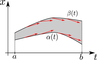
Figure 5: A funnel for the ODE $x^{\prime}=h(t,x)$. The red arrows indicate the vector field defined by $h$ and the gray area defines a funnel. Any solution which starts inside the funnel will stay there until $t=b$.

Proposition 28

Let $\alpha,\beta:I=[a,b)\subseteq\mathbb{R}\rightarrow\mathbb{R}$, where $b$ might be infinite, be a lower and upper fence, respectively, which define a funnel for the ODE $x^{\prime}=h(t,y)$, where $h$ is $C^{1}$. Assume also that $h$ satisfies a Lipschitz condition on the funnel. Then any solution which starts in the funnel at $t=a$ remains in the funnel for all $t\in[a,b)$.

Lemma 29

Let (2) define a structurally stable system over the compact set $\mathbb{D}\subseteq\mathbb{R}^{2}$. Then there exists $\varepsilon>0$ with the following properties. Let $x_{0}$ be an hyperbolic saddle point and let $\Omega_{1}(x_{0}),\Omega_{2}(x_{0})$ be defined as in Lemma 10. Let also $U_{x_{0}}$ be a local unstable manifold of $x_{0}$. Then $B(x_{0},\varepsilon)\subseteq\mathbb{D}$ and any trajectory starting in $B(x_{0},\varepsilon)$ will either: (i) converge to $x_{0}$ or (ii) converge to one of the attractors $\Omega_{1}(x_{0}),\Omega_{2}(x_{0})$.

Proof. Let $x_{0}$ be some saddle point of (2). First let us pick some $\varepsilon^{\ast}>0$ small enough so that $B(x_{0},\varepsilon^{\ast})\subseteq\mathbb{D}$. This is always possible since $x_{0}$ cannot be at the boundary of $\mathbb{D}$ or otherwise the system defined by (2) would not be structurally  stable. Moreover, by Peixoto’s theorem, the number of saddle points is finite and thus we can take $\varepsilon^{\ast}>0$ to be the minimum of all $\varepsilon^{\ast}$ for each saddle points. Since $d(x_{0},\partial\mathbb{D})>0$ it suffices to pick some $\varepsilon^{\ast}>0$ satisfying $\varepsilon^{\ast}<d(x_{0},\partial\mathbb{D})$ for all saddle points $x_{0}$. We also know that, by the Hartman-Grobman theorem, there is a homeomorphism $H$ from an open $U\subseteq\mathbb{D}$ containing $x_{0}$ to an open subset $V\subseteq\mathbb{R}^{2}$ containing the origin such that it maps trajectories of (2) in $U$ to trajectories of the following linearized ODE

$$x^{\prime}=A_{0}x$$ (28)

where $A_{0}=Df(x_{0})$ and $H(x_{0})=0$. Let us also suppose without loss of generality that $\varepsilon^{\ast}$ is small enough so that $B(x_{0},\varepsilon^{\ast})\subseteq U.$

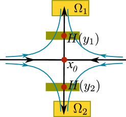
Figure 6: Flow near a saddle point, converging to two attractors $\Omega_{1}$ and $\Omega_{2}$.

Let $\Gamma_{1},\Gamma_{2}$ be defined as in the proof of Lemma 10 (i.e. they form, together with the point $x_{0}$, a local unstable manifold of $x_{0}$). Let $y_{1}\in\Gamma_{1}\cap B(x_{0},\varepsilon^{\ast})$. Then the trajectory $\phi_{t}(y_{1})$ will converge to some attractor $\Omega_{1}(x_{0})$. This means that the trajectory starting on $y_{1}$ will eventually reach a basin of attraction $\mathcal{B}_{\Omega_{1}(x_{0})}$ of the atractor $\Omega_{1}(x_{0})$ as defined in Lemma 26 in some time $T_{1}$ and then stay there, i.e. $\phi_{t}(y_{1})\in\mathcal{B}_{\Omega_{1}(x_{0})}$ for all $t\geq T_{1}$. Since $\mathcal{B}_{\Omega_{1}(x_{0})}$ is open, and due to Lemma 10, there is some $\delta_{1}>0$ such that $B(\phi_{t}(y_{1}),\delta_{1})\subseteq\mathcal{B}_{\Omega_{1}(x_{0})}$ for all $t\geq T_{1}$. Because the operator $\phi_{T_{1}}$ is continuous (Corollary 15) and because $B(\phi_{t}(y_{1}),\delta_{1})$ is an open set, this implies that

$$\phi_{T_{1}}^{-1}(B(\phi_{T_{1}}(y_{1}),\delta_{1}))=\phi_{-T_{1}}(B(\phi_{T_{1}}(y_{1}),\delta_{1}))$$

is an open neighborhood of $y_{1}$ with the property that any trajectory starting in this neighborhood will have reached the basin of attraction $\mathcal{B}_{\Omega_{1}(x_{0})}$ in time $T_{1}.$

By the Hartman-Grobman theorem, $H\circ\phi_{-T_{1}}(B(\phi_{T_{1}}(y_{1}),\delta_{1}))$ will be a neighborhood of $H(y_{1})$ for $\delta_{1}$ small enough. Moreover, $H(y_{1})$ will also belong to the unstable manifold of the origin in the linearized system (28). Similarly, we can pick a point $y_{2}\in\Gamma_{2}\cap B(x_{0},\varepsilon^{\ast})$ and $\delta_{2},T_{2}>0$ such that $\phi_{-T_{2}}(B(\phi_{T_{2}}(y_{2}),\delta_{2}))$ is an open neighborhood of $y_{2}$ with the property that any trajectory starting in this neighborhood will have reached the basin of attraction $\mathcal{B}_{\Omega_{2}(x_{0})}$ in time $T_{2}$. Furthermore, $H\circ\phi_{-T_{2}}(B(\phi_{T_{2}}(y_{2}),\delta_{2}))$ will be a neighborhood of $H(y_{2})$, and $H(y_{2})$ will also belong to the unstable manifold of the origin in the linearized system (28).

The classical theory of ODE gives us a way of finding the solutions of (28) explictly. Namely, since $x_{0}$ is an hyperbolic saddle point, $Df(x_{0})$ will have two eigenvalues $\lambda_{1}<0$ and $\lambda_{2}>0$. By picking appropriate coordinates (namely by picking as a basis for the coordinate system non-zero eigenvectors $v_{1},v_{2}$ associated to the eigenvalues $\lambda_{1},\lambda_{2}$, respectively. Without loss of generality this change of coordinates can be assumed to be comprised in the homeomorphism $H$), we see that this system is given by

$$\left[\begin{array}[c]{c}x_{1}^{\prime}\\ x_{2}^{\prime}\end{array}\right]=\left[\begin{array}[c]{cc}\lambda_{1}&0\\ 0&\lambda_{2}\end{array}\right]\left[\begin{array}[c]{c}x_{1}\\ x_{2}\end{array}\right]=\left[\begin{array}[c]{c}\lambda_{1}x_{1}\\ \lambda_{2}x_{2}\end{array}\right]$$ (29)

which has as solution curves (assuming that they start at $(x_{1}(0),x_{2}(0))$)

$$\left\{\begin{array}[c]{c}x_{1}=x_{1}(0)e^{\lambda_{1}t}\\ x_{2}=x_{2}(0)e^{\lambda_{2}t}\end{array}\right.$$ (30)

Graphically the flow is as depicted in Fig. 6. Without loss of generality, we assume that the homeomorphism $H$ maps the trajectories of (2) around $x_{0}$ to trajectories of (29) around the origin. Let $\delta>0$ be such that $B(H(y_{i}),\delta)\subseteq H\circ\phi_{-T_{i}}(B(\phi_{T_{i}}(y_{i}),\delta_{i}))$ for $i=1,2.$ From the expression of the solution (30) for the ODE (29), we conclude that any trajectory of (30) starting on a point $z=(z_{1},z_{2})\in B(0,\delta)$ will either: (i) converge to the origin (when $z_{2}=0$, i.e. when $z$ lies on the stable manifold) or (ii) enter the ball $B(H(y_{1}),\delta)$ (when $z_{2}>0$) or (iii) enter the ball $B(H(y_{2}),\delta)$ (when $z_{2}<0$). This implies that any trajectory starting on $H^{-1}(B(0,\delta))$ will either converge to $x_{0}$ or enter the open set $\cup_{i=1,2}\phi_{-T_{i}}(B(\phi_{T_{i}}(y_{i}),\delta_{i}))$. But since once a trajectory enters $\phi_{-T_{i}}(B(\phi_{T_{i}}(y_{i}),\delta_{i}))$ it will reach the basin of attraction $\mathcal{B}_{\Omega_{i}(x_{0})}$, we conclude the desired result for this case.   

Proof of Theorem 11. By Lemma 29, and the arguments used in its proof, we know that there is some $\lambda>0$ (independent of $i)$ such that any trajectory starting in $B(x_{i},\lambda)$ will either converge to $x_{i}$ (if the trajectory starts on the stable manifold of $x_{i}$) without leaving $B(x_{i},\lambda)$ or it will converge to some attractor $\Omega_{i}$.

Since there are no saddle connections on structurally stable systems $W^{u}(x_{i})$ cannot intersect $W^{s}(x_{j})$. Let

$$\delta=\min_{\begin{subarray}{c}i,j\in\{1,\ldots,n\}\\ i\neq j\end{subarray}}d(\overline{W^{u}(x_{i})},x_{j})>0.$$

Note also that the time it takes to go from a point $y_{i}\in W^{u}(x_{i})\cap\partial B(x_{i},\lambda)=\{y_{i},z_{i}\}$ to $\mathcal{B}_{\Omega_{i}}$ is finite. Moreover, because $\mathcal{B}_{\Omega}$ is open, we conclude that there is some $\epsilon>0$ such that $B(\phi_{t}(y_{i}),\epsilon)\subseteq\mathcal{B}_{\Omega_{i}}$. Hence, by Lemma 14, Corollary 15, and using techniques similar to those used in the proof of Lemma 29, we conclude that there is some $\delta^{\ast}>0$ and some $T^{\ast}\geq 0$, independent of $i$ and of $\{y_{i},z_{i}\}$, where $y_{i}$ and $z_{i}$ belong to “different sides” of $W^{u}(x_{i})\cap\partial B(x_{i},\lambda)$, such that any point in $B(w,\delta^{\ast}),$ $w\in\{y_{i},z_{i}\},$ will be on $\mathcal{B}_{\Omega}$ for some attractor $\Omega$ at time $T^{\ast}$ and, moreover, $d(\phi_{t}(B(w,\delta^{\ast})),\phi_{t}(w))<\delta/2$ for any $0\leq t\leq T^{\ast}.$ Since $d(\phi_{t}(w),x_{j})\geq\delta$ for all $0\leq t\leq T^{\ast}$, this implies that $d(\phi_{t}(B(w,\delta^{\ast})),x_{j})>\delta/2$. Therefore, it suffices to take $\varepsilon=\min(\delta^{\ast},\delta/2)$ to conclude that no trajectory leaving from $B(x_{i},\varepsilon)$ will enter $B(x_{j},\varepsilon)$ for $i\neq j.$

Appendix B Error bounds on the plane for Euler’s method

In this appendix we derive the error bound (6) for the Euler method used in Section 7.

We recall that in Euler’s method we start from a point $x_{0}$ and then obtain several iterates $x_{1},\ldots,x_{N}$ which approach the solution of the initial-value problem $z^{\prime}=f(z),$ $x(0)=x_{0}$ at times $0,h,\ldots,Nh\subseteq[0,b]$, where $b>0$, $h>0$ is the time step, and $x_{i}$ approximates $z(ih)$ for $i=1,\ldots,N$. Here we follow the arguments used in [1, pp. 346–350] for obtaining error bounds for the one-dimensional case to get error bounds for the two-dimensional case.

If $f=(f_{1},f_{2})$ and $z=(z_{1},z_{2})\in\mathbb{R}^{2}$, Taylor’s formula gives us

$$z_{1}(t_{0}+h)=z_{1}(t_{0})+hz_{1}^{\prime}(t_{0})+\frac{h^{2}}{2}z_{1}^{\prime\prime}(\xi)$$

for some $t_{0}<\xi<t$. Note that $z_{1}^{\prime}(\xi)=f_{1}(z(\xi))=f(z_{1}(\xi),z_{2}(\xi))$. Hence

$$z_{1}^{\prime\prime}(\xi) =\frac{\partial f_{1}}{\partial z_{1}}(z(\xi))z_{1}^{\prime}(\xi)+\frac{\partial f_{1}}{\partial z_{2}}(z(\xi))z_{2}^{\prime}(\xi)$$

$$=\frac{\partial f_{1}}{\partial z_{1}}(z(\xi))f_{1}(z(\xi))+\frac{\partial f_{1}}{\partial z_{2}}(z(\xi))f_{2}(z(\xi)).$$

If we take $M=\max_{x\in\mathbb{D}}(\left\|f(x)\right\|,\left\|Df(x)\right\|)$, then we get

$$\left\|z_{1}^{\prime\prime}(\xi)\right\|\leq 2M^{2}.$$

A similar bound holds for $\left\|z_{2}^{\prime\prime}(\xi)\right\|$. Let us now assume that the rounding error is bounded by $\rho>0$ when using Euler’s method (4) and take $X_{i}=z(hi)$ for $i=0,1,\ldots,N$. Then

$$X_{i+1} =X_{i}+hf(X_{i})+\frac{h^{2}}{2}(z_{1}^{\prime\prime}(\xi_{i,1}),z_{1}^{\prime\prime}(\xi_{i,2}))$$

$$x_{i+1} =x_{i}+hf(x_{i})+\rho_{i}$$

where $\rho_{i}$ is the rounding error on each step, with $\left|\rho_{i}\right|\leq\rho$ and $i=1,\ldots,N$. Subtracting both equations, we get

$$e_{i+1}=e_{i}+h\left(f(X_{i})-f(x_{i})\right)+\frac{h^{2}}{2}(z_{1}^{\prime\prime}(\xi_{i,1}),z_{1}^{\prime\prime}(\xi_{i,2}))-\rho_{i}$$

where $e_{i}=X_{i}-x_{i}$. Let $\tau_{i}=\frac{h}{2}(z_{1}^{\prime\prime}(\xi_{i,1}),z_{1}^{\prime\prime}(\xi_{i,2}))-\frac{\rho_{i}}{h}$. Then the above identity yields (note that since $M\geq\left\|Df(x)\right\|$ on $\mathbb{D}$, it works as a Lipschitz constant there, but let us just consider a Lipschitz constant $L>0$ there)

$$\left\|e_{i+1}\right\| \leq\left\|e_{i}\right\|+h\left(L\left\|e_{i}\right\|\right)+h\left\|\tau_{i}\right\|$$

$$\leq(1+hL)\left\|e_{i}\right\|+h\left\|\tau_{i}\right\|$$

Applying this last formula recursively, we get

$$\left\|e_{i}\right\| \leq(1+hL)^{i}\left\|e_{0}\right\|+\left(1+(1+hL)+\ldots+(1+hL)^{i-1}\right)h\left\|\tau_{i}\right\|$$

$$\leq(1+hL)^{i}\left\|e_{0}\right\|+\left(1+(1+hL)+\ldots+(1+hL)^{i-1}\right)h\tau$$

where $\tau=hM^{2}+\rho/h$. Using the formula for the sum of a finite geometric series $(r\neq 1)$

$$1+r+r^{2}+\ldots+r^{n-1}=\frac{r^{n}-1}{r-1}$$

we get

$$\left\|e_{i}\right\|\leq(1+hL)^{i}\left\|e_{0}\right\|+\left(\frac{(1+hL)^{i}-1}{L}\right)\tau.$$

Since

$$(1+hL)^{i}\leq e^{ihL}\leq e^{bL}$$

The last inequality then yields

$$\left\|e_{i}\right\|\leq e^{bL}\left\|e_{0}\right\|+\left(\frac{e^{bL}-1}{L}\right)\left(hM^{2}+\frac{\rho}{h}\right)$$

which is essentially (6).

References

- [1] K. E. Atkinson. An Introduction to Numerical Analysis. John Wiley & Sons, 2nd edition, 1989.
- [2] S. Banach and S. Mazur. Sur les fonctions calculables. Ann. Soc. Pol. de Math., 16, 1937.
- [3] G. Birkhoff and G.-C. Rota. Ordinary Differential Equations. John Wiley & Sons, 4th edition, 1989.
- [4] O. Bournez, D. S. Graça, and A. Pouly. On the complexity of solving initial value problems. In Proc. 37h International Symposium on Symbolic and Algebraic Computation (ISSAC 2012), pages 115–121. Association for Computing Machinery, 2012.
- [5] V. Brattka, P. Hertling, and K. Weihrauch. A tutorial on computable analysis. In S. B. Cooper, B. Löwe, and A. Sorbi, editors, New Computational Paradigms: Changing Conceptions of What is Computable, pages 425–491. Springer, 2008.
- [6] M. Braverman. Computational complexity of euclidean sets: hyperbolic Julia sets are poly-time computable. In V. Brattka, L. Staiger, and K. Weihrauch, editors, Proc. 6th Workshop on Computability and Complexity in Analysis (CCA 2004), volume 120 of Electronic Notes in Theoretical Computer Science, pages 17–30. Elsevier, 2005.
- [7] M. Braverman and M. Yampolsky. Non-computable Julia sets. Journal of the American Mathematical Society, 19(3):551–578, 2006.
- [8] M. Braverman and M. Yampolsky. Computability of Julia Sets. Springer, 2009.
- [9] P. Collins and D. S. Graça. Effective computability of solutions of ordinary differential equations the thousand monkeys approach. In V. Brattka, R. Dillhage, T. Grubba, and A. Klutsch, editors, Proc. 5th International Conference on Computability and Complexity in Analysis (CCA 2008), volume 221 of Electronic Notes in Theoretical Computer Science, pages 103–114. Elsevier, 2008.
- [10] P. Collins and D. S. Graça. Effective computability of solutions of differential inclusions — the ten thousand monkeys approach. Journal of Universal Computer Science, 15(6):1162–1185, 2009.
- [11] M. Dellnitz, G. Froyland, and O. Junge. Ergodic Theory, Analysis, and Efficient Simulation of Dynamical Systems, chapter The Algorithms Behind GAIO – Set Oriented Numerical Methods for Dynamical Systems, pages 145–174. Springer, 2001.
- [12] D. S. Graça, C. Rojas, and N. Zhong. Computing geometric Lorenz attractors with arbitrary precision. Transactions of the American Mathematical Society, 370:2955–2970, 2018.
- [13] D. S. Graça and N. Zhong. Computability of differential equations. In V. Brattka and P. Hertling, editors, Handbook of Computability and Complexity in Analysis, pages 71–99. Springer International Publishing, Cham, 2021.
- [14] D. S. Graça, N. Zhong, and J. Buescu. Computability, noncomputability and undecidability of maximal intervals of IVPs. Transactions of the American Mathematical Society, 361(6):2913–2927, 2009.
- [15] D. S. Graça, N. Zhong, and H. S. Dumas. The connection between computability of a nonlinear problem and its linearization: the Hartman-Grobman theorem revisited. Theoretical Computer Science, 457(26):101–110, 2012.
- [16] D. S. Graça and N. Zhong. The set of hyperbolic equilibria and of invertible zeros on the unit ball is computable. Theoretical Computer Science, 895:48–54, 2021.
- [17] J. Guckenheimer and P. Holmes. Nonlinear Oscillations, Dynamical Systems, and Bifurcation of Vector Fields. Springer, 1983.
- [18] J. H. Hubbard and B. H. West. Differential Equations: A Dynamical Systems Approach — Higher-Dimensional Systems. Springer, 1995.
- [19] Y. Ilyashenko. Centennial history of Hilbert’s 16th problem. Bulletin of the American Mathematical Society, 39:301–354, 2002.
- [20] A. Kawamura. Lipschitz continuous ordinary differential equations are polynomial-space complete. Computational Complexity, 19(2):305–332, 2010.
- [21] A. Kawamura, H. Ota, C. Rösnick, and M. Ziegler. Computational complexity of smooth differential equations. Logical Methods in Computer Science, 10(1:6):1–15, 2014.
- [22] K.-I Ko. Complexity Theory of Real Functions. Birkhäuser, 1991.
- [23] Y. Matiyasevich. Hilbert’s 10th Problem. The MIT Press, 1993.
- [24] S. Mazur. Computable Analysis, volume 63. Rosprawy Matematyczne, Warsaw, 1963.
- [25] W. Miller. Recursive function theory and numerical analysis. Journal of Computer and System Sciences, 4:465–472, 1970.
- [26] N. Müller and B. Moiske. Solving initial value problems in polynomial time. In Proc. 22 JAIIO - PANEL ’93, Part 2, pages 283–293, 1993.
- [27] N. Th. Müller. Uniform computational complexity of taylor series. In T. Ottmann, editor, Proc. 14th International Colloquium on Automata, Languages and Programming (ICALP 1987), volume 267 of Lecture Notes in Computer Science, pages 435–444. Springer, 1987.
- [28] J. R. Munkres. Topology. Pearson, 2nd edition, 2000.
- [29] P. Odifreddi. Classical Recursion Theory, volume 1. Elsevier, 1989.
- [30] M. Peixoto. On structural stability. Annals of Mathematics, 69(1):199–222, 1959.
- [31] M. Peixoto. Structural stability on two-dimensional manifolds. Topology, 1:101–121, 1962.
- [32] L. Perko. Differential Equations and Dynamical Systems. Springer, 3rd edition, 2001.
- [33] A. Pouly and D. S. Graça. Computational complexity of solving polynomial differential equations over unbounded domains. Theoretical Computer Science, 626(2):67–82, 2016.
- [34] M. B. Pour-El and J. I. Richards. Computability in Analysis and Physics. Springer, 1989.
- [35] R. Rettinger. A fast algorithm for Julia sets of hyperbolic rational functions. In V. Brattka, L. Staiger, and K. Weihrauch, editors, Proc. 6th Workshop on Computability and Complexity in Analysis (CCA 2004), volume 120 of Electronic Notes in Theoretical Computer Science, pages 145–157. Elsevier, 2005.
- [36] M. Sipser. Introduction to the Theory of Computation. Cengage Learning, 3rd edition, 2012.
- [37] W. Tucker. Computing accurate Poincaré maps. Physica D, 171:127–137, 2002.
- [38] A. M. Turing. On computable numbers, with an application to the entscheidungsproblem. Proceedings of the London Mathematical Society, s2-42(1):230–265, 1937.
- [39] K. Weihrauch. Computable Analysis: an Introduction. Springer, 2000.
- [40] K. Weihrauch and N. Zhong. Computable analysis of the abstract Cauchy problem in Banach spaces and its applications I. Mathematical Logic Quarterly, 53(4-5):511 – 531, 2007.
- [41] M. Ziegler and V. Brattka. Computability in linear algebra. Theoretical Computer Science, 326:187–211, 2004.