Second and fourth moments of the charge density and neutron-skin thickness of atomic nuclei

Abstract

A method is presented to extract the neutron-skin thickness of atomic nuclei from the second and fourth moments of the electric charge distribution. We show that the value of the proton fourth moment must be independently known in order to estimate the neutron skin thickness experimentally. To overcome this problem, we propose the use of a strong linear correlation among the second and fourth moments of the proton distribution as calculated with several energy density functionals of common use. We take special care in estimating the errors associated with the different contributions to the neutron radius and show, for the first time, the analytic expressions for the spin-orbit contribution to the charge fourth moments of neutrons and protons. To reduce the uncertainty on the extraction of the neutron radius, two neighboring even-even isotopes are used. Nevertheless, the error on the fourth moment of the proton distribution, even if determined or assumed with large accuracy, dominates and prevents the present method from being applied for a sound determination of the neutron skin thickness.

I Introduction

The study of the neutron-skin thickness $\Delta r_{np}=\sqrt{\left\langle{r^{2}}\right\rangle_{n}}-\sqrt{\left\langle{r^{2}}\right\rangle_{p}}$ of atomic nuclei has become one of the hottest topics in nuclear physics during the past decades Bender et al. (2003); Tsang et al. (2012); Lattimer (2012); Hebeler et al. (2015); Thiel et al. (2019). Here, $\left\langle{r^{2}}\right\rangle_{p}$ and $\left\langle{r^{2}}\right\rangle_{n}$ denote the second moments of the proton and neutron density distributions, $\rho_{p}$ and $\rho_{n}$, respectively. A precise determination of the neutron-skin thickness of a heavy nucleus sets a basic constraint on the nuclear symmetry energy, in particular, its density dependence around the saturation density Yoshida and Sagawa (2004, 2006); Roca-Maza et al. (2013); Viñas et al. (2014); Typel (2014); Pais et al. (2016); Mondal et al. (2016). For example, the neutron-skin thickness of ${}^{208}\mathrm{Pb}$ is known to be directly related to the slope parameter of the symmetry energy $L$ by $\Delta r_{np}\left({}^{208}\mathrm{Pb}\right)\left[\mathrm{fm}\right]=0.101(3)+0.001\,47(5)L\left[\mathrm{MeV}\right]$ ($r=0.98$) if one exploits the prediction by a large and representative set of modern nuclear energy density functionals (EDFs) Roca-Maza et al. (2011). The equation of state of nuclear matter, which provides the value of $L$, is also known to be related to a wide range of questions in nuclear physics and astrophysics Myers and Swiatecki (1980); Stringari (1983); Sagawa (2002); Chen et al. (2003); Baran et al. (2005); Li et al. (2008); Di Toro et al. (2010); Gandolfi et al. (2012); Colò et al. (2014); Hebeler et al. (2013); Malik et al. (2018); Horowitz (2019); Morfouace et al. (2019); Burrello et al. (2019); Tong et al. (2020). For more detail, see the review papers, e.g., Refs. Lattimer (2012); Viñas et al. (2014); Lattimer (2014); Baldo and Burgio (2016); Gandolfi et al. (2019). Yet, our knowledge of neutron-skin thickness is limited even in the stable nuclei, and neutron-skin thickness of the unstable nuclei has not been measured yet.

The parity-violating elastic electron scattering Roca-Maza et al. (2011); Donnelly (1990); Paschke et al. (2011); Armstrong and McKeown (2012); Horowitz et al. (2012); Abrahamyan et al. (2012); Souder and Paschke (2016); Adhikari et al. (2021) and the isotopic ratio of atomic parity violation Fortson et al. (1990) were suggested as clean and model-independent probes of neutron densities. However, measuring parity-violating asymmetries of the order of a part per $10^{6}$ is challenging. The present result is $\Delta r_{np}=0.283\pm 0.071\,\mathrm{fm}$ at the PREX-II experiment Paschke et al. (2011); Adhikari et al. (2021) for ${}^{208}\mathrm{Pb}$. The ambitious efforts in JLab aim at determining the $\Delta r_{np}$ of ${}^{48}\mathrm{Ca}$ with higher precisions as well Horowitz et al. (2014).

The hadronic probes, including polarized-proton scattering Zenihiro et al. (2010); Sakaguchi and Zenihiro (2017), $\alpha$ scattering Tatischeff et al. (1972), anti-protonic atoms Alex Brown et al. (2007), $\pi^{\pm}$ scattering Johnson et al. (1979); Barnett et al. (1985), and anti-proton scattering Lenske and Kienle (2007); Makiguchi et al. (2020), as well as the nuclear excitations, such as isovector resonances Krasznahorkay et al. (1999), have been also widely used or proposed to determine the neutron-skin thickness and cover a large area of the nuclear chart. Nevertheless, even if some of these experiments reach small errors, all hadronic probes require model assumptions to deal with the strong force, which, in principle, introduces systematic uncertainties.

In contrast, the study of the charge density distribution $\rho_{\scriptstyle{\text{{{{ch}}}}}}$ of atomic nuclei, which is essentially dominated by the proton density distribution $\rho_{p}$, can be experimentally determined with no model dependence via elastic electron scattering Lyman et al. (1951); Hofstadter et al. (1953a); Pidd et al. (1953); Hofstadter et al. (1953b, 1954); Hofstadter (1956). The $\rho_{\scriptstyle{\text{{{{ch}}}}}}$ of many stable nuclei has been measured with very high accuracy De Vries et al. (1987). As a big step further, the electron scattering of unstable nuclei is foreseen in the near future, for instance, in the SCRIT facility in RIKEN Wakasugi et al. (2013, 2004); Tsukada et al. (2017) and in the ELISe facility in FAIR Antonov et al. (2011); Berg et al. (2011). Nowadays, essentially the only way to provide the information of the charge radii of unstable nuclei is the laser spectroscopy of atoms. The laser spectroscopy of atoms was established in the late 1910s Aronberg (1918); Merton (1920) and has been applied to long-lived unstable nuclei since the 1960s Marrus and McColm (1965); Hühnermann and Wagner (1966); Jacquinot and Klapisch (1979); Kluge and Nörtershäuser (2003); Campbell et al. (2016); Flambaum and Dzuba (2019). The charge radii of nuclei located on wide region of the nuclear chart have been measured Angeli and Marinova (2013), and are still being measured at many radioactive isotope beam facilities.

Recently, the fourth moment of the charge distribution has been highlighted as a possible proxy to access information of the neutron root-mean-square radius Kurasawa and Suzuki (2019); Reinhard et al. (2020); Kurasawa et al. (2021). Kurasawa and Suzuki Kurasawa and Suzuki (2019) suggested that the fourth moment of the charge density distribution $\left\langle{r^{4}}\right\rangle_{\scriptstyle{\text{{{{ch}}}}}}$, which can be measured by the electron scattering Kurasawa et al. (2021) or the laser spectroscopy Papoulia et al. (2016), includes the information of the neutron radius and thus the neutron-skin thickness. This is because the neutron distributions $\rho_{n}$ of atomic nuclei do contribute to their charge density distributions $\rho_{\scriptstyle{\text{{{{ch}}}}}}$ Bertozzi et al. (1972); Kurasawa and Suzuki (2000); Naito et al. (2020) since a neutron has a finite size and has a corresponding internal charge distribution, which is usually encoded in the electromagnetic form factor of the neutron. In other words, precise measurements of $\rho_{\scriptstyle{\text{{{{ch}}}}}}$ may be able to provide information on $\rho_{n}$ as well as $\rho_{p}$ and, thus, determine the neutron-skin thickness $\Delta r_{np}$. For instance, Ref. Kurasawa et al. (2021) showed the feasibility to extract $\left\langle{r^{2}}\right\rangle_{n}$ using $\left\langle{r^{2}}\right\rangle_{\scriptstyle{\text{{{{ch}}}}}}$ and $\left\langle{r^{4}}\right\rangle_{\scriptstyle{\text{{{{ch}}}}}}$ for ${}^{40}\mathrm{Ca}$, ${}^{48}\mathrm{Ca}$, and ${}^{208}\mathrm{Pb}$ isotopes by using the linear correlations among second and fourth moments of proton, neutron, and charge density distributions, and eventually, the uncertainty of $\left\langle{r^{2}}\right\rangle_{n}$ is quite small. Indeed, this relied on a correlation for these specific nuclei based on a specific type of models, and, hence, it is questionable whether that method can be applied, in general.

To answer this question, in this paper, we discuss the feasibility of extracting $\left\langle{r^{2}}\right\rangle_{n}$ from the second and fourth moments of the charge density distribution $\left\langle{r^{2}}\right\rangle_{\scriptstyle{\text{{{{ch}}}}}}$ and $\left\langle{r^{4}}\right\rangle_{\scriptstyle{\text{{{{ch}}}}}}$, applying the general modeling of electromagnetic form factors of both protons and neutrons avoiding as much as possible the use of model-induced correlations. We also explore a method to extract the neutron-skin thickness by employing the information of $\rho_{\scriptstyle{\text{{{{ch}}}}}}$ of two neighboring even-even isotopes to cancel large part of the spin-orbit contributions to $\left\langle{r^{2}}\right\rangle_{\scriptstyle{\text{{{{ch}}}}}}$ and $\left\langle{r^{4}}\right\rangle_{\scriptstyle{\text{{{{ch}}}}}}$ and reduce the uncertainty due to the nucleon form factors and the pairing correlation. To extract $\left\langle{r^{2}}\right\rangle_{n}$ from $\left\langle{r^{2}}\right\rangle_{\scriptstyle{\text{{{{ch}}}}}}$ and $\left\langle{r^{4}}\right\rangle_{\scriptstyle{\text{{{{ch}}}}}}$, we will show that the key issue is how to accurately determine $\left\langle{r^{4}}\right\rangle_{p}$.

This paper is organized as follows: First, the general equations for $\left\langle{r^{2}}\right\rangle_{\scriptstyle{\text{{{{ch}}}}}}$ and $\left\langle{r^{4}}\right\rangle_{\scriptstyle{\text{{{{ch}}}}}}$ will be given in Sec. II as functions of the second and fourth moments of the neutron and proton density distributions and of the parameters defining the neutron and proton electric form factors. Second, a novel equation will be introduced in Sec. III to reduce the uncertainty due to the magnetic contribution and nucleon form factors. In this equation, two neighboring even-even nuclei are used in which the same single-particle orbitals are being filled and, thus, the uncertainties associated with the latter effects are expected to be reduced. Third, the possibility to derive theoretically the fourth moment of the proton distribution $\left\langle{r^{4}}\right\rangle_{p}$ will be discussed in Sec. IV.1. Then, we will show the benchmark calculation of the novel method in Sec. IV.2. We will also show the uncertainty due to the nucleon form factors in Sec. IV.3. Finally, the conclusion and perspectives will be given in Sec. V.

II Second and Fourth Moments of Charge Distribution

First, we would recall the relationship between $\left\langle{r^{n}}\right\rangle_{\scriptstyle{\text{{{{ch}}}}}}$ and $\left\langle{r^{n}}\right\rangle_{\tau}$, which is originally derived in Refs. Kurasawa and Suzuki (2019); Reinhard and Nazarewicz (2021). It is convenient to consider the finite-size effects of nucleons on the charge density distribution in the momentum space, i.e.,

$$\tilde{\rho}_{\scriptstyle{\text{{{{ch}}}}}}\left(q\right)=\sum_{\tau=p,\,n}\left[\tilde{G}_{\scriptstyle{\text{{{{E}}}}}\tau}\left(q^{2}\right)\tilde{\rho}_{\tau}\left(q\right)+\frac{\tilde{G}_{\scriptstyle{\text{{{{M}}}}}\tau}\left(q^{2}\right)-\tilde{G}_{\scriptstyle{\text{{{{E}}}}}\tau}\left(q^{2}\right)}{1+q^{2}/4M_{\tau}^{2}}\left(\frac{q^{2}}{4M_{\tau}^{2}}\tilde{\rho}_{\tau}\left(q\right)+\frac{q}{2M_{\tau}}\tilde{F}_{\scriptstyle{\text{{{{T}}}}}\tau}\left(q\right)\right)\right],$$ (1)

where $M_{\tau}$ is the nucleon mass Zyla et al. (2020), $\tilde{G}_{\scriptstyle{\text{{{{E}}}}}\tau}$ and $\tilde{G}_{\scriptstyle{\text{{{{M}}}}}\tau}$ are the electric and magnetic form factors of nucleons, $\rho_{\scriptstyle{\text{{{{ch}}}}}}$, $\rho_{p}$, and $\rho_{n}$, respectively, are the charge, proton, and neutron density distributions, which are assumed to have spherical symmetry in this paper, $\tilde{\rho}$ is the Fourier transform of the density $\rho$, and $\tilde{F}_{\scriptstyle{\text{{{{T}}}}}\tau}$ is the tensor form factor, whose definition is given in Eq. (34b). Note that $\tilde{\rho}_{\scriptstyle{\text{{{{ch}}}}}}$ is sometimes called the (charge) form factor of the nucleus. The Fourier transform is defined by

$$\tilde{\rho}_{\tau}\left(q\right)=\int\rho_{\tau}\left(r\right)\,e^{-i{\bm{q}}\cdot{\bm{r}}}\,d{\bm{r}}=4\pi\int_{0}^{\infty}\rho_{\tau}\left(r\right)\,\frac{\sin\left(qr\right)}{qr}r^{2}\,dr.$$ (2)

The $2n$th moment of $\rho_{\tau}$ is defined by

$$\left\langle{r^{2n}}\right\rangle_{\tau}=\frac{\int\rho_{\tau}\left({\bm{r}}\right)r^{2n}\,d{\bm{r}}}{\int\rho_{\tau}\left({\bm{r}}\right)\,d{\bm{r}}}.$$ (3)

In particular, with the assumption of spherical symmetry, this expression for $\rho_{\scriptstyle{\text{{{{ch}}}}}}$ can be simplified into 

$$\left\langle{r^{2n}}\right\rangle_{\scriptstyle{\text{{{{ch}}}}}}=\frac{\left(-1\right)^{n}4\pi}{Z}\sum_{\tau=p,\,n}\int_{0}^{\infty}\left\{\frac{1}{q}\frac{d^{2n}}{dq^{2n}}\tilde{G}_{\scriptstyle{\text{{{{E}}}}}\tau}\left(q^{2}\right)\,\sin\left(qr\right)\right\}_{q=0}\rho_{\tau}\left(r\right)\,r\,dr,$$ (4)

where derivation of this equation is shown in Appendix A. Using Eq. (4), the second and fourth moments of $\rho_{\scriptstyle{\text{{{{ch}}}}}}$ read

$$\left\langle{r^{2}}\right\rangle_{\scriptstyle{\text{{{{ch}}}}}} =\left\langle{r^{2}}\right\rangle_{p}+\left(r_{\scriptstyle{\text{{{{E}}}}}p}^{2}+\frac{N}{Z}r_{\scriptstyle{\text{{{{E}}}}}n}^{2}\right)+\left\langle{r^{2}}\right\rangle_{\scriptstyle{\text{{{{SO}}}}}p}+\frac{N}{Z}\left\langle{r^{2}}\right\rangle_{\scriptstyle{\text{{{{SO}}}}}n},$$ (5a)

$$\left\langle{r^{4}}\right\rangle_{\scriptstyle{\text{{{{ch}}}}}} =\left\langle{r^{4}}\right\rangle_{p}+\frac{10}{3}\left(r_{\scriptstyle{\text{{{{E}}}}}p}^{2}\left\langle{r^{2}}\right\rangle_{p}+\frac{N}{Z}r_{\scriptstyle{\text{{{{E}}}}}n}^{2}\left\langle{r^{2}}\right\rangle_{n}\right)+\left(r_{\scriptstyle{\text{{{{E}}}}}p}^{4}+\frac{N}{Z}r_{\scriptstyle{\text{{{{E}}}}}n}^{4}\right)+\left\langle{r^{4}}\right\rangle_{\scriptstyle{\text{{{{SO}}}}}p}+\frac{N}{Z}\left\langle{r^{4}}\right\rangle_{\scriptstyle{\text{{{{SO}}}}}n},$$ (5b)

where $r_{\scriptstyle{\text{{{{E}}}}}\tau}^{2}$ and $r_{\scriptstyle{\text{{{{E}}}}}\tau}^{4}$ are the second and fourth moments of charge distribution of the nucleon $\tau$, respectively [note that $r_{\scriptstyle{\text{{{{E}}}}}\tau}^{4}\neq\left(r_{\scriptstyle{\text{{{{E}}}}}\tau}^{2}\right)^{2}$]. For a detailed derivation, see Appendix B. Here, $\left\langle{r^{n}}\right\rangle_{\scriptstyle{\text{{{{SO}}}}}\tau}$ is called the spin-orbit contribution due to the existence of the magnetic form factor, and if one considers only the first term of Eq. (1), it vanishes. The spin-orbit contributions $\left\langle{r^{n}}\right\rangle_{\scriptstyle{\text{{{{SO}}}}}\tau}$ read

$$\left\langle{r^{2}}\right\rangle_{\scriptstyle{\text{{{{SO}}}}}\tau} \simeq\frac{\kappa_{\tau}}{M_{\tau}^{2}N_{\tau}}\sum_{a\in\scriptstyle{\text{{{{occ}}}}}}{\mathcal{N}}_{a\tau}\left\langle{{\bm{l}}\cdot{\bm{\sigma}}}\right\rangle,$$ (6a)

$$\left\langle{r^{4}}\right\rangle_{\scriptstyle{\text{{{{SO}}}}}\tau} \simeq\frac{10}{M_{\tau}^{2}N_{\tau}}\sum_{a\in\scriptstyle{\text{{{{occ}}}}}}\left[\frac{\kappa_{\tau}}{5}\left\langle{r^{2}}\right\rangle_{g_{a\tau}}+\frac{r_{\scriptstyle{\text{{{{M}}}}}\tau}^{2}-r_{\scriptstyle{\text{{{{E}}}}}\tau}^{2}}{3}+\frac{\kappa_{\tau}}{2M_{\tau}^{2}}\right]{\mathcal{N}}_{a\tau}\left\langle{{\bm{l}}\cdot{\bm{\sigma}}}\right\rangle,$$ (6b)

where $N_{\tau}=Z$ for proton ($\tau=p$) or charge distribution and $N_{\tau}=N$ for neutron ($\tau=n$) distribution, $\kappa_{\tau}$ is the anomalous magnetic moment of the nucleon $\tau$ Zyla et al. (2020), and $r_{\scriptstyle{\text{{{{M}}}}}\tau}^{2}$ is the second moment of magnetic distribution of the nucleon $\tau$. The index $a=\left(n,\kappa,m\right)$ is the set of the quantum numbers of a single-particle orbital, whose occupation number is ${\mathcal{N}}_{a\tau}$, and $\left\langle{r^{2}}\right\rangle_{g_{a\tau}}$ is the second moment of the radial part of the upper component of single-particle Dirac spinor $g_{a\tau}\left(r\right)$, which is approximately identical to the radial part of a single-particle orbital in the nonrelativistic scheme. Detailed derivations are shown in Appendices A and B, and see also Ref. Horowitz and Piekarewicz (2012) for Eq. (6a).

One can simply assume that $\left\langle{r^{2}}\right\rangle_{g_{a\tau}}\simeq\left\langle{r^{2}}\right\rangle_{\tau}$, which is probably a good approximation except in weakly bound systems, and estimate the spin-orbit contribution $\left\langle{r^{2}}\right\rangle_{\scriptstyle{\text{{{{SO}}}}}\tau}$ and $\left\langle{r^{4}}\right\rangle_{\scriptstyle{\text{{{{SO}}}}}\tau}$ based on the naive shell-model occupancies. The approximation brings us to

$$\left\langle{r^{4}}\right\rangle_{\scriptstyle{\text{{{{SO}}}}}\tau}\simeq\frac{10}{M_{\tau}^{2}N_{\tau}}\left[\frac{\kappa_{\tau}}{5}\left\langle{r^{2}}\right\rangle_{\tau}+\frac{r_{\scriptstyle{\text{{{{M}}}}}\tau}^{2}-r_{\scriptstyle{\text{{{{E}}}}}\tau}^{2}}{3}+\frac{\kappa_{\tau}}{2M_{\tau}^{2}}\right]\sum_{a\in\scriptstyle{\text{{{{occ}}}}}}{\mathcal{N}}_{a\tau}\left\langle{{\bm{l}}\cdot{\bm{\sigma}}}\right\rangle$$ (7)

and we will discuss below the role of the occupancies ${\mathcal{N}}_{a\tau}$ (cf. Sec. IV).

In this paper, we use the electric form factors of protons and neutrons $\tilde{G}_{\scriptstyle{\text{{{{E}}}}}\tau}$ proposed in Ref. Alberico et al. (2009) in which values of $r_{\scriptstyle{\text{{{{E}}}}}\tau}^{2}$, $r_{\scriptstyle{\text{{{{E}}}}}\tau}^{4}$, and $r_{\scriptstyle{\text{{{{M}}}}}\tau}^{2}$ are

$$r_{\scriptstyle{\text{{{{E}}}}}\tau}^{2} =\begin{cases}0.75036\,\mathrm{fm}^{2}&\text{(Proton)},\\ -0.11146\,\mathrm{fm}^{2}&\text{(Neutron)},\end{cases}$$ (8a)

$$r_{\scriptstyle{\text{{{{E}}}}}\tau}^{4} =\begin{cases}1.6228\,\mathrm{fm}^{4}&\text{(Proton)},\\ -0.33398\,\mathrm{fm}^{4}&\text{(Neutron)},\end{cases}$$ (8b)

$$r_{\scriptstyle{\text{{{{M}}}}}\tau}^{2} =\begin{cases}0.74439\,\mathrm{fm}^{2}&\text{(Proton)},\\ 0.86381\,\mathrm{fm}^{2}&\text{(Neutron)},\end{cases}$$ (8c)

respectively. Note that these values of $r_{\scriptstyle{\text{{{{E}}}}}\tau}^{2}$ and $r_{\scriptstyle{\text{{{{M}}}}}\tau}^{2}$ are accurate enough for our purpose Zyla et al. (2020) and some form factors available in the literature Friedrich and Walcher (2003) give the opposite sign for $r_{\scriptstyle{\text{{{{E}}}}}n}^{4}$, but this difference does not change the discussion presented in this paper.

III Isotope-shift Method

We then consider whether $\left\langle{r^{2}}\right\rangle_{n}$ can be extracted from experimental data of $\left\langle{r^{2}}\right\rangle_{\scriptstyle{\text{{{{ch}}}}}}$ and $\left\langle{r^{4}}\right\rangle_{\scriptstyle{\text{{{{ch}}}}}}$ provided by the electron scattering experiments or isotope shift by using Eqs. (5a) and (5b). Although $\left\langle{r^{2}}\right\rangle_{\scriptstyle{\text{{{{SO}}}}}\tau}$ and $\left\langle{r^{4}}\right\rangle_{\scriptstyle{\text{{{{SO}}}}}\tau}$ are derived in Eqs. (6a) and (7), several approximations have been introduced to derive them, as shown in Appendix B. To reduce uncertainties introduced by such approximations and by the nucleon form factors, we will consider two isotopes with the neutron numbers $N-2$ and $N$, instead of only one nucleus. Since $\left\langle{r^{2}}\right\rangle_{\scriptstyle{\text{{{{SO}}}}}\tau}$ and $\left\langle{r^{4}}\right\rangle_{\scriptstyle{\text{{{{SO}}}}}\tau}$ are written as the sum of $\left\langle{{\bm{l}}\cdot{\bm{\sigma}}}\right\rangle$ over all the single-particle orbitals, $\left\langle{r^{n}}\right\rangle_{\scriptstyle{\text{{{{SO}}}}}\tau}$ for two isotopes in the same neutron shell are almost the same. Hence, a large cancellation of such uncertainty can be expected.

Comparing Eq. (5b) for two isotopes with their neutron numbers $N-2$ and $N$, the master equation,

$$\left\langle{r^{2}}\right\rangle_{n}^{\left(N-2\right)}$$

$$= \,\frac{3}{10}\frac{Z}{r_{\scriptstyle{\text{{{{E}}}}}n}^{2}}\left[\frac{\left\langle{r^{4}}\right\rangle_{\scriptstyle{\text{{{{ch}}}}}}^{\left(N\right)}-\left\langle{r^{4}}\right\rangle_{\scriptstyle{\text{{{{ch}}}}}}^{\left(N-2\right)}}{2}-\frac{\left\langle{r^{4}}\right\rangle_{p}^{\left(N\right)}-\left\langle{r^{4}}\right\rangle_{p}^{\left(N-2\right)}}{2}-\frac{\left\langle{r^{4}}\right\rangle_{\scriptstyle{\text{{{{SO}}}}}p}^{\left(N\right)}-\left\langle{r^{4}}\right\rangle_{\scriptstyle{\text{{{{SO}}}}}p}^{\left(N-2\right)}}{2}\right]-Z\frac{r_{\scriptstyle{\text{{{{E}}}}}p}^{2}}{r_{\scriptstyle{\text{{{{E}}}}}n}^{2}}\frac{\left\langle{r^{2}}\right\rangle_{\scriptstyle{\text{{{{ch}}}}}}^{\left(N\right)}-\left\langle{r^{2}}\right\rangle_{\scriptstyle{\text{{{{ch}}}}}}^{\left(N-2\right)}}{2}$$

$$\,-N\frac{\left\langle{r^{2}}\right\rangle_{n}^{\left(N\right)}-\left\langle{r^{2}}\right\rangle_{n}^{\left(N-2\right)}}{2}-\frac{3}{10}\frac{N}{r_{\scriptstyle{\text{{{{E}}}}}n}^{2}}\frac{\left\langle{r^{4}}\right\rangle_{\scriptstyle{\text{{{{SO}}}}}n}^{\left(N\right)}-\left\langle{r^{4}}\right\rangle_{\scriptstyle{\text{{{{SO}}}}}n}^{\left(N-2\right)}}{2}-\frac{3}{10}\frac{1}{r_{\scriptstyle{\text{{{{E}}}}}n}^{2}}\left\langle{r^{4}}\right\rangle_{\scriptstyle{\text{{{{SO}}}}}n}^{\left(N-2\right)}$$

$$\,+r_{\scriptstyle{\text{{{{E}}}}}p}^{2}+\frac{r_{\scriptstyle{\text{{{{E}}}}}p}^{2}}{r_{\scriptstyle{\text{{{{E}}}}}n}^{2}}\frac{N\left\langle{r^{2}}\right\rangle_{\scriptstyle{\text{{{{SO}}}}}n}^{\left(N\right)}-\left(N-2\right)\left\langle{r^{2}}\right\rangle_{\scriptstyle{\text{{{{SO}}}}}n}^{\left(N-2\right)}}{2}-\frac{3}{10}\frac{r_{\scriptstyle{\text{{{{E}}}}}n}^{4}}{r_{\scriptstyle{\text{{{{E}}}}}n}^{2}}$$ (9)

is derived, where the superscripts $\left(N-2\right)$ and $\left(N\right)$ describe the quantities for the nuclei with the neutron numbers $N-2$ and $N$, respectively. If one assumes the integer occupation with the standard shell structure, $\frac{N\left\langle{r^{2}}\right\rangle_{\scriptstyle{\text{{{{SO}}}}}n}^{\left(N\right)}-\left(N-2\right)\left\langle{r^{2}}\right\rangle_{\scriptstyle{\text{{{{SO}}}}}n}^{\left(N-2\right)}}{2}$ can be further simplified as $\frac{\kappa_{n}}{M_{\tau}^{2}}\left\langle{{\bm{l}}\cdot{\bm{\sigma}}}\right\rangle_{n\scriptstyle{\text{{{{last}}}}}}$, where $\left\langle{{\bm{l}}\cdot{\bm{\sigma}}}\right\rangle_{n\scriptstyle{\text{{{{last}}}}}}$ is $\left\langle{{\bm{l}}\cdot{\bm{\sigma}}}\right\rangle$ for the orbital that the last neutron occupies. On the right-hand side of Eq. (9), $\left\langle{r^{4}}\right\rangle_{\scriptstyle{\text{{{{ch}}}}}}$ is given by the experimental data, and $\left\langle{r^{2}}\right\rangle_{p}$ is given by Eq. (5a) and the experimental value of $\left\langle{r^{2}}\right\rangle_{\scriptstyle{\text{{{{ch}}}}}}$. Meanwhile, the way to derive $\left\langle{r^{4}}\right\rangle_{p}$, which is not known, will be discussed later. The remaining term $N\frac{\left\langle{r^{2}}\right\rangle_{n}^{\left(N\right)}-\left\langle{r^{2}}\right\rangle_{n}^{\left(N-2\right)}}{2}$ will be shown to be small and almost model independent, thus, we can adopt theoretically predicted values for this factor which will be referred to as the “neutron slope term,” as we explain in the following. Since the spin-orbit contribution to the second moment $\left\langle{r^{2}}\right\rangle_{\scriptstyle{\text{{{{SO}}}}}\tau}$ can be estimated and that to the fourth moment, $\left\langle{r^{4}}\right\rangle_{\scriptstyle{\text{{{{SO}}}}}\tau}$, is much smaller than the other contributions as will be shown in Table 1, we assume it is known.

The slopes of the second moments in the same neutron (sub)shell, e.g., $A\in\left[40,48\right]$ for $\mathrm{Ca}$ isotopes or $A\in\left[100,120\right]$ for $\mathrm{Sn}$ isotopes, are almost constant. In other words, $\left\langle{r^{2}}\right\rangle_{n}^{\left(N\right)}-\left\langle{r^{2}}\right\rangle_{n}^{\left(N-2\right)}$ or $N\left(\left\langle{r^{2}}\right\rangle_{n}^{\left(N\right)}-\left\langle{r^{2}}\right\rangle_{n}^{\left(N-2\right)}\right)$ is almost constant as seen in Figs. 1 and 2. By studying the predictions of several models for the neutron slope term as well, we have found that it is almost model independent. Hence, in the benchmark calculation in the next section, we will use the averaged value of $N\left(\left\langle{r^{2}}\right\rangle_{n}^{\left(N\right)}-\left\langle{r^{2}}\right\rangle_{n}^{\left(N-2\right)}\right)$ among the values for the same neutron (sub)shell ($N=22$, $24$, $26$, and $28$ for $\mathrm{Ca}$ isotopes and $N=52$, $54$, $56$, …, $70$ for $\mathrm{Sn}$ isotopes) calculated with the selected energy density functionals. As we will show, our mild assumptions on the neutron slope and spin-orbit contributions will not affect our conclusions.

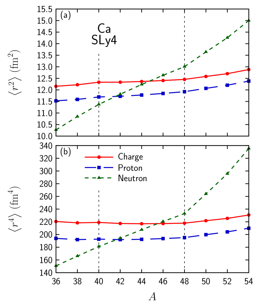
Figure 1: The second $\left\langle{r^{2}}\right\rangle$ and fourth $\left\langle{r^{4}}\right\rangle$ moments of the proton, neutron, and charge density distributions of $\mathrm{Ca}$ isotopes as functions of mass number $A$. They are shown with blue long-dashed, green dashed, and red solid lines, respectively. As an example, the SLy4 functional Chabanat et al. (1998) is used.

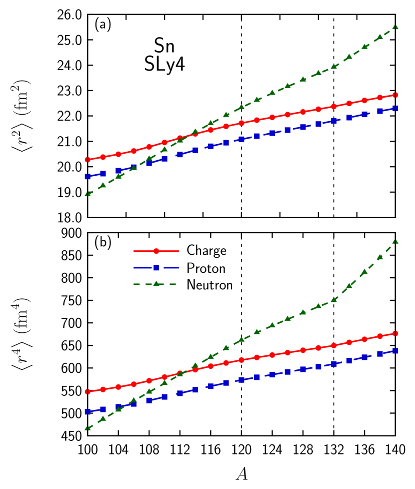
Figure 2: Same as Fig. 1 but for $\mathrm{Sn}$ isotopes.

IV Benchmark calculation

As a benchmark calculation, we test whether the neutron radius calculated theoretically can be reproduced in this novel method. During the benchmark calculation, the theoretical values of $\left\langle{r^{2}}\right\rangle_{\scriptstyle{\text{{{{ch}}}}}}$ and $\left\langle{r^{4}}\right\rangle_{\scriptstyle{\text{{{{ch}}}}}}$ are used, and we will see how accurately $\left\langle{r^{2}}\right\rangle_{n}^{\left(N-2\right)}$ can be calculated from Eq. (9), or how large the neutron slope term and the spin-orbit term or the pairing introduce an uncertainty.

The Skyrme Hartree-Fock-Bogoliubov calculation Vautherin and Brink (1972); Dobaczewski et al. (1984) is performed under the assumption of the axial symmetry using the code hfbtho Navarro Perez et al. (2017). The calculations are performed using a basis of the spherical harmonic oscillator in which $24$ major shells are taken into account and whose oscillator frequency $\omega_{0}$ satisfies $\hbar\omega_{0}=1.2\times 41A^{-1/3}\,\mathrm{MeV}$. As for the proton-proton and neutron-neutron pairing force, a volume-type pairing force Dobaczewski et al. (1984)

$$V_{\scriptstyle{\text{{{{pair}}}}}\tau}\left({\bm{r}},{\bm{r}}^{\prime}\right)=-V_{0\tau}\delta\left({\bm{r}}-{\bm{r}}^{\prime}\right)$$ (10)

is used where the pairing strength $V_{0p}=V_{0n}$ is determined to reproduce the pairing gap of ${}^{120}\mathrm{Sn}$ as $1.4\,\mathrm{MeV}$ with the cutoff energy in quasiparticle space $60\,\mathrm{MeV}$. The SLy4 Chabanat et al. (1998), SLy5 Chabanat et al. (1998), SkM* Bartel et al. (1982), SAMi Roca-Maza et al. (2012), HFB9 Goriely et al. (2005), UNEDF0 Kortelainen et al. (2010), UNEDF1 Kortelainen et al. (2012), and UNEDF2 Kortelainen et al. (2014) EDFs are used as examples, whose pairing strengths $V_{0\tau}$ are $194.2$, $188.2$, $156.2$, $213.7$, $166.4$, $127.6$, $138.4$, and $150.0\,\mathrm{MeV}\,\mathrm{fm}^{3}$, respectively.

Table 1: Benchmark calculation results of $\left\langle{r^{2}}\right\rangle_{\tau}$, $\left\langle{r^{4}}\right\rangle_{\tau}$, $\left\langle{r^{2}}\right\rangle_{\scriptstyle{\text{{{{SO}}}}}\tau}$, $\left\langle{r^{4}}\right\rangle_{\scriptstyle{\text{{{{SO}}}}}\tau}$, $\left\langle{r^{2}}\right\rangle_{\scriptstyle{\text{{{{ch}}}}}}$, and $\left\langle{r^{4}}\right\rangle_{\scriptstyle{\text{{{{ch}}}}}}$. The SLy4 energy density functional Chabanat et al. (1998) is used to calculate $\left\langle{r^{2}}\right\rangle_{\tau}$ and $\left\langle{r^{4}}\right\rangle_{\tau}$. The spin-orbit contributions, $\left\langle{r^{2}}\right\rangle_{\scriptstyle{\text{{{{SO}}}}}\tau}$ and $\left\langle{r^{4}}\right\rangle_{\scriptstyle{\text{{{{SO}}}}}\tau}$, are calculated by using Eqs. (6a) and (7). See the text for detail.

Isotope	Second moments ($\mathrm{fm}^{2}$)					Fourth moments ($\mathrm{fm}^{4}$)
	$\left\langle{r^{2}}\right\rangle_{p}$	$\left\langle{r^{2}}\right\rangle_{n}$	$\left\langle{r^{2}}\right\rangle_{\scriptstyle{\text{{{{SO}}}}}p}$	$\frac{N}{Z}\left\langle{r^{2}}\right\rangle_{\scriptstyle{\text{{{{SO}}}}}n}$	$\left\langle{r^{2}}\right\rangle_{\scriptstyle{\text{{{{ch}}}}}}$	$\left\langle{r^{4}}\right\rangle_{p}$	$\left\langle{r^{4}}\right\rangle_{n}$	$\left\langle{r^{4}}\right\rangle_{\scriptstyle{\text{{{{SO}}}}}p}$	$\frac{N}{Z}\left\langle{r^{4}}\right\rangle_{\scriptstyle{\text{{{{SO}}}}}n}$	$\left\langle{r^{4}}\right\rangle_{\scriptstyle{\text{{{{ch}}}}}}$
${}^{44}\mathrm{Ca}$	$11.778$	$12.234$	$0.000$	$-0.051$	$12.344$	$192.445$	$207.486$	$0.000$	$-1.162$	$216.510$
${}^{46}\mathrm{Ca}$	$11.847$	$12.632$	$0.000$	$-0.075$	$12.377$	$193.613$	$220.471$	$0.000$	$-1.792$	$216.540$
${}^{110}\mathrm{Sn}$	$20.312$	$20.665$	$0.063$	$-0.058$	$20.934$	$535.965$	$565.926$	$2.677$	$-2.320$	$579.136$
${}^{112}\mathrm{Sn}$	$20.483$	$21.020$	$0.063$	$-0.049$	$21.110$	$544.080$	$585.111$	$2.697$	$-1.987$	$587.549$

In this benchmark calculation, first, $\left\langle{r^{2}}\right\rangle_{\tau}$ and $\left\langle{r^{4}}\right\rangle_{\tau}$ are calculated by the hfbtho code, and $\left\langle{r^{2}}\right\rangle_{\scriptstyle{\text{{{{ch}}}}}}$ and $\left\langle{r^{4}}\right\rangle_{\scriptstyle{\text{{{{ch}}}}}}$ are evaluated by using Eqs. (5a), (5b), (6a), and (7). Then, $\left\langle{r^{2}}\right\rangle_{\scriptstyle{\text{{{{ch}}}}}}$ and $\left\langle{r^{4}}\right\rangle_{\scriptstyle{\text{{{{ch}}}}}}$ are assumed to be known, and we test how accurately $\left\langle{r^{2}}\right\rangle_{\tau}$ and $\left\langle{r^{4}}\right\rangle_{\tau}$ can be evaluated. Sources of uncertainty discussed in this paper are estimation of $\left\langle{r^{4}}\right\rangle_{p}$ and the neutron slope term, and if no uncertainty is introduced, evaluated $\left\langle{r^{2}}\right\rangle_{n}$ should be consistent to that calculated by the hfbtho code. The contributions of $\left\langle{r^{2}}\right\rangle_{\scriptstyle{\text{{{{SO}}}}}\tau}$ and $\left\langle{r^{4}}\right\rangle_{\scriptstyle{\text{{{{SO}}}}}\tau}$ are estimated as previously explained and will not play a prominent role in the determination of $\left\langle{r^{2}}\right\rangle_{n}$ when compared with other sources of uncertainties, and thus they are assumed to be known. As examples, the $\mathrm{Ca}$ isotope with $N=26$ and the $\mathrm{Sn}$ isotope with $N=62$ are chosen, i.e., (${}^{44}\mathrm{Ca}$, ${}^{46}\mathrm{Ca}$) and (${}^{110}\mathrm{Sn}$, ${}^{112}\mathrm{Sn}$) pairs are used for Eq. (9). The values calculated with the SLy4 EDF are used. Calculation results of $\left\langle{r^{2}}\right\rangle_{\tau}$ and $\left\langle{r^{4}}\right\rangle_{\tau}$ are shown in Table 1. Using these results, accordingly, we calculate $\left\langle{r^{2}}\right\rangle_{\scriptstyle{\text{{{{SO}}}}}\tau}$, $\left\langle{r^{4}}\right\rangle_{\scriptstyle{\text{{{{SO}}}}}\tau}$, $\left\langle{r^{2}}\right\rangle_{\scriptstyle{\text{{{{ch}}}}}}$, and $\left\langle{r^{4}}\right\rangle_{\scriptstyle{\text{{{{ch}}}}}}$ as shown in Table 1, where $\sum_{a}{\mathcal{N}}_{a\tau}\left\langle{{\bm{l}}\cdot{\bm{\sigma}}}\right\rangle$ are derived from the results of Hartree-Fock-Bogoliubov calculation as shown in Table 2. For comparison, Table 2 shows $\sum_{a}{\mathcal{N}}_{a\tau}\left\langle{{\bm{l}}\cdot{\bm{\sigma}}}\right\rangle$ calculated by using the Hartree-Fock calculation, i.e., integer ${\mathcal{N}}_{a\tau}$. On the one hand, since $\mathrm{Ca}$ and $\mathrm{Sn}$ are proton magic nuclei, the proton pairing does not change $\sum_{a}{\mathcal{N}}_{a\tau}\left\langle{{\bm{l}}\cdot{\bm{\sigma}}}\right\rangle$ for protons. On the other hand, one can find that the neutron pairing affects $\sum_{a}{\mathcal{N}}_{a\tau}\left\langle{{\bm{l}}\cdot{\bm{\sigma}}}\right\rangle$ for neutrons, at most, approximately $30\,\%$, and that the resulting impact on $\left\langle{r^{2}}\right\rangle_{\scriptstyle{\text{{{{ch}}}}}}$ and $\left\langle{r^{4}}\right\rangle_{\scriptstyle{\text{{{{ch}}}}}}$ is eventually less than $0.5\,\%$. Thus, as discussed later, uncertainties associated with the spin-orbit contribution due to the pairing are negligible, and hereinafter, this will not be considered.

Table 2: Spin-orbit expectation values $\sum_{a}{\mathcal{N}}_{a\tau}\left\langle{{\bm{l}}\cdot{\bm{\sigma}}}\right\rangle$ calculated by using the Hartree-Fock-Bogoliubov method. For comparison, those calculated by using the Hartree-Fock method (integer ${\mathcal{N}}_{a\tau}$) are also shown.

Nuclei	Proton $\sum_{a}{\mathcal{N}}_{a\tau}\left\langle{{\bm{l}}\cdot{\bm{\sigma}}}\right\rangle$		Neutron $\sum_{a}{\mathcal{N}}_{a\tau}\left\langle{{\bm{l}}\cdot{\bm{\sigma}}}\right\rangle$
	HF	HFB	HF	HFB
${}^{44}\mathrm{Ca}$	$0$	$0.00$	$+12$	$+11.982$
${}^{46}\mathrm{Ca}$	$0$	$0.00$	$+18$	$+17.860$
${}^{110}\mathrm{Sn}$	$+40$	$+40.00$	$+32$	$+34.492$
${}^{112}\mathrm{Sn}$	$+40$	$+40.00$	$+22$	$+29.025$

Figures 1 and 2, respectively, show $\left\langle{r^{2}}\right\rangle$ and $\left\langle{r^{4}}\right\rangle$ of $\mathrm{Ca}$ and $\mathrm{Sn}$ isotopes calculated with the SLy4 EDF as functions of the mass number $A$. It should be noted that all the calculation results are eventually spherical, although the axial deformation is allowed in the numerical calculations.

IV.1 Derivation of proton fourth moment

Before going into the discussion on the neutron slope term, to derive $\left\langle{r^{2}}\right\rangle_{n}$ from Eqs. (5a) and (5b), $\left\langle{r^{4}}\right\rangle_{p}$ should be estimated in a certain way since it cannot be determined from experimental data, in contrast to $\left\langle{r^{2}}\right\rangle_{p}$. In this paper, we adopt a way which was similar to that used in Ref. Kurasawa et al. (2021).

We estimate the correlation between $\left\langle{r^{2}}\right\rangle_{p}$ and $\left\langle{r^{4}}\right\rangle_{p}$ for ${}^{44}\mathrm{Ca}$, ${}^{46}\mathrm{Ca}$, ${}^{110}\mathrm{Sn}$, and ${}^{112}\mathrm{Sn}$ by using the theoretical results for the selected EDFs as

$$\left\langle{r^{4}}\right\rangle_{p}^{\scriptstyle{\text{{{{Ca-44}}}}}}= \,\left(41.838\pm 1.704\right)\left\langle{r^{2}}\right\rangle_{p}^{\scriptstyle{\text{{{{Ca-44}}}}}}$$

$$\,-\left(300.062\pm 19.920\right)\qquad\text{($r=0.9951$)},$$ (11a)

$$\left\langle{r^{4}}\right\rangle_{p}^{\scriptstyle{\text{{{{Ca-46}}}}}}= \,\left(45.559\pm 2.760\right)\left\langle{r^{2}}\right\rangle_{p}^{\scriptstyle{\text{{{{Ca-46}}}}}}$$

$$\,-\left(345.755\pm 32.458\right)\qquad\text{($r=0.9892$)},$$ (11b)

$$\left\langle{r^{4}}\right\rangle_{p}^{\scriptstyle{\text{{{{Sn-110}}}}}}= \,\left(56.585\pm 6.607\right)\left\langle{r^{2}}\right\rangle_{p}^{\scriptstyle{\text{{{{Sn-110}}}}}}$$

$$\,-\left(614.296\pm 133.676\right)\qquad\text{($r=0.9614$)},$$ (11c)

$$\left\langle{r^{4}}\right\rangle_{p}^{\scriptstyle{\text{{{{Sn-112}}}}}}= \,\left(59.223\pm 7.461\right)\left\langle{r^{2}}\right\rangle_{p}^{\scriptstyle{\text{{{{Sn-112}}}}}}$$

$$\,-\left(669.781\pm 152.183\right)\qquad\text{($r=0.9555$)},$$ (11d)

respectively, as shown in Fig. 3. The proton second moments extracted from experimental charge radii Angeli and Marinova (2013), experimental nucleon second moments ($r_{\scriptstyle{\text{{{{E}}}}}p}=0.8409\pm 0.0004\,\mathrm{fm}$ and $r_{\scriptstyle{\text{{{{E}}}}}n}^{2}=-0.1161\pm 0.0022\,\mathrm{fm}^{2}$) Zyla et al. (2020), and Eq. (5a) are also shown as filled bands where Hartree-Fock (integer) occupations are used for ${\mathcal{N}}_{a\tau}$. Given that the estimated values of $\left\langle{r^{2}}\right\rangle_{p}$ shown in Table 1 are $\left\langle{r^{2}}\right\rangle_{p}^{\scriptstyle{\text{{{{Ca-44}}}}}}=11.778\,\mathrm{fm}^{2}$, $\left\langle{r^{2}}\right\rangle_{p}^{\scriptstyle{\text{{{{Ca-46}}}}}}=11.847\,\mathrm{fm}^{2}$, $\left\langle{r^{2}}\right\rangle_{p}^{\scriptstyle{\text{{{{Sn-110}}}}}}=20.312\,\mathrm{fm}^{2}$, and $\left\langle{r^{2}}\right\rangle_{p}^{\scriptstyle{\text{{{{Sn-112}}}}}}=20.483\,\mathrm{fm}^{2}$, we infer that the estimated values of $\left\langle{r^{4}}\right\rangle_{p}$ for ${}^{44}\mathrm{Ca}$, ${}^{46}\mathrm{Ca}$, ${}^{110}\mathrm{Sn}$, and ${}^{112}\mathrm{Sn}$ are $192.716\pm 1.993\,\mathrm{fm}^{4}$, $193.980\pm 4.800\,\mathrm{fm}^{4}$, $535.091\pm 37.198\,\mathrm{fm}^{4}$, and $543.317\pm 45.483\,\mathrm{fm}^{4}$, respectively. These uncertainties are theoretical ones coming from the linear fits. These uncertainties range from $1.03\,\%$ to $8.37\,\%$ and these deviations from the benchmark values are around $0.15\,\%$. These good correlations ($r\gtrsim 0.95$) are due to the fact that the density profiles calculated with different EDFs share similar properties due to shell and orbital structures.

Despite the good correlations between $\left\langle{r^{2}}\right\rangle_{p}$ and $\left\langle{r^{4}}\right\rangle_{p}$, the final values of $\left\langle{r^{2}}\right\rangle_{n}$ calculated by using Eq. (5b), or rearranged equation,

$$\left\langle{r^{2}}\right\rangle_{n}= \,\frac{3Z}{10Nr_{\scriptstyle{\text{{{{E}}}}}n}^{2}}\left[\left\langle{r^{4}}\right\rangle_{\scriptstyle{\text{{{{ch}}}}}}-\left\langle{r^{4}}\right\rangle_{p}-\frac{10}{3}r_{\scriptstyle{\text{{{{E}}}}}p}^{2}\left\{\left\langle{r^{2}}\right\rangle_{\scriptstyle{\text{{{{ch}}}}}}-\left(r_{\scriptstyle{\text{{{{E}}}}}p}^{2}+\frac{N}{Z}r_{\scriptstyle{\text{{{{E}}}}}n}^{2}\right)-\left\langle{r^{2}}\right\rangle_{\scriptstyle{\text{{{{SO}}}}}p}-\frac{N}{Z}\left\langle{r^{2}}\right\rangle_{\scriptstyle{\text{{{{SO}}}}}n}\right\}\right.$$

$$\,\left.-\left(r_{\scriptstyle{\text{{{{E}}}}}p}^{4}+\frac{N}{Z}r_{\scriptstyle{\text{{{{E}}}}}n}^{4}\right)-\left\langle{r^{4}}\right\rangle_{\scriptstyle{\text{{{{SO}}}}}p}-\frac{N}{Z}\left\langle{r^{4}}\right\rangle_{\scriptstyle{\text{{{{SO}}}}}n}\right],$$ (12)

are $\left\langle{r^{2}}\right\rangle_{n}^{\scriptstyle{\text{{{{Ca-44}}}}}}=12.842\pm 4.470\,\mathrm{fm}^{2}$ and $\left\langle{r^{2}}\right\rangle_{n}^{\scriptstyle{\text{{{{Sn-110}}}}}}=18.706\pm 83.434\,\mathrm{fm}^{2}$, and, consequently, $\sqrt{\left\langle{r^{2}}\right\rangle_{n}^{\scriptstyle{\text{{{{Ca-44}}}}}}}=3.584\pm 0.624\,\mathrm{fm}$ and $\sqrt{\left\langle{r^{2}}\right\rangle_{n}^{\scriptstyle{\text{{{{Sn-110}}}}}}}=4.325\pm 9.645\,\mathrm{fm}$, respectively, whereas the benchmarked values are $\sqrt{\left\langle{r^{2}}\right\rangle_{n}^{\scriptstyle{\text{{{{Ca-44}}}}}}}=3.498\,\mathrm{fm}$ and $\sqrt{\left\langle{r^{2}}\right\rangle_{n}^{\scriptstyle{\text{{{{Sn-110}}}}}}}=4.546\,\mathrm{fm}$. The uncertainties range from $17\,\%$ to $220\,\%$. This means the uncertainty is too large to extract $\Delta r_{np}$ or even $\sqrt{\left\langle{r^{2}}\right\rangle_{n}}$. The reason why the error of $\left\langle{r^{2}}\right\rangle_{n}$ enhances is due to the coefficient of $\left\langle{r^{4}}\right\rangle_{p}$, that is, $3Z/\left|10Nr_{\scriptstyle{\text{{{{E}}}}}n}^{2}\right|\gtrsim 2.69\,\mathrm{fm}^{-2}$.

In short, extracting $\left\langle{r^{2}}\right\rangle_{n}$ from the charge second and fourth moments is not feasible, unless the proton fourth moment $\left\langle{r^{4}}\right\rangle_{p}$ can also be determined precisely either experimentally or theoretically.

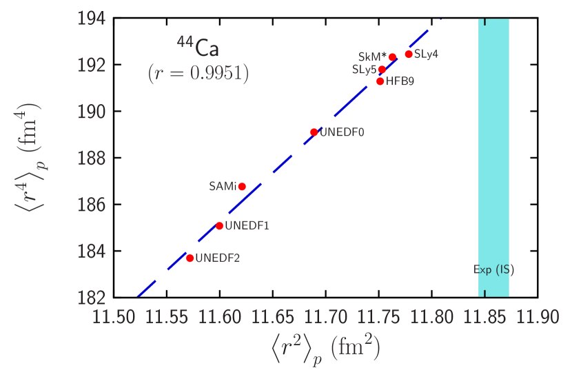
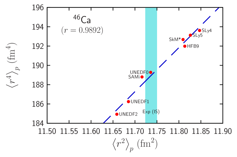
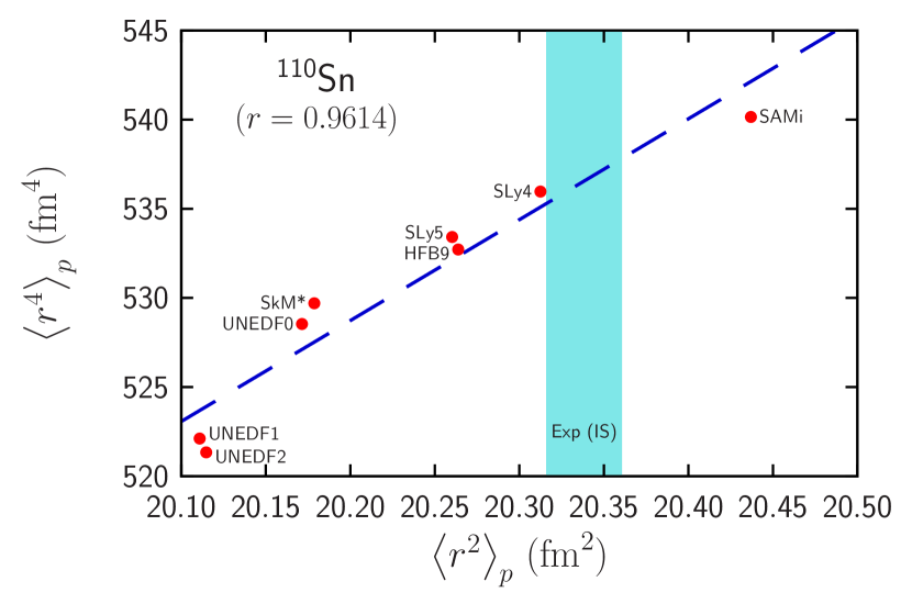
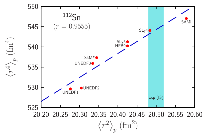
Figure 3: Correlation of proton second and fourth moments, $\left\langle{r^{2}}\right\rangle_{p}$ and $\left\langle{r^{4}}\right\rangle_{p}$ for ${}^{44}\mathrm{Ca}$, ${}^{46}\mathrm{Ca}$, ${}^{110}\mathrm{Sn}$, and ${}^{112}\mathrm{Sn}$. The proton second moments extracted from experimental charge radii measured by using isotope shift (IS) method Angeli and Marinova (2013) and Eq. (5a) are also shown as filled bands. See the text for more details.

IV.2 Neutron slope term and isotope-shift method

In the previous section, we see that extracting $\left\langle{r^{2}}\right\rangle_{n}$ from $\left\langle{r^{2}}\right\rangle_{\scriptstyle{\text{{{{ch}}}}}}$ and $\left\langle{r^{4}}\right\rangle_{\scriptstyle{\text{{{{ch}}}}}}$ may not be feasible. Nevertheless, in this section, the other method called the isotope-shift method, which is introduced in Sec. III, will be further discussed since once $\left\langle{r^{4}}\right\rangle_{p}$ is determined precisely, the method helps us to reduce uncertainty. Furthermore, in laser spectroscopic experiments, the difference in $\left\langle{r^{2}}\right\rangle_{\scriptstyle{\text{{{{ch}}}}}}$ between two isotopes is obtained whereas absolute values are not. Thus, this isotope-shift method is still important for discussion.

The neutron slope term for $\mathrm{Ca}$ and $\mathrm{Sn}$ isotopes are derived by the average of $32$ and $80$ results, which are for $N=22$, $24$, $26$, and $28$ ($\mathrm{Ca}$ isotopes) or $N=52$, $54$, $56$, …, $70$ ($\mathrm{Sn}$ isotopes) calculated with the selected eight functionals, i.e., SLy4, SLy5, SkM*, SAMi, HFB9, UNEDF0, UNEDF1, and UNEDF2 . The calculated value of $N\left(\left\langle{r^{2}}\right\rangle_{n}^{\left(N\right)}-\left\langle{r^{2}}\right\rangle_{n}^{\left(N-2\right)}\right)$ is

$$N\left(\left\langle{r^{2}}\right\rangle_{n}^{\left(N\right)}-\left\langle{r^{2}}\right\rangle_{n}^{\left(N-2\right)}\right)$$

$$=\begin{cases}10.720\pm 1.155\,\mathrm{fm}^{2}&\text{for $\mathrm{Ca}$ isotopes},\\ 20.614\pm 2.086\,\mathrm{fm}^{2}&\text{for $\mathrm{Sn}$ isotopes},\end{cases}$$ (13)

respectively. Substituting the neutron slope term [Eq. (13)] and $\left\langle{r^{4}}\right\rangle_{p}$ calculated in Sec. IV.1 as well as $\left\langle{r^{4}}\right\rangle_{\scriptstyle{\text{{{{ch}}}}}}$ and $\left\langle{r^{2}}\right\rangle_{p}$ shown in Table 1, into Eq. (9), we get $\left\langle{r^{2}}\right\rangle_{n}$ of ${}^{44}\mathrm{Ca}$ and ${}^{110}\mathrm{Sn}$ as

$$\left\langle{r^{2}}\right\rangle_{n}^{\scriptstyle{\text{{{{Ca-44}}}}}} =14.639\pm 139.880\,\mathrm{fm}^{2},$$ (14a)

$$\left\langle{r^{2}}\right\rangle_{n}^{\scriptstyle{\text{{{{Sn-110}}}}}} =28.774\pm 3953.686\,\mathrm{fm}^{2},$$ (14b)

respectively, where breakdown of these uncertainties are shown in Table 3. Accordingly, the neutron radii are calculated as

$$\sqrt{\left\langle{r^{2}}\right\rangle_{n}^{\scriptstyle{\text{{{{Ca-44}}}}}}} =3.826\pm 18.280\,\mathrm{fm},$$ (15a)

$$\sqrt{\left\langle{r^{2}}\right\rangle_{n}^{\scriptstyle{\text{{{{Sn-110}}}}}}} =5.364\pm 368.531\,\mathrm{fm}.$$ (15b)

Obviously, the uncertainties are too large to extract $\left\langle{r^{2}}\right\rangle_{n}$ and $\sqrt{\left\langle{r^{2}}\right\rangle_{n}}$. Note that the errors that are shown here are simply standard deviations. For more details, see Appendix C.

Contribution to these standard deviations can be divided into two parts: the part that originates from $\left\langle{r^{4}}\right\rangle_{p}$ and that from the neutron slope term. Other sources can be considered as negligible. Contribution of the neutron slope term to the total standard deviation $\sigma^{2}$ is approximately $2\,\mathrm{ppm}$ or less. If there were no uncertainties due to $\left\langle{r^{4}}\right\rangle_{p}$, the results would become much improved as

$$\left\langle{r^{2}}\right\rangle_{n}^{\scriptstyle{\text{{{{Ca-44}}}}}} =12.054\pm 0.578\,\mathrm{fm}^{2},$$ (16a)

$$\left\langle{r^{2}}\right\rangle_{n}^{\scriptstyle{\text{{{{Sn-110}}}}}} =21.348\pm 1.043\,\mathrm{fm}^{2}.$$ (16b)

Thus, the assumption for the neutron slope term is reasonable, whereas the estimation of $\left\langle{r^{4}}\right\rangle_{p}$ remains a problem.

As an important remark, it should be noted that $r_{\scriptstyle{\text{{{{E}}}}}n}^{2}$ and $r_{\scriptstyle{\text{{{{E}}}}}n}^{4}$ include the information of the charge distribution of the neutron, which has been determined with large uncertainty. However, in the isotope-shift method proposed in this paper, most of the contributions from these terms are canceled out in Eq. (9). In the last subsection of this section, discussion for uncertainty due to the nucleon form factors will be given.

Table 3: Breakdown of uncertainties of isotope-shift method [Eq. (9)]. Uncertainties are calculated by using standard deviations. For comparison, those of direct method is also shown. Uncertainties due to nucleon second and fourth moments $r_{\scriptstyle{\text{{{{E}}}}}\tau}^{2}$ and $r_{\scriptstyle{\text{{{{E}}}}}\tau}^{4}$ (column with *) are not considered in the total uncertainties. See the text for more details.

Nuclei	Method	$\sigma^{2}$ ($\mathrm{fm}^{4}$)				$\sigma$ ($\mathrm{fm}^{2}$)	$\left\langle{r^{2}}\right\rangle_{n}$ ($\mathrm{fm}^{2}$)
		$r_{\scriptstyle{\text{{{{E}}}}}\tau}^{n}$ (*)	$\left\langle{r^{4}}\right\rangle_{p}$	Neutron slope term	Total		Calculation	Benchmark
${}^{44}\mathrm{Ca}$	Direct	$9.934$	$19.977$	—	$19.977$	$4.470$	$12.842$	$12.234$
	Isotope-shift	$0.667$	$19566.142$	$0.334$	$19566.476$	$139.880$	$14.639$	$12.234$
${}^{110}\mathrm{Sn}$	Direct	$31.137$	$6961.160$	—	$6961.160$	$83.434$	$18.706$	$20.665$
	Isotope-shift	$4.091$	$15631629.395$	$1.087$	$15631630.482$	$3953.686$	$28.774$	$20.665$

IV.3 Uncertainty due to nucleon form factors

Here, uncertainty due to nucleon form factors, which is not considered in evaluations of $\left\langle{r^{2}}\right\rangle_{n}$ in the previous subsections, is discussed. Note that, in this subsection, we do not consider the uncertainty discussed in the previous subsections.

In general, $\left\langle{r^{2}}\right\rangle_{n}$ can be regarded as a function of $r_{\scriptstyle{\text{{{{E}}}}}\tau}^{2}$ and $r_{\scriptstyle{\text{{{{E}}}}}\tau}^{4}$. Accordingly, the uncertainty due to the nucleon form factors can be calculated as

$$\sigma^{2}_{\scriptstyle{\text{{{{form}}}}}}\lesssim\left(\frac{\partial\left\langle{r^{2}}\right\rangle_{n}}{\partial r_{\scriptstyle{\text{{{{E}}}}}p}^{2}}\right)^{2}\sigma_{r_{\scriptscriptstyle{\text{{{{E}}}}}p}^{2}}^{2}+\left(\frac{\partial\left\langle{r^{2}}\right\rangle_{n}}{\partial r_{\scriptstyle{\text{{{{E}}}}}p}^{4}}\right)^{2}\sigma_{r_{\scriptscriptstyle{\text{{{{E}}}}}p}^{4}}^{2}+\left(\frac{\partial\left\langle{r^{2}}\right\rangle_{n}}{\partial r_{\scriptstyle{\text{{{{E}}}}}n}^{2}}\right)^{2}\sigma_{r_{\scriptscriptstyle{\text{{{{E}}}}}n}^{2}}^{2}+\left(\frac{\partial\left\langle{r^{2}}\right\rangle_{n}}{\partial r_{\scriptstyle{\text{{{{E}}}}}n}^{4}}\right)^{2}\sigma_{r_{\scriptscriptstyle{\text{{{{E}}}}}n}^{4}}^{2},$$ (17)

where contributions of the magnetic form factors are neglected since they are tiny. Here, contributions from the covariances are also neglected, and, because of this, the uncertainty is overestimated slightly.

The uncertainty due to the nucleon form factors for the direct method [Eq. (12)] can be estimated as

$$\sigma_{\left\langle{r^{2}}\right\rangle_{n}}^{2}\lesssim\left[\frac{Z}{N}\frac{1}{r_{\scriptstyle{\text{{{{E}}}}}n}^{2}}\left(\left\langle{r^{2}}\right\rangle_{p}-r_{\scriptstyle{\text{{{{E}}}}}p}^{2}\right)\right]^{2}\sigma_{r_{\scriptscriptstyle{\text{{{{E}}}}}p}^{2}}^{2}+\left(\frac{Z}{N}\frac{3}{10r_{\scriptstyle{\text{{{{E}}}}}n}^{2}}\right)^{2}\sigma_{r_{\scriptscriptstyle{\text{{{{E}}}}}p}^{4}}^{2}+\left[\frac{1}{r_{\scriptstyle{\text{{{{E}}}}}n}^{2}}\left(\left\langle{r^{2}}\right\rangle_{n}-r_{\scriptstyle{\text{{{{E}}}}}p}^{2}\right)\right]^{2}\sigma_{r_{\scriptscriptstyle{\text{{{{E}}}}}n}^{2}}^{2}+\left(\frac{3}{10r_{\scriptstyle{\text{{{{E}}}}}n}^{2}}\right)^{2}\sigma_{r_{\scriptscriptstyle{\text{{{{E}}}}}n}^{4}}^{2},$$ (18)

whereas the uncertainty due to the nucleon form factors for the isotope-shift method [Eq. (9)] can be estimated as

$$\sigma_{\left\langle{r^{2}}\right\rangle_{n}}^{2}\lesssim \,\left[1-\frac{Z}{r_{\scriptstyle{\text{{{{E}}}}}n}^{2}}\frac{\left\langle{r^{2}}\right\rangle_{\scriptstyle{\text{{{{ch}}}}}}^{\left(N\right)}-\left\langle{r^{2}}\right\rangle_{\scriptstyle{\text{{{{ch}}}}}}^{\left(N-2\right)}}{2}-\frac{\kappa_{n}}{M_{n}^{2}}\frac{1}{r_{\scriptstyle{\text{{{{E}}}}}n}^{2}}\left\langle{{\bm{l}}\cdot{\bm{\sigma}}}\right\rangle_{n\scriptstyle{\text{{{{last}}}}}}\right]^{2}\sigma_{r_{\scriptscriptstyle{\text{{{{E}}}}}p}^{2}}^{2}$$

$$\,+\left[\frac{1}{r_{\scriptstyle{\text{{{{E}}}}}n}^{2}}\left(\left\langle{r^{2}}\right\rangle_{n}^{\left(N-2\right)}+N\frac{\left\langle{r^{2}}\right\rangle_{n}^{\left(N\right)}-\left\langle{r^{2}}\right\rangle_{n}^{\left(N-2\right)}}{2}-r_{\scriptstyle{\text{{{{E}}}}}p}^{2}\right)\right]^{2}\sigma_{r_{\scriptscriptstyle{\text{{{{E}}}}}n}^{2}}^{2}+\left(\frac{3}{10}\frac{1}{r_{\scriptstyle{\text{{{{E}}}}}n}^{2}}\right)^{2}\sigma_{r_{\scriptscriptstyle{\text{{{{E}}}}}n}^{4}}^{2}.$$ (19)

For simplicity, here relative uncertainty $\sigma_{r_{\scriptscriptstyle{\text{{{{E}}}}}\tau}^{n}}/r_{\scriptstyle{\text{{{{E}}}}}\tau}^{n}$, is assumed $5\,\%$. The uncertainties calculated by Eq. (18) for ${}^{44}\mathrm{Ca}$ and ${}^{110}\mathrm{Sn}$ are $\sigma^{2}_{\left\langle{r^{2}}\right\rangle_{n}}=9.934\,\mathrm{fm}^{4}$ and $31.137\,\mathrm{fm}^{4}$, respectively. If one uses the isotope-shift method, the uncertainties are further suppressed as $\sigma^{2}_{\left\langle{r^{2}}\right\rangle_{n}}=0.667\,\mathrm{fm}^{4}$ and $4.091\,\mathrm{fm}^{4}$, respectively. Thus, the isotope-shift method has another advantage to suppress the uncertainty due to the nucleon form factors. These errors are anyway negligible as compared to the error introduced by the correlation (that is, their covariance) between $\left\langle{r^{2}}\right\rangle_{p}$ and $\left\langle{r^{4}}\right\rangle_{p}$.

V Conclusion

In this paper, we have discussed how to extract the neutron radius, that is, the second moment of the neutron distribution by using the experimentally measured second and fourth moments of the charge distribution. Our goal was to reduce model assumptions to a minimum. To this aim, we have discussed in detail two contributions to the neutron moment: the spin-orbit contribution and the contribution from the fourth moment of the proton distribution. As for this latter, we have seen we can relate it to the second moment in a quite robust manner. Therefore, we deem that we have been able to determine the mildest assumptions under which the neutron radius of a single isotope can be extracted.

Our main result has been the introduction of a novel method to extract neutron radius from the charge density distribution using the information of two neighboring even-even nuclei. In this method, the uncertainties due to nucleon form factors and introduced by approximation for spin-orbit contribution are suppressed, whereas the uncertainties introduced by the pairing are negligible. We advocate that this method, namely the consideration of two neighboring isotopes, is more reliable.

Despite our efforts, we conclude that the main obstacle to an accurate determination of the neutron radius is the contribution from the proton fourth moment. Even if this is strongly correlated to the second moment, the resulting uncertainty cannot be neglected. This uncertainty is strongly enhanced when propagated from the fourth moment to the neutron radius. Eventually, extracting the neutron radius or the neutron-skin thickness from the second and fourth moments of the charge density distribution does not seem to be feasible based on the present discussion. Despite these pessimistic conclusions, the equations derived in this paper may be useful for further understanding and investigation and even more useful if, in the future, a clever way to better determine the proton fourth moment can be envisaged.

Appendix A Derivation of Eq. (4)

In this appendix, we recall the way to derive Eq. (4), which was originally derived by Kurasawa and Suzuki Kurasawa and Suzuki (2019). Here, the unnormalized $2n$th moment of a density $\rho$ can be calculated as

$$\int\rho\left({\bm{r}}\right)\,r^{2n}\,d{\bm{r}} =\int\left\{\frac{1}{\left(2\pi\right)^{3}}\int\left[\left(-\operatorname{\Delta}_{{\bm{q}}}\right)^{n}\tilde{\rho}\left({\bm{q}}\right)\right]e^{i{\bm{q}}\cdot{\bm{r}}}\,d{\bm{q}}\right\}d{\bm{r}}$$

$$=\int\left[\left(-\operatorname{\Delta}_{{\bm{q}}}\right)^{n}\tilde{\rho}\left({\bm{q}}\right)\right]\left[\int\frac{1}{\left(2\pi\right)^{3}}e^{-i\left(-{\bm{q}}\right)\cdot{\bm{r}}}\,d{\bm{r}}\right]d{\bm{q}}$$

$$=\int\left[\left(-\operatorname{\Delta}_{{\bm{q}}}\right)^{n}\tilde{\rho}\left({\bm{q}}\right)\right]\tilde{\delta}\left(-{\bm{q}}\right)\,d{\bm{q}}$$

$$=\left[\left(-\operatorname{\Delta}_{{\bm{q}}}\right)^{n}\tilde{\rho}\left({\bm{q}}\right)\right]_{{\bm{q}}={\bm{0}}},$$ (20)

and hence

$$\left\langle{r^{2n}}\right\rangle =\frac{\left[\left(-\operatorname{\Delta}_{{\bm{q}}}\right)^{n}\tilde{\rho}\left({\bm{q}}\right)\right]_{{\bm{q}}={\bm{0}}}}{\tilde{\rho}\left({\bm{0}}\right)}$$

$$=\frac{1}{N_{\tau}}\left[\left(-\operatorname{\Delta}_{{\bm{q}}}\right)^{n}\tilde{\rho}\left({\bm{q}}\right)\right]_{{\bm{q}}={\bm{0}}},$$ (21)

holds Kurasawa and Suzuki (2019). Since the Laplacian of a function $f$ is written as

$$\operatorname{\Delta}f\left(r\right) =\frac{d^{2}f\left(r\right)}{dr^{2}}+\frac{2}{r}\frac{df\left(r\right)}{dr}$$

$$=\frac{1}{r}\frac{d^{2}}{dr^{2}}\left[rf\left(r\right)\right],$$ (22)

as long as $f$ is spherically symmetric, Eq. (20) can be simplified as

$$\left[\left(-\operatorname{\Delta}_{{\bm{q}}}\right)^{n}\tilde{\rho}_{\scriptstyle{\text{{{{ch}}}}}}\left({\bm{q}}\right)\right]_{{\bm{q}}={\bm{0}}} =\left(-1\right)^{n}\left\{\frac{1}{q}\frac{d^{2n}}{dq^{2n}}\left[q\sum_{\tau}\tilde{G}_{\scriptstyle{\text{{{{E}}}}}\tau}\left(q^{2}\right)\tilde{\rho}_{\tau}\left(q\right)\right]\right\}_{q=0}$$

$$=\left(-1\right)^{n}4\pi\left\{\frac{1}{q}\frac{d^{2n}}{dq^{2n}}\left[q\sum_{\tau}\tilde{G}_{\scriptstyle{\text{{{{E}}}}}\tau}\left(q^{2}\right)\,\int_{0}^{\infty}\rho_{\tau}\left(r\right)\,\frac{\sin\left(qr\right)}{qr}r^{2}\,dr\right]\right\}_{q=0}$$

$$=\left(-1\right)^{n}4\pi\sum_{\tau}\int_{0}^{\infty}\left\{\frac{1}{q}\frac{d^{2n}}{dq^{2n}}\tilde{G}_{\scriptstyle{\text{{{{E}}}}}\tau}\left(q^{2}\right)\,\sin\left(qr\right)\right\}_{q=0}\rho_{\tau}\left(r\right)\,r\,dr.$$ (23)

Thus, combining with Eq. (21) and assuming the spherical symmetry, we get Eq. (4) for $\rho_{\scriptstyle{\text{{{{ch}}}}}}$.

Appendix B Charge form factor of the nucleus

In this appendix, the detailed derivations of equations for the second and fourth moments discussed in Sec. II are shown. The spin-orbit contributions to $\left\langle{r^{2}}\right\rangle_{\scriptstyle{\text{{{{ch}}}}}}$ and $\left\langle{r^{4}}\right\rangle_{\scriptstyle{\text{{{{ch}}}}}}$ are discussed as well. For the contribution to $\left\langle{r^{2}}\right\rangle_{\scriptstyle{\text{{{{ch}}}}}}$, it has been already derived by Horowitz and Piekarewicz Horowitz and Piekarewicz (2012). Nevertheless, the contribution to $\left\langle{r^{4}}\right\rangle_{\scriptstyle{\text{{{{ch}}}}}}$ can be derived in the parallel way as that to $\left\langle{r^{2}}\right\rangle_{\scriptstyle{\text{{{{ch}}}}}}$, and, thus, the derivation of the former is also shown here for convenience.

The Dirac and Pauli form factors of nucleons are denoted by $\tilde{F}_{1\tau}$ and $\tilde{F}_{2\tau}$, and the Sachs electric and magnetic form factors are defined by Cloët et al. (2009)

$$\tilde{G}_{\scriptstyle{\text{{{{E}}}}}\tau}\left(Q^{2}\right) =\tilde{F}_{1\tau}\left(Q^{2}\right)-\frac{Q^{2}}{4M_{\tau}^{2}}\tilde{F}_{2\tau}\left(Q^{2}\right),$$ (24a)

$$\tilde{G}_{\scriptstyle{\text{{{{M}}}}}\tau}\left(Q^{2}\right) =\tilde{F}_{1\tau}\left(Q^{2}\right)+\tilde{F}_{2\tau}\left(Q^{2}\right),$$ (24b)

respectively, in the relativistic scheme, where $Q^{2}=-q_{\mu}q^{\mu}>0$ and $M_{\tau}$ is the nucleon mass. The Dirac and Pauli form factors are normalized as

$$\tilde{F}_{1\tau}\left(0\right) =e_{\tau},$$ (25a)

$$\tilde{F}_{2\tau}\left(0\right) =\mu_{\tau},$$ (25b)

respectively, where $e_{\tau}$ and $\mu_{\tau}$ denote the charge and the magnetic dipole moment of nucleons $\tau$. The anomalous magnetic moment $\kappa_{\tau}$ reads $\kappa_{\tau}=\mu_{\tau}-e_{\tau}$. Accordingly, the electric and magnetic form factors are normalized as

$$\tilde{G}_{\scriptstyle{\text{{{{E}}}}}p}\left(0\right) =1,$$ (26a)

$$\tilde{G}_{\scriptstyle{\text{{{{E}}}}}n}\left(0\right) =0,$$ (26b)

$$\tilde{G}_{\scriptstyle{\text{{{{M}}}}}\tau}\left(0\right) =\mu_{\tau}.$$ (26c)

Throughout the derivation of the charge form factors, the relativistic scheme is used. The relativistic single-particle (Kohn-Sham) orbital under the spherically symmetric potential is written as

$$\varphi_{a\tau}\left({\bm{r}}\right)=\frac{1}{r}\begin{pmatrix}ig_{a\tau}\left(r\right)\\ f_{a\tau}\left(r\right){\bm{\sigma}}\cdot\hat{{\bm{r}}}\end{pmatrix}{\mathcal{Y}}_{a}\left(\theta,\varphi\right)\chi_{\tau},$$ (27)

where $\hat{{\bm{r}}}={\bm{r}}/r$, ${\mathcal{Y}}_{a}$ is the spherical spinor, $\chi_{\tau}$ is the isospin spinor, and the set of the quantum numbers $a=\left(n,\kappa,m\right)$ includes the principal quantum number $n$, the angular quantum number,

$$\kappa=\begin{cases}+\left(j+1/2\right)&\text{(for $j=l-1/2$)},\\ -\left(j+1/2\right)&\text{(for $j=l+1/2$)},\end{cases}$$ (28)

and its $z$-projection $m$ Meng et al. (2006); Nikšić et al. (2011); Liang et al. (2015). The normalization condition

$$\int\varphi_{a\tau}^{\dagger}\left({\bm{r}}\right)\varphi_{a\tau}\left({\bm{r}}\right)\,d{\bm{r}} =\int_{0}^{\infty}\left[\left\{g_{a\tau}\left(r\right)\right\}^{2}+\left\{f_{a\tau}\left(r\right)\right\}^{2}\right]\,dr$$

$$=1$$ (29)

holds.

The matrix element of the electromagnetic current operator for nucleon $\tau$, $\hat{J}^{\mu}_{\scriptstyle{\text{{{{EM}}}}}\tau}$, reads de Forest Jr. and Walecka (1966); Donnelly and Walecka (1975); Friar and Negele (1975); Musolf et al. (1994)

$$\hat{J}^{\mu}_{\scriptstyle{\text{{{{EM}}}}}\tau}\left(Q^{2}\right)=\tilde{G}_{\scriptstyle{\text{{{{E}}}}}\tau}\left(Q^{2}\right)\gamma^{\mu}+\frac{\tilde{G}_{\scriptstyle{\text{{{{M}}}}}\tau}\left(Q^{2}\right)-\tilde{G}_{\scriptstyle{\text{{{{E}}}}}\tau}\left(Q^{2}\right)}{1+Q^{2}/4M_{\tau}^{2}}\left(\frac{Q^{2}}{4M_{\tau}^{2}}\gamma^{\mu}+i\sigma^{\mu\nu}\frac{q_{\nu}}{2M_{\tau}}\right)$$ (30)

and especially its $\mu=0$ component (density component) is

$$\hat{J}^{0}_{\scriptstyle{\text{{{{EM}}}}}\tau}\left(Q^{2}\right)=\tilde{G}_{\scriptstyle{\text{{{{E}}}}}\tau}\left(Q^{2}\right)\gamma^{0}+\frac{\tilde{G}_{\scriptstyle{\text{{{{M}}}}}\tau}\left(Q^{2}\right)-\tilde{G}_{\scriptstyle{\text{{{{E}}}}}\tau}\left(Q^{2}\right)}{1+Q^{2}/4M_{\tau}^{2}}\left(\frac{Q^{2}}{4M_{\tau}^{2}}\gamma^{0}+\gamma^{0}\frac{{\bm{\gamma}}\cdot{\bm{q}}}{2M_{\tau}}\right).$$ (31)

Since one-nucleon contribution of the form factors is defined by $\left\langle{N_{\tau}\left(p^{\prime}\right)}\middle|{\hat{J}_{\scriptstyle{\text{{{{EM}}}}}\tau}^{0}\left(Q^{2}\right)}\middle|{N_{\tau}\left(p\right)}\right\rangle$ with the on-shell nucleon state $\left|{N_{\tau}\left(p\right)}\right\rangle$ and four-momentum transfer $Q=p^{\prime}-p$, the charge form factor of the nucleus $\tilde{\rho}_{\scriptstyle{\text{{{{ch}}}}}}$ is calculated by summing up the single-nucleon contributions as

$$\tilde{\rho}_{\scriptstyle{\text{{{{ch}}}}}}\left(q\right) \simeq\sum_{\text{occ}}\left\langle{N_{\tau}\left(p^{\prime}\right)}\middle|{\hat{J}_{\scriptstyle{\text{{{{EM}}}}}\tau}^{0}\left(Q^{2}\right)}\middle|{N_{\tau}\left(p\right)}\right\rangle$$

$$=\sum_{\tau=p,\,n}\sum_{a}\iint\varphi_{a\tau}^{\dagger}\left({\bm{r}}^{\prime}\right)e^{i{\bm{p}}^{\prime}\cdot{\bm{r}}^{\prime}}\delta\left({\bm{r}}-{\bm{r}}^{\prime}\right){\hat{J}_{\scriptstyle{\text{{{{EM}}}}}\tau}^{0}\left(Q^{2}\right)}\varphi_{a\tau}\left({\bm{r}}\right)e^{-i{\bm{p}}\cdot{\bm{r}}}\,d{\bm{r}}\,d{\bm{r}}^{\prime}$$

$$\simeq\sum_{\tau=p,\,n}\sum_{a}\iint\varphi_{a\tau}^{\dagger}\left({\bm{r}}^{\prime}\right)e^{i{\bm{p}}^{\prime}\cdot{\bm{r}}^{\prime}}\delta\left({\bm{r}}-{\bm{r}}^{\prime}\right){\hat{J}_{\scriptstyle{\text{{{{EM}}}}}\tau}^{0}\left(q^{2}\right)}\varphi_{a\tau}\left({\bm{r}}\right)e^{-i{\bm{p}}\cdot{\bm{r}}}\,d{\bm{r}}\,d{\bm{r}}^{\prime}$$

$$=\sum_{\tau=p,\,n}\sum_{a}\int\varphi_{a\tau}^{\dagger}\left({\bm{r}}\right){\hat{J}_{\scriptstyle{\text{{{{EM}}}}}\tau}^{0}\left(q^{2}\right)}\varphi_{a\tau}\left({\bm{r}}\right)e^{-i{\bm{q}}\cdot{\bm{r}}}\,d{\bm{r}}$$

$$=\sum_{\tau=p,\,n}\left[\tilde{G}_{\scriptstyle{\text{{{{E}}}}}\tau}\left(q^{2}\right)\tilde{F}_{\scriptstyle{\text{{{{V}}}}}\tau}\left(q\right)+\frac{\tilde{G}_{\scriptstyle{\text{{{{M}}}}}}\left(q^{2}\right)-\tilde{G}_{\scriptstyle{\text{{{{E}}}}}}\left(q^{2}\right)}{1+q^{2}/4M_{\tau}^{2}}\left(\frac{q^{2}}{4M_{\tau}^{2}}\tilde{F}_{\scriptstyle{\text{{{{V}}}}}\tau}\left(q\right)+\frac{q}{2M_{\tau}}\tilde{F}_{\scriptstyle{\text{{{{T}}}}}\tau}\left(q\right)\right)\right],$$ (32)

where $\tilde{F}_{\scriptstyle{\text{{{{V}}}}}\tau}$ and $\tilde{F}_{\scriptstyle{\text{{{{T}}}}}\tau}$ are the vector and tensor form factors defined by

$$\tilde{F}_{\scriptstyle{\text{{{{V}}}}}\tau}\left(q\right) =\sum_{a}\int\varphi_{a\tau}^{\dagger}\left({\bm{r}}\right)\gamma^{0}\varphi_{a\tau}\left({\bm{r}}\right)e^{i{\bm{q}}\cdot{\bm{r}}}\,d{\bm{r}},$$ (33a)

$$\tilde{F}_{\scriptstyle{\text{{{{T}}}}}\tau}\left(q\right) =\sum_{a}\int\varphi_{a\tau}^{\dagger}\left({\bm{r}}\right)\gamma^{0}{\bm{\gamma}}\cdot\hat{{\bm{q}}}\varphi_{a\tau}\left({\bm{r}}\right)e^{i{\bm{q}}\cdot{\bm{r}}}\,d{\bm{r}},$$ (33b)

respectively. The impulse approximation, which means that scattering occurs only once, and $Q^{2}=q^{2}$ (elastic scattering, i.e., $q^{0}=0$) are introduced in ${\simeq}$ appearing in the first and third lines of Eq. (32), respectively. Here, $\tilde{\rho}_{\scriptstyle{\text{{{{ch}}}}}}$ is normalized to $\tilde{\rho}_{\scriptstyle{\text{{{{ch}}}}}}\left(0\right)=Z$. Under the spherical symmetry, Eqs. (33a) and (33b) are calculated as

$$\tilde{F}_{\scriptstyle{\text{{{{V}}}}}\tau}\left(q\right)= \,\sum_{a}\int\varphi_{a\tau}^{\dagger}\left(r\right)\gamma^{0}\varphi_{a\tau}\left(r\right)j_{0}\left(qr\right)\,d{\bm{r}}$$

$$= \,\sum_{a}{\mathcal{N}}_{a\tau}\int_{0}^{\infty}\left[\left\{g_{a\tau}\left(r\right)\right\}^{2}+\left\{f_{a\tau}\left(r\right)\right\}^{2}\right]j_{0}\left(qr\right)\,dr,$$ (34a)

$$\tilde{F}_{\scriptstyle{\text{{{{T}}}}}\tau}\left(q\right)= \,\sum_{a}\int\varphi_{a\tau}^{\dagger}\left(r\right)\gamma^{0}{\bm{\gamma}}\cdot\hat{{\bm{r}}}\varphi_{a\tau}\left(r\right)j_{1}\left(qr\right)\,d{\bm{r}}$$

$$= \,2\sum_{a}{\mathcal{N}}_{a\tau}\int_{0}^{\infty}g_{a\tau}\left(r\right)f_{a\tau}\left(r\right)j_{1}\left(qr\right)\,dr,$$ (34b)

where ${\mathcal{N}}_{a\tau}$ is the occupation number of the orbital and spherical Bessel functions,

$$j_{0}\left(r\right) =\frac{\sin r}{r},$$ (35a)

$$j_{1}\left(r\right) =\frac{\sin r}{r^{2}}-\frac{\cos r}{r}=-\frac{dj_{0}\left(r\right)}{dr}$$ (35b)

appear due to the spherical symmetry and the Fourier factor $e^{i{\bm{q}}\cdot{\bm{r}}}$.

The vector form factor $\tilde{F}_{\scriptstyle{\text{{{{V}}}}}\tau}$ is the sum of the single-particle orbitals. Thus, $\sum_{a}{\mathcal{N}}_{a\tau}\left[\left\{g_{a\tau}\left(r\right)\right\}^{2}+\left\{f_{a\tau}\left(r\right)\right\}^{2}\right]$ is the nucleon density distribution $\rho_{\tau}$. Hence,

$$\tilde{F}_{\scriptstyle{\text{{{{V}}}}}\tau}\left(q\right)=\tilde{\rho}_{\tau}\left(q\right).$$ (36)

In contrast, the tensor form factor $\tilde{F}_{\scriptstyle{\text{{{{T}}}}}\tau}$ can be calculated as

$$\frac{q}{2M_{\tau}}\tilde{F}_{\scriptstyle{\text{{{{T}}}}}\tau}\left(q\right) =\frac{2q}{2M_{\tau}}\sum_{a}{\mathcal{N}}_{a\tau}\int_{0}^{\infty}g_{a\tau}\left(r\right)f_{a\tau}\left(r\right)j_{1}\left(qr\right)\,dr$$

$$\simeq\sum_{a}{\mathcal{N}}_{a\tau}\left[\frac{q^{2}}{3M_{\tau}}\int_{0}^{\infty}g_{a\tau}\left(r\right)f_{a\tau}\left(r\right)r\,dr-\frac{q^{4}}{30M_{\tau}}\int_{0}^{\infty}g_{a\tau}\left(r\right)f_{a\tau}\left(r\right)r^{3}\,dr\right]$$ (37)

because of

$$j_{1}\left(qr\right)=\frac{rq}{3}-\frac{r^{3}q^{3}}{30}+O\left(r^{5}q^{5}\right).$$ (38)

Using the Taylor expansion,

$$\frac{\sin\left(qr\right)}{qr}=1-\frac{r^{2}q^{2}}{6}+\frac{r^{4}q^{4}}{120}+O\left(r^{6}q^{6}\right),$$ (39)

and the normalization conditions shown in Eqs. (26) Fuchs et al. (2004), the contribution of nucleon $\tau$ to the charge form factor $\tilde{\rho}_{\scriptstyle{\text{{{{ch}}}}}\tau}$ is

$$\tilde{\rho}_{\scriptstyle{\text{{{{ch}}}}}\tau}\left(q\right)\simeq \,\tilde{G}_{\scriptstyle{\text{{{{E}}}}}\tau}\left(q^{2}\right)\tilde{F}_{\scriptstyle{\text{{{{V}}}}}\tau}\left(q\right)+\frac{\tilde{G}_{\scriptstyle{\text{{{{M}}}}}\tau}\left(q^{2}\right)-\tilde{G}_{\scriptstyle{\text{{{{E}}}}}\tau}\left(q^{2}\right)}{1+q^{2}/4M_{\tau}^{2}}\left(\frac{q^{2}}{4M_{\tau}^{2}}\tilde{F}_{\scriptstyle{\text{{{{V}}}}}\tau}\left(q\right)+\frac{q}{2M_{\tau}}\tilde{F}_{\scriptstyle{\text{{{{T}}}}}\tau}\left(q\right)\right)$$

$$\simeq \,\left(e_{\tau}-\frac{q^{2}}{6}r_{\scriptstyle{\text{{{{E}}}}}\tau}^{2}+\frac{q^{4}}{120}r_{\scriptstyle{\text{{{{E}}}}}\tau}^{4}\right)N_{\tau}\left(1-\frac{q^{2}}{6}\left\langle{r^{2}}\right\rangle_{\tau}+\frac{q^{4}}{120}\left\langle{r^{4}}\right\rangle_{\tau}\right)$$

$$\,+\left(1-\frac{q^{2}}{4M_{\tau}^{2}}\right)\left[\left(\mu_{\tau}-\frac{q^{2}}{6}r_{\scriptstyle{\text{{{{M}}}}}\tau}^{2}\right)-\left(e_{\tau}-\frac{q^{2}}{6}r_{\scriptstyle{\text{{{{E}}}}}\tau}^{2}\right)\right]\frac{q^{2}}{4M_{\tau}^{2}}N_{\tau}\left(1-\frac{q^{2}}{6}\left\langle{r^{2}}\right\rangle_{\tau}+\frac{q^{4}}{120}\left\langle{r^{4}}\right\rangle_{\tau}\right)$$

$$\,+\left(1-\frac{q^{2}}{4M_{\tau}^{2}}\right)\left[\left(\mu_{\tau}-\frac{q^{2}}{6}r_{\scriptstyle{\text{{{{M}}}}}\tau}^{2}\right)-\left(e_{\tau}-\frac{q^{2}}{6}r_{\scriptstyle{\text{{{{E}}}}}\tau}^{2}\right)\right]$$

$$\,\qquad\times\sum_{a}{\mathcal{N}}_{a\tau}\left[\frac{q^{2}}{3M_{\tau}}\int_{0}^{\infty}rg_{a\tau}\left(r\right)f_{a\tau}\left(r\right)\,dr-\frac{q^{4}}{30M_{\tau}}\int_{0}^{\infty}r^{3}g_{a\tau}\left(r\right)f_{a\tau}\left(r\right)\,dr\right]$$

$$= \,\left(e_{\tau}-\frac{q^{2}}{6}r_{\scriptstyle{\text{{{{E}}}}}\tau}^{2}+\frac{q^{4}}{120}r_{\scriptstyle{\text{{{{E}}}}}\tau}^{4}\right)N_{\tau}\left(1-\frac{q^{2}}{6}\left\langle{r^{2}}\right\rangle_{\tau}+\frac{q^{4}}{120}\left\langle{r^{4}}\right\rangle_{\tau}\right)$$

$$\,+\left(1-\frac{q^{2}}{4M_{\tau}^{2}}\right)\left[\left(\mu_{\tau}-\frac{q^{2}}{6}r_{\scriptstyle{\text{{{{M}}}}}\tau}^{2}\right)-\left(e_{\tau}-\frac{q^{2}}{6}r_{\scriptstyle{\text{{{{E}}}}}\tau}^{2}\right)\right]\frac{q^{2}}{4M_{\tau}^{2}}N_{\tau}\left(1-\frac{q^{2}}{6}\left\langle{r^{2}}\right\rangle_{\tau}+\frac{q^{4}}{120}\left\langle{r^{4}}\right\rangle_{\tau}+f_{\scriptstyle{\text{{{{T}}}}}2\tau}-q^{2}f_{\scriptstyle{\text{{{{T}}}}}4\tau}\right)$$

$$\simeq \,N_{\tau}e_{\tau}$$

$$\,-N_{\tau}q^{2}\left[\frac{1}{6}\left(e_{\tau}\left\langle{r^{2}}\right\rangle_{\tau}+r_{\scriptstyle{\text{{{{E}}}}}\tau}^{2}\right)-\frac{\kappa_{\tau}}{4M_{\tau}^{2}}\left(1+f_{\scriptstyle{\text{{{{T}}}}}2\tau}\right)\right]$$

$$\,+N_{\tau}q^{4}\left\{\frac{1}{360}\left(3e_{\tau}\left\langle{r^{4}}\right\rangle_{\tau}+10r_{\scriptstyle{\text{{{{E}}}}}\tau}^{2}\left\langle{r^{2}}\right\rangle_{\tau}+3r_{\scriptstyle{\text{{{{E}}}}}\tau}^{4}\right)\right.$$

$$\,\qquad\left.-\frac{1}{24M_{\tau}^{2}}\left[\kappa_{\tau}\left(\left\langle{r^{2}}\right\rangle_{\tau}+6f_{\scriptstyle{\text{{{{T}}}}}4\tau}\right)+\left(r_{\scriptstyle{\text{{{{M}}}}}\tau}^{2}-r_{\scriptstyle{\text{{{{E}}}}}\tau}^{2}+\frac{3\kappa_{\tau}}{2M_{\tau}^{2}}\right)\left(1+f_{\scriptstyle{\text{{{{T}}}}}2\tau}\right)\right]\right\},$$ (40)

where $e_{p}=1$ and $e_{n}=0$ are the charge of protons and neutrons, respectively, $r_{\scriptstyle{\text{{{{E}}}}}\tau}^{2}$ and $r_{\scriptstyle{\text{{{{E}}}}}\tau}^{4}$ is the second and fourth moments of nucleon $\tau$, $r_{\scriptstyle{\text{{{{M}}}}}\tau}^{2}$ are the second magnetic moment of nucleon $\tau$, and

$$f_{\scriptstyle{\text{{{{T}}}}}2\tau} =\sum_{a}{\mathcal{N}}_{a\tau}\frac{4M_{\tau}}{3N_{\tau}}\int_{0}^{\infty}rg_{a\tau}\left(r\right)f_{a\tau}\left(r\right)\,dr,$$ (41a)

$$f_{\scriptstyle{\text{{{{T}}}}}4\tau} =\sum_{a}{\mathcal{N}}_{a\tau}\frac{2M_{\tau}}{15N_{\tau}}\int_{0}^{\infty}r^{3}g_{a\tau}\left(r\right)f_{a\tau}\left(r\right)\,dr.$$ (41b)

Therefore, comparing the same order of $q^{0}$, $q^{2}$, and $q^{4}$, we get

$$Z= \,Z,$$ (42a)

$$\left\langle{r^{2}}\right\rangle_{\scriptstyle{\text{{{{ch}}}}}}\simeq \,\left\langle{r^{2}}\right\rangle_{p}+r_{\scriptstyle{\text{{{{E}}}}}p}^{2}+\frac{N}{Z}r_{\scriptstyle{\text{{{{E}}}}}n}^{2}-\frac{3}{2M_{\tau}^{2}}\left[\kappa_{p}\left(1+f_{\scriptstyle{\text{{{{T}}}}}2p}\right)+\frac{N}{Z}\kappa_{n}\left(1+f_{\scriptstyle{\text{{{{T}}}}}2n}\right)\right],$$ (42b)

$$\left\langle{r^{4}}\right\rangle_{\scriptstyle{\text{{{{ch}}}}}}\simeq \,\left(\left\langle{r^{4}}\right\rangle_{p}+\frac{10}{3}r_{\scriptstyle{\text{{{{E}}}}}p}^{2}\left\langle{r^{2}}\right\rangle_{p}+r_{\scriptstyle{\text{{{{E}}}}}p}^{4}\right)+\frac{N}{Z}\left(\frac{10}{3}r_{\scriptstyle{\text{{{{E}}}}}n}^{2}\left\langle{r^{2}}\right\rangle_{n}+r_{\scriptstyle{\text{{{{E}}}}}n}^{4}\right)$$

$$\,-\frac{5}{M_{\tau}^{2}}\left\{\kappa_{p}\left(\left\langle{r^{2}}\right\rangle_{p}+6f_{\scriptstyle{\text{{{{T}}}}}4p}\right)+\left(r_{\scriptstyle{\text{{{{M}}}}}p}^{2}-r_{\scriptstyle{\text{{{{E}}}}}p}^{2}+\frac{3\kappa_{p}}{2M_{\tau}^{2}}\right)\left(1+f_{\scriptstyle{\text{{{{T}}}}}2p}\right)\right.$$

$$\,\qquad\left.+\frac{N}{Z}\left[\kappa_{n}\left(\left\langle{r^{2}}\right\rangle_{n}+6f_{\scriptstyle{\text{{{{T}}}}}4n}\right)+\left(r_{\scriptstyle{\text{{{{M}}}}}n}^{2}-r_{\scriptstyle{\text{{{{E}}}}}n}^{2}+\frac{3\kappa_{n}}{2M_{\tau}^{2}}\right)\left(1+f_{\scriptstyle{\text{{{{T}}}}}2n}\right)\right]\right\},$$ (42c)

where the expansion of the charge form factor $\tilde{\rho}_{\scriptstyle{\text{{{{ch}}}}}}$ Miller (2019),

$$\tilde{\rho}_{\scriptstyle{\text{{{{ch}}}}}}\left(q\right)=Z\left[1-\frac{\left\langle{r^{2}}\right\rangle_{\scriptstyle{\text{{{{ch}}}}}}}{6}q^{2}+\frac{\left\langle{r^{4}}\right\rangle_{\scriptstyle{\text{{{{ch}}}}}}}{120}q^{4}-\ldots\right]$$ (43)

is used.

In the free Dirac equation,

$$f_{a\tau}\left(r\right)=\frac{1}{2M_{\tau}}\left(\frac{d}{dr}+\frac{\kappa}{r}\right)g_{a\tau}\left(r\right)$$ (44)

holds. Since the small component is small, this relationship is assumed to approximately hold even in the real nuclear systems. Using equations,

$$\int_{0}^{\infty}rg_{a\tau}\left(r\right)\frac{d}{dr}g_{a\tau}\left(r\right)\,dr =\left[rg_{a\tau}\left(r\right)g_{a\tau}\left(r\right)\right]_{0}^{\infty}-\int_{0}^{\infty}\frac{d}{dr}\left[rg_{a\tau}\left(r\right)\right]g_{a\tau}\left(r\right)\,dr$$

$$=-\int_{0}^{\infty}g_{a\tau}\left(r\right)g_{a\tau}\left(r\right)\,dr-\int_{0}^{\infty}rg_{a\tau}\left(r\right)\frac{d}{dr}g_{a\tau}\left(r\right)\,dr$$

$$=-\frac{1}{2}\int_{0}^{\infty}g_{a\tau}\left(r\right)g_{a\tau}\left(r\right)\,dr,$$ (45a)

$$\int_{0}^{\infty}r^{3}g_{a\tau}\left(r\right)\frac{d}{dr}g_{a\tau}\left(r\right)\,dr =\left[r^{3}g_{a\tau}\left(r\right)g_{a\tau}\left(r\right)\right]_{0}^{\infty}-\int_{0}^{\infty}\frac{d}{dr}\left[r^{3}g_{a\tau}\left(r\right)\right]g_{a\tau}\left(r\right)\,dr$$

$$=-\int_{0}^{\infty}3r^{2}g_{a\tau}\left(r\right)g_{a\tau}\left(r\right)\,dr-\int_{0}^{\infty}r^{3}g_{a\tau}\left(r\right)\frac{d}{dr}g_{a\tau}\left(r\right)\,dr$$

$$=-\frac{3}{2}\int_{0}^{\infty}r^{2}g_{a\tau}\left(r\right)g_{a\tau}\left(r\right)\,dr,$$ (45b)

the integrals of $f_{\scriptstyle{\text{{{{T}}}}}2\tau}$ and $f_{\scriptstyle{\text{{{{T}}}}}4\tau}$ are

$$\int_{0}^{\infty}rg_{a\tau}\left(r\right)f_{a\tau}\left(r\right)\,dr \simeq\frac{1}{2M_{\tau}}\int_{0}^{\infty}rg_{a\tau}\left(r\right)\left(\frac{d}{dr}+\frac{\kappa}{r}\right)g_{a\tau}\left(r\right)\,dr$$

$$=-\frac{1}{2}\frac{1}{2M_{\tau}}\int_{0}^{\infty}g_{a\tau}\left(r\right)g_{a\tau}\left(r\right)\,dr+\frac{\kappa}{2M_{\tau}}\int_{0}^{\infty}g_{a\tau}\left(r\right)g_{a\tau}\left(r\right)\,dr$$

$$=\left(\kappa-\frac{1}{2}\right)\frac{1}{2M_{\tau}}\int_{0}^{\infty}g_{a\tau}\left(r\right)g_{a\tau}\left(r\right)\,dr,$$ (46a)

$$\int_{0}^{\infty}r^{3}g_{a\tau}\left(r\right)f_{a\tau}\left(r\right)\,dr \simeq\frac{1}{2M_{\tau}}\int_{0}^{\infty}r^{3}g_{a\tau}\left(r\right)\left(\frac{d}{dr}+\frac{\kappa}{r}\right)g_{a\tau}\left(r\right)\,dr$$

$$=-\frac{1}{2M_{\tau}}\frac{3}{2}\int_{0}^{\infty}r^{2}g_{a\tau}\left(r\right)g_{a\tau}\left(r\right)\,dr+\frac{\kappa}{2M_{\tau}}\int_{0}^{\infty}r^{2}g_{a\tau}\left(r\right)g_{a\tau}\left(r\right)\,dr$$

$$=\frac{1}{2M_{\tau}}\left(\kappa-\frac{3}{2}\right)\int_{0}^{\infty}r^{2}g_{a\tau}\left(r\right)g_{a\tau}\left(r\right)\,dr.$$ (46b)

Therefore, parts of the spin-orbit contribution $f_{\scriptstyle{\text{{{{T}}}}}2\tau}$ and $f_{\scriptstyle{\text{{{{T}}}}}4\tau}$ are

$$f_{\scriptstyle{\text{{{{T}}}}}2\tau} =\sum_{a}{\mathcal{N}}_{a\tau}\frac{4M_{\tau}}{3N_{\tau}}\int_{0}^{\infty}rg_{a\tau}\left(r\right)f_{a\tau}\left(r\right)\,dr$$

$$=\sum_{a}{\mathcal{N}}_{a\tau}\frac{4M_{\tau}}{3N_{\tau}}\left(\kappa-\frac{1}{2}\right)\frac{1}{2M_{\tau}}\int_{0}^{\infty}g_{a\tau}\left(r\right)g_{a\tau}\left(r\right)\,dr$$

$$\simeq\sum_{a}{\mathcal{N}}_{a\tau}\frac{2}{3N_{\tau}}\left(\kappa-\frac{1}{2}\right),$$ (47a)

$$f_{\scriptstyle{\text{{{{T}}}}}4\tau} =\sum_{a}{\mathcal{N}}_{a\tau}\frac{2M_{\tau}}{15N_{\tau}}\int_{0}^{\infty}r^{3}g_{a\tau}\left(r\right)f_{a\tau}\left(r\right)\,dr$$

$$=\sum_{a}{\mathcal{N}}_{a\tau}\frac{2M_{\tau}}{15N_{\tau}}\left(\kappa-\frac{3}{2}\right)\frac{1}{2M_{\tau}}\int_{0}^{\infty}r^{2}g_{a\tau}\left(r\right)g_{a\tau}\left(r\right)\,dr$$

$$\simeq\sum_{a}{\mathcal{N}}_{a\tau}\frac{1}{15N_{\tau}}\left(\kappa-\frac{3}{2}\right)\left\langle{r^{2}}\right\rangle_{g_{a\tau}},$$ (47b)

where $g_{a\tau}$ is assumed to be normalized and $\left\langle{r^{2}}\right\rangle_{g_{a\tau}}$ is the second moment of $g_{a\tau}$ in the last lines of two equations above. Using

$$2\left\langle{{\bm{l}}\cdot{\bm{s}}}\right\rangle =j\left(j+1\right)-l\left(l+1\right)-\frac{3}{4}$$

$$=-\left(\kappa+1\right)$$

$$=\begin{cases}-\left(l+1\right)&\text{($\kappa>0$, i.e., $j=l-1/2$)},\\ l&\text{($\kappa<0$, i.e., $j=l+1/2$)},\end{cases}$$ (48)

and assuming that each orbital is fully occupied or fully unoccupied, we get

$$1+f_{\scriptstyle{\text{{{{T}}}}}2\tau} \simeq\frac{2}{3N_{\tau}}\left[\frac{3N_{\tau}}{2}+\sum_{a}\left(2j+1\right)\left(\kappa-\frac{1}{2}\right)\right]$$

$$=\frac{2}{3N_{\tau}}\left[\frac{3N_{\tau}}{2}-\sum_{a}\left(2j+1\right)\left(2\left\langle{{\bm{l}}\cdot{\bm{s}}}\right\rangle+\frac{3}{2}\right)\right]$$

$$=-\frac{2}{3N_{\tau}}\sum_{a}\left(2j+1\right)2\left\langle{{\bm{l}}\cdot{\bm{s}}}\right\rangle$$

$$=\frac{4}{3N_{\tau}}\operatorname{sgn}\left(\kappa\right)l\left(l+1\right),$$ (49a)

$$\left\langle{r^{2}}\right\rangle_{\tau}^{2}+6f_{\scriptstyle{\text{{{{T}}}}}4\tau} \simeq\left\langle{r^{2}}\right\rangle_{\tau}^{2}+6\sum_{a}\left(2j+1\right)\frac{1}{15N_{\tau}}\left(\kappa-\frac{3}{2}\right)\left\langle{r^{2}}\right\rangle_{g_{a\tau}}$$

$$=\left\langle{r^{2}}\right\rangle_{\tau}^{2}-6\sum_{a}\left(2j+1\right)\frac{1}{15N_{\tau}}\left(2\left\langle{{\bm{l}}\cdot{\bm{s}}}\right\rangle+\frac{5}{2}\right)\left\langle{r^{2}}\right\rangle_{g_{a\tau}}$$

$$=-\sum_{a}\left(2j+1\right)\frac{2}{5N_{\tau}}2\left\langle{{\bm{l}}\cdot{\bm{s}}}\right\rangle\left\langle{r^{2}}\right\rangle_{g_{a\tau}}.$$ (49b)

In total, the charge second and fourth moments are

$$\left\langle{r^{2}}\right\rangle_{\scriptstyle{\text{{{{ch}}}}}} \simeq\left\langle{r^{2}}\right\rangle_{p}+r_{\scriptstyle{\text{{{{E}}}}}p}^{2}+\frac{N}{Z}r_{\scriptstyle{\text{{{{E}}}}}n}^{2}+\left\langle{r^{2}}\right\rangle_{\scriptstyle{\text{{{{SO}}}}}p}+\frac{N}{Z}\left\langle{r^{2}}\right\rangle_{\scriptstyle{\text{{{{SO}}}}}n},$$ (50a)

$$\left\langle{r^{4}}\right\rangle_{\scriptstyle{\text{{{{ch}}}}}} \simeq\left(\left\langle{r^{4}}\right\rangle_{p}+\frac{10}{3}r_{\scriptstyle{\text{{{{E}}}}}p}^{2}\left\langle{r^{2}}\right\rangle_{p}+r_{\scriptstyle{\text{{{{E}}}}}p}^{4}\right)+\frac{N}{Z}\left(\frac{10}{3}r_{\scriptstyle{\text{{{{E}}}}}n}^{2}\left\langle{r^{2}}\right\rangle_{n}+r_{\scriptstyle{\text{{{{E}}}}}n}^{4}\right)+\left\langle{r^{4}}\right\rangle_{\scriptstyle{\text{{{{SO}}}}}p}+\frac{N}{Z}\left\langle{r^{4}}\right\rangle_{\scriptstyle{\text{{{{SO}}}}}n},$$ (50b)

where

$$\left\langle{r^{2}}\right\rangle_{\scriptstyle{\text{{{{SO}}}}}\tau} =-\frac{3\kappa_{\tau}}{2M_{\tau}^{2}}\left(1+f_{\scriptstyle{\text{{{{T}}}}}2\tau}\right)$$

$$\simeq\frac{\kappa_{\tau}}{M_{\tau}^{2}N_{\tau}}\sum_{a}\left(2j+1\right)\left\langle{{\bm{l}}\cdot{\bm{\sigma}}}\right\rangle,$$ (51a)

$$\left\langle{r^{4}}\right\rangle_{\scriptstyle{\text{{{{SO}}}}}\tau} =-\frac{5}{M_{\tau}^{2}}\left[\kappa_{\tau}\left(\left\langle{r^{2}}\right\rangle_{\tau}^{2}+6f_{\scriptstyle{\text{{{{T}}}}}4\tau}\right)+\left(r_{\scriptstyle{\text{{{{M}}}}}\tau}^{2}-r_{\scriptstyle{\text{{{{E}}}}}\tau}^{2}+\frac{3\kappa_{\tau}}{2M_{\tau}^{2}}\right)\left(1+f_{\scriptstyle{\text{{{{T}}}}}2\tau}\right)\right]$$

$$\simeq\frac{5}{M_{\tau}^{2}}\left[\kappa_{\tau}\sum_{a}\left(2j+1\right)\frac{2}{5N_{\tau}}\left\langle{{\bm{l}}\cdot{\bm{\sigma}}}\right\rangle\left\langle{r^{2}}\right\rangle_{g_{a\tau}}+\left(r_{\scriptstyle{\text{{{{M}}}}}\tau}^{2}-r_{\scriptstyle{\text{{{{E}}}}}\tau}^{2}+\frac{3\kappa_{\tau}}{2M_{\tau}^{2}}\right)\frac{2}{3N_{\tau}}\sum_{a}\left(2j+1\right)\left\langle{{\bm{l}}\cdot{\bm{\sigma}}}\right\rangle\right]$$

$$=\frac{10}{M_{\tau}^{2}N_{\tau}}\sum_{a}\left[\frac{\kappa_{\tau}}{5}\left\langle{r^{2}}\right\rangle_{g_{a\tau}}+\frac{r_{\scriptstyle{\text{{{{M}}}}}\tau}^{2}-r_{\scriptstyle{\text{{{{E}}}}}\tau}^{2}}{3}+\frac{\kappa_{\tau}}{2M_{\tau}^{2}}\right]\left(2j+1\right)\left\langle{{\bm{l}}\cdot{\bm{\sigma}}}\right\rangle.$$ (51b)

Note that Eq. (6a) was previously derived in Refs. Chabanat et al. (1997); Horowitz and Piekarewicz (2012), and if the orbital is not fully occupied, $\left(2j+1\right)$ is replaced by the occupation number ${\mathcal{N}}_{a\tau}$. Also, contributions of the spin-orbit partners are canceled out if both orbitals are fully occupied.

As long as only the electric form factors of nucleons are considered, the second and fourth moments are written as

$$\left\langle{r^{2}}\right\rangle_{\scriptstyle{\text{{{{ch}}}}}} \simeq\left\langle{r^{2}}\right\rangle_{p}+r_{\scriptstyle{\text{{{{E}}}}}p}^{2}+\frac{N}{Z}r_{\scriptstyle{\text{{{{E}}}}}n}^{2},$$ (52a)

$$\left\langle{r^{4}}\right\rangle_{\scriptstyle{\text{{{{ch}}}}}} \simeq\left\langle{r^{4}}\right\rangle_{p}+\frac{10}{3}\left(r_{\scriptstyle{\text{{{{E}}}}}p}^{2}\left\langle{r^{2}}\right\rangle_{p}+\frac{N}{Z}r_{\scriptstyle{\text{{{{E}}}}}n}^{2}\left\langle{r^{2}}\right\rangle_{n}\right)+r_{\scriptstyle{\text{{{{E}}}}}p}^{4}+\frac{N}{Z}r_{\scriptstyle{\text{{{{E}}}}}n}^{4}.$$ (52b)

Appendix C Error estimation

We note the error of $f=X^{1/2}$ is estimated as $\sigma_{f}^{2}=\frac{1}{4X}\sigma_{X}^{2}$, and thus $\sigma_{\sqrt{\left\langle{r^{2}}\right\rangle}}^{2}=\frac{1}{4\left\langle{r^{2}}\right\rangle}\sigma_{\left\langle{r^{2}}\right\rangle}^{2}$. The error of linear fitting $\left(a\pm\Delta a\right)x+\left(b\pm\Delta b\right)$ is also estimated as $\sigma^{2}=\left(\Delta a\right)^{2}x^{2}+\left(\Delta b\right)^{2}+2\rho_{ab}x\,\Delta a\,\Delta b$. Therefore, if there is perfect correlation ($\rho_{ab}=\pm 1$), $\sigma=\left|x\,\Delta a\pm\Delta b\right|$ holds.

References

• Bender et al. (2003) M. Bender, P.-H. Heenen,  and P.-G. Reinhard, Rev. Mod. Phys. 75, 121 (2003).
• Tsang et al. (2012) M. B. Tsang, J. R. Stone, F. Camera, P. Danielewicz, S. Gandolfi, K. Hebeler, C. J. Horowitz, J. Lee, W. G. Lynch, Z. Kohley, R. Lemmon, P. Möller, T. Murakami, S. Riordan, X. Roca-Maza, F. Sammarruca, A. W. Steiner, I. Vidaña,  and S. J. Yennello, Phys. Rev. C 86, 015803 (2012).
• Lattimer (2012) J. M. Lattimer, Annu. Rev. Nucl. Part. Sci. 62, 485 (2012).
• Hebeler et al. (2015) K. Hebeler, J. Holt, J. Menéndez,  and A. Schwenk, Annu. Rev. Nucl. Part. Sci. 65, 457 (2015).
• Thiel et al. (2019) M. Thiel, C. Sfienti, J. Piekarewicz, C. J. Horowitz,  and M. Vanderhaeghen, J. Phys. G 46, 093003 (2019).
• Yoshida and Sagawa (2004) S. Yoshida and H. Sagawa, Phys. Rev. C 69, 024318 (2004).
• Yoshida and Sagawa (2006) S. Yoshida and H. Sagawa, Phys. Rev. C 73, 044320 (2006).
• Roca-Maza et al. (2013) X. Roca-Maza, M. Brenna, B. K. Agrawal, P. F. Bortignon, G. Colò, L.-G. Cao, N. Paar,  and D. Vretenar, Phys. Rev. C 87, 034301 (2013).
• Viñas et al. (2014) X. Viñas, M. Centelles, X. Roca-Maza,  and M. Warda, Eur. Phys. J. A 50, 27 (2014).
• Typel (2014) S. Typel, Phys. Rev. C 89, 064321 (2014).
• Pais et al. (2016) H. Pais, A. Sulaksono, B. K. Agrawal,  and C. Providência, Phys. Rev. C 93, 045802 (2016).
• Mondal et al. (2016) C. Mondal, B. K. Agrawal, M. Centelles, G. Colò, X. Roca-Maza, N. Paar, X. Viñas, S. K. Singh,  and S. K. Patra, Phys. Rev. C 93, 064303 (2016).
• Roca-Maza et al. (2011) X. Roca-Maza, M. Centelles, X. Viñas,  and M. Warda, Phys. Rev. Lett. 106, 252501 (2011).
• Myers and Swiatecki (1980) W. Myers and W. Swiatecki, Nucl. Phys. A 336, 267 (1980).
• Stringari (1983) S. Stringari, Prog. Theor. Phys. Suppl. 74, 367 (1983).
• Sagawa (2002) H. Sagawa, Phys. Rev. C 65, 064314 (2002).
• Chen et al. (2003) L.-W. Chen, V. Greco, C. M. Ko,  and B.-A. Li, Phys. Rev. Lett. 90, 162701 (2003).
• Baran et al. (2005) V. Baran, M. Colonna, V. Greco,  and M. Di Toro, Phys. Rep. 410, 335 (2005).
• Li et al. (2008) B.-A. Li, L.-W. Chen,  and C. M. Ko, Phys. Rep. 464, 113 (2008).
• Di Toro et al. (2010) M. Di Toro, V. Baran, M. Colonna,  and V. Greco, J. Phys. G 37, 083101 (2010).
• Gandolfi et al. (2012) S. Gandolfi, J. Carlson,  and S. Reddy, Phys. Rev. C 85, 032801 (2012).
• Colò et al. (2014) G. Colò, U. Garg,  and H. Sagawa, Eur. Phys. J. A 50, 26 (2014).
• Hebeler et al. (2013) K. Hebeler, J. M. Lattimer, C. J. Pethick,  and A. Schwenk, Astrophys J. 773, 11 (2013).
• Malik et al. (2018) T. Malik, N. Alam, M. Fortin, C. Providência, B. K. Agrawal, T. K. Jha, B. Kumar,  and S. K. Patra, Phys. Rev. C 98, 035804 (2018).
• Horowitz (2019) C. Horowitz, Ann. Phys. 411, 167992 (2019).
• Morfouace et al. (2019) P. Morfouace, C. Tsang, Y. Zhang, W. Lynch, M. Tsang, D. Coupland, M. Youngs, Z. Chajecki, M. Famiano, T. Ghosh, G. Jhang, J. Lee, H. Liu, A. Sanetullaev, R. Showalter,  and J. Winkelbauer, Phys. Lett. B 799, 135045 (2019).
• Burrello et al. (2019) S. Burrello, M. Colonna,  and H. Zheng, Front. Phys. 7, 53 (2019).
• Tong et al. (2020) H. Tong, P. Zhao,  and J. Meng, Phys. Rev. C 101, 035802 (2020).
• Lattimer (2014) J. M. Lattimer, Nucl. Phys. A 928, 276 (2014), special Issue Dedicated to the Memory of Gerald E Brown (1926-2013).
• Baldo and Burgio (2016) M. Baldo and G. Burgio, Prog. Part. Nucl. Phys. 91, 203 (2016).
• Gandolfi et al. (2019) S. Gandolfi, J. Lippuner, A. W. Steiner, I. Tews, X. Du,  and M. Al-Mamun, J. Phys. G 46, 103001 (2019).
• Donnelly (1990) T. Donnelly, Prog. Part. Nucl. Phys. 24, 179 (1990).
• Paschke et al. (2011) K. Paschke, K. Kumar, R. Michaels, P.A.Souder,  and G. Urciuoli, PREX-II: Precision Parity-Violating Measurement of the Neutron Skin of Lead, Tech. Rep. (Jefferson Lab, 2011).
• Armstrong and McKeown (2012) D. Armstrong and R. McKeown, Annu. Rev. Nucl. Part. Sci. 62, 337 (2012).
• Horowitz et al. (2012) C. J. Horowitz, Z. Ahmed, C.-M. Jen, A. Rakhman, P. A. Souder, M. M. Dalton, N. Liyanage, K. D. Paschke, K. Saenboonruang, R. Silwal, G. B. Franklin, M. Friend, B. Quinn, K. S. Kumar, D. McNulty, L. Mercado, S. Riordan, J. Wexler, R. W. Michaels,  and G. M. Urciuoli, Phys. Rev. C 85, 032501 (2012).
• Abrahamyan et al. (2012) S. Abrahamyan, Z. Ahmed, H. Albataineh, K. Aniol, D. S. Armstrong, W. Armstrong, T. Averett, B. Babineau, A. Barbieri, V. Bellini, R. Beminiwattha, J. Benesch, F. Benmokhtar, T. Bielarski, W. Boeglin, A. Camsonne, M. Canan, P. Carter, G. D. Cates, C. Chen, J.-P. Chen, O. Hen, F. Cusanno, M. M. Dalton, R. De Leo, K. de Jager, W. Deconinck, P. Decowski, X. Deng, A. Deur, D. Dutta, A. Etile, D. Flay, G. B. Franklin, M. Friend, S. Frullani, E. Fuchey, F. Garibaldi, E. Gasser, R. Gilman, A. Giusa, A. Glamazdin, J. Gomez, J. Grames, C. Gu, O. Hansen, J. Hansknecht, D. W. Higinbotham, R. S. Holmes, T. Holmstrom, C. J. Horowitz, J. Hoskins, J. Huang, C. E. Hyde, F. Itard, C.-M. Jen, E. Jensen, G. Jin, S. Johnston, A. Kelleher, K. Kliakhandler, P. M. King, S. Kowalski, K. S. Kumar, J. Leacock, J. Leckey, J. H. Lee, J. J. LeRose, R. Lindgren, N. Liyanage, N. Lubinsky, J. Mammei, F. Mammoliti, D. J. Margaziotis, P. Markowitz, A. McCreary, D. McNulty, L. Mercado, Z.-E. Meziani, R. W. Michaels, M. Mihovilovic, N. Muangma, C. Muñoz Camacho, S. Nanda, V. Nelyubin, N. Nuruzzaman, Y. Oh, A. Palmer, D. Parno, K. D. Paschke, S. K. Phillips, B. Poelker, R. Pomatsalyuk, M. Posik, A. J. R. Puckett, B. Quinn, A. Rakhman, P. E. Reimer, S. Riordan, P. Rogan, G. Ron, G. Russo, K. Saenboonruang, A. Saha, B. Sawatzky, A. Shahinyan, R. Silwal, S. Sirca, K. Slifer, P. Solvignon, P. A. Souder, M. L. Sperduto, R. Subedi, R. Suleiman, V. Sulkosky, C. M. Sutera, W. A. Tobias, W. Troth, G. M. Urciuoli, B. Waidyawansa, D. Wang, J. Wexler, R. Wilson, B. Wojtsekhowski, X. Yan, H. Yao, Y. Ye, Z. Ye, V. Yim, L. Zana, X. Zhan, J. Zhang, Y. Zhang, X. Zheng,  and P. Zhu (PREX Collaboration), Phys. Rev. Lett. 108, 112502 (2012).
• Souder and Paschke (2016) P. Souder and K. D. Paschke, Front. Phys. 11, 111301 (2016).
• Adhikari et al. (2021) D. Adhikari, H. Albataineh, D. Androic, K. Aniol, D. S. Armstrong, T. Averett, C. Ayerbe Gayoso, S. Barcus, V. Bellini, R. S. Beminiwattha, J. F. Benesch, H. Bhatt, D. Bhatta Pathak, D. Bhetuwal, B. Blaikie, Q. Campagna, A. Camsonne, G. D. Cates, Y. Chen, C. Clarke, J. C. Cornejo, S. Covrig Dusa, P. Datta, A. Deshpande, D. Dutta, C. Feldman, E. Fuchey, C. Gal, D. Gaskell, T. Gautam, M. Gericke, C. Ghosh, I. Halilovic, J.-O. Hansen, F. Hauenstein, W. Henry, C. J. Horowitz, C. Jantzi, S. Jian, S. Johnston, D. C. Jones, B. Karki, S. Katugampola, C. Keppel, P. M. King, D. E. King, M. Knauss, K. S. Kumar, T. Kutz, N. Lashley-Colthirst, G. Leverick, H. Liu, N. Liyange, S. Malace, R. Mammei, J. Mammei, M. McCaughan, D. McNulty, D. Meekins, C. Metts, R. Michaels, M. M. Mondal, J. Napolitano, A. Narayan, D. Nikolaev, M. N. H. Rashad, V. Owen, C. Palatchi, J. Pan, B. Pandey, S. Park, K. D. Paschke, M. Petrusky, M. L. Pitt, S. Premathilake, A. J. R. Puckett, B. Quinn, R. Radloff, S. Rahman, A. Rathnayake, B. T. Reed, P. E. Reimer, R. Richards, S. Riordan, Y. Roblin, S. Seeds, A. Shahinyan, P. Souder, L. Tang, M. Thiel, Y. Tian, G. M. Urciuoli, E. W. Wertz, B. Wojtsekhowski, B. Yale, T. Ye, A. Yoon, A. Zec, W. Zhang, J. Zhang,  and X. Zheng (PREX Collaboration), Phys. Rev. Lett. 126, 172502 (2021).
• Fortson et al. (1990) E. N. Fortson, Y. Pang,  and L. Wilets, Phys. Rev. Lett. 65, 2857 (1990).
• Horowitz et al. (2014) C. J. Horowitz, K. S. Kumar,  and R. Michaels, Eur. Phys. J. A 50, 48 (2014).
• Zenihiro et al. (2010) J. Zenihiro, H. Sakaguchi, T. Murakami, M. Yosoi, Y. Yasuda, S. Terashima, Y. Iwao, H. Takeda, M. Itoh, H. P. Yoshida,  and M. Uchida, Phys. Rev. C 82, 044611 (2010).
• Sakaguchi and Zenihiro (2017) H. Sakaguchi and J. Zenihiro, Prog. Part. Nucl. Phys. 97, 1 (2017).
• Tatischeff et al. (1972) B. Tatischeff, I. Brissaud,  and L. Bimbot, Phys. Rev. C 5, 234 (1972).
• Alex Brown et al. (2007) B. Alex Brown, G. Shen, G. C. Hillhouse, J. Meng,  and A. Trzcińska, Phys. Rev. C 76, 034305 (2007).
• Johnson et al. (1979) R. R. Johnson, T. Masterson, B. Bassalleck, W. Gyles, T. Marks, K. L. Erdman, A. W. Thomas, D. R. Gill, E. Rost, J. J. Kraushaar, J. Alster, C. Sabev, J. Arvieux,  and M. Krell, Phys. Rev. Lett. 43, 844 (1979).
• Barnett et al. (1985) B. Barnett, W. Gyles, R. Johnson, R. Tacik, K. Erdman, H. Roser, D. Gill, E. Blackmore, S. Martin, C. Wiedner, R. Sobie, T. Drake,  and J. Alster, Phys. Lett. B 156, 172 (1985).
• Lenske and Kienle (2007) H. Lenske and P. Kienle, Phys. Lett. B 647, 82 (2007).
• Makiguchi et al. (2020) K. Makiguchi, W. Horiuchi,  and A. Kohama, Phys. Rev. C 102, 034614 (2020).
• Krasznahorkay et al. (1999) A. Krasznahorkay, M. Fujiwara, P. van Aarle, H. Akimune, I. Daito, H. Fujimura, Y. Fujita, M. N. Harakeh, T. Inomata, J. Jänecke, S. Nakayama, A. Tamii, M. Tanaka, H. Toyokawa, W. Uijen,  and M. Yosoi, Phys. Rev. Lett. 82, 3216 (1999).
• Lyman et al. (1951) E. M. Lyman, A. O. Hanson,  and M. B. Scott, Phys. Rev. 84, 626 (1951).
• Hofstadter et al. (1953a) R. Hofstadter, H. R. Fechter,  and J. A. McIntyre, Phys. Rev. 91, 422 (1953a).
• Pidd et al. (1953) R. W. Pidd, C. L. Hammer,  and E. C. Raka, Phys. Rev. 92, 436 (1953).
• Hofstadter et al. (1953b) R. Hofstadter, H. R. Fechter,  and J. A. McIntyre, Phys. Rev. 92, 978 (1953b).
• Hofstadter et al. (1954) R. Hofstadter, B. Hahn, A. W. Knudsen,  and J. A. McIntyre, Phys. Rev. 95, 512 (1954).
• Hofstadter (1956) R. Hofstadter, Rev. Mod. Phys. 28, 214 (1956).
• De Vries et al. (1987) H. De Vries, C. De Jager,  and C. De Vries, At. Data Nucl. Data Tables 36, 495 (1987).
• Wakasugi et al. (2013) M. Wakasugi, T. Ohnishi, S. Wang, Y. Miyashita, T. Adachi, T. Amagai, A. Enokizono, A. Enomoto, Y. Haraguchi, M. Hara, T. Hori, S. Ichikawa, T. Kikuchi, R. Kitazawa, K. Koizumi, K. Kurita, T. Miyamoto, R. Ogawara, Y. Shimakura, H. Takehara, T. Tamae, S. Tamaki, M. Togasaki, T. Yamaguchi, K. Yanagi,  and T. Suda, Nucl. Instrum. Methods Phys. Res., Sect. B 317, 668 (2013).
• Wakasugi et al. (2004) M. Wakasugi, T. Suda,  and Y. Yano, Nucl. Instrum. Methods Phys. Res., Sect. A 532, 216 (2004).
• Tsukada et al. (2017) K. Tsukada, A. Enokizono, T. Ohnishi, K. Adachi, T. Fujita, M. Hara, M. Hori, T. Hori, S. Ichikawa, K. Kurita, K. Matsuda, T. Suda, T. Tamae, M. Togasaki, M. Wakasugi, M. Watanabe,  and K. Yamada, Phys. Rev. Lett. 118, 262501 (2017).
• Antonov et al. (2011) A. Antonov, M. Gaidarov, M. Ivanov, D. Kadrev, M. Aïche, G. Barreau, S. Czajkowski, B. Jurado, G. Belier, A. Chatillon, T. Granier, J. Taieb, D. Doré, A. Letourneau, D. Ridikas, E. Dupont, E. Berthoumieux, S. Panebianco, F. Farget, C. Schmitt, L. Audouin, E. Khan, L. Tassan-Got, T. Aumann, P. Beller, K. Boretzky, A. Dolinskii, P. Egelhof, H. Emling, B. Franzke, H. Geissel, A. Kelic-Heil, O. Kester, N. Kurz, Y. Litvinov, G. Münzenberg, F. Nolden, K.-H. Schmidt, C. Scheidenberger, H. Simon, M. Steck, H. Weick, J. Enders, N. Pietralla, A. Richter, G. Schrieder, A. Zilges, M. Distler, H. Merkel, U. Müller, A. Junghans, H. Lenske, M. Fujiwara, T. Suda, S. Kato, T. Adachi, S. Hamieh, M. Harakeh, N. Kalantar-Nayestanaki, H. Wörtche, G. Berg, I. Koop, P. Logatchov, A. Otboev, V. Parkhomchuk, D. Shatilov, P. Shatunov, Y. Shatunov, S. Shiyankov, D. Shvartz, A. Skrinsky, L. Chulkov, B. Danilin, A. Korsheninnikov, E. Kuzmin, A. Ogloblin, V. Volkov, Y. Grishkin, V. Lisin, A. Mushkarenkov, V. Nedorezov, A. Polonski, N. Rudnev, A. Turinge, A. Artukh, V. Avdeichikov, S. Ershov, A. Fomichev, M. Golovkov, A. Gorshkov, L. Grigorenko, S. Klygin, S. Krupko, I. Meshkov, A. Rodin, Y. Sereda, I. Seleznev, S. Sidorchuk, E. Syresin, S. Stepantsov, G. Ter-Akopian, Y. Teterev, A. Vorontsov, S. Kamerdzhiev, E. Litvinova, S. Karataglidis, R. Alvarez Rodriguez, M. Borge, C. Fernandez Ramirez, E. Garrido, P. Sarriguren, J. Vignote, L. Fraile Prieto, J. Lopez Herraiz, E. Moya de Guerra, J. Udias-Moinelo, J. Amaro Soriano, A. Lallena Rojo, J. Caballero, H. Johansson, B. Jonson, T. Nilsson, G. Nyman, M. Zhukov, P. Golubev, D. Rudolph, K. Hencken, J. Jourdan, B. Krusche, T. Rauscher, D. Kiselev, D. Trautmann, J. Al-Khalili, W. Catford, R. Johnson, P. Stevenson, C. Barton, D. Jenkins, R. Lemmon, M. Chartier, D. Cullen, C. Bertulani,  and A. Heinz, Nucl. Instrum. Methods Phys. Res., Sect. A 637, 60 (2011).
• Berg et al. (2011) G. Berg, T. Adachi, M. Harakeh, N. Kalantar-Nayestanaki, H. Wörtche, H. Simon, I. Koop, M. Couder,  and M. Fujiwara, Nucl. Instrum. Methods Phys. Res., Sect. A 640, 123 (2011).
• Aronberg (1918) L. Aronberg, Astrophys. J. 47, 96 (1918).
• Merton (1920) T. R. Merton, Proc. R. Soc. Lond. A 96, 388 (1920).
• Marrus and McColm (1965) R. Marrus and D. McColm, Phys. Rev. Lett. 15, 813 (1965).
• Hühnermann and Wagner (1966) H. Hühnermann and H. Wagner, Phys. Lett. 21, 303 (1966).
• Jacquinot and Klapisch (1979) P. Jacquinot and R. Klapisch, Rep. Prog. Phys. 42, 773 (1979).
• Kluge and Nörtershäuser (2003) H.-J. Kluge and W. Nörtershäuser, Spectrochim. Acta, Part B 58, 1031 (2003).
• Campbell et al. (2016) P. Campbell, I. Moore,  and M. Pearson, Prog. Part. Nucl. Phys. 86, 127 (2016).
• Flambaum and Dzuba (2019) V. V. Flambaum and V. A. Dzuba, Phys. Rev. A 100, 032511 (2019).
• Angeli and Marinova (2013) I. Angeli and K. Marinova, At. Data Nucl. Data Tables 99, 69 (2013).
• Kurasawa and Suzuki (2019) H. Kurasawa and T. Suzuki, Prog. Theor. Exp. Phys. 2019, 113D01 (2019).
• Reinhard et al. (2020) P.-G. Reinhard, W. Nazarewicz,  and R. F. Garcia Ruiz, Phys. Rev. C 101, 021301 (2020).
• Kurasawa et al. (2021) H. Kurasawa, T. Suda,  and T. Suzuki, Prog. Theor. Exp. Phys. 2021, 013D02 (2021).
• Papoulia et al. (2016) A. Papoulia, B. G. Carlsson,  and J. Ekman, Phys. Rev. A 94, 042502 (2016).
• Bertozzi et al. (1972) W. Bertozzi, J. Friar, J. Heisenberg,  and J. Negele, Phys. Lett. B 41, 408 (1972).
• Kurasawa and Suzuki (2000) H. Kurasawa and T. Suzuki, Phys. Rev. C 62, 054303 (2000).
• Naito et al. (2020) T. Naito, X. Roca-Maza, G. Colò,  and H. Liang, Phys. Rev. C 101, 064311 (2020).
• Reinhard and Nazarewicz (2021) P.-G. Reinhard and W. Nazarewicz, Phys. Rev. C 103, 054310 (2021).
• Zyla et al. (2020) P. A. Zyla, R. M. Barnett, J. Beringer, O. Dahl, D. A. Dwyer, D. E. Groom, C. J. Lin, K. S. Lugovsky, E. Pianori, D. J. Robinson, C. G. Wohl, W. M. Yao, K. Agashe, G. Aielli, B. C. Allanach, C. Amsler, M. Antonelli, E. C. Aschenauer, D. M. Asner, H. Baer, S. Banerjee, L. Baudis, C. W. Bauer, J. J. Beatty, V. I. Belousov, S. Bethke, A. Bettini, O. Biebel, K. M. Black, E. Blucher, O. Buchmuller, V. Burkert, M. A. Bychkov, R. N. Cahn, M. Carena, A. Ceccucci, A. Cerri, D. Chakraborty, R. S. Chivukula, G. Cowan, G. D’Ambrosio, T. Damour, D. de Florian, A. de Gouvêa, T. DeGrand, P. de Jong, G. Dissertori, B. A. Dobrescu, M. D’Onofrio, M. Doser, M. Drees, H. K. Dreiner, P. Eerola, U. Egede, S. Eidelman, J. Ellis, J. Erler, V. V. Ezhela, W. Fetscher, B. D. Fields, B. Foster, A. Freitas, H. Gallagher, L. Garren, H. J. Gerber, G. Gerbier, T. Gershon, Y. Gershtein, T. Gherghetta, A. A. Godizov, M. C. Gonzalez-Garcia, M. Goodman, C. Grab, A. V. Gritsan, C. Grojean, M. Grünewald, A. Gurtu, T. Gutsche, H. E. Haber, C. Hanhart, S. Hashimoto, Y. Hayato, A. Hebecker, S. Heinemeyer, B. Heltsley, J. J. Hernández-Rey, K. Hikasa, J. Hisano, A. Höcker, J. Holder, A. Holtkamp, J. Huston, T. Hyodo, K. F. Johnson, M. Kado, M. Karliner, U. F. Katz, M. Kenzie, V. A. Khoze, S. R. Klein, E. Klempt, R. V. Kowalewski, F. Krauss, M. Kreps, B. Krusche, Y. Kwon, O. Lahav, J. Laiho, L. P. Lellouch, J. Lesgourgues, A. R. Liddle, Z. Ligeti, C. Lippmann, T. M. Liss, L. Littenberg, C. Lourengo, S. B. Lugovsky, A. Lusiani, Y. Makida, F. Maltoni, T. Mannel, A. V. Manohar, W. J. Marciano, A. Masoni, J. Matthews, U. G. Meißner, M. Mikhasenko, D. J. Miller, D. Milstead, R. E. Mitchell, K. Mönig, P. Molaro, F. Moortgat, M. Moskovic, K. Nakamura, M. Narain, P. Nason, S. Navas, M. Neubert, P. Nevski, Y. Nir, K. A. Olive, C. Patrignani, J. A. Peacock, S. T. Petcov, V. A. Petrov, A. Pich, A. Piepke, A. Pomarol, S. Profumo, A. Quadt, K. Rabbertz, J. Rademacker, G. Raffelt, H. Ramani, M. Ramsey-Musolf, B. N. Ratcliff, P. Richardson, A. Ringwald, S. Roesler, S. Rolli, A. Romaniouk, L. J. Rosenberg, J. L. Rosner, G. Rybka, M. Ryskin, R. A. Ryutin, Y. Sakai, G. P. Salam, S. Sarkar, F. Sauli, O. Schneider, K. Scholberg, A. J. Schwartz, J. Schwiening, D. Scott, V. Sharma, S. R. Sharpe, T. Shutt, M. Silari, T. Sjöstrand, P. Skands, T. Skwarnicki, G. F. Smoot, A. Soffer, M. S. Sozzi, S. Spanier, C. Spiering, A. Stahl, S. L. Stone, Y. Sumino, T. Sumiyoshi, M. J. Syphers, F. Takahashi, M. Tanabashi, J. Tanaka, M. Taševský, K. Terashi, J. Terning, U. Thoma, R. S. Thorne, L. Tiator, M. Titov, N. P. Tkachenko, D. R. Tovey, K. Trabelsi, P. Urquijo, G. Valencia, R. Van de Water, N. Varelas, G. Venanzoni, L. Verde, M. G. Vincter, P. Vogel, W. Vogelsang, A. Vogt, V. Vorobyev, S. P. Wakely, W. Walkowiak, C. W. Walter, D. Wands, M. O. Wascko, D. H. Weinberg, E. J. Weinberg, M. White, L. R. Wiencke, S. Willocq, C. L. Woody, R. L. Workman, M. Yokoyama, R. Yoshida, G. Zanderighi, G. P. Zeller, O. V. Zenin, R. Y. Zhu, S. L. Zhu, F. Zimmermann, J. Anderson, T. Basaglia, V. S. Lugovsky, P. Schaffner,  and W. Zheng (Particle Data Group), Prog. Theor. Exp. Phys. 2020, 083C01 (2020).
• Horowitz and Piekarewicz (2012) C. J. Horowitz and J. Piekarewicz, Phys. Rev. C 86, 045503 (2012).
• Alberico et al. (2009) W. M. Alberico, S. M. Bilenky, C. Giunti,  and K. M. Graczyk, Phys. Rev. C 79, 065204 (2009).
• Friedrich and Walcher (2003) J. Friedrich and T. Walcher, Eur. Phys. J. A 17, 607 (2003).
• Chabanat et al. (1998) E. Chabanat, P. Bonche, P. Haensel, J. Meyer,  and R. Schaeffer, Nucl. Phys. A 635, 231 (1998).
• Vautherin and Brink (1972) D. Vautherin and D. M. Brink, Phys. Rev. C 5, 626 (1972).
• Dobaczewski et al. (1984) J. Dobaczewski, H. Flocard,  and J. Treiner, Nucl. Phys. A 422, 103 (1984).
• Navarro Perez et al. (2017) R. Navarro Perez, N. Schunck, R.-D. Lasseri, C. Zhang,  and J. Sarich, Comput. Phys. Commun. 220, 363 (2017).
• Bartel et al. (1982) J. Bartel, P. Quentin, M. Brack, C. Guet,  and H.-B. Håkansson, Nucl. Phys. A 386, 79 (1982).
• Roca-Maza et al. (2012) X. Roca-Maza, G. Colò,  and H. Sagawa, Phys. Rev. C 86, 031306 (2012).
• Goriely et al. (2005) S. Goriely, M. Samyn, J. Pearson,  and M. Onsi, Nucl. Phys. A 750, 425 (2005).
• Kortelainen et al. (2010) M. Kortelainen, T. Lesinski, J. Moré, W. Nazarewicz, J. Sarich, N. Schunck, M. V. Stoitsov,  and S. Wild, Phys. Rev. C 82, 024313 (2010).
• Kortelainen et al. (2012) M. Kortelainen, J. McDonnell, W. Nazarewicz, P.-G. Reinhard, J. Sarich, N. Schunck, M. V. Stoitsov,  and S. M. Wild, Phys. Rev. C 85, 024304 (2012).
• Kortelainen et al. (2014) M. Kortelainen, J. McDonnell, W. Nazarewicz, E. Olsen, P.-G. Reinhard, J. Sarich, N. Schunck, S. M. Wild, D. Davesne, J. Erler,  and A. Pastore, Phys. Rev. C 89, 054314 (2014).
• Cloët et al. (2009) I. C. Cloët, G. Eichmann, B. El-Bennich, T. Klähn,  and C. D. Roberts, Few-Body Syst. 46, 1 (2009).
• Meng et al. (2006) J. Meng, H. Toki, S. Zhou, S. Zhang, W. Long,  and L. Geng, Prog. Part. Nucl. Phys. 57, 470 (2006).
• Nikšić et al. (2011) T. Nikšić, D. Vretenar,  and P. Ring, Prog. Part. Nucl. Phys. 66, 519 (2011).
• Liang et al. (2015) H. Liang, J. Meng,  and S.-G. Zhou, Phys. Rep. 570, 1 (2015).
• de Forest Jr. and Walecka (1966) T. de Forest Jr. and J. Walecka, Adv. Phys. 15, 1 (1966).
• Donnelly and Walecka (1975) T. W. Donnelly and J. D. Walecka, Annu. Rev. Nucl. Sci. 25, 329 (1975).
• Friar and Negele (1975) J. L. Friar and J. W. Negele, “Theoretical and Experimental Determination of Nuclear Charge Distributions,” in Advances in Nuclear Physics, Vol. 8, edited by M. Baranger and E. Vogt (Springer US, Boston, MA, 1975) Chap. 3, p. 219.
• Musolf et al. (1994) M. Musolf, T. Donnelly, J. Dubach, S. Pollock, S. Kowalski,  and E. Beise, Phys. Rep. 239, 1 (1994).
• Fuchs et al. (2004) T. Fuchs, J. Gegelia,  and S. Scherer, J. Phys. G 30, 1407 (2004).
• Miller (2019) G. A. Miller, Phys. Rev. C 99, 035202 (2019).
• Chabanat et al. (1997) E. Chabanat, P. Bonche, P. Haensel, J. Meyer,  and R. Schaeffer, Nucl. Phys. A 627, 710 (1997).