Flow map parameterization methods for invariant tori in Hamiltonian systems

Abstract.

The goal of this paper is to present a methodology for the computation of invariant tori in Hamiltonian systems combining flow map methods, parameterization methods, and symplectic geometry. While flow map methods reduce the dimension of the tori to be computed by one (avoiding Poincaré maps), parameterization methods reduce the cost of a single step of the derived Newton-like method to be proportional to the cost of a FFT. Symplectic properties lead to some magic cancellations that make the methods work. The multiple shooting version of the methods are applied to the computation of invariant tori and their invariant bundles around librational equilibrium points of the Restricted Three Body Problem. The invariant bundles are the first order approximations of the corresponding invariant manifolds, commonly known as the whiskers, which are very important in the dynamical organization and have important applications in space mission design.

Keywords. Invariant tori; parameterization method; KAM theory; RTBP; Lissajous orbits.

1. Introduction

Hamiltonian systems are frequently found in physical and engineering applications, from where challenging problems continuously emerge, of both theoretical and practical nature. The developement of efficient methods for computing invariant tori carrying quasi-periodic motion is a driving force in the applications of Hamiltonian systems (see e.g. [52] for early references), in areas such as plasma physics, semiclassical quantum theory, accelerator theory, magnetohydrodynamics, oceanography and, of course, celestial mechanics. While Lagrangian (maximal dimensional) invariant tori are important in stability studies, partially hyperbolic invariant tori are also important in studies of diffusion and chaos in Hamiltonian systems. An important problem in astrodynamics is the design of station keeping orbits lying on partially hyperbolic invariant tori around collinear libration points in RTBP approximations, for which the stable manifolds are sort of entry lanes, and the unstable manifolds are the exit lanes (see [21] for a survey of early libration points missions, and the web pages of space agencies for many newer ones). This will be the guiding problem of this paper to fix a framework.

To date, one of the most succesful approaches to compute invariant tori falls in the category of numerical Fourier methods, in which parameterizations of tori are given by (truncated) Fourier expansions, and the arising discretized invariance equations (using e.g. collocation) are solved by numerical methods such as Newton’s method (see e.g. [15, 35, 14, 47, 1] for several variants of this approach in differents contexts). In spite of the relatively simple formulation of the approach, the main practical drawback is what we refer to as the large matrix problem [31]: the computational bottleneck produced in solving the large dimension of the systems of equations at each iteration step, whose time cost is $O(N^{3})$ and the memory cost is $O(N^{2})$, where $N$ is the number of Fourier coefficients of the approximations. We emphasize that the number of Fourier coefficients has to do with the dimension of the tori to be computed and their regularity. Remarkably, the numerical Fourier method introduced in [27] mitigates the curse of dimensionality by reducing the dimension of the tori by 1, in looking for invariant tori for time-$T$ flow maps (where $1/T$ is one of the frequencies of the motion on the torus) instead of looking for invariant tori for Poincaré maps. As of now, it is a well-stablished method that has proven to be among the most adequate in computing partially hyperbolic invariant tori around collinear points in the RTBP, by reducing the problem to computing invariant curves of time-$T$ flow maps (see [3] for a review). As we see, avoiding the large matrix problem is already important for models such as the RTBP, but is crucial when facing the computation of higher dimensional tori either in higher dimensional problems (e.g. non restricted problems), or in the non-autonomous (periodic and quasi-periodic) improvements of RTBP (such as the elliptic case, the bicircular case, de quasi-bicircular case, or other models that come from three or more body problems). As of now, this still has not been attempted in a systematic manner.

The object of this paper is twofold. First, to overcome the large matrix problem in [27] and second, but not less important, to establish a mathematical framework for the analysis of the derived algorithms. This will be performed by changing the discretization strategy and linking the approach to the so called parameterization method for invariant manifolds, a general strategy for proving existence of invariant manifolds in a constructive way, so that the methods of proof lead to algorithms of computation, and can be applied to many different contexts (see [5, 6, 7] for the foundational papers for invariant manifolds attached to fixed points and [29] for a review). More specifically, the algorithms presented here are inspired by non-perturbative KAM strategies [17, 18, 24, 37, 42] and by symplectic geometry [28, 29], that are applied to look for invariant tori of flow maps in the spirit of the methodology introduced in [27]. The algorithms consist in performing Newton-like steps on the invariance equations at the functional level (rather than directly at the numerical level). To do so, the geometrical and dynamical properties of the problem lead to the construction of a frame especially chosen in order to make block triangular the linearized invariance equations. Using FFT to switch the representations of invariant tori from samples to Fourier coefficients and vice-versa makes the time cost of each step $O(N\log N)$ and the memory cost $O(N)$, where $N$ is the number of either Fourier coefficients or samples used to represent the tori. This is a significant improvement of these functional Fourier methods with respect numerical Fourier methods mentioned above. See [29] for some benchmarks comparing parameterization method-like methodologies in the context of invariant tori in skew-product systems [32, 31, 33], and also [9, 12, 36, 39] for other contexts.

We will present several algorithms of computation and continuation of invariant tori, including the isoenergetic case (i.e. invariant tori at a fixed energy level). For the sake of simplicity, we will focus on partially hyperbolic invariant tori of dimension $n-1$ of $n$ degrees of freedom Hamiltonians, but many of the ideas can be extrapolated to other cases (including Lagrangian tori and partially elliptic invariant tori), even to non-autonomous Hamiltonian systems (e.g. using the common trick of adding extra degrees of freedom). The methods we present not only compute the invariant torus, but also the invariant stable, unstable and center bundles at the same time. The stable and unstable bundles are the first order approximations of the corresponding stable and unstable invariant manifolds, commonly known as the whiskers. The center bundle provides the tangent directions to the normally hyperbolic invariant cylinder containing the family of tori being computed. We will come to the a priori unexpected realization that, when invariant tori and invariant bundles are computed at the same time, the algorithms are much more efficient than it they are designed for computing invariant tori only. This is another improvement of the standard approach, in which the stable and unstable bundles are computed after the torus is computed [27, 40], and avoids additional $O(N^{3})$ time and $O(N^{2})$ memory costs. The algorithms implement multiple shooting, in order to cope with the instability that comes from the hyperbolic part. In summary, the computational bottleneck of the flow map parameterization methods presented in this paper is no longer the solution of the invariance equations but the (unavoidable) numerical integration needed in order to evaluate the flow maps. This is a task that can be performed easily in parallel.

Last but not least, the convergence of the algorithms presented here could be proved using KAM methods, under appropriate non-degeneracy conditions that we make explicit (related to well-known Kolmogorov and isoenergetic conditions) and smallness of the error of the approximate solutions. We do not pursue this analysis here. We refer to [18, 24, 42, 28, 8, 13, 29] for proofs of several KAM results in a posteriori format, based on the parameterization method. See also [22] for a methodology to perform computer-assisted-proofs based on a posteriori format KAM theorems. Following the standard practice in numerical analysis, we have tested the algorithms with well-known computations, as the ones appearing in [27]. We will see that, already in this case, the algorithms are much faster and let one reach unexplored regions and compute tori that are about to break.

Summary of the paper.

Section 2 provides some geometrical background and introduces notation for the invariance equations to be solved and the parameterizations to be computed. Section 3 progressively introduces the necessary algorithms for the solution of multiple cohomological equations and the computation of frames, in order to perform Newton steps and finally continuation ones. The section ends with important comments on an actual implementation. Section 4 is devoted to the application of the algorithms to the computation of the family of partially hyperbolic KAM tori born from the equilibrium point $L_{1}$ of the Earth-Moon RTBP. A performance comparison is made with previous large-matrix methodology. Some dynamical and geometric observables are introduced and graphically represented, in order to discuss global properties of the family. The graphical evolution of a few specific sub-families of tori is also shown in order to illustrate the interaction with other families of objects of the center manifold of $L_{1}$. Section 5 presents some conclusions. The paper is ended with two appendices. Appendix A deals with the equivalence of the Poincaré map and the flow map methods, and Appendix B provides the proofs of some cancellations (coming from geometrical properties) that are crucial for the design of the algorithms, as well as for eventual proofs of their convergence using KAM methods.

2. Setting

2.1. Notations

In this paper we assume that all objects are real analytic.

Let ${\mathbb{T}}^{\ell}={\mathbb{R}}^{\ell}/[0,1]^{\ell}$ be the standard $\ell$-torus. With a slight abuse of notation, we identify a function $\xi:{\mathbb{T}}^{\ell}\to{\mathbb{R}}$ with a funcion $\xi:{\mathbb{R}}^{\ell}\to{\mathbb{R}}$ that is $1$-periodic in each of its variables, the components of $\theta=(\theta_{1},\dots,\theta_{\ell})$. The average of $\xi$ is

$$\langle\xi\rangle:=\int_{{\mathbb{T}}^{\ell}}\xi(\theta)d\theta.$$

We denote the Fourier coefficients of $\xi$ as $\{\hat{\xi}_{k}\}_{k\in{\mathbb{Z}}^{\ell}}$, which are given by

$$\hat{\xi}_{k}=\int_{{\mathbb{T}}^{\ell}}\xi(\theta)\mathrm{e}^{-\bm{i}2\pi k\theta}d\theta.$$

Then

$$\xi(\theta)=\sum_{k\in{\mathbb{Z}}^{\ell}}\hat{\xi}_{k}\mathrm{e}^{\bm{i}2\pi k\theta},$$

where $k\theta:=\sum_{i=1}^{\ell}k_{i}\theta_{i}$ and $\bm{i}$ denotes the imaginary unit. The Fourier coefficients go to zero exponentially fast when $|k|:=\sum_{i=1}^{\ell}|k_{i}|$ goes to infinity.

2.2. Symplectic structures and Hamiltonian systems

We assume we are given an open set $U\subset{\mathbb{R}}^{2n}$ endowed with an exact symplectic structure whose matrix representation is an antisymmetric matrix map $\Omega:U\to{\mathbb{R}}^{2n\times 2n}$, which is invertible, and it is given by

$$\Omega(z)={\rm D}a(z)^{\top}-{\rm D}a(z),$$

where $a:U\to{\mathbb{R}}^{n}$, for which the transpose $a(z)^{\top}$ is the matrix representation of the action form at the point $z\in U$. The matrix map $\Omega$ induces a symplectic product at each $z\in U$. For the sake of simplicity, we will also assume we are given an almost complex structure compatible with the symplectic structure, meaning a map $J:U\to{\mathbb{R}}^{2n\times 2n}$ that is involutive ($J(z)^{2}=-I_{2n}$), symplectic ($J(z)^{\top}\Omega(z)J(z)=\Omega(z)$) and such that the matrix map $G:U\to{\mathbb{R}}^{2n\times 2n}$ defined by $G(z)=-\Omega(z)J(z)$ induces an scalar product at each $z\in U$.

The prototypical example is the standard symplectic structure, given by

$$\Omega_{0}(z)=\begin{pmatrix}O_{n}&-I_{n}\\ I_{n}&O_{n}\end{pmatrix},$$

where $I_{n}$ is the $n\times n$ identity matrix, and $O_{n}$ is the $n\times n$ zero matrix. In this case,

$$a_{0}(z)=\tfrac{1}{2}\begin{pmatrix}O_{n}&I_{n}\\ -I_{n}&O_{n}\end{pmatrix}z,\ J_{0}(z)=\begin{pmatrix}O_{n}&-I_{n}\\ I_{n}&O_{n}\end{pmatrix},\ G_{0}(z)=\begin{pmatrix}I_{n}&O_{n}\\ O_{n}&I_{n}\end{pmatrix}.$$

Given a function $H:U\to{\mathbb{R}}$, we obtain an autonomous Hamiltonian system with $n$ degrees of freedom,

(1) $$\dot{z}=X_{H}(z):=\Omega(z)^{-1}{\rm D}H(z)^{\top}.$$

We will denote by $\varphi:D\subset{\mathbb{R}}\times U\to U$ the Hamiltonian flow associated to the Hamiltonian vector field $X_{H}$. We will often use the notation $\varphi_{t}=\varphi(t;\cdot)$. For $t$ fixed, the time-$t$ map $\varphi_{t}$ is exact symplectic (in the appropriate domains), meaning that is symplectic, that is

$${\rm D}\varphi_{t}(z)^{\top}\Omega(\varphi_{t}(z)){\rm D}\varphi_{t}(z)=\Omega(z),$$

and, moreover,

$$a(\varphi_{t}(z))^{\top}{\rm D}\varphi_{t}(z)-a(z)^{\top}={\rm D}p_{t}(z)$$

for a certain primitive function $p_{t}:U\to{\mathbb{R}}$, which in fact is given by

$$p_{t}(z)=\int_{0}^{t}\left(a(\varphi_{s}(z))^{\top}X_{H}(\varphi_{s}(z))-H(\varphi_{s}(z))\right)ds.$$

The exactness property leads to crucial cancellations that enable the existence of invariant tori. Moreover, it is well-known that invariant tori carrying quasi-periodic dynamics have the special geometrical property of being isotropic.

2.3. Isotropic tori and Calabi vectors

Given a parameterization $K:{\mathbb{T}}^{m}\to U$ of an $m$-dimensional torus $\mathcal{K}$, we define its Calabi vector $C(K)$ as

(2) $$C(K)^{\top}=\int_{{\mathbb{T}}^{m}}a(K(\theta))^{\top}{\rm D}K(\theta)\ d\theta,$$

where we emphasize the dependence on $K$. Its components are the Calabi invariants,

(3) $$C_{i}(K)=\int_{{\mathbb{T}}^{m}}a(K(\theta))^{\top}\tfrac{\partial K}{\partial\theta_{i}}(\theta)\ d\theta,$$

for $i=1,\dots,m$. The corresponding radii of $K$ are $r_{i}(K)=\sqrt{\tfrac{|C_{i}(K)|}{\pi}},$ for $i=1,\dots,m$, which measure the widths of the torus $\mathcal{K}$ (w.r.t. the parameterization $K$). Notice that Calabi invariants (and the radii) are invariant under the flow of a Hamiltonian vector field $X_{H}$, as we prove in the following lines:

$$\begin{split}C(\varphi_{t}(K(\theta)))^{\top}&=\int_{{\mathbb{T}}^{m}}a(\varphi_{t}(K(\theta)))^{\top}{\rm D}(\varphi_{t}(K(\theta)))\ d\theta\\ &=\int_{{\mathbb{T}}^{m}}a(\varphi_{t}(K(\theta)))^{\top}{\rm D}\varphi_{t}(K(\theta)){\rm D}K(\theta)\ d\theta\\ &=\int_{{\mathbb{T}}^{m}}a(K(\theta))^{\top}{\rm D}K(\theta)\ d\theta+\int_{{\mathbb{T}}^{m}}{\rm D}p_{t}(K(\theta)){\rm D}K(\theta)\ d\theta\\ &=C(K)^{\top},\end{split}$$

where $p_{t}$ is the primitive function of $\varphi_{t}$, and we apply that $p_{t}\circ K$ is $1$-periodic in all its variables, so its differential has zero average.

Remark 2.3.1.

Given a torus automorphism $A:{\mathbb{T}}^{m}\to{\mathbb{T}}^{m}$, where $A\in{\rm GL}_{m}({\mathbb{Z}})$ (i.e. $A\in{\mathbb{Z}}^{m\times m},\det A=\pm 1$), the reparametrization $K\circ A:{\mathbb{T}}^{m}\to U$ of $\mathcal{K}$ has Calabi vector $C(K\circ A)=A^{\top}C(K)$.

In the previous constructs we have only used the symplectic properties of phase space, but not the possible geometrical properties of the tori. The torus $\mathcal{K}$ is isotropic if its parameterization satisfies

$${\rm D}K(\theta)^{\top}\Omega(K(\theta)){\rm D}K(\theta)=0,$$

for any $\theta\in{\mathbb{T}}^{m}$. In such a case, we may define, for $i=1,\dots,m$,

(4) $$C_{i}(K)=\int_{0}^{1}a(K(\theta))^{\top}\tfrac{\partial K}{\partial\theta_{i}}(\theta)\ d\theta_{i}$$

by taking any fixed $(\theta_{1},\dots,\theta_{i-1},\theta_{i+1},\dots,\theta_{m})$ (hence, giving a generator of the torus). It is not difficult to check that the definition does not depend on such a choice (just compute the derivatives with respect to $\theta_{j}$ with $j\neq i$) and, hence, equals the definition given in (3).

Remark 2.3.2.

In the numerical computation of invariant tori it is useful to monitor these geometrical quantities in order to detect shrinking of the tori. These are geometrical observables we use along the computations.

2.4. Invariance equations for invariant tori

A parameterization $\hat{K}:{\mathbb{T}}^{d}\longrightarrow U$ of an invariant $d$-dimensional torus $\hat{\mathcal{K}}$ with frequency vector $\hat{\omega}\in{\mathbb{R}}^{d}$ satisfies the invariance equation

(5) $$\varphi_{t}\bigl{(}\hat{K}(\hat{\theta})\bigr{)}=\hat{K}(\hat{\theta}+t\hat{\omega}),$$

for all $\hat{\theta}\in{\mathbb{T}}^{d}$ and $t\in{\mathbb{R}}$. The infinitesimal version of (5) is

(6) $$X_{H}(\hat{K}(\hat{\theta}))={\rm D}\hat{K}(\hat{\theta})\hat{\omega}.$$

The frequency vector $\hat{\omega}$ is assumed to be (at least) non-resonant or ergodic, that is, $\hat{k}\cdot\hat{\omega}\neq 0$ for any $\hat{k}\in{\mathbb{Z}}^{d}\setminus\{0\}$. It is well-known that the Hamiltonian $H$ is constant on an invariant torus: $H(\hat{K}(\hat{\theta}))=h$ for all $\hat{\theta}\in{\mathbb{T}}^{d}$, for a certain energy $h$.

Remark 2.4.1.

Equation (6) determines $\hat{K}$ up to a phase: if $\hat{K}(\hat{\theta})$ is a solution, then, for any $\hat{\alpha}\in{\mathbb{R}}^{d}$, $\hat{K}_{\hat{\alpha}}(\hat{\theta}):=\hat{K}(\hat{\theta}+\hat{\alpha})$ is also a solution, that parameterizes the same torus $\hat{\mathcal{K}}$. We then have $d$ degrees of freedom in the determinacy of the parameterization $\hat{K}$.

Remark 2.4.2.

The frequency vector of $\hat{\mathcal{K}}$ is defined up to a unimodular matrix $\hat{A}\in{\mathbb{Z}}^{d\times d}$ (with determinant $\pm 1$), so that to the reparameterization $\hat{K}\circ\hat{A}:{\mathbb{T}}^{d}\to U$ corresponds the frequency vector $\hat{A}^{-1}\hat{\omega}$.

In order to reduce the dimension of the parameterization to be computed, and also to avoid the use of Poincaré map, we borrow a trick from [27]. By writing $\hat{\omega}=\tfrac{1}{T}(\omega,1)$, where $\omega\in{\mathbb{R}}^{d-1}$ and $T\in{\mathbb{R}}$, one looks instead for a parameterization $K:{\mathbb{T}}^{d-1}\rightarrow U$ of a $(d-1)$-dimensional torus $\mathcal{K}$ inside the starting one $\hat{\mathcal{K}}$ satisfying

(7) $$\varphi_{T}\bigl{(}K(\theta)\bigl{)}=K(\theta+\omega).$$

We will refer to $T$ as the period or flying time of the torus $\mathcal{K}$ inside $\hat{\mathcal{K}}$, and $\omega$ as its rotation vector. From $K$ satisfying (7) we recover the parameterization $\hat{K}$ satisfying (6) via the flow through

(8) $$\hat{K}(\hat{\theta})=\varphi_{\theta_{d}T}\bigl{(}K(\theta-\theta_{d}\omega)\bigr{)},$$

where $\hat{\theta}=(\theta,\theta_{d})\in{\mathbb{T}}^{d-1}\times{\mathbb{T}}$. From $\hat{K}$ we get a $K$ just defining $K(\theta)=\hat{K}(\theta,0)$. The rotation vector $\omega\in{\mathbb{R}}^{d-1}$ is non-resonant, meaning that $k\cdot\omega\notin{\mathbb{Z}}$, for any $k\in{\mathbb{Z}}^{d-1}\setminus\{0\}$. Notice that $H(K(\theta))=h$ for all $\theta\in{\mathbb{T}}^{d-1}$.

Remark 2.4.3.

Equation (7) determines $K$ up to a phase: if $K(\theta)$ is a solution, then, for any $\alpha\in{\mathbb{R}}^{d-1}$, $K(\theta+\alpha)$ is also a solution that parameterizes the same torus $\mathcal{K}$ inside $\hat{\mathcal{K}}$. But Equation (7) determines $K$ up to a time translation of $\mathcal{K}$ inside $\hat{\mathcal{K}}$: if $K(\theta)$ is a solution then, for any $\bar{\alpha}\in{\mathbb{R}}$, $\varphi_{\bar{\alpha}}(K(\theta))$ is also a solution. We then again have $d$ degrees of freedom in the determinacy of the parameterization $K$.

Remark 2.4.4.

The rotation vector of $\mathcal{K}$ is defined up to a unimodular matrix $A\in{\mathbb{Z}}^{(d-1)\times(d-1)}$, in such a way that the rotation vector corresponding to the reparameterization $K\circ A:{\mathbb{T}}^{d-1}\to U$ is $A^{-1}\omega$.

In the problem of existence (and computation) of invariant tori $\mathcal{K}$ with rotation vector $\omega$ one may consider two different cases:

• isochronous case: $T$ is fixed, and the torus $K$ and the energy $h$ are the unknows;

• isoenergetic case: $h$ is fixed, and the torus $K$ and the flying time $T$ are the unknowns.

In summary, the equations to face are:

(9) $$\varphi_{T}\bigl{(}K(\theta)\bigl{)}-K(\theta+\omega) =0,$$

(10) $$\int_{{\mathbb{T}}^{d-1}}H(K(\theta))\ d\theta-h =0,$$

in which we fix either $T$ or $h$ accordingly. Notice that this formulation also makes natural to consider either $T$ or $h$ as continuation parameters.

Remark 2.4.5.

As it is very well-known, using Poincaré map is another way of reducing the dimension of the problem. Both the Poincaré map and the time-$T$ flow map approaches are equivalent (see Appendix A). From the theoretical point of view, the time-$T$ approach has the advantage that one deals with exact symplectic mapings in both the isochronous and isoenergetic cases, while in the Poincaré map approach one produces symplectic mappings once one reduces also to a fixed energy level (so one works in the isoenergetic case). From the numerical point of view, both approaches of course involve numerical integration, but computing Poincaré maps and their differentials is a bit more time consuming task (both in terms of coding and execution) than computing time-$T$ flows and their differentials. Moreover, since we are planning to perform multiple shooting methods, the use of multiple Poincaré maps can increase the difficulty of appropriately locating them and the complexity of the algorithms.

2.5. Partially hyperbolic invariant tori of dimension $n-1$

In this paper, we focus in algorithms for computing partially hyperbolic invariant tori of dimension $n-1$, i.e. $d=n-1$, that is, with stable and unstable bundles of rank 1. The algorithms we present are very easy to adapt to Lagrangian tori, that is $d=n$, and other lower dimensional partially hyperbolic tori, that is $d<n$. Invariant tori with elliptic directions could be also considered, with the aid of parameters. The case we consider appears very often in applications, as the one presented in this paper. In Section 4 we compute partially hyperbolic invariant tori around the Lagrangian points of the Restricted Three Body Problem, that is $n=3$, $d=2$.

Hence, assume that $d=n-1$. A bundle $\hat{\mathcal{W}}$ of rank 1 (with base $\hat{\mathcal{K}}$) parameterized by a map $\hat{W}:{\mathbb{T}}^{n-1}\rightarrow{\mathbb{R}}^{2n}$ satisfying the equation

(11) $${\rm D}\varphi_{t}\bigl{(}\hat{K}(\hat{\theta})\bigr{)}\hat{W}(\hat{\theta})=e^{t\chi}\hat{W}(\hat{\theta}+t\hat{\omega}),$$

with $\chi\in{\mathbb{R}}$, is invariant under the linearized flow of $X_{H}$. If $\chi<0$ then $\hat{\mathcal{W}}=\hat{\mathcal{W}}^{s}$ is the stable bundle, and if $\chi>0$ then $\hat{\mathcal{W}}=\hat{\mathcal{W}}^{u}$ is the unstable bundle.

In order to decrease the dimension by one, we proceed again by considering time-$T$ maps. With $\hat{\omega}=\tfrac{1}{T}(\omega,1)$, we look for a parameterization $W:{\mathbb{T}}^{n-2}\rightarrow{\mathbb{R}}^{2n}$ of a line bundle ${\mathcal{W}}$ of the torus ${\mathcal{K}}$ such that

(12) $${\rm D}\varphi_{T}\bigl{(}K(\theta)\bigr{)}W(\theta)=e^{T\chi}\ W(\theta+\omega).$$

Again, we recover $\hat{W}$ by taking

$$\hat{W}(\hat{\theta}) =e^{-\theta_{d}T\chi}{\rm D}\varphi_{\theta_{d}T}\bigl{(}K(\theta-\theta_{d}\omega)\bigr{)}W(\theta-\theta_{d}\omega),$$

where $\hat{\theta}=(\theta,\theta_{d})$.

Remark 2.5.1.

Notice that with this formulation we assume that the line bundle $\hat{\mathcal{W}}$ is trivial (and oriented). Non-oriented line bundles can fit this formulation through the double-covering trick (see e.g. [33]).

3. Multiple shooting algorithms

As we have seen in previous section, the equations to solve involve numerical integration of orbits from points on tori up to a certain $T$. Since $T$ cannot be chosen to be small, dynamical instability can make the numerical solution of (9), (10) and (12) difficult. In our experience, with values of $e^{T\chi}$ of the order of thousands we are not able to observe quadratic convergence of Newton iterates. Also, continuation steps become very small. The effects of dynamical instability can be avoided by reducing integration time through the use of multiple shooting. Multiple shooting is classically introduced in the numerical solution of boundary value problems for ordinary differential equations (see e.g. [50]), but it can also be used in the computation of general invariant objects.

3.1. Multiple shooting invariance equations

Instead of looking for a parameterization $K_{0}$ of a single $(n-2)$-dimensional torus $\mathcal{K}_{0}$ inside the $(n-1)$-dimensional torus $\hat{\mathcal{K}}$, we look for parameterizations $\{K_{i}\}_{i=0}^{m-1}$ of $m$ tori, $K_{i}:{\mathbb{T}}^{n-2}\to{\mathbb{R}}^{2n}$ satisfying the equations

(13) $$\varphi_{T/m}\bigl{(}K_{i}(\theta)\bigr{)}-K_{i+1}(\theta+\tfrac{\omega}{m})=0,$$

for $i=0,\dots,m-1$. In the above equation, and in the following, we assume the $i$ subindex (here in $K_{i}$) is defined modulo $m$. In particular, $K_{m}=K_{0}$. Note that, if $\{K_{i}\}_{i=0}^{m-1}$ is solution of (13), any $K_{i}$ is solution of (9). In the following, we will refer to $\{K_{i}\}_{i=0}^{m-1}$ as a multiple torus, and similar notations will be used for other multiple objects (bundles, frames, etc.)

There are several ways to explicit the energy level of the torus $\hat{\mathcal{K}}$, and the one we consider here is that of the average of the energy on the first torus of the chain:

(14) $$\int_{{\mathbb{T}}^{n-2}}H(K_{0}(\theta))\ d\theta-h=0.$$

We will also use multiple shooting for computing the invariant bundle $\hat{\mathcal{W}}$, and thus look for $\lambda$ and a multiple bundle $\{W_{i}\}_{i=0}^{m-1}$, where $W_{i}:{\mathbb{T}}^{n-2}\to{\mathbb{R}}^{2n}$, satisfying

(15) $${\rm D}\varphi_{T/m}\bigl{(}K_{i}(\theta)\bigr{)}W_{i}(\theta)-\lambda W_{i+1}(\theta+\tfrac{\omega}{m})=0,$$

for $i=0,\dots,m-1$. Again, if $\{W_{i}\}_{i=0}^{m-1}$ is solution of (15), any $W_{i}$ is solution of (12), with $e^{T\chi}=\lambda^{m}$.

Following the philosophy of the parameterization method, we will look for adapted frames in which Newton’s method for the invariant equations (13) and (15) can be performed through a sequence of cohomological equations that are diagonal in Fourier space. In this way, the large matrix systems that appear when doing direct Fourier discretization of invariance equations are avoided, and all the computational effort goes in the numerical integrations necessary to perform the change to the frame and to obtain the new equations, and in the transformations from Fourier space to grid space and vice versa, which are done through FFT.

3.2. Multiple cohomological equations

As we have just mentioned, the use of adapted frames is in the basis of our algorithms, but also is in the core of KAM theory. This section is devoted to their application to the analysis of multiple cohomological equations.

In the following, we will fix a non-resonant rotation vector $\omega\in{\mathbb{R}}^{\ell}$. (In the context of this paper, $\ell=d-1=n-2$.)

3.2.1. Small divisors equations

The first equation we consider is the following small divisors cohomological equation,

(16) $$\xi(\theta)-\xi(\theta+\omega)=\eta(\theta),$$

where $\eta:{\mathbb{T}}^{\ell}\rightarrow{\mathbb{R}}$ is given and $\xi:{\mathbb{T}}^{\ell}\rightarrow{\mathbb{R}}$ is to be found. A necessary condition to solve this equation is that the average of the right hand side is zero: $\langle\eta\rangle=0$. The solution of (16) is (formally) straightorward in terms of Fourier coefficients: if

(17) $$\xi(\theta)=\sum_{k\in{\mathbb{Z}}^{\ell}}{\hat{\xi}}_{k}e^{\bm{i}2\pi k\theta},\quad\eta(\theta)=\sum_{k\in{\mathbb{Z}}^{\ell}}{\hat{\eta}}_{k}e^{\bm{i}2\pi k\theta},$$

then the solutions of (16) are (formally) given by

$$\hat{\xi}_{0}\in{\mathbb{R}}\mbox{ arbitrary},\quad\hat{\xi}_{k}=\frac{\hat{\eta}_{k}}{1-e^{\bm{i}2\pi k\omega}}\mbox{ for $k\neq 0$}.$$

Note that the divisors $1-e^{\bm{i}2\pi k\omega}$ become arbitrarily small. For analytic $\eta$, the convergence of the series $\xi$ is ensured by stronger non-resonance properties of rotation vector $\omega$, such as the so-called Diophantine condition: from now on, we assume there exist $\gamma>0$, $\tau\geq d$ such that $|k\omega-q|\geq\gamma|k|_{1}^{-\tau}$ for all $k\in{\mathbb{Z}}^{\ell}\setminus\{0\},q\in{\mathbb{Z}}$. We will denote by ${\mathcal{R}}\eta(\theta)$ the only $\xi(\theta)$ solution of

(18) $$\xi(\theta)-\xi(\theta+\omega)=\eta(\theta)-\langle\eta\rangle,$$

with zero average.

The multiple version of the small divisors cohomological equation (16) is: given functions $\{\eta_{i}\}_{i=0}^{m-1}$, $\eta_{i}:{\mathbb{T}}^{\ell}\rightarrow{\mathbb{R}}$, we want to find functions $\{\xi_{i}\}_{i=0}^{m-1}$, $\xi_{i}:{\mathbb{T}}^{\ell}\rightarrow{\mathbb{R}}$, satisfying

(19) $$\xi_{i}(\theta)-\xi_{i+1}(\theta+\tfrac{\omega}{m})=\eta_{i}(\theta),\quad i=0\dots,m-1.$$

As already mentioned, we assume the subindex $i$ to be defined modulo $m$, so that, in particular $\xi_{m}=\xi_{0}$. A telescopic sum turns (19) into a small divisors cohomological equation:

(20) $$\sum_{i=0}^{m-1}\eta_{i}(\theta+\tfrac{i}{m}\omega)=\xi_{0}(\theta)-\xi_{0}(\theta+\omega).$$

Hence, the necessary condition to solve the multiple equation is the average condition

$$\langle\eta\rangle:=\frac{1}{m}\sum_{i=0}^{m-1}\langle\eta_{i}\rangle=0.$$

Here, and in the following we will use the notation $\langle g\rangle$ for the mean of the averages of a set of functions $\{g_{i}\}_{i=0}^{m-1}$. Notice that any solution of (20) is given by

(21) $$\xi_{0}(\theta)={\hat{\xi}_{0,0}}+\sum_{i=0}^{m-1}{\mathcal{R}}\eta_{i}(\theta+\tfrac{i}{m}\omega).$$

Once the average ${\hat{\xi}_{0,0}}=\langle\xi_{0}\rangle$ is fixed, the remaining $\xi_{i}$ can be determined from (19) by the relations

$$\xi_{i}(\theta+\tfrac{1}{m}\omega)=\xi_{i-1}(\theta)-\eta_{i-1}(\theta),\quad i=1\dots,m-1.$$

Roundoff propagation is reduced by computing every $\xi_{i}$ independently from

$$\sum_{i=0}^{m-1}\eta_{j+i}(\theta+\tfrac{i}{m}\omega)=\xi_{j}(\theta)-\xi_{j}(\theta+\omega).$$

Then,

$$\xi_{j}(\theta)=\hat{\xi}_{j,0}+\sum_{i=0}^{m-1}{\mathcal{R}}\eta_{j+i}(\theta+\tfrac{i}{m}\omega),$$

with $\hat{\xi}_{j,0}=\hat{\xi}_{{j-1},0}-\hat{\eta}_{j-1,0}$. The number of translations to be done to $\eta_{0},\dots,\eta_{m-1}$ (and thus the coding and run-time overhead of this second approach) is reduced by using

(22) $$\xi_{j}(\theta+\tfrac{j}{m}\omega)=\hat{\xi}_{j,0}+\sum_{i=0}^{m-1}{\mathcal{R}}\eta_{j+i}(\theta+\tfrac{j+i}{m}\omega),$$

instead. Anyway, the overhead of this second approach is negligible against the cost of numerical integration (an orbit per Fourier coefficient, as we will see).

3.2.2. Non-small divisors equations

The other kind of equation we will consider is a non-small divisors cohomological equation,

(23) $$\lambda\xi(\theta)-\mu\xi(\theta+\omega)=\eta(\theta),$$

where $\lambda,\mu\in{\mathbb{R}}$, $|\lambda|\neq|\mu|$, $\eta:{\mathbb{T}}^{\ell}\rightarrow{\mathbb{R}}$ are given and $\xi:{\mathbb{T}}^{\ell}\rightarrow{\mathbb{R}}$ is to be found. Its formal solution is straightforward in terms of Fourier coefficients: using the notation of (17), for all $k\in{\mathbb{Z}}$,

$$\hat{\xi}_{k}=\frac{\hat{\eta}_{k}}{\lambda-\mu e^{\bm{i}2\pi k\omega}}.$$

The multiple version of the non-small divisors cohomological equation (23) is: given $\lambda,\mu\in{\mathbb{R}}$, $|\lambda|\neq|\mu|$, $\{\eta_{i}\}_{i=0}^{m-1}$, $\eta_{i}:{\mathbb{T}}^{\ell}\rightarrow{\mathbb{R}}$, find $\{\xi_{i}\}_{i=0}^{m-1}$ satisfying

(24) $$\lambda\xi_{i}(\theta)-\mu\xi_{i+1}\bigl{(}\theta+\tfrac{\omega}{m}\bigr{)}=\eta_{i}(\theta)$$

for $i=0,\dots,m-1$. As before, and also to reduce roundoff propagation, a telescopic sum turns (24) into a non-small divisors cohomological equation for each $\xi_{j}$:

$$\lambda^{m}\xi_{j}(\theta)-\mu^{m}\xi_{j}(\theta+\omega)=\sum_{i=0}^{m-1}\mu^{i}\lambda^{m-1-i}\eta_{j+i}(\theta+\tfrac{i}{m}\omega).$$

These $m$ independent equations (that can be solved in parallel) are all of the same type as (23). Also as before, the number of translations to be done to $\eta_{0},\dots,\eta_{m-1}$ is reduced by subtituting $\theta$ by $\theta+\tfrac{j}{m}\omega$ in the previous equation.

3.3. Computation of adapted frames

In the spirit of the parameterization method, for a multiple torus $\{K_{i}\}_{i=0}^{m-1}$ and a multiple bundle $\{W_{i}\}_{i=0}^{m-1}$, we look for a multiple frame $\{P_{i}\}_{i=0}^{m-1}$, $P_{i}:{\mathbb{T}}^{n-2}\to{\mathbb{R}}^{2n\times 2n}$, such that

(25) $$P_{i+1}(\theta+\tfrac{\omega}{m})^{-1}{\rm D}\varphi_{T/m}\bigl{(}K_{i}(\theta)\bigr{)}P_{i}(\theta)=\left(\begin{array}[]{c|c}\Lambda&S_{i}(\theta)\\ \hline\cr&\raisebox{0.0pt}[9.47217pt][0.0pt]{$\Lambda^{-\top}$}\end{array}\right),$$

for $i=0,\dots,m-1$, with

(26) $$\Lambda=\begin{pmatrix}I_{n-1}&0\\ 0&\lambda\end{pmatrix},\quad S_{i}(\theta)=\begin{pmatrix}S_{i}^{1}(\theta)&0\\ 0&0\end{pmatrix}$$

where $I_{n-1}$ is the $(n-1)\times(n-1)$ identity matrix, $S_{i}^{1}(\theta)$ is a symmetric $(n-1)\times(n-1)$ matrix (referred to as torsion matrix), and each $0$ (and empty block) stands for a zero matrix of the corresponding dimensions. We will see this is possible if $\{K_{i}\}_{i=0}^{m-1}$ and $\{W_{i}\}_{i=0}^{m-1}$ are solutions of equations (13) and (15), respectively. In our algorithm, the key point is that (25) is approximately true if $\{K_{i}\}_{i=0}^{m-1}$ and $\{W_{i}\}_{i=0}^{m-1}$ are approximate solutions.

First, we define the multiple subframe $\{L_{i}\}_{i=0}^{m-1}$, $L_{i}:{\mathbb{T}}^{n-2}\to{\mathbb{R}}^{2n\times n}$, by

(27) $$L_{i}(\theta)=\begin{pmatrix}{\rm D}K_{i}(\theta)&X_{H}(K_{i}(\theta))&W_{i}(\theta)\end{pmatrix},$$

By differentiating (13) with respect to $\theta$, we obtain

(28) $${\rm D}\varphi_{T/m}\bigl{(}K_{i}(\theta)\bigr{)}{\rm D}K_{i}(\theta)={\rm D}K_{i+1}(\theta+\tfrac{\omega}{m}).$$

By differentiating $\varphi_{T/m}\bigl{(}\varphi_{t}(K_{i}(\theta)\bigr{)}=\varphi_{t}\bigl{(}K_{i+1}(\theta+\tfrac{\omega}{m})\bigr{)}$ with respect to $t$ and taking $t=0$,

(29) $${\rm D}\varphi_{T/m}\bigl{(}K_{i}(\theta)\bigr{)}X_{H}\bigl{(}K_{i}(\theta)\bigr{)}=X_{H}\bigl{(}K_{i+1}(\theta+\tfrac{\omega}{m})\bigr{)}.$$

From (28), (29), (15), and the definition of $L_{i}(\theta)$ in equation (27), we have

(30) $${\rm D}\varphi_{T/m}\bigl{(}K_{i}(\theta)\bigr{)}L_{i}(\theta)=L_{i+1}(\theta+\tfrac{\omega}{m})\Lambda.$$

It is well-know that symplecticity properties imply that each subframe $L_{i}(\theta)$ is Lagrangian, meaning that

(31) $$L_{i}(\theta)^{\top}\Omega(K_{i}(\theta))L_{i}(\theta)=0.$$

Remark 3.3.1.

We emphasize conditions (30) and (31) also work for matrices of the form

$$L_{i}^{\prime}(\theta)=L_{i}(\theta)\begin{pmatrix}A&0\\ 0&b\end{pmatrix},$$

where $A\in{\mathbb{R}}^{(n-1)\times(n-1)}$ and $b\in{\mathbb{R}}$ are constant and invertible. In particular, one can scale frames in order to mitigate possible degeneracies.

The goal is now completing each Lagrangian subframe $L_{i}$ to a symplectic frame $P_{i}$, by juxtaposing a complementary Lagrangian frame $N_{i}$. There are several ways to do so (see [29]). Here, with the aid of the compatible almost complex structure $J$, we define

(32) $$\hat{N}_{i}(\theta)=J\bigl{(}K_{i}(\theta)\bigr{)}L_{i}(\theta)G_{i}(\theta)^{-1},\quad G_{i}(\theta)=L_{i}(\theta)^{\top}G(K_{i}(\theta))L_{i}(\theta).$$

Now, the matrix

(33) $$\hat{P}_{i}(\theta)=\begin{pmatrix}L_{i}(\theta)&\hat{N}_{i}(\theta)\end{pmatrix},$$

is symplectic, that is to say

$$\hat{P}_{i}(\theta)^{\top}\Omega(K_{i}(\theta))\hat{P}_{i}(\theta)=\Omega_{0}.$$

Hence,

(34) $$\hat{P}_{i+1}(\theta+\tfrac{\omega}{m})^{-1}{\rm D}\varphi_{T/m}(K_{i}(\theta))\hat{P}_{i}(\theta)=\left(\begin{array}[]{c|c}\Lambda&\hat{S}_{i}(\theta)\\ \hline\cr O_{n}&\raisebox{0.0pt}[9.47217pt][0.0pt]{$\Lambda^{-\top}$}\end{array}\right)$$

is symplectic (with respect to $\Omega_{0}$), where $\hat{S}_{i}(\theta)$ is a $n\times n$ matrix given by

(35) $$\hat{S}_{i}(\theta)=\hat{N}_{i+1}(\theta+\tfrac{\omega}{m})^{\top}\Omega(K_{i+1}(\theta+\tfrac{\omega}{m})){\rm D}\varphi_{T/m}(K_{i}(\theta))\hat{N}_{i}(\theta).$$

From symplecticity, it follows that $\hat{S}^{i}(\theta)\Lambda^{\top}=\Lambda\hat{S}^{i}(\theta)^{\top}$,

In order to have (25), we perform a new change of frame by considering, for $i=0,\dots,m-1$, matrices

(36) $$Q_{i}(\theta)=\left(\begin{array}[]{c|c}I_{n}&B_{i}(\theta)\\ \hline\cr&I_{n}\end{array}\right),$$

with $B_{i}(\theta)^{\top}=B_{i}(\theta)$, so that they are symplectic. Then,

$$Q_{i}(\theta)^{-1}=\left(\begin{array}[]{c|c}I_{n}&-B_{i}(\theta)\\ \hline\cr&I_{n}\end{array}\right).$$

For the new frame

(37) $$P_{i}(\theta)=\hat{P}_{i}(\theta)Q_{i}(\theta),$$

we have

$$P_{i+1}(\theta+\tfrac{\omega}{m})^{-1}{\rm D}\varphi_{T/m}(K_{i}(\theta))P_{i}(\theta)=\left(\begin{array}[]{c|c}\Lambda&S_{i}(\theta)\\ \hline\cr&\raisebox{0.0pt}[9.47217pt][0.0pt]{$\Lambda^{-\top}$}\end{array}\right),$$

with

(38) $$S_{i}(\theta)=\Lambda B_{i}(\theta)+\hat{S}_{i}(\theta)-B_{i+1}(\theta+\tfrac{\omega}{m})\Lambda^{-\top}.$$

By splitting the matrix $\hat{S}_{i}(\theta)$, in blocks of sizes $(n-1)\times(n-1)$, $(n-1)\times 1$, $1\times(n-2)$ and $1\times 1$, as in

(39) $$\hat{S}_{i}(\theta)=\begin{pmatrix}\hat{S}_{i}^{1}(\theta)&\hat{S}_{i}^{2}(\theta)\\ \hat{S}_{i}^{3}(\theta)&\hat{S}_{i}^{4}(\theta)\end{pmatrix},$$

and using analogous splittings for $S_{i}(\theta)$ and $B_{i}(\theta)$, formula (38) reads

(40) $$S_{i}^{1}(\theta) =\hat{S}_{i}^{1}(\theta)+\phantom{\lambda}B_{i}^{1}(\theta)-B_{i+1}^{1}(\theta+\tfrac{\omega}{m}),$$

(41) $$S_{i}^{2}(\theta) =\hat{S}_{i}^{2}(\theta)+\phantom{\lambda}B_{i}^{2}(\theta)-B_{i+1}^{2}(\theta+\tfrac{\omega}{m})\lambda^{-1},$$

(42) $$S_{i}^{3}(\theta) =\hat{S}_{i}^{3}(\theta)+\lambda B_{i}^{3}(\theta)-B_{i+1}^{3}(\theta+\tfrac{\omega}{m}),$$

(43) $$S_{i}^{4}(\theta) =\hat{S}_{i}^{4}(\theta)+\lambda B_{i}^{4}(\theta)-B_{i+1}^{4}(\theta+\tfrac{\omega}{m})\lambda^{-1}.$$

We then take $B_{i}^{1}(\theta)=I_{n-1}$ for each $i=0,\dots,m-1$, so that $S_{i}^{1}(\theta)=\hat{S}_{i}^{1}(\theta)$, and look for $B_{i}^{3}(\theta)^{\top}=B_{i}^{2}(\theta)$, $B_{i}^{4}(\theta)$ so that $S_{i}^{3}(\theta)^{\top}=S_{i}^{2}(\theta)\lambda=0$ and $S_{i}^{4}(\theta)=0$. In summary, we need to find $\{B_{i}^{2}(\theta)\}_{i=0}^{m-1}$ and $\{B_{i}^{4}(\theta)\}_{i=0}^{m-1}$ such that

(44) $$B_{i}^{2}(\theta)-B_{i+1}^{2}(\theta+\tfrac{\omega}{m})\lambda^{-1} =-\hat{S}_{i}^{2}(\theta), i =0,\dots,m-1,$$

(45) $$\lambda B_{i}^{4}(\theta)-B_{i+1}^{4}(\theta+\tfrac{\omega}{m})\lambda^{-1} =-\hat{S}_{i}^{4}(\theta), i =0,\dots,m-1.$$

The solution of these multiple shooting cohomological equations has been discussed in Section 3.2.

All the previous developments are summarized in the algorithm that follows.

Algorithm 3.3.2.

Given $\{K_{i}\}_{i=0}^{m-1}$, $\{W_{i}\}_{i=0}^{m-1}$ satisfying (13), (15), compute the multiple frame $\{P_{i}\}_{i=0}^{m-1}$ and the corresponding reduced expression of $\{{\rm D}\varphi_{T/m}\circ K_{i}\}_{i=0}^{m-1}$, as given by (25), by following these steps:

1. Compute $\{L_{i}\}_{i=0}^{m-1}$ from (27).

2. Compute $\{\hat{N}_{i}\}_{i=0}^{m-1}$ from (32), in order to get $\{\hat{P}_{i}\}_{i=0}^{m-1}$ from (33).

3. Compute $\{\hat{S}_{i}\}_{i=0}^{m-1}$ from (35), and obtain $\{S_{i}^{1}\}_{i=0}^{m-1}$ as $\{\hat{S}_{i}^{1}\}_{i=0}^{m-1}$, according to the matrix splitting in (39).

4. Compute $\{B_{i}^{2}\}_{i=0}^{m-1}$ from (44), and $\{B_{i}^{3}\}_{i=0}^{m-1}$ from $B_{i}^{3}=(B_{i}^{2})^{\top}$.

5. Compute $\{B_{i}^{4}\}_{i=0}^{m-1}$ from (45).

6. Define $\{B_{i}^{1}\}_{i=0}^{m-1}$ as $B_{i}^{1}=I_{n-1}$ for $i=0\dots m-1$.

7. Compute $\{P_{i}\}_{i=0}^{m-1}$ from (37), with $\{Q_{i}\}_{i=0}^{m-1}$ given by (36).

Remark 3.3.3.

Observe that step 3 is the only one that requires numerical integration. The other operations are diagonal either in Fourier space or in grid space.

Remark 3.3.4.

We can extend the arguments and reduce the torsion matrices $\{S_{i}^{1}\}_{i=0}^{m-1}$ to constant coefficients by considering multiple small divisors cohomological equations (40). To do so, we define

(46) $$S^{1}_{0} =\langle S^{1}\rangle=\frac{1}{m}\sum_{i=0}^{m-1}\langle\hat{S}_{i}^{1}(\theta)\rangle$$

and solve

(47) $$B_{i}^{1}(\theta)-B_{i+1}^{1}(\theta+\tfrac{\omega}{m}) =S^{1}_{0}-\hat{S}_{i}^{1}(\theta) i =0,\dots,m-1.$$

as we discussed in Section 3.2. With the choice, the torsion matrices are $S^{1}_{i}(\theta)=S^{1}_{0}$, for all $i=0,\dots,m-1$. Hence, step (6) of Algorithm 3.3.2 can be replaced by

• Compute $\{B_{i}^{1}\}_{i=0}^{m-1}$ from (47), with $S_{i}^{1}=S^{1}_{0}$ given from (46).

3.4. Description of a Newton step

The goal of this subsection is to develop the formulation necessary to perform Newton steps in the (multiple shooting) invariance equations for the tori, (13), the energy level, (14), and the bundles, (15). This will be done by solving the linearization of these equations around a known approximation expressed in the frame (37). We will consider isochronous and isoenergetic cases.

3.4.1. A Newton step on the torus

Let us consider a multiple torus $\{K_{i}\}_{i=0}^{m-1}$, a multiple bundle $\{W_{i}\}_{i=0}^{m-1}$ and $\lambda\neq 0$ satisfying equations (13), (14) and (15) approximately, for a given $T$ (and fixed $\omega$). Let $\{E_{i}\}_{i=0}^{m-1}$ be the error in the invariant equations, so , $E_{i}:{\mathbb{T}}^{n-2}\to{\mathbb{R}}^{2n}$ is defined by

(48) $$E_{i}(\theta):=\varphi_{T/m}\bigl{(}K_{i}(\theta)\bigr{)}-K_{i+1}(\theta+\tfrac{\omega}{m}),$$

for $i=0,\dots,m-1$. We also consider the energy error for a given $h$:

$$E_{h}=\langle H(K_{0})\rangle-h.$$

We plan to give rather explicit formulas for the corrections of tori, $\{\Delta K_{i}\}_{i=0}^{m-1}$, and also of the energy, ${\Delta h}$, and the flying time ${\Delta T}$, in the isochronous case (for which ${\Delta T}=0$) and the isoenergetic case (for which ${\Delta h}=0$).

With $\{P_{i}\}_{i=0}^{m-1}$ the frame defined in (37), we write the correction of the tori in the form $\Delta K_{i}(\theta)=P_{i}(\theta)\xi_{i}(\theta)$. Expanding by Taylor up to first order the invariance equation

$$\varphi_{(T+{\Delta T})/m}\bigl{(}K_{i}(\theta)+P_{i}(\theta)\xi_{i}(\theta)\bigr{)}\hskip 90.00014pt$$

$$-K_{i+1}(\theta+\tfrac{\omega}{m})-P_{i+1}(\theta+\tfrac{\omega}{m})\xi_{i+1}(\theta+\tfrac{\omega}{m}) =0$$

around the approximated tori and flying time, and neglectic second order error terms, we get the equation for one step of Newton’s method:

$${\rm D}\varphi_{T/m}\bigl{(}K_{i}(\theta)\bigr{)}P_{i}(\theta)\xi_{i}(\theta)\hskip 130.0002pt$$

$$-P_{i+1}\bigl{(}\theta+\tfrac{\omega}{m}\bigr{)}\xi_{i+1}\bigl{(}\theta+\tfrac{\omega}{m}\bigr{)}+X_{H}\bigl{(}K_{i+1}\bigl{(}\theta+\tfrac{\omega}{m}\bigr{)}\bigr{)}{\Delta\tau} =-E_{i}(\theta),$$

where ${\Delta\tau}=\tfrac{{\Delta T}}{m}$.

Multiplying the previous equations by $P_{i+1}(\theta+\tfrac{\omega}{m})^{-1}$, if the frame $\{P_{i}\}_{i=0}^{m-1}$ satisfied (25) exactly, we would obtain

(49) $$\begin{pmatrix}\Lambda&S_{i}(\theta)\\ 0&\Lambda^{-\top}\end{pmatrix}\xi_{i}(\theta)-\xi_{i+1}(\theta+\tfrac{\omega}{m})+e\Delta\tau=\eta_{i}(\theta)$$

with $\Lambda,S_{i}(\theta)$ defined as in (26),

(50) $$\eta_{i}(\theta)=-P_{i+1}(\theta+\textstyle\tfrac{\omega}{m})^{-1}E_{i}(\theta),$$

and

$$\xi_{i}(\theta)=\begin{pmatrix}\xi_{i}^{1}(\theta)\\ \xi_{i}^{2}(\theta)\\ \xi_{i}^{3}(\theta)\\ \xi_{i}^{4}(\theta)\end{pmatrix},\quad e=\begin{pmatrix}e_{n-1}\\ 0\\ 0\\ 0\end{pmatrix},\quad\eta_{i}(\theta)=\begin{pmatrix}\eta_{i}^{1}(\theta)\\ \eta_{i}^{2}(\theta)\\ \eta_{i}^{3}(\theta)\\ \eta_{i}^{4}(\theta)\end{pmatrix},$$

being $e_{n-1}=(0,\dots,1)^{\top}\in{\mathbb{R}}^{n-1}$. Notice we implicitly consider $\xi_{i},\eta_{i}:{\mathbb{T}}^{n-2}\to{\mathbb{R}}^{n-1}\times{\mathbb{R}}\times{\mathbb{R}}^{n-1}\times{\mathbb{R}}$ and enumerate the corresponding block components accordingly. Actually, since $\{K_{i}\}_{i=0}^{m-1}$, $\{W_{i}\}_{i=0}^{m-1}$ satisfy equations (13), (15) approximately, the frame also satisfies (25) approximately, so we would need to add an error term to the matrix in (49). This error term can be disregarded, because when multiplied by $\xi_{i}(\theta)$ becomes of second order. Taking this into accout, we can rewrite (49) as a system of equations in order to obtain

(51) $$\xi_{i}^{1}(\theta)+S_{i}^{1}(\theta)\xi_{i}^{3}(\theta)-\xi_{i+1}^{1}(\theta+\tfrac{\omega}{m})+e_{n-1}{\Delta\tau} =\eta_{i}^{1}(\theta),$$

(52) $$\lambda\xi_{i}^{2}(\theta)-\xi_{i+1}^{2}(\theta+\tfrac{\omega}{m})\phantom{+e_{n-1}{\Delta\tau}} =\eta_{i}^{2}(\theta),$$

(53) $$\xi_{i}^{3}(\theta)-\xi_{i+1}^{3}(\theta+\tfrac{\omega}{m})\phantom{+e_{n-1}{\Delta\tau}} =\eta_{i}^{3}(\theta),$$

(54) $$\lambda^{-1}\xi_{i}^{4}(\theta)-\xi_{i+1}^{4}(\theta+\tfrac{\omega}{m})\phantom{+e_{n-1}{\Delta\tau}} =\eta_{i}^{4}(\theta),$$

for $i=0,\dots,m-1$.

Equations (52), (54) can be solved as multiple non-small divisors cohomological equations of the type (24). Equation (53) is a multiple small divisors cohomological equation of the type (19). Solving it as such implies assuming that

$$\langle\eta^{3}\rangle=0.$$

In Appendix B we prove that exact symplectic properties of the flow imply that $\langle\eta^{3}\rangle$ is in fact quadratically small, so the previous assumption is coherent with a Newton step. We denote $\{\bar{\xi}_{i}^{3}\}_{i=0}^{m-1}$ to be the solution of (53) with $\langle\bar{\xi}_{0}^{3}\rangle=0$ and define

$$\xi_{i}^{3}(\theta)=\xi_{0,0}^{3}+\bar{\xi}_{i}^{3}(\theta),$$

for $i=0,\dots,m-1$ with $\xi_{0,0}^{3}$ free. Notice that $\{\xi_{i}^{3}\}_{i=0}^{m-1}$ is a solution of (53) for any $\xi_{0,0}^{3}$, which will be fixed later. Substituting $\{\xi_{i}^{3}\}_{i=0}^{m-1}$ in (51), we obtain

(55) $$\xi_{i}^{1}(\theta)-\xi_{i+1}^{1}(\theta+\tfrac{\omega}{m})=\eta_{i}^{1}(\theta)-S_{i}^{1}(\theta)\bar{\xi}_{i}^{3}(\theta)-S_{i}^{1}(\theta)\xi_{0,0}^{3}-e_{n-1}{\Delta\tau}.$$

For this last equation to be solved as a multiple shooting small divisors cohomological equation (19), we need the sum of averages of the right hand sides to be zero, which gives

$$\sum_{i=0}^{m-1}\langle S_{i}^{1}\rangle\xi_{0,0}^{3}+me_{n-1}{\Delta\tau}=\sum_{i=0}^{m-1}\langle\eta_{i}^{1}-S_{i}^{1}\bar{\xi}_{i}^{3}\rangle,$$

which is a linear system for $\xi_{0,0}^{3}$ and ${\Delta\tau}$ equivalent to

$$\langle S^{1}\rangle\xi_{0,0}^{3}+e_{n-1}{\Delta\tau}=\langle\eta^{1}-S^{1}\bar{\xi}^{3}\rangle.$$

Now, considering the error in energy as $E_{h}=\int_{{\mathbb{T}}^{n-2}}H(K_{0}(\theta))d\theta-h$, by substitution of the corrected first torus and energy in (14) and linearization, it follows that

$$\langle{\rm D}H(K_{0}(\theta))P_{0}(\theta)\xi_{0}(\theta)-{\Delta h}\rangle=-E_{h}.$$

Moreover, by using that the frame $P_{0}(\theta)$ is approximately symplectic,

$${\rm D}H(K_{0}(\theta))P_{0}(\theta)=-X_{H}(K_{0}(\theta))^{\top}\Omega(K_{0}(\theta))P_{0}(\theta)\simeq\begin{pmatrix}0_{n-1}^{\top}&0&e_{n-1}^{\top}&0\end{pmatrix}.$$

Hence, neglecting second order error terms we get

(56) $$e_{n-1}^{\top}\xi_{0,0}^{3}-{\Delta h}=-E_{h}.$$

By collecting the linear equations for $\xi_{0,0}^{3}$, ${\Delta\tau}$ and ${\Delta h}$ we get the $(n-1)\times n$ system

$$\begin{pmatrix}\langle S^{1}\rangle&e_{n-1}&0\\ e_{n-1}^{\top}&0&-1\end{pmatrix}\begin{pmatrix}\xi_{0,0}^{3}\\ {\Delta\tau}\\ {\Delta h}\end{pmatrix}=\begin{pmatrix}\langle\eta^{1}-S^{1}\bar{\xi}^{3}\rangle\\ -E_{h}\end{pmatrix}$$

It suffices system matrix has rank $n-1$ to get one-parameter families of solutions. We consider two cases:

• Isochronous case: ${\Delta\tau}=0$, and ${\Delta h}=E_{h}+e_{n-1}^{\top}\xi_{0,0}^{3}$, where $\xi_{0,0}^{3}$ solves linear equation

  (57) $$\langle S^{1}\rangle\xi_{0,0}^{3}=\langle\eta^{1}-S^{1}\bar{\xi}^{3}\rangle$$

  provided that

  $$\det\langle S^{1}\rangle\neq 0.$$

  This is the isochronous twist condition, which corresponds to Kolmogorov condition. (In practice, the energy equation is not considered, so ${\Delta h}$ is not computed.)

• Isoenergetic case: ${\Delta h}=0$, and $\xi_{0,0}^{3},{\Delta\tau}$ solve the linear equation

  (58) $$\begin{pmatrix}\langle S^{1}\rangle&e_{n-1}\\ e_{n-1}^{\top}&0\end{pmatrix}\begin{pmatrix}\xi_{0,0}^{3}\\ {\Delta\tau}\end{pmatrix}=\begin{pmatrix}\langle\eta^{1}-S^{1}\bar{\xi}^{3}\rangle\\ -E_{h}\end{pmatrix},$$

  provided that

  $$\det\begin{pmatrix}\langle S^{1}\rangle&e_{n-1}\\ e_{n-1}^{\top}&0\end{pmatrix}\neq 0.$$

  This is the isoenergetic twist condition.

Once one computes $\xi_{0,0}^{3}$, $\{\xi_{3}^{i}\}_{i=0}^{m-1}$ is fully determined and one can solve (55). The general solution is

(59) $$\xi_{i}^{1}(\theta)=\xi_{0,0}^{1}+\bar{\xi}_{i}^{1}(\theta),$$

for $i=0,\dots,m-1$, where $\xi_{0,0}^{1}$ is free and $\{\bar{\xi}_{i}^{1}\}_{i=0}^{m-1}$ is the solution of (55) with $\langle\bar{\xi}_{0}^{1}\rangle=0$. The freedom to choose $\xi^{1}_{0,0}$ has to do with the phase and time underterminacy of the parameterization of the first (and then all) tori (see Remark 2.4.3). A simple choice is $\xi_{0,0}^{1}=0$.

All the process described is summarized in the algorithm that follows.

Algorithm 3.4.1.

(Newton step on a multiple torus, isochronous or isoenergetic case) Let $\{K_{i}\}_{i=0}^{m-1}$, $\{W_{i}\}_{i=0}^{m-1}$, $\lambda$ satisfy equations (13), (14), (15) approximately. Obtain the corrected tori and, in the isoenergetic case, also the corrected flying time by following these steps:

1. Compute $\{P_{i}\}_{i=0}^{m-1}$, $\{S^{1}_{i}\}_{i=0}^{m-1}$, following Algorithm 3.3.2.

2. Compute the multiple error $\{E_{i}\}_{i=0}^{m-1}$ from (48).

3. Compute the right-hand side of the cohomological equations $\{\eta_{i}\}_{i=0}^{m-1}$ from (50).

4. Solve (52), (54) as non-small divisors multiple cohomological equations, in order to obtain $\{\xi^{2}_{i}\}_{i=0}^{m-1}$, $\{\xi^{4}_{i}\}_{i=0}^{m-1}$.

5. Solve (53) as small divisors multiple cohomological equation, in order to obtain its zero-average solution $\{\bar{\xi}^{3}_{i}\}_{i=0}^{m-1}$.

6. In the isochronous (resp. isoenergetic) case, compute $\langle S^{1}\rangle$ and the right-hand side of the linear system (57) (resp. (58)) and solve it in order to obtain $\xi_{0,0}^{3}$ (resp. $\xi_{0,0}^{3},\Delta\tau$).

7. Solve (51) as small divisors multiple cohomological equation in order to obtain $\{\bar{\xi}^{1}_{i}\}_{i=0}^{m-1}$, and obtain $\{\xi^{1}_{i}\}_{i=0}^{m-1}$ from (59) by choosing $\xi_{0,0}^{1}=0$.

8. Compute the corrected tori as $\{K_{i}(\theta)+P_{i}(\theta)\xi_{i}(\theta)\}_{i=0}^{m-1}$. In the isoenergetic case, obtain also the corrected flying time as $T+m\Delta\tau$.

3.4.2. A Newton step on the bundle

Consider again parameterizations $\{K_{i}\}_{i=0}^{m-1}$ of $(n-2)$-dimensional tori inside a larger $(n-1)$-dimensional torus, and associated parameterizations $\{W_{i}\}_{i=0}^{m-1}$ of $(n-2)$-dimensional bundles inside the bundle of the larger torus, that satisfy equations (13) and (15) approximately. (In the implementation, the $K_{i}$’s are the ones we have improved in the previous step.) Denote the error in the invariant equations of the $W_{i}$ as

(60) $$E_{i}^{W}(\theta):={\rm D}\varphi_{T/m}\bigl{(}K_{i}(\theta)\bigr{)}W_{i}(\theta)-\lambda W_{i+1}(\theta+\tfrac{\omega}{m}),$$

for $i=0,\dots,m-1$. Recalling the frame $\{P_{i}\}_{i=0}^{m-1}$ defined in (37), we would like to find corrections $P_{i}(\theta)\xi_{i}(\theta)$ of the bundles $W_{i}(\theta)$ and a correction ${\Delta\lambda}$ for the eigenvalue $\lambda$ such that the corrected bundles $W_{i}(\theta)+P_{i}(\theta)\xi_{i}(\theta)$ and corrected eigenvalue $\lambda+\delta$ make (15) vanish at first order. The invariance equation on the corrected bundles and eigenvalue is

$${\rm D}\varphi_{T/m}\bigl{(}K_{i}(\theta)\bigr{)}\bigr{(}W^{i}(\theta)+P_{i}(\theta)\xi_{i}(\theta)\bigr{)}$$

$$-(\lambda+{\Delta\lambda})\bigl{(}W_{i+1}(\theta+\tfrac{\omega}{m})+P_{i+1}(\theta+\tfrac{\omega}{m})\xi_{i+1}(\theta+\tfrac{\omega}{m})\bigr{)}=0.$$

Expanding the parentheses and neglecting errors of second order, as the ones with a factor ${\Delta\lambda}\ \xi_{i+1}(\theta+\tfrac{\omega}{m})$, the previous equation becomes

$${\rm D}\varphi_{T/m}\bigl{(}K_{i}(\theta)\bigr{)}P_{i}(\theta)\xi_{i}(\theta)$$

$$-\lambda P_{i+1}(\theta+\tfrac{\omega}{m})\xi_{i+1}(\theta+\tfrac{\omega}{m})-{\Delta\lambda}\ W_{i+1}(\theta+\tfrac{\omega}{m})=-E_{i}^{W}(\theta).$$

Multiplying by $P_{i+1}(\theta+\tfrac{\omega}{m})^{-1}$, using (25) and neglecting second order error terms, we obtain

(61) $$\begin{pmatrix}\Lambda&S_{i}(\theta)\\ 0&\Lambda^{-\top}\end{pmatrix}\xi_{i}(\theta)-\lambda\xi_{i+1}(\theta+\tfrac{\omega}{m})-e\Delta\lambda=\eta_{i}(\theta),$$

with $\Lambda,S_{i}(\theta)$ defined as in (26),

(62) $$\eta_{i}(\theta)=-P_{i+1}(\theta+\tfrac{\omega}{m})^{-1}E_{i}^{W}(\theta),$$

and

$$\xi_{i}(\theta)=\begin{pmatrix}\xi_{i}^{1}(\theta)\\ \xi_{i}^{2}(\theta)\\ \xi_{i}^{3}(\theta)\\ \xi_{i}^{4}(\theta)\end{pmatrix},\quad e=\begin{pmatrix}0\\ 1\\ 0\\ 0\end{pmatrix},\quad\eta_{i}(\theta)=\begin{pmatrix}\eta_{i}^{1}(\theta)\\ \eta_{i}^{2}(\theta)\\ \eta_{i}^{3}(\theta)\\ \eta_{i}^{4}(\theta)\end{pmatrix}.$$

As before, we implicitly consider $\xi_{i},\eta_{i}:{\mathbb{T}}^{n-2}\to{\mathbb{R}}^{n-1}\times{\mathbb{R}}\times{\mathbb{R}}^{n-1}\times{\mathbb{R}}$ and enumerate the corresponding block components accordingly. Rewriting (61) as a system of equations, we obtain

(63) $$\xi_{i}^{1}(\theta)+S_{i}^{1}(\theta)\xi_{i}^{3}(\theta)-\lambda\xi_{i+1}^{1}(\theta+\tfrac{\omega}{m})\phantom{\ \,-{\Delta\lambda}} =\eta_{i}^{1}(\theta),$$

(64) $$\lambda\xi_{i}^{2}(\theta)-\lambda\xi_{i+1}^{2}(\theta+\tfrac{\omega}{m})-{\Delta\lambda} =\eta_{i}^{2}(\theta),$$

(65) $$\xi_{i}^{3}(\theta)-\lambda\xi_{i+1}^{3}(\theta+\tfrac{\omega}{m})\phantom{\ \,-{\Delta\lambda}} =\eta_{i}^{3}(\theta),$$

(66) $$\lambda^{-1}\xi_{i}^{4}(\theta)-\lambda\xi_{i+1}^{4}(\theta+\tfrac{\omega}{m})\phantom{\ \,-{\Delta\lambda}} =\eta_{i}^{4}(\theta),$$

for $i=0,\dots,m-1$. Equations (65) and (66) can be solved as multiple non-small divisors cohomological equations of the form (24). Once $\xi_{i}^{3}(\theta)$ is known, (63) is also solved as multiple non-small divisors cohomological equation. For (64) to be solved as multiple small divisors cohomological equation of the form (19), we need that

$$\sum_{i=0}^{m-1}\langle\eta_{i}^{2}(\theta)+{\Delta\lambda}\rangle=0,$$

which is achieved by taking ${\Delta\lambda}=-\langle\eta^{2}\rangle$. In doing so, $\langle\xi^{2}_{0}\rangle$ remains free. In this case, the freedom to choose this average is related to the underdeterminacy of selecting the lengths of $\{W_{i}\}_{i=0}^{m-1}$ (as, say, the undeterminacy of selecting the lenght of an eigenvector of a given eigenvalue of a matrix). A simple choice is to take $\langle\xi^{2}_{0}\rangle=0$.

The previous steps are summarized in algorithm that follows.

Algorithm 3.4.2.

(Newton step on a multiple bundle) Let $\{K_{i}\}_{i=0}^{m-1}$, $\{W_{i}\}_{i=0}^{m-1}$, $\lambda$ satisfy equations (13), (14), (15) approximately. Obtain the corrected bundle and eigenvalue by following these steps:

1. Compute $\{P_{i}\}_{i=0}^{m-1}$, $\{S^{1}_{i}\}_{i=0}^{m-1}$, following Algorithm 3.3.2.

2. Compute the multiple error $\{E^{W}_{i}\}_{i=0}^{m-1}$ from (60).

3. Compute the right-hand side of the cohomological equations $\{\eta_{i}\}_{i=0}^{m-1}$ from (62).

4. Solve (65), (66), (63) for $\{\xi^{3}_{i}\}_{i=0}^{m-1}$, $\{\xi^{4}_{i}\}_{i=0}^{m-1}$, $\{\xi^{1}_{i}\}_{i=0}^{m-1}$, respectively, as multiple non-small divisors cohomological equations.

5. Take $\Delta\lambda=-\langle\eta^{2}\rangle$.

6. Take $\{\xi^{2}_{i}\}_{i=0}^{m-1}$ as the solution with $\langle\xi^{2}_{0}\rangle=0$ of (64) as small divisors multiple cohomological equation.

7. Compute the corrected multiple bundle as $\{W_{i}(\theta)+P_{i}(\theta)\xi_{i}(\theta)\}_{i=0}^{m-1}$ and the corrected eigenvalue as $\lambda+\Delta\lambda$.

3.5. Algorithms for continuation

In this section we explain a methodology to continue invariant tori with respect to parameters. We will first consider continuation with respect to time $T$ (the flying time, related with one of the frequencies of the torus) and with respect to the energy $h$. The methodology can easily be adapted for continuation of external parameters (appearing on the Hamiltonian). In fact, we will only present an algorithm to compute the tangent of the continuation curve with respect to the continuation parameter. This provides a first order aproximation for the seed for the new value, as it is common practice in numerical continuation (see e.g. [2]).

Note that both approaches produce the same family of invariant tori, this is, the one that corresponds to the fixed value of the rotation vector $\omega$. The difference is that the first approach is better to aim to a torus with a specific value of return time $T$, whereas the second is better to aim to a specific energy $h$. Aiming to a specific energy is useful to produce isoenergetic Poincaré sections, which is a common way to represent the center manifold of the collinear points of the RTBP (see e.g. [41, 26, 27]). In this respect, we also consider at the end of this section the continuation of the objects with respect to the rotation vector $\omega$, in the isoenergetic case. Notice that in this case the family of objects is parameterized by a Cantor set of parameters, the rotation vector, and the derivatives to be computed are in Whitney sense.

3.5.1. Continuation with respect to $T$

In order to be able to perform continuation with respect to $T$, our goal now is to compute the derivatives with respect to $T$ of the parameterizations of tori and bundles that solve equations (13) and (15). Assume that these equations define implicitly $\{K_{i}\}_{i=0}^{m-1}$, $\{W_{i}\}_{i=0}^{m-1}$ as functions of $T$. In order not to burden the notation, we do not write the dependence on $T$ of $K_{i}$, $W_{i}$, $\lambda$, but we denote by $\partial_{T}K_{i}(\theta)$, $\partial_{T}W_{i}(\theta)$, $\partial_{T}\lambda$ their corresponding derivatives with respect to $T$.

By differentiating (13) with respect to $T$ we obtain

$${\rm D}\varphi_{T/m}\bigl{(}K_{i}(\theta)\bigr{)}\partial_{T}K_{i}(\theta)$$

$$-\partial_{T}K_{i+1}(\theta+\tfrac{\omega}{m})+\tfrac{1}{m}X_{H}\bigl{(}K_{i+1}(\theta+\tfrac{\omega}{m})\bigr{)}=0.$$

Considering the derivatives $\partial_{T}K_{i}(\theta)$ in the frame, this is, assuming $\partial_{T}K_{i}(\theta)=P_{i}(\theta)\xi_{i}(\theta)$, the previous equation is rewritten as

$${\rm D}\varphi_{T/m}\bigl{(}K_{i}(\theta)\bigr{)}P_{i}(\theta)\xi_{i}(\theta)$$

$$-P_{i+1}(\theta+\tfrac{\omega}{m})\xi_{i+1}(\theta+\tfrac{\omega}{m})=-\tfrac{1}{m}X_{H}\bigl{(}K_{i+1}(\theta+\tfrac{\omega}{m})\bigr{)}.$$

Multiplying by $P_{i+1}(\theta+\tfrac{\omega}{m})^{-1}$, we obtain equation (49) but without the $e\Delta\tau$ term and with a different definition for $\eta_{i}$, namely

$$\eta_{i}(\theta)=-\tfrac{1}{m}P_{i+1}(\theta+\tfrac{\omega}{m})^{-1}X_{H}\bigl{(}K_{i+1}(\theta+\tfrac{\omega}{m})\bigr{)}=-\tfrac{1}{m}\begin{pmatrix}e_{n-1}\\ 0\\ 0_{n-1}\\ 0\end{pmatrix},$$

for $i=0,\dots,m-1$. It can be solved as described in subsection 3.4.1, under isochronous nondegeneracy condition.

By differentiating (15) with respect to $T$, we obtain

$$\Bigl{(}{\textstyle\frac{\partial}{\partial T}}\Bigl{(}{\rm D}\varphi_{T/m}\bigl{(}K_{i}(\theta)\bigr{)}\Bigr{)}\Bigr{)}W_{i}(\theta)+{\rm D}\varphi_{T/m}\bigl{(}K_{i}(\theta)\bigr{)}\partial_{T}W_{i}(\theta)$$

$$-(\partial_{T}\lambda)W_{i+1}(\theta+\tfrac{\omega}{m})-\lambda\ \partial_{T}W_{i+1}(\theta+\tfrac{\omega}{m})=0.$$

The above expression is rewritten as

$${\rm D}\varphi_{T/m}\bigl{(}K_{i}(\theta)\bigr{)}\partial_{T}W_{i}(\theta)$$

$$-\lambda\ \partial_{T}W_{i+1}(\theta+\tfrac{\omega}{m})-\partial_{T}\lambda\ W_{i+1}(\theta+\tfrac{\omega}{m})=-E^{W}_{i}(\theta)$$

with

(67) $$\begin{split}E^{W}_{i}(\theta)&=\biggl{(}{\textstyle\frac{\partial}{\partial T}}\Bigl{(}{\rm D}\varphi_{T/m}\bigl{(}K_{i}(\theta)\bigr{)}\Bigr{)}\biggr{)}W_{i}(\theta)\\ &=\tfrac{\lambda}{m}{\rm D}X_{H}\bigl{(}K_{i+1}(\theta+\tfrac{\omega}{m})\bigr{)}W_{i+1}(\theta+\tfrac{\omega}{m})\\ &\phantom{=}+{\rm D}^{2}\varphi_{T/m}\bigl{(}K_{i}(\theta)\bigr{)}\Bigl{[}W_{i}(\theta),\partial_{T}K_{i}(\theta)\Bigr{]}.\end{split}$$

Here $D^{2}\varphi_{T}\bigl{(}K_{i}(\theta)\bigr{)}\bigl{[}\cdot,\cdot\bigr{]}$ is the bilinear form given by the second differential of $\varphi_{T}$ evaluated at $K_{i}(\theta)$. These equations are of the same type we have considered in Section 3.4.2, by taking frames and writing $\partial_{T}W_{i}(\theta)=P_{i}(\theta)\xi_{i}(\theta)$, $\partial_{T}\lambda={\Delta\lambda}$.

The steps to follow in order to solve the two systems of multiple cohomological equations from which $\{\partial_{T}K_{i}\}_{i=0}^{m-1}$, $\{\partial_{T}W_{i}\}_{i=0}^{m-1}$, $\partial_{T}\lambda$ can be obtained are summarized in the algorithm that follows. In order not to burden the notation, $\{\xi_{i}\}_{i=0}^{m-1}$ is used to denote the solution of both systems.

Algorithm 3.5.1.

(Continuation step with respect to $T$) Let $\{K_{i}\}_{i=0}^{m-1}$, $\{W_{i}\}_{i=0}^{m-1}$, $\lambda$ be implicit functions of $T$ through equations (13), (14), (15). Find $\{\partial_{T}K_{i}\}_{i=0}^{m-1}$, $\{\partial_{T}W_{i}\}_{i=0}^{m-1}$, $\partial_{T}\lambda$ through the following steps:

1. Compute $\{P_{i}\}_{i=0}^{m-1}$, $\{S^{1}_{i}\}_{i=0}^{m-1}$, following Algorithm 3.3.2.

2. Take $\xi_{i}^{2}(\theta)=\xi_{i}^{4}(\theta)=0$, $i=0,\dots,m-1$.

3. Compute $\langle S^{1}\rangle$ and $\xi_{0,0}^{3}=-\tfrac{1}{m}\langle S^{1}\rangle^{-1}e_{n-1}$.

4. Find $\{\xi^{1}_{i}\}_{i=0}^{m-1}$ as the solution with $\langle\xi^{1}_{0}\rangle=0$ of the small divisors multiple cohomological equation

   $$\xi_{i}^{1}(\theta)-\xi_{i+1}^{1}(\theta+\tfrac{\omega}{m})=-\tfrac{1}{m}e_{n-1}-S_{i}^{1}(\theta)\xi_{0,0}^{3}.$$

5. Obtain $\{\partial_{T}K_{i}\}_{i=0}^{m-1}$ as $\partial_{T}K_{i}(\theta)=P_{i}(\theta)\xi_{i}(\theta)$.

6. Compute $\{E^{W}_{i}\}_{i=0}^{m-1}$ from (67).

7. Compute $\{\eta_{i}\}_{i=0}^{m-1}$ from (62).

8. Solve (65), (66), (63) for $\{\xi^{3}_{i}\}_{i=0}^{m-1}$, $\{\xi^{4}_{i}\}_{i=0}^{m-1}$, $\{\xi^{1}_{i}\}_{i=0}^{m-1}$, respectively, as multiple non-small divisors cohomological equations.

9. Take $\partial_{T}\lambda=-\langle\eta^{2}\rangle$.

10. Take $\{\xi^{2}_{i}\}_{i=0}^{m-1}$ as the solution with $\langle\xi^{2}_{0}\rangle=0$ of (64) as small divisors multiple cohomological equation.

11. Compute $\{\partial_{T}W_{i}\}_{i=0}^{m-1}$ as $\partial_{T}W_{i}(\theta)=P_{i}(\theta)\xi_{i}(\theta)$.

Remark 3.5.2.

Step (2) of Algorithm 3.5.1 (see also later Algorithm 3.5.3 and Algorithm 3.5.4), set to zero the components of the derivatives of the parameterizations of the tori in the hyperbolic directions. This is geometrically very natural, since partially hyperbolic tori are presented in families (for instance contained in a center manifold of an equilibrium point, or in a normally hyperbolic cylinder), and the derivatives are tangent to such families (and that invariant objects).

3.5.2. Continuation with respect to $h$

In this section we will consider the continuation of invariant tori with respect to the energy $h$, so we have to compute the derivatives with respect to $h$ of the parameterizations of tori, bundles and flying time $T$ that solve equations (13), (14), (15). Assume that these equations define implicitly $T$, $\{K_{i}(\theta)\}_{i=0}^{m-1}$, $\{W_{i}(\theta)\}_{i=0}^{m-1}$ and $\lambda$ as functions of $h$. We will follow the same criterion in the notation as in the previous section, omiting explicitly the dependence on $h$ of these objects, but we denote by $\partial_{h}T$, $\partial_{h}K_{i}(\theta)$, $\partial_{h}W_{i}(\theta)$, $\partial_{h}\lambda$ their corresponding derivatives with respect to $h$.

By differentiating (13) and (14) with respect to $h$ we obtain

$${\rm D}\varphi_{T/m}\bigl{(}K_{i}(\theta)\bigr{)}\partial_{h}K_{i}(\theta)$$

$$-\partial_{h}K_{i+1}(\theta+\tfrac{\omega}{m})+\tfrac{1}{m}X_{H}\bigl{(}K_{i+1}(\theta+\tfrac{\omega}{m})\bigr{)}\partial_{h}T=0$$

and

$$\langle{\rm D}H(K_{0}(\theta))\partial_{h}K_{0}(\theta)\rangle-1=0.$$

Considering the derivatives $\partial_{h}K_{i}(\theta)$ in the frame, this is, assuming $\partial_{h}K_{i}(\theta)=P_{i}(\theta)\xi_{i}(\theta)$, and denoting $\partial_{h}\tau=\tfrac{1}{m}\partial_{h}T$, the previous equations are rewritten as

$${\rm D}\varphi_{T/m}\bigl{(}K_{i}(\theta)\bigr{)}P_{i}(\theta)\xi_{i}(\theta)$$

$$-P_{i+1}(\theta+\tfrac{\omega}{m})\xi_{i+1}(\theta+\tfrac{\omega}{m})+X_{H}\bigl{(}K_{i+1}(\theta+\tfrac{\omega}{m})\bigr{)}\partial_{h}\tau=0.$$

and

$$\langle{\rm D}H(K_{0}(\theta))P_{0}(\theta)\xi_{0}(\theta)-1\rangle=0.$$

Multiplying by $P_{i+1}(\theta+\tfrac{\omega}{m})^{-1}$, we obtain equation (49) with $\Delta\tau=\partial_{h}\tau$ and $\eta_{i}=0$. We also obtain equation (56) but with $1$ in place of $\Delta h$ and $0$ in place of $E_{h}$, that is $e_{n-1}^{\top}\xi_{0,0}^{3}=1$. This can be solved as described in subsection 3.4.1, under isoenergetic nondegeneracy condition.

By differentiating (15) with respect to $h$, we obtain

$${\rm D}\varphi_{T/m}\bigl{(}K_{i}(\theta)\bigr{)}\partial_{h}W_{i}(\theta)$$

$$-\lambda\ \partial_{h}W_{i+1}(\theta+\tfrac{\omega}{m})-\partial_{h}\lambda\ W_{i+1}(\theta+\tfrac{\omega}{m})=-E^{W}_{i}(\theta)$$

with

(68) $$\begin{split}E^{W}_{i}(\theta)&=\biggl{(}{\textstyle\frac{\partial}{\partial h}}\Bigl{(}{\rm D}\varphi_{T/m}\bigl{(}K_{i}(\theta)\bigr{)}\Bigr{)}\biggr{)}W_{i}(\theta)\\ &=\tfrac{\lambda}{m}{\rm D}X_{H}\bigl{(}K_{i+1}(\theta+\tfrac{\omega}{m})\bigr{)}W_{i+1}(\theta+\tfrac{\omega}{m})\partial_{h}T\\ &\phantom{=}+{\rm D}^{2}\varphi_{T/m}\bigl{(}K_{i}(\theta)\bigr{)}\bigl{[}W_{i}(\theta),\partial_{h}K_{i}(\theta)\bigr{]}\end{split}$$

These equations are of the same type we have considered in Section 3.4.2, by taking frames and writing $\partial_{h}W_{i}(\theta)=P_{i}(\theta)\xi_{i}(\theta)$, $\partial_{h}\lambda={\Delta\lambda}$.

The steps to follow in order to solve the two systems of multiple cohomological equations from which $\{\partial_{h}K_{i}\}_{i=0}^{m-1}$, $\partial_{h}T$, $\{\partial_{h}W_{i}\}_{i=0}^{m-1}$, $\partial_{h}\lambda$ can be obtained are summarized in the algorithm that follows. As in Section 3.5.1, we use $\{\xi_{i}\}_{i=0}^{m-1}$ to denote the solution of both systems.

Algorithm 3.5.3.

(Continuation step with respect to $h$) Let $\{K_{i}\}_{i=0}^{m-1}$, $T$, $\{W_{i}\}_{i=0}^{m-1}$, $\lambda$ be implicit functions of $h$ through equations (13), (14), (15). Find $\{\partial_{h}K_{i}\}_{i=0}^{m-1}$, $\partial_{h}T$, $\{\partial_{h}W_{i}\}_{i=0}^{m-1}$, $\partial_{h}\lambda$ through the following steps:

1. Compute $\{P_{i}\}_{i=0}^{m-1}$, $\{S^{1}_{i}\}_{i=0}^{m-1}$, following Algorithm 3.3.2.

2. Set $\xi_{i}^{2}(\theta)=\xi_{i}^{4}(\theta)=0$ and $\xi_{i}^{3}(\theta)=\xi_{0,0}^{3}$ for $i=0,\dots,m-1$, where

   $$\begin{pmatrix}\xi_{0,0}^{3}\\ \partial_{h}\tau\end{pmatrix}=\begin{pmatrix}\langle{S^{1}}\rangle&e_{n-1}\\ e_{n-1}^{\top}&0\end{pmatrix}^{-1}\begin{pmatrix}0_{n-1}\\ 1\end{pmatrix}$$

3. Take $\{\xi_{i}^{1}\}_{i=0}^{m-1}$ as the solution of

   $$\xi_{i}^{1}(\theta)-\xi_{i+1}^{1}(\theta+\tfrac{\omega}{m})=-e_{n-1}\partial_{h}\tau-S_{i}^{1}(\theta)\xi_{0,0}^{3},$$

   with $\langle\xi_{0}^{1}\rangle=0$, and set $\partial_{h}T=m\ \partial_{h}\tau$.

4. Obtain $\{\partial_{h}K_{i}\}_{i=0}^{m-1}$ as $\partial_{h}K_{i}(\theta)=P_{i}(\theta)\xi_{i}(\theta)$.

5. Compute $\{E^{W}_{i}\}_{i=0}^{m-1}$ from (68).

6. Compute $\{\eta_{i}\}_{i=0}^{m-1}$ from (62).

7. Solve (65), (66), (63) for $\{\xi^{3}_{i}\}_{i=0}^{m-1}$, $\{\xi^{4}_{i}\}_{i=0}^{m-1}$, $\{\xi^{1}_{i}\}_{i=0}^{m-1}$, respectively, as multiple non-small divisors cohomological equations.

8. Take $\partial_{h}\lambda=-\langle\eta^{2}\rangle$.

9. Take $\{\xi^{2}_{i}\}_{i=0}^{m-1}$ as the solution with $\langle\xi^{2}_{0}\rangle=0$ of (64) as small divisors multiple cohomological equation.

10. Compute $\{\partial_{h}W_{i}\}_{i=0}^{m-1}$ as $\partial_{h}W_{i}(\theta)=P_{i}(\theta)\xi_{i}(\theta)$.

3.5.3. Continuation with respect to $\omega$, in the isoenergetic case

Another natural continuation problem is, given a certain energy level $h$, continue the invariant tori on such an energy level and their invariant bundles with respect to the frequencies. Assume that equations (13), (14), (15) define implicitly $T$, $\{K_{i}(\theta)\}_{i=0}^{m-1}$, $\{W_{i}(\theta)\}_{i=0}^{m-1}$ and $\lambda$ as functions of $\omega$. We will again omit explicitly the dependence on the rotation vector $\omega$ of these objects, but we denote by $\partial_{\omega}T$, $\partial_{\omega}K_{i}(\theta)$, $\partial_{\omega}W_{i}(\theta)$, $\partial_{\omega}\lambda$ their corresponding derivatives with respect to $\omega$. Since the domain of the rotation vector is a Cantor set, these derivatives are understood formally (in fact, these are derivatives in the sense of Whitney, but we will avoid technicalities here).

By differentiating (13) and (14) with respect to $\omega$ we obtain

$${\rm D}\varphi_{T/m}\bigl{(}K_{i}(\theta)\bigr{)}\partial_{\omega}K_{i}(\theta)$$

$$-\partial_{\omega}K_{i+1}(\theta+\tfrac{\omega}{m})+\tfrac{1}{m}X_{H}\bigl{(}K_{i+1}(\theta+\tfrac{\omega}{m})\bigr{)}\partial_{\omega}T=\tfrac{1}{m}{\rm D}K_{i+1}(\theta+\tfrac{\omega}{m})$$

and

$$\langle{\rm D}H(K_{0}(\theta))\partial_{\omega}K_{0}(\theta)\rangle=0.$$

Considering $\partial_{\omega}K_{i}(\theta)=P_{i}(\theta)\xi_{i}(\theta)$, denoting $\partial_{\omega}\tau=\tfrac{1}{m}\partial_{\omega}T$, and multiplying by $P_{i+1}(\theta+\tfrac{\omega}{m})^{-1}$, we obtain equation (49) with $\Delta\tau=\partial_{\omega}\tau$ and

$$\eta_{i}(\theta)=\tfrac{1}{m}\begin{pmatrix}I_{n-2}\\ O\end{pmatrix}.$$

Moreover, equation (56) reads $e_{n-1}^{\top}\xi_{0,0}^{3}=0$. This can be solved as described in subsection 3.4.1, under isoenergetic nondegeneracy condition.

By differentiating (15) with respect to $\omega$, we obtain

$${\rm D}\varphi_{T/m}\bigl{(}K_{i}(\theta)\bigr{)}\partial_{\omega}W_{i}(\theta)$$

$$-\lambda\ \partial_{\omega}W_{i+1}(\theta+\tfrac{\omega}{m})-\partial_{\omega}\lambda\ W_{i+1}(\theta+\tfrac{\omega}{m})=-E^{W}_{i}(\theta)$$

with

(69) $$\begin{split}E^{W}_{i}(\theta)&=\biggl{(}{\textstyle\frac{\partial}{\partial\omega}}\Bigl{(}{\rm D}\varphi_{T/m}\bigl{(}K_{i}(\theta)\bigr{)}\Bigr{)}\biggr{)}W_{i}(\theta)\\ &=\tfrac{\lambda}{m}{\rm D}X_{H}\bigl{(}K_{i+1}(\theta+\tfrac{\omega}{m})\bigr{)}W_{i+1}(\theta+\tfrac{\omega}{m})\partial_{\omega}T\\ &\phantom{=}+{\rm D}^{2}\varphi_{T/m}\bigl{(}K_{i}(\theta)\bigr{)}\bigl{[}W_{i}(\theta),\partial_{\omega}K_{i}(\theta)\bigr{]}\\ &\phantom{=}-\tfrac{\lambda}{m}{\rm D}W_{i+1}(\theta+\tfrac{\omega}{m}).\end{split}$$

These equations are of the same type we have considered in Section 3.4.2, by taking frames and writing $\partial_{\omega}W_{i}(\theta)=P_{i}(\theta)\xi_{i}(\theta)$, $\partial_{\omega}\lambda={\Delta\lambda}$.

Similarly as we proceed in previous sections, we present in an algorithm the steps to solve the two systems of multiple cohomological equations to compute $\{\partial_{\omega}K_{i}\}_{i=0}^{m-1}$, $\partial_{\omega}T$, $\{\partial_{\omega}W_{i}\}_{i=0}^{m-1}$, $\partial_{\omega}\lambda$. Notice that these are equations for the partial derivatives with respect to the components of $\omega$, that we formulate in paralell.

Algorithm 3.5.4.

(Continuation step with respect to $\omega$, for energy $h$ fixed) Let $\{K_{i}\}_{i=0}^{m-1}$, $T$, $\{W_{i}\}_{i=0}^{m-1}$, $\lambda$ be implicit functions of $h$ through equations (13), (14), (15). Find $\{\partial_{\omega}K_{i}\}_{i=0}^{m-1}$, $\partial_{\omega}T$, $\{\partial_{h}W_{i}\}_{i=0}^{m-1}$, $\partial_{\omega}\lambda$ through the following steps:

1. Compute $\{P_{i}\}_{i=0}^{m-1}$, $\{S^{1}_{i}\}_{i=0}^{m-1}$, following Algorithm 3.3.2.

2. Set $\xi_{i}^{2}(\theta)=\xi_{i}^{4}(\theta)=0$ and $\xi_{i}^{3}(\theta)=\xi_{0,0}^{3}$ for $i=0,\dots,m-1$, where

   $$\begin{pmatrix}\xi_{0,0}^{3}\\ \partial_{\omega}\tau\end{pmatrix}=\begin{pmatrix}\langle{S^{1}}\rangle&e_{n-1}\\ e_{n-1}^{\top}&0\end{pmatrix}^{-1}\begin{pmatrix}\frac{1}{m}I_{n-2}\\ 0\\ \hline\cr 0\end{pmatrix}$$

3. Take $\{\xi_{i}^{1}\}_{i=0}^{m-1}$ as the solution of

   $$\xi_{i}^{1}(\theta)-\xi_{i+1}^{1}(\theta+\tfrac{\omega}{m})=\tfrac{1}{m}\begin{pmatrix}I_{n-2}\\ 0\end{pmatrix}-e_{n-1}\partial_{\omega}\tau-S_{i}^{1}(\theta)\xi_{0,0}^{3},$$

   with $\langle\xi_{0}^{1}\rangle=0$, and set $\partial_{\omega}T=m\ \partial_{\omega}\tau$.

4. Obtain $\{\partial_{\omega}K_{i}\}_{i=0}^{m-1}$ as $\partial_{\omega}K_{i}(\theta)=P_{i}(\theta)\xi_{i}(\theta)$.

5. Compute $\{E^{W}_{i}\}_{i=0}^{m-1}$ from (69).

6. Compute $\{\eta_{i}\}_{i=0}^{m-1}$ from (62).

7. Solve (65), (66), (63) for $\{\xi^{3}_{i}\}_{i=0}^{m-1}$, $\{\xi^{4}_{i}\}_{i=0}^{m-1}$, $\{\xi^{1}_{i}\}_{i=0}^{m-1}$, respectively, as multiple non-small divisors cohomological equations.

8. Take $\partial_{\omega}\lambda=-\langle\eta^{2}\rangle$.

9. Take $\{\xi^{2}_{i}\}_{i=0}^{m-1}$ as the solution with $\langle\xi^{2}_{0}\rangle=0$ of (64) as small divisors multiple cohomological equation.

10. Compute $\{\partial_{\omega}W_{i}\}_{i=0}^{m-1}$ as $\partial_{\omega}W_{i}(\theta)=P_{i}(\theta)\xi_{i}(\theta)$.

Remark 3.5.5.

In the implementation of the continuation with respect to rotation vector, one have to select continuation steps for which the rotation vectors are Diophantine. In practice, since in the computer the rotation vectors are rational, these has to be selected as resonant but of very high order. The continuation can run into troubles when finding strong resonances, since these are more difficult to jump.

3.6. Some comments about the implementation

As it is common in implementation of the parameterization method in KAM-like contexts (see [29] for an overview), the implementation of all the previous algorithms relies on two numerical representations of all the functions $\zeta:{\mathbb{T}}^{d}\rightarrow{\mathbb{R}}$ involved. In the grid representation, the function is represented as a set of its values in a uniform grid of ${\mathbb{T}}^{d}$. In the Fourier representation, the function is represented as a set of approximate Fourier coefficients. Through the Discrete Fourier Transform (DFT), that provides approximations of the Fourier coefficients, one representation can be converted into the other. For an easier exposition, we will assume $d=1$ in this section (which is the case in all the numerical exploration of Section 4). All the arguments generalize to $d>1$, although an actual implementation is subtle (see [29] for comments). For detailed expositions on the DFT and its applications, see e.g. [25, 4, 46].

Let $\zeta:{\mathbb{T}}\rightarrow{\mathbb{R}}$ be a function. Choose $N>0$. Its grid representation is given by $\{\zeta_{j}\}_{j=0}^{N-1}$, with $\zeta_{j}=\zeta(j/N)$. Its Fourier representation is given by a finite set of (complex) approximate Fourier coefficients, $\{\tilde{\zeta}_{k}\}_{k=0}^{[N/2]}$, where $[\cdot]$ denotes integer part. The two representations are related by the DFT,

$$\tilde{\zeta}_{k}=\frac{1}{N}\sum_{j=0}^{N-1}\zeta_{j}e^{-\bm{i}2\pi k\frac{j}{N}}.$$

The DFT is a linear, one-to-one map between $\{\zeta_{j}\}_{j=0}^{N-1}$ and $\{\tilde{\zeta}_{k}\}_{k=0}^{N-1}$. Namely, the expression for the inverse DFT is

$$\zeta_{j}=\sum_{k=0}^{N-1}\tilde{\zeta}_{k}e^{\bm{i}2\pi k\frac{j}{N}}.$$

The DFT and its inverse are efficiently evaluated through a family of algorithms known as Fast Fourier Transform (FFT), which allow computing $\{\tilde{\zeta}_{k}\}_{k=0}^{N-1}$ from $\{\zeta_{j}\}_{j=0}^{N-1}$ in $O(N\log N)$ operations. The DFT is $N$-periodic in $k$, and, for real $\zeta$ (which is our case), satisifes the Hermitian symmetry. This is, for $k\in{\mathbb{Z}}$,

$$\tilde{\zeta}_{k}=\tilde{\zeta}_{k+N},\quad\tilde{\zeta}_{-k}=(\tilde{\zeta}_{k})^{*},$$

where ^∗ denotes complex conjugate. This gives rise to redundancy in $\{\tilde{\zeta}_{k}\}_{k=0}^{N-1}$, which is eliminated by truncating the Fourier representation at $k=[N/2]$, as we have done. Another consequence of the Hermitian symmetry is that $\tilde{\zeta}_{0}$ is real and, if $N$ is even, $\tilde{\zeta}_{N/2}$ is also real. The DFT coefficients and the Fourier coefficients are related by

$$\tilde{\zeta}_{k}=\hat{\zeta}_{k}+\sum_{l=1}^{\infty}(\hat{\zeta}_{k-lN}+\hat{\zeta}_{k+lN}).$$

Actual bounds of the difference $\tilde{\zeta}_{k}-\hat{\zeta}_{k}$ can be obtained from the Cauchy estimates, that ensure exponential decay in $|k|$ of $|\hat{\zeta}_{k}|$ for analytic $\zeta$ (see e.g. [34]). This is the basis for a detailed error analysis of the algorithms, that we have not pursued here (see e.g. [22]), but a direct consequence of this approximation is that, for the algorithms to work, $N$ has to be large enough for $|\tilde{\zeta}_{k}-\hat{\zeta}_{k}|$ to be small. In the computations of Section 4, the minimum value of $N$ used is 32. Another consequence is that the relative error of the DFT approximation of the Fourier coefficients increases with $k$. Even with (large) DFT queues of the order of the machine epsilon, we have observed instability in Newton iterates (divergence after apparent convergence). In our implementation, we prevent it by setting to zero the upper half of the DFT coefficients after each Newton iteration.

All the steps of algorithms 3.3.2, 3.4.1, 3.4.2, 3.5.1, 3.5.3 can be done in $O(N)$ operations in either grid or Fourier representation. Consider, for instance, Algorithm 3.3.2. In the evaluation of (27), $W_{i}(\theta)$ is a function we already have, $X_{H}(K_{i}(\theta))$ is obtained from $K_{i}(\theta)$ in $O(N)$ operations in grid form, as

$$\{X_{H}(K_{i}(j/N))\}_{j=0}^{N-1},$$

and ${\rm D}K_{i}(\theta)$ obtained in $O(N)$ operations in Fourier form from $K_{i}(\theta)$ as

$$(\widetilde{{\rm D}K_{i}})_{k}=\bm{i}2\pi k(\widetilde{K_{i}})_{k}.$$

Note that this last expression is actually an approximation: the equality is satisfied by the Fourier coefficients of $K_{i}$ and ${\rm D}K_{i}$, not the DFT ones. As another example, the evaluation of (35) is done in $O(N)$ operations in grid form if $\hat{N}_{i+1}(\theta+\frac{\omega}{m})$, $K_{i+1}(\theta+\frac{\omega}{m})$ and ${\rm D}\varphi_{T/m}(K_{i}(\theta))\hat{N}_{i}(\theta)$ are known in grid form. The computation of $K_{i+1}(\theta+\frac{\omega}{m})$ from $K_{i+1}(\theta)$ is done in $O(N)$ operations in Fourier form (again using approximate identities). The computation of $D\varphi_{T/m}(K_{i}(\theta))\hat{N}_{i}(\theta)$ from $K_{i}(\theta)$ and $\hat{N}_{i}(\theta)$ in grid form requires the numerical integration of the differential equations (1) with his first variationals applied to several vectors on $N$ trajectories.

The different steps of the algorithms stated consist of evaluating equations like the ones just mentioned and solving multiple cohomological equations. The solution of multiple cohomological equations discussed in Section 3.2 is also done in $O(N)$ operations in Fourier form. As mentioned, converting from grid to Fourier and vice-versa using FFT requires $O(N\log N)$ operations. For the values of $N$ for which numerical integration is feasible, $\log N$ is small enough for the cost of FFT to be considered $O(N)$. Numerical integration is present in step 3 of Algorithm 3.3.2 (Eq. (35)), step 6 of Algorithm 3.5.1 (Eq. (67)), step 5 of Algorithm 3.5.3 (Eq. (68)) and step 5 of Algorithm 3.5.4 (Eq.(69)). Note that Eqs. (67), (68), (69) require numerical integration of the second variational equations. Note also that all algorithms perform numerical integration when computing the frame through Algorithm 3.3.2.

The cost of numerical integration is formally also $O(N)$, but for realistic estimates it needs to be considered separatedly. Consider for instance Equation (35) as discussed above. In the computations of Section 4, $n=3$, so $\hat{N}_{i}(\theta)$ has $3$ columns, and the system of differential equations to be numerically integrated consists of $24$ equations. Taking for example the Runge-Kutta-Felhberg method of orders 7 and 8 for numerical integration, that evaluates the vector field $13$ times, since orbits in Section 4 take over $50$ integration steps, the factor multiplying $N$ is already $15600$ times the number of operations required by the evaluation of one differential equation. It turns out that, compared to numerical integration, the remaining computational cost is almost negligible. Numerical integration can be parallelized in a straightforward manner by distributing the $N$ trajectories to be integrated among the threads or processes available.

An actual implementation of a continuation procedure in order to follow a family of tori by keeping $\omega$ constant requires an strategy in order to choose the number of samples $N$ and control the continuation step size as we go along the family. We end this section with a proposal of such a strategy in Algorithm 3.6.1, that has worked well in the numerical computations presented in Section 4. For shortness, we will represent a multiple torus, its multiple bundle, flying time and eigenvalue as

$${\mathcal{T}}=(K_{0},\dots,K_{m-1},W_{0},\dots,W_{m-1},T,\lambda).$$

For step size control, the following norm of this compound object is considered:

$$\|{\mathcal{T}}\|=\Bigl{(}T^{2}+\lambda^{2}+\sum_{i=0}^{m-1}\bigl{(}\langle\|K_{i}\|_{2}^{2}\rangle+\langle\|W_{i}\|_{2}^{2}\rangle\Bigr{)}^{1/2},$$

where $\|K_{i}\|_{2}$ stands for the function $\theta\mapsto\|K_{i}(\theta)\|_{2}$, $\|W_{i}\|_{2}$ is interpteted analogously, and the averages are approximated as discrete averages of the grid values (i.e as the $0$-th DFT coefficient of the function averaged). The errors in the torus and the bundle are estimated as

$$\mathop{\rm err}\nolimits({\mathcal{T}})=\max_{\begin{subarray}{c}0\leq i<m\\ 0\leq j<N\end{subarray}}\|E_{i}(j/N)\|_{\infty},\quad\mathop{\rm err}\nolimits^{W}({\mathcal{T}})=\max_{\begin{subarray}{c}0\leq i<m\\ 0\leq j<N\end{subarray}}\|E^{W}_{i}(j/N)\|_{\infty},$$

with $E(\theta)$, $E^{W}(\theta)$ defined as in Eqs. (48), (60), respectively.

Algorithm 3.6.1.

Assume we are given a multiple torus, bundle and associated parameters ${\mathcal{T}}$, represented in grid form with $N$ samples. Assume we are also given a suggested continuation step $\alpha$, tolerances $\varepsilon,\varepsilon^{W},\varepsilon_{1},\varepsilon_{2}$ and integers $n_{\it des}$, $n_{\alpha}$. Perform a continuation step in order to obtain a new ${\mathcal{T}}$ along the corresponding family with the same $\omega$ as follows:

1. Set $\delta\leftarrow(\partial_{T}K_{0},\dots,\partial_{T}K_{m-1},\partial_{T}W_{0},\dots,\partial_{T}W_{m-1},1,\partial_{T}\lambda)$, using Algorithm 3.5.1.

2. Set $\Delta{\mathcal{T}}\leftarrow\delta/\|\delta\|$.

3. Set ${\mathcal{T}}^{\prime}\leftarrow{\mathcal{T}}+\alpha\Delta{\mathcal{T}}$ and perform Newton steps (Algorithms 3.4.1, 3.4.2) on ${\mathcal{T}}^{\prime}$ until $\mathop{\rm err}\nolimits({\mathcal{T}}^{\prime})<\varepsilon$ and $\mathop{\rm err}\nolimits^{W}({\mathcal{T}}^{\prime})<\varepsilon^{W}$. If unsuccessful, try halving $\alpha$ up to $n_{\alpha}$ times. If unsuccessful, restart the algorithm by doubling $N$. Let $n_{\it it}$ be the number of iterates of the successful Newton iteration.

4. If $\mathop{\rm err}\nolimits({\mathcal{T}}^{\prime})<\varepsilon_{2}$, half $N$ as long as $\mathop{\rm err}\nolimits({\mathcal{T}}^{\prime})\leq\varepsilon_{1}$. Go to step 6.

5. If $\mathop{\rm err}\nolimits({\mathcal{T}}^{\prime})>\varepsilon_{1}$, double $N$ and perform Newton steps (Algorithms 3.4.1, 3.4.2) until $\mathop{\rm err}\nolimits({\mathcal{T}}^{\prime})\leq\varepsilon_{1}$. If unsuccessful, half $\alpha$ and restart the algorithm.

6. Set ${\mathcal{T}}\leftarrow{\mathcal{T}}^{\prime}$ (i.e., accept the new torus). Perform continuation step size control as $\alpha\leftarrow\alpha n_{\it des}/n_{\it it}$.

In step 1, Algorithm 3.5.3 can be used instead, by setting

$$\delta\leftarrow(\partial_{h}K_{0},\dots,\partial_{h}K_{m-1},\partial_{h}W_{0},\dots,\partial_{h}W_{m-1},\partial_{h}T,\partial_{h}\lambda).$$

4. An application: computation of the Lissajous family of tori in the Restricted Three Body Problem

In this section we apply the algorithms described to the computation of the partially hyperbolic tori that emerge from the $L_{1}$ equilibrium point of the circular, Spatial Restricted Three-body Problem (RTBP), in the Earth-Moon case. This family of tori is known as the Lissajous family by the astrodynamics community, and plays a fundamental role in libration point dynamics. An outgrowth of our algorithms is the simultaneous computation of the stable, unstable and center bundles of the invariant tori and other observables, such as the Lyapunov multipliers and Calabi invariant, that provide geometrical and dynamical information during the computation of the families of tori. In particular, we will obtain information about the quality of hyperbolicity properties, that is useful to detect possible bifurcations and breakdown phenomena [10, 12, 31].

Apart from the intrinsic importance of the example, our choice is motivated by the fact that the Lissajous family has been extensively described in [27], and has been used as a testbed for different algorithms by other authors (see e.g. [3]). Hence, one of our goals is to compare the performance of the algorithms described here with the ones used in [27], on a more thorough numerical exploration of this family.

All the numerical explorations presented here have been done by a program that follows a family of tori with constant $\omega$ by performing continuation steps through Algorithm 3.6.1 up to a maximum given number, plus additional stopping criteria that will be specified below. The explorations have been carried out on a Fujitsu Celsius R940 workstation, with two 8-core Intel Xeon E5-2630v3 processors at 2.40GHz, running Debian GNU/Linux 9.11 with the Xfce 4.12 desktop. The source code has been written in C, compiled with GCC 6.3.0 and linked against the Glibc 2.24, LAPACK 3.7.0, FFTW 3.3.5 and PGPLOT 5.2.2 libraries. The code uses OpenMP 4.0 extensions in order to perform simultaneous numerical integrations in the continuation of one family and also to perform numerical continuation of several families at once. The figures have been generated with gnuplot 5.2.

4.1. The Lissajous family of tori of the RTBP

The circular, spatial Restricted Three-Body Problem (RTBP) describes the motion of a particle of infinitesimal mass under the attraction of two massive bodies known as primaries, with masses $m_{1}>m_{2}>0$. The primaries are assumed to revolve uniformly in circles around their common center of mass. In a rotating system of reference with the primaries in the horizontal coordinate plane, known in astronomical terms as synodic, the primaries can be made to lie at fixed positions in the $x_{1}$ axis. After a rescaling in space and time, and defining the mass ratio $\mu=\tfrac{m_{2}}{m_{1}+m_{2}}$, the coordinates of the primaries $m_{1},m_{2}$ become $(\mu,0,0),(\mu-1,0,0)$, their masses become $1-\mu$, $\mu$ respectively, and their period of revolution becomes $2\pi$. The motion of the infinitesimal mass is then described by the autonomous Hamiltonian system with Hamiltonian

$$H(x_{1},x_{2},x_{3},p_{1},p_{2},p_{3})=\frac{1}{2}(p_{1}^{2}+p_{2}^{2}+p_{3}^{2})-x_{1}p_{2}+x_{2}p_{1}-\frac{1-\mu}{r_{1}}-\frac{\mu}{r_{2}},$$

where $r_{1}^{2}=(x_{1}-\mu)^{2}+x_{2}^{2}+x_{3}^{2}$, $r_{2}^{2}=(x_{1}-\mu+1)^{2}+x_{2}^{2}+x_{3}^{2}$. The value of the hamiltonian will be denoted as “the energy” from now on.

The RTBP is shown to have 5 fixed points: the collinear ones, $L_{1},L_{2},L_{3}$, due to Euler, and the triangular ones, $L_{4},L_{5}$, due to Lagrange (see e.g. [51]). Following the astrodynamical convention, we will consider $L_{1}$ to be the point located between the primaries. The $x$ coordinate of this point is $x_{L_{1}}=\mu-1+\gamma_{1}$, with $\gamma_{1}$ the positive root of one of Euler’s quintic equations,

$$\gamma_{1}^{5}-(3-\mu)\gamma_{1}^{4}+(3-2\mu)\gamma_{1}^{3}-\mu\gamma_{1}^{2}+2\mu\gamma_{1}-\mu=0.$$

The linear behaviour around $L_{1}$ is of the type center$\times$center$\times$saddle. Namely, for the value of $\mu$ we use,

$$\mathop{\rm Spec}\nolimits{\rm D}X_{H}(L_{1})=\{\bm{i}2\pi\omega_{p}^{0},-\bm{i}2\pi\omega_{p}^{0},\bm{i}2\pi\omega_{v}^{0},-\bm{i}2\pi\omega_{v}^{0},\lambda^{0},-\lambda^{0}\}.$$

From now on we will focus our attention on this point, and we will consider the primaries to be the Earth and the Moon, with mass parameter $\mu=1.215058560962404\times 10^{-2}$, for which $x_{L_{1}}\approx-0.83692$, $\omega_{p}^{0}\approx 0.371529,\omega_{v}^{0}\approx 0.361096,\lambda^{0}\approx 2.932056$.

Lyapunov’s center theorem (see e.g. [43, 48]) ensures the existence of a family of periodic orbits (p.o.), known as the planar (resp. vertical) Lyapunov family, that fills a 2D manifold tangent to the $\pm\bm{i}2\pi\omega^{0}_{p}$ (resp. $\pm\bm{i}2\pi\omega^{0}_{v}$) eigenplane. The planar (resp. vertical) denomination comes from the fact that the eigenvectors of eigenvalues $\pm\bm{i}2\pi\omega^{0}_{p}$ (resp. $\pm\bm{i}2\pi\omega^{0}_{v}$) have zero $x_{3},p_{3}$ (resp. $x_{1},x_{2},p_{1},p_{2}$) coordinates. Both families start at the energy of $L_{1}$, that will be denoted as $h_{0}$, and evolve through higher energies. Denote by $T_{p}^{h}$ (resp. $T_{v}^{h}$) the period of the planar (resp. vertical) Lyapunov p.o. of energy $h$. Denote also as $e^{\pm\bm{i}2\pi\nu_{p}^{h}}$ (resp. $e^{\pm\bm{i}2\pi\nu_{v}^{h}}$) the multipliers of modulus one of the monodromy matrix of the planar (resp. vertical) Lyapunov p.o. of energy $h$, with $\nu_{p}^{h}$ (resp. $\nu_{v}^{h}$) chosen in $[0,1/2]$, as found when computing numerically. This is,

$$e^{\pm\bm{i}2\pi\nu_{j}^{h}}\in\mathop{\rm Spec}\nolimits{\rm D}\varphi_{T_{j}^{h}}(x_{j}^{h}),\quad\nu_{j}^{h}\in[0,1/2],\quad j=p,v,$$

where $x^{h}_{p}$ (resp. $x^{h}_{v}$) is an initial condition in the planar (resp. vertical) periodic orbit of energy $h$. Lyapunov’s center theorem also ensures that

$$T_{p}^{h}\stackrel{{\scriptstyle h\rightarrow h_{0}}}{{\longrightarrow}}1/\omega_{p}^{0},\quad T_{v}^{h}\stackrel{{\scriptstyle h\rightarrow h_{0}}}{{\longrightarrow}}1/\omega_{v}^{0},$$

and

$$\{e^{\pm\bm{i}2\pi\nu_{p}^{h}}\}\stackrel{{\scriptstyle h\rightarrow h_{0}}}{{\longrightarrow}}\{e^{\pm\bm{i}2\pi\omega^{0}_{v}/\omega^{0}_{p}}\},\quad\{e^{\pm\bm{i}2\pi\nu_{v}^{h}}\}\stackrel{{\scriptstyle h\rightarrow h_{0}}}{{\longrightarrow}}\{e^{\pm\bm{i}2\pi\omega^{0}_{p}/\omega^{0}_{v}}\}.$$

From the numerical values of $\omega_{p}^{0},\omega_{v}^{0}$, we have

$$\nu_{p}^{h}\stackrel{{\scriptstyle h\rightarrow h_{0}}}{{\longrightarrow}}1-\omega^{0}_{v}/\omega^{0}_{p},\quad\nu_{v}^{h}\stackrel{{\scriptstyle h\rightarrow h_{0}}}{{\longrightarrow}}\omega^{0}_{p}/\omega^{0}_{v}-1.$$

The Lissajous family of tori mentioned above is made of the KAM tori generated by the $4D$ central part of $L_{1}$, that are contained inside the 4D center manifold of this point. Denote by $\omega_{p},\omega_{v}$ the frequencies of any torus in the family, chosen as to have $\omega_{p}\rightarrow\omega_{p}^{0}$ and $\omega_{v}\rightarrow\omega_{v}^{0}$ as the torus collapses to $L_{1}$. We will refer to $\hat{\omega}=(\omega_{p},\omega_{v})$ as the vector of natural frequencies. Denote by $\hat{K}$ a parameterization of a torus $\mathcal{\hat{K}}$ of the family satisfying the invariance equation (5). Define

(70) $$\nu_{p}(\omega_{p},\omega_{v})=1-\omega_{v}/\omega_{p},\quad\nu_{v}(\omega_{p},\omega_{v})=\omega_{p}/\omega_{v}-1.$$

As stated previously, we will not compute a parameterization $\hat{K}$ of the whole torus, but of an invariant curve parameterized by $K$ inside it (recall that we actually compute a collection of invariant curves).

Following [27], we will use the energy $h$ and the vertical rotation number $\rho=\nu_{v}$ as parameters in order to represent the tori of the Lissajous family. It was numerically found that, when varying $h,\nu_{v}$ in the region enclosed by the $\alpha,\beta,\gamma$ curves of Fig. 1, they uniquely determine a torus in the family. The $\alpha$ curve, with coordinates $(h,\nu_{v}^{h})$, represents the vertical Lyapunov family, from its birth at $L_{1}$ at energy $h=h_{0}$ (point $A$) to its first 1:1 bifurcation, at energy $h=-1.49590$ (point $D$). The $\beta$ curve represents the planar Lyapunov family from its birth to its first 1:1 bifurcation, at energy $h=h_{B}=-1.58718$ (point $B$, in which the Halo family of p.o. appears). In order to have continuity at the point $A$, the vertical coordinate of the points of the $\beta$ curve is not $\nu_{p}^{h}$ but the $\nu_{v}(\omega_{p},\omega_{v})$ value of limiting nearby tori. From (70), it is found to be

$$\frac{1}{1-\nu_{p}^{h}}-1.$$

The $\gamma$ curve, which is the segment from point $B$ to point $D$, corresponds to the separatrix between the Lissajous family of tori and other families of quasi-periodic motion in the center manifold of $L_{1}$, that are described in [27].

As it has been mentioned in the introduction, the large matrix approach in [27] was to write $K(\theta)$ as a truncated Fourier series, $K(\theta)=A_{0}+\sum_{k=1}^{N_{f}}\bigl{(}A_{k}\cos(2\pi k\theta)+B_{k}\sin(2\pi k\theta)\bigr{)}$, an then turn Eq. (7) into a finite non-linear system of equations by imposing it at $1+2N_{f}$ equally spaced values of $\theta$. Multiple shooting was also implemented: all the computations were done with $m=2$. The computational bottleneck of this procedure is that large values of $N_{f}$ give rise to large systems of equations. The different sub-regions inside the $\alpha,\beta,\gamma$ curves in Fig. 1, that are not disjoint but nested, are labeled according to the value of $N_{f}$ obtained in the computations of [27] for the tori inside them. A global upper limit of $100$ was chosen for $N_{f}$, so tori in the ”$>100$” sub-region were actually not computed.

Figure 1. (Adapted from [27]) Energy-rotation number representation of the Lissajous family of invariant tori of the RTBP around $L_{1}$ for the Earth-Moon mass parameter.

4.2. On the generators of tori in the Lissajous family

As stated previously, we will not compute a parameterization $\hat{K}$ of the whole torus, but of an invariant curve parameterized by $K$ inside it (recall that we actually compute a collection of invariant curves), to which we will refer to as a generator of the torus. The choice has consequences in the determination of the geometrical observables and the selection of the frequencies. We consider two cases, that we will distinguish as vertical generators and planar generators.

We will denote as vertical generator of the invariant torus a parameterized curve of the form $K_{v}(\theta)=\hat{K}(\theta,\theta_{v}^{*})$, for some fixed $\theta_{v}^{*}\in[0,1]$. A calculation shows that

$$\varphi_{1/\omega_{v}}\bigl{(}K_{v}(\theta))=K_{v}\bigl{(}\theta+\nu_{v}\bigr{)},$$

which is Eq. (7) with $T=1/\omega_{v}$, $\omega=\nu_{v}$, with $\nu_{v}$ defined as in (70). Close to vertical Lyapunov p.o., an invariant curve of the linearized flow around the Lyapunov p.o. satisfies the linearized version of the previous equation and thus provides an approximate solution, in order to obtain a first torus and start continuation.

When globalizing the invariant curve $K_{v}$ (for the time-$T$ flow) to the invariant torus (for the vector field) via Eq. (8) we get

$$\hat{K}_{v}(\hat{\theta})=\hat{K}_{v}(\theta_{1},\theta_{2})=\varphi_{\theta_{2}/\omega_{v}}(K_{v}(\theta_{1}-\theta_{2}\nu_{v}))=\hat{K}(\hat{A}_{v}\hat{\theta}+\hat{\theta}_{v}^{*}),$$

where

(71) $$\hat{A}_{v}=\begin{pmatrix}1&1\\ 0&1\end{pmatrix},\ \hat{\theta}_{v}^{*}=\begin{pmatrix}0\\ \theta_{v}^{*}\end{pmatrix}.$$

This is a reparameterization of the invariant torus $\mathcal{K}$, for which the frequencies are $\hat{\omega}_{v}={\hat{A}_{v}}^{-1}\hat{\omega}=(\omega_{p}-\omega_{v},\omega_{v})$.

The geometrical observables provided by the Calabi invariants of the two parameterizations of the torus $\mathcal{K}$ are related by the identities

$$C(\hat{K}_{v})=\begin{pmatrix}1&0\\ 1&1\end{pmatrix}C(\hat{K}),\ C(\hat{K})=\begin{pmatrix}1&0\\ -1&1\end{pmatrix}C(\hat{K}_{v}),$$

see Remark 2.3.1, and, hence, $C_{1}(\hat{K})=C_{1}(\hat{K}_{v})=C(K_{v})$ (which also follows from the definition of $K_{v}$) and $C_{2}(\hat{K})=-C_{1}(\hat{K}_{v})+C_{2}(\hat{K}_{v})$. Notice that $C_{2}(\hat{K}_{v})=C(\varphi_{\theta/\omega_{v}}(K_{v}(-\theta\nu_{v})))=C(\varphi_{T\theta}(K_{v}(-\theta\omega)))$. In summary, we can compute the Calabi invariants of $\hat{K}$ from $\hat{K}_{v}$.

We will denote as planar generator of the invariant torus a parameterized curve of the form $K_{p}(\theta)=\hat{K}(\theta_{p}^{*},-\theta)$, for some fixed $\theta_{p}^{*}\in[0,1]$. A calculation shows then that

$$\varphi_{1/\omega_{p}}\bigl{(}K_{p}(\theta))=K_{p}\bigl{(}\theta+\nu_{p}\bigr{)},$$

wich is Eq. (7) with $T=1/\omega_{p}$, $\omega=\nu_{p}$, with $\nu_{p}$ defined as in (70). Close to a planar Lyapunov orbit, an invariant curve of the linearized flow around the Lyapunov p.o. satisfies the linearized version of the previous equation, and thus provides an approximate solution, in order to obtain a first torus and start continuation.

When globalzing the invariant curve $K_{p}$ (for the time-$T$ flow) to the invariant torus (for the vector field) via Eq. (8) we get in this case

$$\hat{K}_{p}(\hat{\theta})=\hat{K}_{p}(\theta_{1},\theta_{2})=\varphi_{\theta_{2}/\omega_{p}}(K_{p}(\theta_{1}-\theta_{2}\nu_{p}))=\hat{K}(\hat{A}_{p}\hat{\theta}+\hat{\theta}^{*}_{p}),$$

where

(72) $$\hat{A}_{p}=\begin{pmatrix}0&1\\ -1&1\end{pmatrix},\ \hat{\theta}_{p}^{*}=\begin{pmatrix}\theta_{p}^{*}\\ 0\end{pmatrix}.$$

This is another reparameterization of the invariant torus $\mathcal{K}$, for which the frequencies are $\hat{\omega}_{p}={\hat{A}_{p}}^{-1}\hat{\omega}=(\omega_{p}-\omega_{v},\omega_{p})$.

The Calabi invariants of the two parameterizations of the torus $\mathcal{K}$ are related by the identities

$$C(\hat{K}_{p})=\begin{pmatrix}0&-1\\ 1&1\end{pmatrix}C(\hat{K}),\ C(\hat{K})=\begin{pmatrix}1&1\\ -1&0\end{pmatrix}C(\hat{K}_{p}),$$

see Remark 2.3.1, and, hence, $C_{1}(\hat{K})=C_{1}(\hat{K}_{p})+C_{2}(\hat{K}_{p})$ and $C_{2}(\hat{K})=-C_{1}(\hat{K}_{p})=-C(K_{p})$ (as it follows from the definition of $K_{p}$). Notice that $C_{2}(\hat{K}_{p})=C(\varphi_{\theta/\omega_{p}}(K_{p}(-\theta\nu_{p})))=C(\varphi_{T\theta}(K_{p}(-\theta\omega)))$. In summary, we can compute the Calabi invariants of $\hat{K}$ from $\hat{K}_{p}$.

4.3. The numerical explorations

We have performed two numerical explorations of the Lissajous family. In the first one we compute tori with $\rho>\nu_{v}^{h_{0}}$, whereas in the second one we compute tori with $\rho<\nu_{v}^{h_{0}}$. Since the tori with $\rho>\nu_{v}^{h_{0}}$ are included in the “$<100$” sub-region of Fig. 1, in the first exploration we are able to compare the performance of this paper’s parameterization procedure against the one of the large matrix approach of [27].

In our first exploration, we have chosen $74$ values of $\rho>\nu_{v}^{h_{0}}$, equally spaced between $0.02944$ and $0.08754$, and “nobilized” with an absolute tolerance of $1.6\times 10^{-4}$. For each of these values of $\rho$, we have performed continuation of invariant curves given by vertical generators $K_{v}$, for constant $\omega=\rho$ and increasing $T$, starting from a curve on a narrow torus around a vertical Lyapunov p.o. and finishing by collapsing to another vertical Lyapunov p.o. of a higher energy. We have also simultaneously computed their invariant bundles. To do so, we have performed continuation with respect to $T$ using Algorithm 3.6.1, making predictions through Algorithm 3.5.1, and refining each prediction through Algorithm 3.4.1 (isochronous case). The parameters used in Algorithm 3.6.1 have been: $m=4$, $\varepsilon=10^{-7}$, $\varepsilon^{W}=10^{-5}$, $\varepsilon_{1}=10^{-8}$, $\varepsilon_{2}=10^{-12}$, $n_{\it des}=4$, $n_{\alpha}=5$. The stopping criterion has been that, when approaching the final vertical p.o., $|C_{1}(\hat{K})|=|C(K_{v})|<0.001$ (see Section 4.2). We have repeated this first exploration using the large-matrix approach of [27], selecting the parameters accordingly for a fair comparison.

The results of this numerical exploration are shown in Fig. 2. The left plot corresponds to the large matrix approach, whereas the right plot corresponds to this paper’s parameterization one. Both plots show the total number of Fourier coefficients used in the computation. For the left plot this is $1+2N_{f}$. For the right plot, it is considered to be $N/2$, because of the DFT queue cleaning strategy mentioned in Section 3.6. The total computing time of the large-matrix approach is 68308 seconds, of which 22793 are spent in the computation of the tori, whereas the rest are used in the computation of the stable and unstable bundles through a slight modification of the method presented in [40]. The total computing time of the parameterization approach of this paper (that includes tori and bundles) is 5992 seconds. The total number of tori computed is 4141 with the large-matrix method vs. 7008 with the parameterization one. This is due to the fact that, as can be appreciated in Fig. 2, the continuation strategy of the large-matrix procedure is able to use larger step sizes for tori with small values of $N_{f}$.

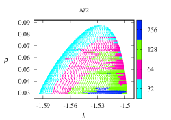
Figure 2. Tori with $\rho>\nu_{v}^{h_{0}}$ of the Lissajous family of the Earth-Moon RTBP around $L_{1}$, computed with the large matrix procedure (left) and the parameterization one (right).

In a second exploration, we have computed invariant tori that are born from planar Lyapunov orbits that have rotation number $\rho<\nu_{v}^{h_{0}}$. Namely, we have chosen 31 values of $\rho$, equally spaced between 0.02785 and 0.00317, nobilized with an absolute tolerance of $1.6\times 10^{-4}$ and for each of the values we have performed continuation of invariant curves given by planar generators $K_{p}$, for constant $\omega=1-1/(1+\rho)$ and increasing $T$, starting from a narrow torus around a planar Lyapunov p.o. The parameters used in the continuation algorithms have been the same as before. The continuations have stopped either by reaching the computational limit or, as in the first exploration, when $|C_{1}(\hat{K})|=|C(K_{v})|<0.001$ (see Section 4.2).

The motivation of this second exploration is twofold. On the one hand, to perform a “stress test” of our procedure by exploring phase space beyond the computations of [27]. On the other, to relate the behavior of dynamical and geometrical observables to the destruction of invariant tori (see the next section). In this exploration, we have always achieved convergence of Newton’s method provided that the continuation step is small enough and the number of points $N$ large enough. The computational limits on these two quantities, chosen as $10^{-5}$ and $8192$, respectively, have been set in order to obtain reasonable run time and storage requirements in a single workstation. Notice that working with such a large number of Fourier coefficients is unfeasible with the large matrix approach, since it would require the solution of non-linear sytems of equations with a size of nearly $100000\times 100000$. A limit, equal to 10000, has also been put for the maximum number of tori computed in each constant $\rho$ family of this second exploration. With all these limits, this exploration has run for a total time of 27.0816 days and has generated a total of $130574$ tori that, each compressed as a bz2 file, take up $127.51\,{\rm GiB}$ of disk space.

The results of this second exploration are shown in Fig. 3, that is analogous to Fig. 2 right but including both explorations. Many of the figures that follow will refer to the two explorations as a whole.

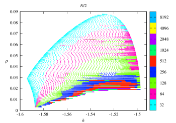
Figure 3. Number of Fourier coefficients of all the tori and invariant bundles computed of the Lissajous family of the Earth-Moon RTBP around $L_{1}$, using this paper’s parameterization strategy.

4.4. Dynamical and geometric observables

In this section we will describe the behaviour of different dynamical and geometric observables of the invariant tori of the Lissajous family that are obtained during their computation. These observables provide insight on both numerical and dynamical vicissitudes faced by the method. We will also display the evolution of three constant $\rho$ families through the 3D representation of some of their tori in configuration space. The results presented here complement those in [27] that, by using iso-energetic Poincaré sections, provides a detailed account of the evolution of the Lissajous family of invariant tori, together with its interaction with other families of invariant tori and periodic orbits.

For a parameterization $K=K_{0}:{\mathbb{T}}\to{\mathbb{R}}^{6}$ of the invariant curve of the time $T$-flow with rotation number $\omega$, obtained with multiple shooting with $m=4$ steps, that is a generator of the 2D invariant torus given by (8), the dynamical observables we consider here are:

• the flying time $T$ of the generator (notice that we get frequencies for the 2D-torus by the formula $\hat{\omega}=\tfrac{1}{T}(\omega,1)$);

• the unstable Floquet multiplier $\Lambda^{u}=\lambda^{-m}$, that provides information about hyperbolity properties of the invariant curve, and from which one can obtain the Floquet exponent of the 2D-torus by $\chi=\tfrac{1}{T}\log\Lambda^{u}$.

Notice we select $m$ so that $\lambda^{-1}$ is not too big, in order to mitigate numerical unstabilities. In our computations, $\lambda^{-1}$ runs in the interval $[4,8]$.

The geometric observables we consider are:

• The Calabi invariants $C_{1}(\hat{K}),C_{2}(\hat{K})$ of the parameterization $\hat{K}(\theta_{1},\theta_{2})$ of the torus with natural frequencies $\hat{\omega}=(\omega_{p},\omega_{v})$. These invariants give insight on the size of the generators in area units. Section 4.2 provides formulae for their computation from $C(\hat{K}_{p})$, $C(\hat{K}_{v})$.

• The (minimum) distances between several pairings of bundles on the generator curve: $T{\mathcal{K}}$, the tangent bundle of the generator curve (generated by $K^{\prime}$); $X$, the bundle generated by the vector field on the curve; the stable and the unstable bundles $E^{s}$ and $E^{u}$, respectively; the central bundle, $E^{c}$, that has rank 4 and contains the tangent bundle to the generator, the vector field and, hence, the tangent bundle to the 2D torus. The distances we consider are: $d(T{\mathcal{K}},X)$, to measure the transversality of the flow to the generator, and $d(E^{s},E^{u})$, $d(E^{s},E^{c})$, and $d(E^{u},E^{c})$, to measure the quality of hyperbolicity geometrical properties.

The bundles are generated by selected columns of the matrix map $P=P_{0}:{\mathbb{T}}\to{\mathbb{R}}^{6\times 6}$, that we write as

$$P(\theta)=\begin{pmatrix}K^{\prime}(\theta)&X_{H}(K(\theta))&W^{s}(\theta)&N^{1}(\theta)&N^{2}(\theta)&W^{u}(\theta)\end{pmatrix}$$

for reference. Hence, at a point $K(\theta)$ of the invariant curve, the fiber of the stable bundle $E^{s}$ is generated by $W^{s}(\theta)$, the fiber of the unstable bundle $E^{u}$ is generated by $W^{u}(\theta)$, and fiber of the center bundle $E^{c}$ is generated by $K^{\prime}(\theta)$, $X_{H}(K(\theta))$, $N^{1}(\theta)$, $N^{2}(\theta)$. Notice that the tangent bundle to the generator is generated by $K^{\prime}(\theta)$, and the tangent bundle of the 2D torus is generated by $K^{\prime}(\theta)$, $X_{H}(K(\theta))$. There are several ways of defining distances or angles between vector subspaces of a given normed vector space. Here, the vector space is ${\mathbb{R}}^{6}$, with the norm induced by the standard scalar product, and the distance we consider between a vector subspace $E_{1}$ of dimension $1$ and another vector subspace $E_{2}$ is the length of the projection onto $E_{2}^{\perp}$ of a unit vector in $E_{1}$ (the angle between $E_{1}$ and $E_{2}$ is the $\arcsin$ of this lenght). Finally, we define the distance between two bundles as the minimum distance between corresponding fibres of the bundles.

Remark 4.4.1.

We emphasize that the quality of hyperbolicity properties of the invariant torus are not only given by the Floquet multipliers in the stable and unstable directions, that have to be away from 1, but also by the positivity of the angles between the stable, unstable and center directions. There are mechanisms of breakdown of invariant tori that involve the degeneration of some of these angles, that go to zero, while the stable and unstable Floquet multipliers remain far from 1. See [10, 11, 12, 23, 30, 33].

Remark 4.4.2.

Reversibility properties of the RTBP imply that stable and unstable bundles can be obtained from each other using reversors, and that they have same angles with the center manifold of the torus. These properties could also be used to reduce the cost of the algorithms presented here (reducing, for instace, the cost of generating the frame). We prefer not doing so for the sake of generality.

By monitoring these observables during the continuation we can get insight about dynamical and geometric properties of the torus (and its invariant bundles), and detect numerical unstabilities caused by degeneracies of these properties (such as the hyperbolicity, regularity of the frame, size of the generator). For instance, we recall that one stopping criterion is that $|C_{1}(\hat{K})|=|C(K_{v})|<0.001$, revealing that the torus is approaching a periodic orbit. We have collected these observables from the two numerical explorations exposed in the previous section, and the results are summarized in Figure 4.

In this massive computation we observe that:

• The unstable multiplier ranges from $413.205$ to $3344.26$, from which the spectral condition of hyperbolicity of the torus is satisfied;

• The distance between the stable and unstable bundles is bigger than 0.492489, and the distante between the stable and center bundle, and the unstable and center bundle, is bigger than 0.0615721, from which the geometrical conditions of hyperbolicy is also satisfied.

The continuations of families of Lissajous tori with smaller rotation numbers stop because of the computational limit of 10000 tori for each constant-$\rho$ family. But, as we see from the behavior of the observables, this phenomenon is not apparently due to the fact that hyperbolicity breaks down. However, the fact that the step size of the continuation becomes smaller and the number of Fourier coefficients becomes larger reveals that the torus is losing regularity (the analyticy strip of the complex domain of the parameterization of the torus goes to zero), indicating an obstruction for the existence of the torus and that it is breaking down. There is another possible mechanism of breakdown, it is what we call KAM breakdown. These tori lie on the center manifold of the $L^{1}$ point, $W^{c}(L_{1})$, which is a $4D$ symplectic manifold. So, inside $W^{c}(L_{1})$, these tori are KAM tori, and the basic mechanism of breakdown is the collision with resonances (the overlap criterion [16]), which can be more geometrically described as the obstruction produced by homoclinic and heteroclinic webs produced by the invariant manifolds of unstable periodic orbits inside the center manifold (the obstruction criterion in [45, 19]). So, it is very likely that in this case the breakdown is produced by this phenomenon inside the center manifold. We will come back to this issue later.

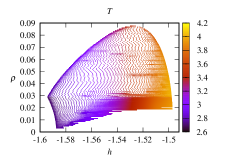
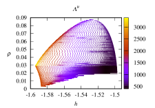
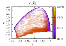
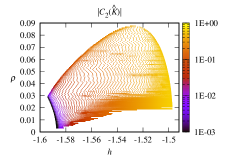
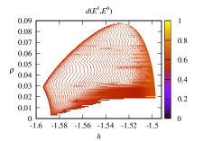
Figure 4. Dynamical and geometrical observables

In the following, we will particularize the results for three families of Lissajous tori, with rotation numbers $\rho=0.031865$, $\rho=0.019091$ and $\rho=0.013584$. Figs. 5, 6 and 7 show several samples of tori of these three families, projected on the configuration space in different forms and views:

• as grids on the parameterized surfaces $\{\hat{K}(\theta_{1},\theta_{2})\}_{(\theta_{1},\theta_{2})\in{\mathbb{T}}^{2}}$ (see Eq. (8)), including two generators of the homothopy group of the torus, given by $\{\hat{K}(\theta,0)\}_{\theta\in{\mathbb{T}}}$, in blue, and $\{\hat{K}(0,\theta)\}_{\theta\in{\mathbb{T}}}$, in red;

• as opaque surfaces, with the same scale and range on all axes, with colors corresponding to the different sides of the surface, revealing self-intersections of the projections of tori on configuration space.

Actually, instead of Eq. (8), the expression

$$\hat{K}(\theta_{1},\theta_{2})=\varphi_{(\theta_{2}-\frac{j}{m})T}\Bigl{(}K_{j}\bigl{(}\theta_{1}-(\theta_{2}-\frac{j}{m})\omega\bigr{)}\Bigr{)},$$

with $j=[m\theta_{2}]$, has been used, in order to take advantage of multiple shooting. In addition to these views, for each of these families we have plotted in Figs. 9, 10 and 11 the dynamical and geometrical observables as functions of the energy $h$. We will describe our findings below.

The results for the family $\rho=0.031865$ are summarized in Figs. 5 and 9. From Fig. 5 we appreciate how the family begins with a small torus around a vertical Lyapunov p.o., that grows up to approximately the size of the planar Lyapunov orbit of the same energy, and then starts bending until it “is about to close”. Then it opens again and shrinks until it collapses to a vertical Lyapunov p.o. of higher energy. All this is done while increasing in size, since energy also increases. Fig. 9 displays the observables for this family. Since the family is born in a vertical Lyapunov p.o. and dies in another vertical Lyapunov p.o. of a higher energy, the Calabi invariant of the generator starts being 0 and finishes being 0. Notice that, in both cases, close to the p.o. the Calabi invariant goes to zero assymptotically as a linear function of the difference of the energy with the one of the p.o.

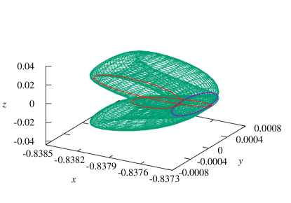
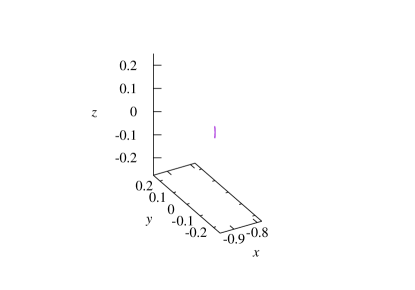
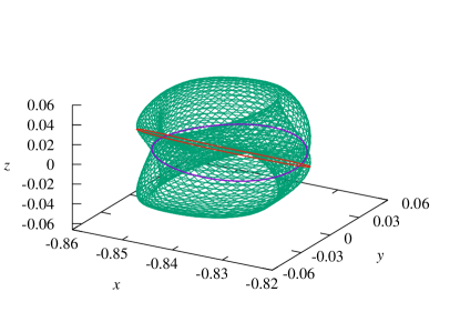
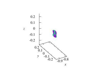
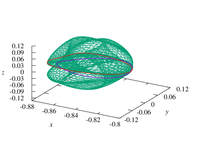
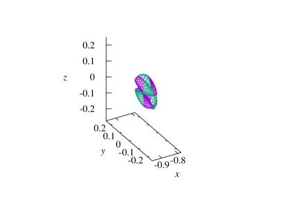
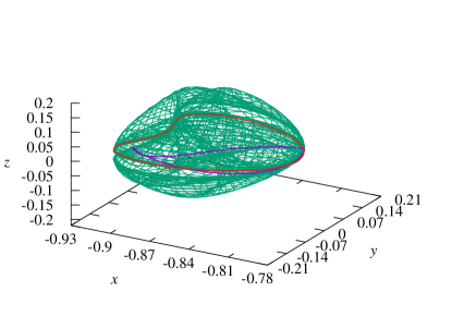
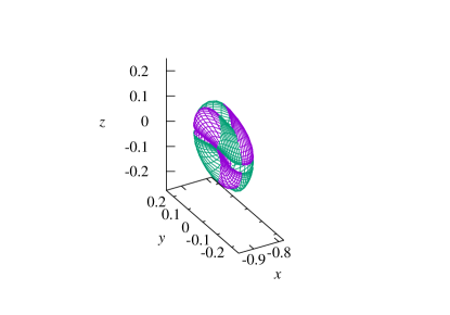
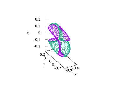
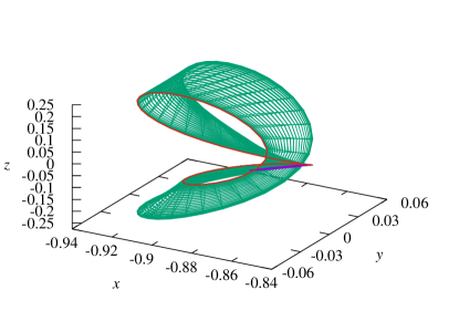
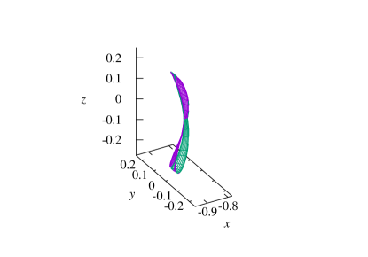
Figure 5. Two views of a sample of invariant tori with $\rho=0.031865$. Letf: Parameterized surfaces, including generators (Blue: invariant curve $\{\hat{K}(\theta,0)\}_{\theta\in{\mathbb{T}}}$. Red: invariant curve $\{\hat{K}(0,\theta)\}_{\theta\in{\mathbb{T}}}$). Right: with the same scale on all axes, and with opaque surfaces.

The results for the family $\rho=0.019091$ are summarized in Figs. 6 and 10. Fig. 6 shows a sample tori starting in a planar Lyapunov p.o. and, hence, their homothopy group generators are exchanged with respect to Fig. 5. The evolution with energy is similar to the one of Fig. 6, with three main differences: the torus “seems to close after bending” (a zoom of the fourth torus reveals that it does not actually close), there is a more important accumulation of wireframe lines at the “boundary that closes and opens”, and the family starts from a planar Lyapunov p.o. instead of a vertical one. This is in fact the reason the Calabi invariant of the computed generators starts being 0 (and, again, with an asymptotic linear behaviour) and increases till the end of the continuation (converging to the Calabi invariant of the vertical Lyapunov p.o.), as it is observed in Fig. 10.

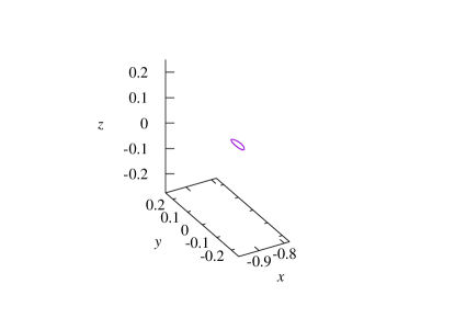
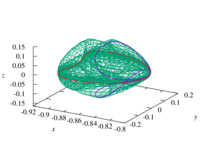
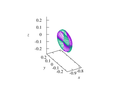
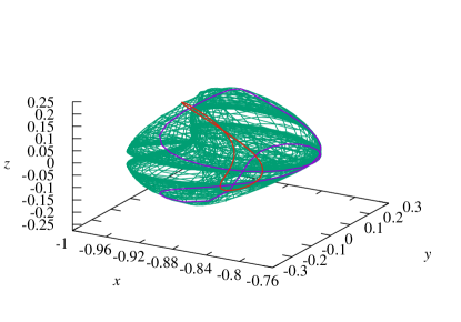
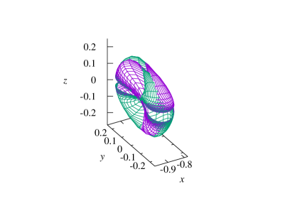
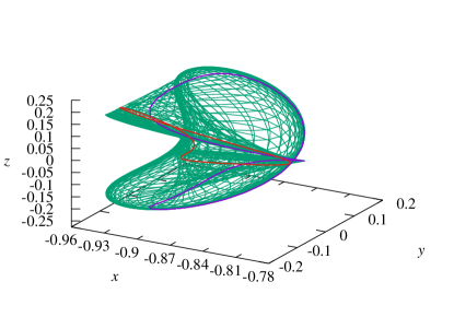
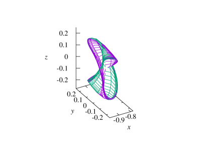
Figure 6. Two views of a sample of invariant tori with $\rho=0.019091$. Left: parameterized surfaces, including generators (Blue: invariant curve $\{\hat{K}(\theta,0)\}_{\theta\in{\mathbb{T}}}$. Red: invariant curve $\{\hat{K}(0,\theta)\}_{\theta\in{\mathbb{T}}}$). Right: with the same scale on all axes, and with opaque surfaces.

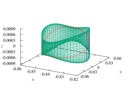
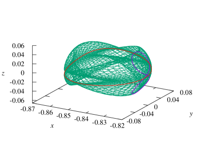
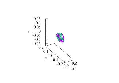
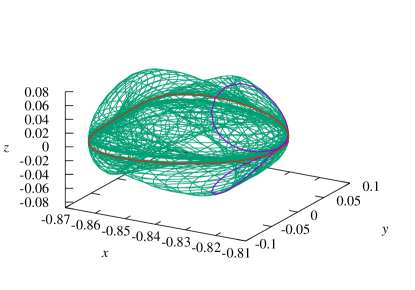
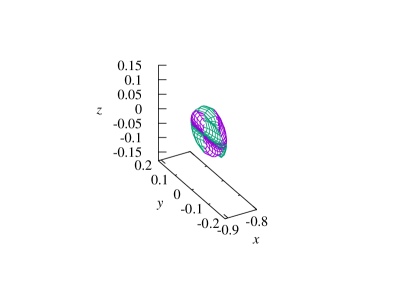
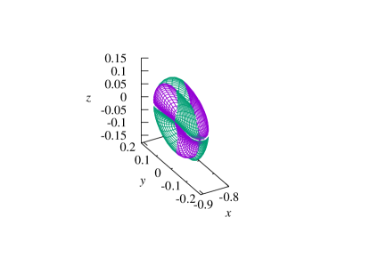
Figure 7. Two views of a sample of invariant tori with $\rho=0.013584$. Left: parameterized surfaces, including generators (Blue: invariant curve $\{\hat{K}(\theta,0)\}_{\theta\in{\mathbb{T}}}$. Red: invariant curve $\{\hat{K}(0,\theta)\}_{\theta\in{\mathbb{T}}}$). Right: with the same scale on all axes, and with opaque surfaces.

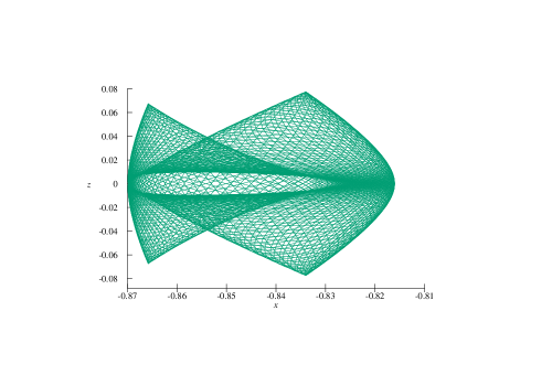
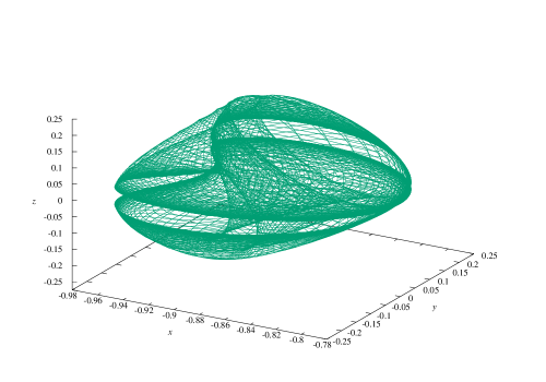
Figure 8. Magnifications of projections of the third and fifth tori of Fig. 6, corresponding to $\rho=0.019091$.

In the iso-energetic Poincaré section plots of [27] (and, for lower energy levels, in the ones of previous references like [26, 41]), it is numerically seen that, from energy $h_{B}$ to $h_{C}$, a double homoclinic connection inside $W^{c}(L_{1})$ of the planar Lyapunov family of p.o. acts as separatrix from the Lissajous family and the quasi-Halo family of tori. From energy $h_{C}$ to $h_{D}$, this role is taken by heteroclinic connections (also inside $W^{c}(L_{1})$) between the vertically symmetric families of p.o. that are born at the second 1:1 bifurcation of the planar Lyapunov p.o. Plots of orbits of these last families of p.o. can be found in Fig. 8 of [27] (they are known as “axial” by other autors, e.g. [20]). In Fig. 6, it is observed how the tori approach these connections. This fact is better appreciated in Fig. 8, that shows magnifications of projections of the third and fifth tori of Fig. 6. The view of the third torus has been chosen in order to stress the fact that the torus represented approaches two different, vertically simmetric quasi-Halo tori, as can be inferred from the Poincaré representations of the center manifold in references [27, 26, 41]. When approaching these connections, dynamics becomes slow and, since the parameterization $\hat{K}$ is tied to the dynamics through the invariance equation (5), it produces the accumulation of wireframe lines of Fig. 6 and the small values of $d(T{\mathcal{K}},X)$ of Fig. 4. We believe this kind of stiffness to be responsible for the drastic reduction of step length of the second exploration and, to a lesser extent, of the first one. As it has been commented, these connections are responsible for the destruction of the families of invariant tori in the center manifold.

The phenomenon of breakdown is illustrated with the family with $\rho=0.013584$. The results for this family are summarized in Figs. 7 and 11. In Fig. 7 we observe that the torus is increasingly pinched, while dynamical and geometrical observables in Fig. 11 do not suggest the torus is being destroyed. However, the fact the continuation step is getting very small and the number of Fourier coefficients of the approximations is getting larger, related to the mentioned “pinching phenomenon”, envisages the breakdown of the torus inside the center manifold.

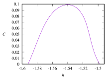
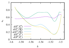
Figure 9. Calabi invariant $C(K_{v})=C_{1}(\hat{K})$, and distances between several pairings of bundles, for the family $\rho=0.031865$.

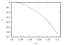
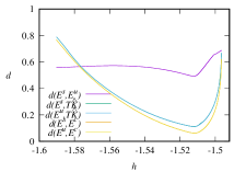
Figure 10. Calabi invariant $C(K_{p})=-C_{2}(\hat{K})$, and distances between several pairings of bundles, for the family $\rho=0.019091$.

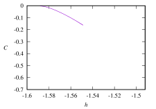
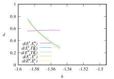
Figure 11. Calabi invariant $C(K_{p})=-C_{2}(\hat{K})$, and distances between several pairings of bundles, for the family $\rho=0.013584$.

5. Conclusion

We have presented in this paper a very efficient method to compute invariant tori in Hamiltonian systems. To do so, we have first reduced the dimensionaly of the objects, by considering invariant tori for flow maps, and then taken advantage of the geometrical and dynamical properties of invariant tori in Hamiltonian systems. The method also provides online information on the linearized dynamics around the torus, as well as on other geometrical properties. He have focused our attention on partially hyperbolic invariant tori with rank-one stable and unstable manifolds, and in this case the method provides not only parameterizations of the tori but also of the linear approximations of those manifolds. Tests have been performed for the computation of invariant tori around libration points of the Circular Restricted Three Body Problem, for which there is an extensive literature, so any one could easily compare the performances.

As we have already mentioned, we only present algorithms of computation, based on Newton’s method. Eventually, a proof of convergence could be completed using KAM techniques for obtaining results in a posteriori format. Although we have not attempted this, we do provide information about the magical cancellations appearing in the linearized equations, that are key in the KAM proofs, and, with much more effort, could be implemented as computer assisted proofs [22].

The increasing complexity of problems and applications has spurred the research of this paper. The algorithms presented here are the first ones in a new generation of algorithms to compute invariant tori and their manifolds in Hamiltonian systems. We plan to extend the methodologies to more complex problems in the future, with an eye in the applications.

Appendix A From Poincaré map to time-$T$ map

In this section we will see how to obtain, from an invariant torus of a the Poincaré map, an invariant torus of a time-$T$ map. For instance, the invariant torus of the Poincaré map could have been computed from a center manifold reduction around an equilibrium point at a certain fixed energy level (see e.g. [49, 38] for normal form methods and [29] for direct parameterization methods, applied to the computation of the center manifold of a colinear fixed point in the RTBP).

Assume we are given a parameterization $K_{P}:{\mathbb{T}}^{d-1}\to{\mathbb{R}}^{2n}$ of a $(d-1)$-dimensional torus ${\mathcal{K}}_{P}$ inside a $d$-dimensional torus $\hat{\mathcal{K}}$, produced by a Poincaré map $P$ associated to a transversal section to the vector field $X_{H}$. We also assume that the rotation vector of ${\mathcal{K}}_{P}$ is $\omega$ (which is assumed to be Diophantine). That is, we assume for all $\theta\in{\mathbb{T}}^{d-1}$

$$\varphi_{T_{P}(\theta)}(K_{P}(\theta))=K_{P}(\theta+\omega),$$

where $T_{P}:{\mathbb{T}}^{d-1}\to{\mathbb{R}}$ gives for each $\theta\in{\mathbb{T}}^{d-1}$ the time for a point $K_{P}(\theta)$ to return to the transversal section. The flying time depends then on the point on the torus.

We want to find a parameterization $K:{\mathbb{T}}^{d-1}\to{\mathbb{R}}^{2n}$ of a $(d-1)$-dimensional torus ${\mathcal{K}}$ for which the flying time is constant. To do so, we look for $\tau:{\mathbb{T}}^{d-1}\to{\mathbb{R}}$ and $T$ such that

$$K(\theta)=\varphi_{\tau(\theta)}(K_{P}(\theta)),\ \varphi_{T}(K(\theta))=K(\theta+\omega).$$

Hence, since

$$\varphi_{T}(K(\theta))=\varphi_{T+\tau(\theta)}(K_{P}(\theta))$$

and

$$K(\theta+\omega)=\varphi_{\tau(\theta+\omega)}(K_{P}(\theta+\omega))=\varphi_{\tau(\theta+\omega)+T_{P}(\theta)}(K_{P}(\theta)),$$

we impose that

$$\tau(\theta)-\tau(\theta+\omega)=T_{P}(\theta)-T.$$

This is the well-known small divisors equation (discussed here in Section 3.2). We adjust then $T$ to be the average of $T_{P}$, $T=\langle T_{P}\rangle$, and solve for $\tau$. Notice that $\tau$ is defined up to a constant, the average that we take as $0$. This is natural since $K$ is determined up to a time translation (see Remark 2.4.3).

Appendix B Quadratically small averages

In this section we will prove that, given a multiple torus $\{K_{i}(\theta)\}_{i=0}^{m-1}$, approximately invariant with errors

$$E_{i}(\theta)=\varphi_{T/m}(K_{i}(\theta))-K_{i+1}(\theta+\tfrac{\omega}{m}),$$

then the averages of $\{\eta_{i}^{3}(\theta)\}_{i=0}^{m-1}$ given by

$$\eta_{i}^{3}(\theta)=\begin{pmatrix}-{\rm D}K_{i+1}(\theta+\tfrac{\omega}{m})^{\top}\Omega(K_{i+1}(\theta+\tfrac{\omega}{m}))E_{i}(\theta)\\ -X_{H}(K_{i+1}(\theta+\tfrac{\omega}{m}))\Omega(K_{i+1}(\theta+\tfrac{\omega}{m}))E_{i}(\theta)\end{pmatrix}=:\begin{pmatrix}\eta_{i}^{31}(\theta)\\ \eta_{i}^{32}(\theta)\end{pmatrix}$$

are quadratically small with respect to the errors (and their derivatives). This is a crucial step in our algorithms, and also in a eventual proof of their convergence using KAM methods.

First, we start by proving that $\langle{\eta}^{32}\rangle$ is quadratically small. In fact

$$\begin{split}\sum_{i=0}^{m-1}\langle\eta_{i}^{32}(\theta)\rangle=&\sum_{i=0}^{m-1}\langle{\rm D}H(K_{i+1}(\theta+\tfrac{\omega}{m}))E_{i}(\theta)\rangle\\ =&\sum_{i=0}^{m-1}\langle H(\varphi_{T/m}(K_{i}(\theta))-H(K_{i+1}(\theta+\tfrac{\omega}{m}))\rangle\\ &-\sum_{i=0}^{m-1}\langle\int_{0}^{1}(1-s)\ {\rm D}^{2}H(K_{i+1}(\theta+\tfrac{\omega}{m})+sE_{i}(\theta))[E_{i}(\theta),E_{i}(\theta)]\ ds\rangle\\ =&-\sum_{i=0}^{m-1}\langle\int_{0}^{1}(1-s)\ {\rm D}^{2}H(K_{i+1}(\theta+\tfrac{\omega}{m})+sE_{i}(\theta))[E_{i}(\theta),E_{i}(\theta)]\ ds\rangle,\end{split}$$

which is quadratically small in the errors.

Second, we prove that $\langle{\eta}^{31}\rangle$ is quadratically small. We start using the exactness of the symplectic form:

$$\begin{split}\sum_{i=0}^{m-1}\langle\eta_{i}^{31}(\theta)\rangle=&-\sum_{i=0}^{m-1}\langle{\rm D}K_{i+1}(\theta+\tfrac{\omega}{m})^{\top}{\rm D}a(K_{i+1}(\theta+\tfrac{\omega}{m}))^{\top}E_{i}(\theta)\rangle\\ &+\sum_{i=0}^{m-1}\langle{\rm D}K_{i+1}(\theta+\tfrac{\omega}{m})^{\top}{\rm D}a(K_{i+1}(\theta+\tfrac{\omega}{m}))E_{i}(\theta)\rangle\\ =&\sum_{i=0}^{m-1}\langle{\rm D}E_{i}(\theta)^{\top}a(K_{i+1}(\theta+\tfrac{\omega}{m}))+{\rm D}K_{i+1}(\theta+\tfrac{\omega}{m})^{\top}(\Delta^{1}a_{i}(\theta)-\Delta^{2}a_{i}(\theta))\rangle,\end{split}$$

where we use

$$\begin{split}0=&\langle{\rm D}\bigl{(}a(K_{i+1}(\theta+\tfrac{\omega}{m}))^{\top}E_{i}(\theta)\bigr{)}\rangle\\ =&\langle E_{i}(\theta)^{\top}{\rm D}(a(K_{i+1}(\theta+\tfrac{\omega}{m})))+a(K_{i+1}(\theta+\tfrac{\omega}{m}))^{\top}{\rm D}E_{i}(\theta)\rangle,\end{split}$$

and the definitions

$$\begin{split}\Delta^{1}a_{i}(\theta)=&a(\varphi_{T/m}(K_{i}(\theta)))-a(K_{i+1}(\theta+\tfrac{\omega}{m}))\\ =&\int_{0}^{1}{\rm D}a(K_{i+1}(\theta+\tfrac{\omega}{m})+sE_{i}(\theta))E_{i}(\theta)\ ds\end{split}$$

and

$$\begin{split}\Delta^{2}a_{i}(\theta)=&a(\varphi_{T/m}(K_{i}(\theta)))-a(K_{i+1}(\theta+\tfrac{\omega}{m}))-{\rm D}a(K_{i+1}(\theta+\tfrac{\omega}{m}))E_{i}(\theta)\\ =&\int_{0}^{1}(1-s)\ {\rm D}^{2}a(K_{i+1}(\theta+\tfrac{\omega}{m})+sE_{i}(\theta))[E_{i}(\theta),E_{i}(\theta)]\ ds.\end{split}$$

Hence, using that

$${\rm D}\varphi_{T/m}(K_{i}(\theta)){\rm D}K_{i}(\theta)-{\rm D}K_{i+1}(\theta+\tfrac{\omega}{m})={\rm D}E_{i}(\theta)$$

and that

$$\sum_{i=0}^{m-1}\langle{\rm D}K_{i+1}(\theta+\tfrac{\omega}{m})^{\top}a(K_{i+1}(\theta+\tfrac{\omega}{m}))\rangle=\sum_{i=0}^{m-1}\langle{\rm D}K_{i}(\theta)^{\top}a(K_{i}(\theta))\rangle$$

we have:

$$\begin{split}\sum_{i=0}^{m-1}\langle\eta_{i}^{31}(\theta)\rangle=&\phantom{+}\sum_{i=0}^{m-1}\langle{\rm D}K_{i}(\theta)^{\top}\bigl{(}{\rm D}\varphi_{T/m}(K_{i}(\theta))^{\top}a(\varphi_{T/m}(K_{i}(\theta)))-a(K_{i}(\theta))\bigr{)}\rangle\\ &-\sum_{i=0}^{m-1}\langle{\rm D}E_{i}(\theta)^{\top}\Delta^{1}a_{i}(\theta)+{\rm D}K_{i+1}(\theta+\tfrac{\omega}{m})^{\top}\Delta^{2}a_{i}(\theta)\rangle\\ =&\phantom{+}\sum_{i=0}^{m-1}\langle{\rm D}\bigl{(}p_{T/m}(K_{i}(\theta))\bigr{)}^{\top}\rangle\\ &-\sum_{i=0}^{m-1}\langle{\rm D}E_{i}(\theta)^{\top}\Delta^{1}a_{i}(\theta)+{\rm D}K_{i+1}(\theta+\tfrac{\omega}{m})^{\top}\Delta^{2}a_{i}(\theta)\rangle\\ =&-\sum_{i=0}^{m-1}\langle{\rm D}E_{i}(\theta)^{\top}\Delta^{1}a_{i}(\theta)+{\rm D}K_{i+1}(\theta+\tfrac{\omega}{m})^{\top}\Delta^{2}a_{i}(\theta)\rangle,\end{split}$$

which is quadratically small. We have used the exactness of the Hamiltonian flow, being $p_{t}$ is the primitive function of $\varphi_{t}$.

References

- [1] R.A. Adomaitis, I.G. Kevrekidis, and R. de la Llave. A computer-assisted study of global dynamic transitions for a noninvertible system. Internat. J. Bifur. Chaos Appl. Sci. Engrg., 17(4):1305–1321, 2007.
- [2] Eugene L. Allgower and Kurt Georg. Numerical continuation methods, volume 13 of Springer Series in Computational Mathematics. Springer-Verlag, Berlin, 1990. An introduction.
- [3] Nicola Baresi, Zubin P. Olikara, and Daniel J. Scheeres. Fully numerical methods for continuing families of quasi-periodic invariant tori in astrodynamics. The Journal of the Astronautical Sciences, 2018.
- [4] E. Oran Brigham. The Fast Fourier Transform and its applications. Prentice–Hall, 1988.
- [5] X. Cabré, E. Fontich, and R. de la Llave. The parameterization method for invariant manifolds. I. Manifolds associated to non-resonant subspaces. Indiana Univ. Math. J., 52(2):283–328, 2003.
- [6] X. Cabré, E. Fontich, and R. de la Llave. The parameterization method for invariant manifolds. II. Regularity with respect to parameters. Indiana Univ. Math. J., 52(2):329–360, 2003.
- [7] X. Cabré, E. Fontich, and R. de la Llave. The parameterization method for invariant manifolds. III. Overview and applications. J. Differential Equations, 218(2):444–515, 2005.
- [8] R. Calleja, A. Celletti, and R. de la Llave. A KAM theory for conformally symplectic systems: efficient algorithms and their validation. J. Differential Equations, 255(5):978–1049, 2013.
- [9] R. Calleja and R. de la Llave. Fast numerical computation of quasi-periodic equilibrium states in 1D statistical mechanics, including twist maps. Nonlinearity, 22(6):1311–1336, 2009.
- [10] R. Calleja and J.-Ll. Figueras. Collision of invariant bundles of quasi-periodic attractors in the dissipative standard map. Chaos: An Interdisciplinary Journal of Nonlinear Science, 22(3):033114, 2012.
- [11] M. Canadell and A. Haro. Parameterization method for computing quasi-periodic reducible normally hyperbolic invariant tori. In F. Casas, V. Martínez (eds.), Advances in Differential Equations and Applications, volume 4 of SEMA SIMAI Springer Series. Springer, 2014.
- [12] M. Canadell and À. Haro. Computation of Quasi-Periodic Normally Hyperbolic Invariant Tori: Algorithms, Numerical Explorations and Mechanisms of Breakdown. J. Nonlinear Sci., 27(6):1829–1868, 2017.
- [13] M. Canadell and À. Haro. Computation of Quasiperiodic Normally Hyperbolic Invariant Tori: Rigorous Results. J. Nonlinear Sci., 27(6):1869–1904, 2017.
- [14] Enric Castellà and Àngel Jorba. On the vertical families of two-dimensional tori near the triangular points of the bicircular problem. Celestial Mech. Dynam. Astronom., 76(1):35–54, 2000.
- [15] T.N. Chan. Numerical Bifurcation Analysis of Simple Dynamical Systems. PhD thesis, Concordia University, Montreal, Canada, September 1983.
- [16] B.V. Chirikov. A universal instability of many-dimensional oscillator systems. Phys. Rep., 52(5):264–379, 1979.
- [17] R. de la Llave. A tutorial on KAM theory. In Smooth ergodic theory and its applications (Seattle, WA, 1999), volume 69 of Proc. Sympos. Pure Math., pages 175–292. Amer. Math. Soc., Providence, RI, 2001.
- [18] R. de la Llave, A. González, À. Jorba, and J. Villanueva. KAM theory without action-angle variables. Nonlinearity, 18(2):855–895, 2005.
- [19] R. de la Llave and A. Olvera. The obstruction criterion for non-existence of invarian circles and renormalization. Nonlinearity, 19(8):1907–1937, 2006.
- [20] D.J. Dichmann, E.J. Doedel, and R.C. Paffenroth. The computation of periodic solutions of the 3-body problem using the numerical continuation software AUTO. In G. Gómez, M. W. Lo, and J. J. Masdemont, editors, Libration Point Orbits and Applications. World Scientific, 2003.
- [21] D. W. Dunham and R. W. Farquhar. Libration point missions, 1978–2002. In G. Gómez, M. W. Lo, and J. J. Masdemont, editors, Libration Point Orbits and Applications, Singapore, 2003. World Scientific. Proceedings of the conference Libration Point Orbits and Applications, Aiguablava (Girona, Spain), June 10–14, 2002.
- [22] J.-Ll. Figueras, A. Haro, and A. Luque. Rigorous Computer-Assisted Application of KAM Theory: A Modern Approach. Found. Comput. Math., 17(5):1123–1193, 2017.
- [23] Jordi-Lluís Figueras and Àlex Haro. Different scenarios for hyperbolicity breakdown in quasiperiodic area preserving twist maps. Chaos, 25(12):123119, 16, 2015.
- [24] E. Fontich, R. de la Llave, and Y. Sire. Construction of invariant whiskered tori by a parameterization method. I. Maps and flows in finite dimensions. J. Differential Equations, 246(8):3136–3213, 2009.
- [25] C. Gasquet and P. Witomski. Fourier analysis and applications, volume 30 of Texts in Applied Mathematics. Springer-Verlag, New York, 1999. Filtering, numerical computation, wavelets, Translated from the French and with a preface by R. Ryan.
- [26] G. Gómez, À. Jorba, C. Simó, and J. Masdemont. Dynamics and mission design near libration points. Vol. III, volume 4 of World Scientific Monograph Series in Mathematics. World Scientific Publishing Co. Inc., River Edge, NJ, 2001. Advanced methods for collinear points.
- [27] G. Gómez and J.M. Mondelo. The dynamics around the collinear equilibrium points of the RTBP. Phys. D, 157(4):283–321, 2001.
- [28] A. González, A. Haro, and R. de la Llave. Singularity theory for non-twist KAM tori. Mem. Amer. Math. Soc., 227(1067):vi+115, 2014.
- [29] À. Haro, M. Canadell, J.-Ll. Figueras, A. Luque, and J.-M. Mondelo. The parameterization method for invariant manifolds, volume 195 of Applied Mathematical Sciences. Springer, [Cham], 2016. From rigorous results to effective computations.
- [30] A. Haro and R. de la Llave. Manifolds on the verge of a hyperbolicity breakdown. Chaos, 16(1):013120, 8, 2006.
- [31] A. Haro and R. de la Llave. A parameterization method for the computation of invariant tori and their whiskers in quasi-periodic maps: numerical algorithms. Discrete Contin. Dyn. Syst. Ser. B, 6(6):1261–1300, 2006.
- [32] A. Haro and R. de la Llave. A parameterization method for the computation of invariant tori and their whiskers in quasi-periodic maps: rigorous results. J. Differential Equations, 228(2):530–579, 2006.
- [33] A. Haro and R. de la Llave. A parameterization method for the computation of invariant tori and their whiskers in quasi-periodic maps: explorations and mechanisms for the breakdown of hyperbolicity. SIAM J. Appl. Dyn. Syst., 6(1):142–207 (electronic), 2007.
- [34] Peter Henrici. Fast fourier methods in computational complex analysis. SIAM Review, 21(4):481–527, 1979.
- [35] M. Huang, T. Küpper, and N. Masbaum. Computation of invariant tori by the Fourier methods. SIAM J. Sci. Comput., 18(3):918–942, 1997.
- [36] G. Huguet. The role of hyperbolic invariant objects: from Arnold difussion to biological clocks. PhD thesis, Departament de Matemàtica Aplicada I, Universitat Politècnica de Catalunya, 2008. http://www.ma.utexas.edu/users/ghuguet/tesi/.
- [37] G. Huguet, R. de la Llave, and Y. Sire. Computation of whiskered invariant tori and their associated manifolds: new fast algorithms. Discrete Contin. Dyn. Syst., 32(4):1309–1353, 2012.
- [38] À. Jorba. A methodology for the numerical computation of normal forms, centre manifolds and first integrals of Hamiltonian systems. Experiment. Math., 8(2):155–195, 1999.
- [39] À. Jorba and E. Olmedo. On the computation of reducible invariant tori on a parallel computer. SIAM J. Appl. Dyn. Syst., 8(4):1382–1404, 2009.
- [40] Àngel Jorba. Numerical computation of the normal behaviour of invariant curves of -dimensional maps. Nonlinearity, 14(5):943–976, 2001.
- [41] Àngel Jorba and Josep J. Masdemont. Dynamics in the center manifold of the Restricted Three–Body Problem. Physica D, 132:189–213, 1999.
- [42] A. Luque and J. Villanueva. A KAM theorem without action-angle variables for elliptic lower dimensional tori. Nonlinearity, 24(4):1033–1080, 2011.
- [43] K. R. Meyer, G. R. Hall, and D. Offin. Introduction to Hamiltonian Dynamical Systems and the –Body Problem. Springer–Verlag, 2nd edition, 2009.
- [44] J.-M. Mondelo, E. Barrrabés, G. Gómez, and M. Ollé. Fast numerical computation of Lissajous and quasi–halo libration point trajectories and their invariant manifolds. Paper IAC-12,C1,6,9,x14982. Proceedings of the 63rd International Astronautical Congress, 1-5 October 2012, Naples, Italy.
- [45] A. Olvera and C. Simó. An obstruction method for the destruction of invariant curves. Phys. D, 26(1-3):181–192, 1987.
- [46] W. H. Press, S. A. Teukolsky, W. T. Vetterling, and B. P. Flannery. Numerical Recipes in C++: The Art of Scientific Computing. Cambridge University Press, 2nd edition, 2002.
- [47] F. Schilder, W. Vogt, S. Schreiber, and H.M. Osinga. Fourier methods for quasi-periodic oscillations. Internat. J. Numer. Methods Engrg., 67(5):629–671, 2006.
- [48] C. L. Siegel and J. K. Moser. Lectures on celestial mechanics. Classics in Mathematics. Springer-Verlag, Berlin, 1995. Translated from the German by C. I. Kalme, Reprint of the 1971 translation.
- [49] C. Simó. Effective computations in celestial mechanics and astrodynamics. In Modern methods of analytical mechanics and their applications (Udine, 1997), volume 387 of CISM Courses and Lectures, pages 55–102. Springer, Vienna, 1998.
- [50] J. Stoer and R. Bulirsch. Introduction to numerical analysis. Springer, Berlin, second edition, 1993.
- [51] Victor Szebehely. Theory of orbits. The Restricted Problem of Three Bodies. Academic Press, 1967.
- [52] Robert L. Warnock. Close approximations to invariant tori in nonlinear mechanics. Phys. Rev. Lett., 66(14):1803–1806, 1991.