Application of the Argument Principle to Functions Expressed as Mellin Transforms

Bjoern S. Schmekel 111bss28@cornell.edu
Department of Physics, College of Studies for Foreign Diploma
Recipients at the University of Hamburg, 20355 Hamburg, Germany
(January 15, 2021)
Abstract

We describe a numerical algorithm for evaluating the numbers of roots minus the number of poles contained in a region based on the argument principle with the function of interest being written as a Mellin transformation of a usually simpler function. Because the function to be transformed may be simpler than its Mellin transform whose roots are to be sought we express the final integrals in terms of the former accepting higher dimensional integrals. Nonlinear terms are expressed as convolutions approximating reciprocal values by exponential sums. As an example the final expression is applied to the Riemann Zeta function. The procedure is very inefficient numerically. However, depending on the function to be investigated it may be possible to find analytical estimates of the resulting integrals.

Keywordsโ€” Root-Finding Algorithms, Argument Principle, Mellin Transformation, Riemann Zeta Function

1 Introduction

Object of this paper is to compute the number of roots minus the number of poles enclosed by a closed contour $C$ using the argument principle

NRโˆ’NP=12โ€‹ฯ€โ€‹iโ€‹โˆฎCfโ€ฒโ€‹(s)fโ€‹(s)โ€‹๐‘‘ssubscript๐‘๐‘…subscript๐‘๐‘ƒ12๐œ‹๐‘–subscriptcontour-integral๐ถsuperscript๐‘“โ€ฒ๐‘ ๐‘“๐‘ differential-d๐‘ \displaystyle N_{R}-N_{P}=\frac{1}{2\pi i}\oint_{C}\frac{f^{\prime}(s)}{f(s)}ds (1.1)

where $f(z)$ is a meromorphic function on and inside of the contour $C$ which can be represented as an auxilliary function multiplied by the Mellin transform of another function

fโ€‹(s)=Kโ€‹(s)โ€‹Zโ€‹(s)=Kโ€‹(s)โ€‹โˆซ0โˆžzโ€‹(t)โ€‹tsโˆ’1โ€‹๐‘‘t๐‘“๐‘ ๐พ๐‘ ๐‘๐‘ ๐พ๐‘ superscriptsubscript0๐‘ง๐‘กsuperscript๐‘ก๐‘ 1differential-d๐‘ก\displaystyle f(s)=K(s)Z(s)=K(s)\int_{0}^{\infty}z(t)t^{s-1}dt (1.2)

assuming the Melling transform exists on and inside of the contour $C$. The latter is chosen such that it does not run over any poles or roots. We are interested in cases where $z(t)$ is a simple function therefore expressing the final result in terms of Kโ€‹(s)๐พ๐‘ K(s) as well as $z(t)$ instead of Zโ€‹(s)๐‘๐‘ Z(s). Furthermore, we are looking for an expression such that eqn. 1.1 can be expressed as a multi-dimensional integral of $z(t)$. Obviously, the integrand in eqn. 1.1 is a nonlinear functional of $z(t)$ (and Kโ€‹(s)๐พ๐‘ K(s) ), so arriving at such a result is not completely straightforward. In a first step we deal with the nonlinearities by approximating the reciprocal value of fโ€‹(s)๐‘“๐‘ f(s) in the argument principle by an exponential sum [1, 2, 3, 4], i.e.

$\displaystyle\frac{1}{x}\approx\sum_{j=1}^{N}\alpha_{j}e^{-c_{j}x}\equiv\mathcal{I}_{1}(x)$ (1.3)

which is possible for $\Re(x)>0$. We will have to ensure this condition is always met possibly adding a factor which changes sign when appropriate.

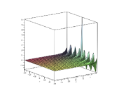
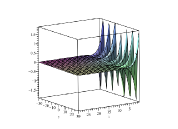
The exponential sum approximation has not been investigated too thoroughly for complex denominators. In fig. 1 The approximation breaks down for small values of $\Re(x)$ as expected, but accuracy is not impacted by an imaginary part as only $\Re(x)>0$ is needed for convergence.

Refer to caption
Refer to caption
Figure 1: Real (above) and imaginary part (below) of the difference of $1/z$ and its exponential sum approximation with $z=x+iy$

Using the following complex sign function

csgn(s)={โˆ’1โ„œโก(s)<01โ„œโก(s)>0sgn(โ„‘โก(s))โ„œโก(s)=0csgn๐‘ cases1๐‘ 01๐‘ 0sgn๐‘ ๐‘ 0\displaystyle\mathop{\rm csgn}(s)=\begin{cases}-1&\Re(s)<0\\ 1&\Re(s)>0\\ \mathop{\rm sgn}\left(\Im(s)\right)&\Re(s)=0\end{cases} (1.4)

and expanding the exponential function as a power series we obtain

$\displaystyle N_{R}-N_{P}$ $\displaystyle=$ 12โ€‹ฯ€โ€‹iโ€‹โˆฎC๐‘‘sโ€‹[Kโ€ฒโ€‹(s)โ€‹Zโ€‹(s)+Kโ€‹(s)โ€‹Zโ€ฒโ€‹(s)]โ€‹โˆ‘j=1Nโˆ‘k=0nฮฑjโ€‹csgn(fโ€‹(s))โ€‹(โˆ’1)kk!โ€‹cjkโ€‹Kkโ€‹(s)โ€‹Zkโ€‹(s)โ€‹csgnk(fโ€‹(s))12๐œ‹๐‘–subscriptcontour-integral๐ถdifferential-d๐‘ delimited-[]superscript๐พโ€ฒ๐‘ ๐‘๐‘ ๐พ๐‘ superscript๐‘โ€ฒ๐‘ superscriptsubscript๐‘—1๐‘superscriptsubscript๐‘˜0๐‘›subscript๐›ผ๐‘—csgn๐‘“๐‘ superscript1๐‘˜๐‘˜superscriptsubscript๐‘๐‘—๐‘˜superscript๐พ๐‘˜๐‘ superscript๐‘๐‘˜๐‘ superscriptcsgn๐‘˜๐‘“๐‘ \displaystyle\frac{1}{2\pi i}\oint_{C}ds\left[K^{\prime}(s)Z(s)+K(s)Z^{\prime}(s)\right]\sum_{j=1}^{N}\sum_{k=0}^{n}\alpha_{j}\mathop{\rm csgn}\left(f(s)\right)\frac{(-1)^{k}}{k!}c_{j}^{k}K^{k}(s)Z^{k}(s){\mathop{\rm csgn}}^{k}\left(f(s)\right) (1.5)
$\displaystyle=$ 12โ€‹ฯ€โ€‹iโ€‹โˆ‘j=1Nโˆ‘k=0nโˆฎC๐‘‘sโ€‹ฮฑjโ€‹csgnk+1(fโ€‹(s))โ€‹(โˆ’1)kk!โ€‹cjkโ€‹Kโ€ฒโ€‹(s)โ€‹Kkโ€‹(s)โ€‹Zk+1โ€‹(s)12๐œ‹๐‘–superscriptsubscript๐‘—1๐‘superscriptsubscript๐‘˜0๐‘›subscriptcontour-integral๐ถdifferential-d๐‘ subscript๐›ผ๐‘—superscriptcsgn๐‘˜1๐‘“๐‘ superscript1๐‘˜๐‘˜superscriptsubscript๐‘๐‘—๐‘˜superscript๐พโ€ฒ๐‘ superscript๐พ๐‘˜๐‘ superscript๐‘๐‘˜1๐‘ \displaystyle\frac{1}{2\pi i}\sum_{j=1}^{N}\sum_{k=0}^{n}\oint_{C}ds\alpha_{j}{\mathop{\rm csgn}}^{k+1}\left(f(s)\right)\frac{(-1)^{k}}{k!}c_{j}^{k}K^{\prime}(s)K^{k}(s)Z^{k+1}(s)
$\displaystyle+$ 12โ€‹ฯ€โ€‹iโ€‹โˆ‘j=1Nโˆ‘k=0nโˆฎC๐‘‘sโ€‹ฮฑjโ€‹csgnk+1(fโ€‹(s))โ€‹(โˆ’1)kk!โ€‹cjkโ€‹Kk+1โ€‹(s)โ€‹Zโ€ฒโ€‹(s)โ€‹Zkโ€‹(s)=โˆซ02โ€‹ฯ€๐‘‘ฯ•โ€‹๐’ฆโ€‹(ฯ•)12๐œ‹๐‘–superscriptsubscript๐‘—1๐‘superscriptsubscript๐‘˜0๐‘›subscriptcontour-integral๐ถdifferential-d๐‘ subscript๐›ผ๐‘—superscriptcsgn๐‘˜1๐‘“๐‘ superscript1๐‘˜๐‘˜superscriptsubscript๐‘๐‘—๐‘˜superscript๐พ๐‘˜1๐‘ superscript๐‘โ€ฒ๐‘ superscript๐‘๐‘˜๐‘ superscriptsubscript02๐œ‹differential-ditalic-ฯ•๐’ฆitalic-ฯ•\displaystyle\frac{1}{2\pi i}\sum_{j=1}^{N}\sum_{k=0}^{n}\oint_{C}ds\alpha_{j}{\mathop{\rm csgn}}^{k+1}\left(f(s)\right)\frac{(-1)^{k}}{k!}c_{j}^{k}K^{k+1}(s)Z^{\prime}(s)Z^{k}(s)=\int_{0}^{2\pi}d\phi\mathcal{K}(\phi)

The powers of Zโ€‹(s)๐‘๐‘ Z(s) can be expressed in terms of $z(t)$ using the Mellin convolution theorem

Zโ€‹(s)=โˆซ0โˆž๐‘‘tโ€‹zโ€‹(t)โ€‹tsโˆ’1๐‘๐‘ superscriptsubscript0differential-d๐‘ก๐‘ง๐‘กsuperscript๐‘ก๐‘ 1\displaystyle Z(s)=\int_{0}^{\infty}dtz\left(t\right)t^{s-1} (1.6)
Z2โ€‹(s)=โˆซ0โˆž๐‘‘tโ€‹โˆซ0โˆž๐‘‘u1โ€‹zโ€‹(u1)โ€‹zโ€‹(tu1)โ€‹u1โˆ’1โ€‹tsโˆ’1superscript๐‘2๐‘ superscriptsubscript0differential-d๐‘กsuperscriptsubscript0differential-dsubscript๐‘ข1๐‘งsubscript๐‘ข1๐‘ง๐‘กsubscript๐‘ข1superscriptsubscript๐‘ข11superscript๐‘ก๐‘ 1\displaystyle Z^{2}(s)=\int_{0}^{\infty}dt\int_{0}^{\infty}du_{1}z\left(u_{1}\right)z\left(\frac{t}{u_{1}}\right)u_{1}^{-1}t^{s-1} (1.7)
Z3โ€‹(s)=โˆซ0โˆž๐‘‘tโ€‹โˆซ0โˆž๐‘‘u1โ€‹โˆซ0โˆž๐‘‘u2โ€‹zโ€‹(u1)โ€‹zโ€‹(u2u1)โ€‹zโ€‹(tu2)โ€‹u1โˆ’1โ€‹u2โˆ’1โ€‹tsโˆ’1superscript๐‘3๐‘ superscriptsubscript0differential-d๐‘กsuperscriptsubscript0differential-dsubscript๐‘ข1superscriptsubscript0differential-dsubscript๐‘ข2๐‘งsubscript๐‘ข1๐‘งsubscript๐‘ข2subscript๐‘ข1๐‘ง๐‘กsubscript๐‘ข2superscriptsubscript๐‘ข11superscriptsubscript๐‘ข21superscript๐‘ก๐‘ 1\displaystyle Z^{3}(s)=\int_{0}^{\infty}dt\int_{0}^{\infty}du_{1}\int_{0}^{\infty}du_{2}z\left(u_{1}\right)z\left(\frac{u_{2}}{u_{1}}\right)z\left(\frac{t}{u_{2}}\right)u_{1}^{-1}u_{2}^{-1}t^{s-1} (1.8)
Zkโ€‹(s)=โˆซ0โˆž๐‘‘tโ€‹โˆซ0โˆž๐‘‘u1โ€‹โ€ฆโ€‹โˆซ0โˆž๐‘‘ukโˆ’1โ€‹tsโˆ’1โ€‹zโ€‹(u1)โ€‹zโ€‹(tukโˆ’1)โ€‹u1โˆ’1โ€‹โˆj=1kโˆ’2zโ€‹(uj+1uj)โ€‹uj+1โˆ’1superscript๐‘๐‘˜๐‘ superscriptsubscript0differential-d๐‘กsuperscriptsubscript0differential-dsubscript๐‘ข1โ€ฆsuperscriptsubscript0differential-dsubscript๐‘ข๐‘˜1superscript๐‘ก๐‘ 1๐‘งsubscript๐‘ข1๐‘ง๐‘กsubscript๐‘ข๐‘˜1superscriptsubscript๐‘ข11superscriptsubscriptproduct๐‘—1๐‘˜2๐‘งsubscript๐‘ข๐‘—1subscript๐‘ข๐‘—superscriptsubscript๐‘ข๐‘—11\displaystyle Z^{k}(s)=\int_{0}^{\infty}dt\int_{0}^{\infty}du_{1}\ldots\int_{0}^{\infty}du_{k-1}t^{s-1}z\left(u_{1}\right)z\left(\frac{t}{u_{k-1}}\right)u_{1}^{-1}\prod_{j=1}^{k-2}z\left(\frac{u_{j+1}}{u_{j}}\right)u_{j+1}^{-1} (1.9)

In appendix B a short Maple program is given which can be used to test the formulas given above. Similarly, exploiting standard rules for the Mellin transform

Zโ€ฒโ€‹(s)=โˆซ0โˆž๐‘‘tโ€‹lnโก(t)โ€‹zโ€‹(t)โ€‹tsโˆ’1superscript๐‘โ€ฒ๐‘ superscriptsubscript0differential-d๐‘ก๐‘ก๐‘ง๐‘กsuperscript๐‘ก๐‘ 1\displaystyle Z^{\prime}(s)=\int_{0}^{\infty}dt\ln(t)z\left(t\right)t^{s-1} (1.10)
Zโ€ฒโ€‹(s)โ€‹Zโ€‹(s)=โˆซ0โˆž๐‘‘tโ€‹โˆซ0โˆž๐‘‘u1โ€‹lnโก(u1)โ€‹zโ€‹(u1)โ€‹zโ€‹(tu1)โ€‹u1โˆ’1โ€‹tsโˆ’1superscript๐‘โ€ฒ๐‘ ๐‘๐‘ superscriptsubscript0differential-d๐‘กsuperscriptsubscript0differential-dsubscript๐‘ข1subscript๐‘ข1๐‘งsubscript๐‘ข1๐‘ง๐‘กsubscript๐‘ข1superscriptsubscript๐‘ข11superscript๐‘ก๐‘ 1\displaystyle Z^{\prime}(s)Z(s)=\int_{0}^{\infty}dt\int_{0}^{\infty}du_{1}\ln(u_{1})z\left(u_{1}\right)z\left(\frac{t}{u_{1}}\right)u_{1}^{-1}t^{s-1} (1.11)
(1.12)

If the behavior of the $\mathop{\rm csgn}$-function is non-trivial for the function to be investigated it may be approximated continuously by

$\displaystyle\mathop{\rm csgn}(x)\approx\tanh(x/\epsilon)$ (1.13)

with precision increasing as $\epsilon\longrightarrow 0$ where $\tanh$ can be represented as

$\displaystyle\tanh(x)=-\frac{2i}{\pi}\int_{0}^{\infty}\frac{t^{\frac{2ix}{\pi}}-1}{t^{2}-1}dt$ (1.14)

The integral converges if $-\pi/2<\Im(x)<0$.

2 Example: Riemann Zeta Function

We use the zeta function in the form [5, 6]

ฮถโ€‹(s)=2sโˆ’1(1โˆ’21โˆ’s)โ€‹ฮ“โ€‹(s+1)โ€‹โˆซ0โˆžtscosh2โก(t)โ€‹dโ€‹t๐œ๐‘ superscript2๐‘ 11superscript21๐‘ ฮ“๐‘ 1superscriptsubscript0superscript๐‘ก๐‘ superscript2๐‘ก๐‘‘๐‘ก\displaystyle\zeta(s)=\frac{2^{s-1}}{\left(1-2^{1-s}\right)\Gamma(s+1)}\int_{0}^{\infty}\frac{t^{s}}{\cosh^{2}(t)dt} (2.1)

which converges for โ„œโก(s)>โˆ’1๐‘ 1\Re(s)>-1. The zeta function has been investigated using the argument principle before by many authors [7]. The representation in eqn. 2.1 is written in the form of eqn. 1.2. Since the factor Kโ€‹(s)๐พ๐‘ K(s) in front of the integral has no roots or poles by itself with the exception of the known pole at s=1๐‘ 1s=1 it would be sufficient to set Kโ€‹(s)=1๐พ๐‘ 1K(s)=1. However, for the present purpose the full factor is retained in order to stay in a numerically favorable range achieving sufficient accuracy in the exponential sum approximation.

Refer to caption
Figure 2: Regions of positive (white) and negative (black) real parts of the zeta function.

In table 1 we contrast the integrand in the argument principle with various steps towards the final approximation. Integration is performed on a circle with radius $R=0.1$ around $z_{0}=0.57+1.57i$ not enclosing any roots. The second column is the integrand and factor of eqn. 1.1 with the final $d\phi$-integration missing. The coefficients used in the exponential sum approximation can be found in table 2 in the appendix. In the third column $1/f(z)$ is approximated by $\mathcal{I}_{1}(z)$ which contains the exponential sum approximation. This is approximated further by $\mathcal{I}_{2}(z)$ where the exponential function has been expanded in a power series up to linear order. Finally, in the fifth column the powers of $Z$ are expressed by Mellin convolutions given by eqn. 1.9 and 1.12. Mathematica code producing the results in table 1 can be found in appendix C.

$\phi/(2\pi)$ $\frac{1}{2\pi i}\frac{dz}{d\phi}\cdot\left.\frac{f^{\prime}(z)}{f(z)}\right|_{z=z_{0}+Re^{i\phi}}$ $\frac{dz}{d\phi}\cdot\left.\frac{f^{\prime}(z)\mathcal{I}_{1}(z)}{2\pi i}\right|_{z=z_{0}+Re^{i\phi}}$ $\frac{dz}{d\phi}\cdot\left.\frac{f^{\prime}(z)\mathcal{I}_{2}(z)}{2\pi i}\right|_{z=z_{0}+Re^{i\phi}}$ $\mathcal{K}(\phi)$
00 $0.0124820+0.0040853i$ $0.0155503+0.0200828i$ $0.0155503+0.0200828i$ $0.0155502+0.0200828i$
$1/8$ $0.0062548+0.0106734i$ $-0.0020676+0.0219640i$ $-0.0020676+0.0219640i$ $-0.0020676+0.0219640i$
$2/8$ $-0.0021327+0.0121535i$ $-0.0141169+0.0148087i$ $-0.0141169+0.0148087i$ $-0.0141169+0.0148087i$
$3/8$ $-0.0101518+0.0081128i$ $-0.0207191+0.0033200i$ $-0.0207191+0.0033200i$ $-0.0207191+0.0033200i$
$4/8$ $-0.0140602-0.0013970i$ $-0.0200646-0.0121417i$ $-0.0200646-0.0121417i$ $-0.0200647-0.0121417i$
$5/8$ $-0.0089872-0.0122548i$ $-0.0059828-0.0263608i$ $-0.0059828-0.0263608i$ $-0.0059828-0.0263609i$
$6/8$ $0.0037589-0.0148824i$ $0.0186236-0.0229791i$ $0.0186236-0.0229791i$ $0.0186236-0.0229791i$
$7/8$ $0.0128362-0.0064908i$ $0.0287771+0.0013062i$ $0.0287771+0.0013062i$ $0.0287771+0.0013062i$
$8/8$ $0.0124820+0.0040853i$ $0.0155503+0.0200828i$ $0.0155503+0.0200828i$ $0.0155502+0.0200828i$
Table 1: $R=0.1$ and $z_{0}=0.57+1.57i$

Looking at the error introduced in each step we find that the expression by Mellin convolutions (cf. column 4 and 5 in table 1) works fairly well. The largest error is introduced by the exponential sum approximation which could be reduced by using more exponential terms (higher value of $N$ in eqn. 1.3). Ultimately, for arbitrarily high precision the number of terms in the expansion of the exponential function needs to be increased as well, though (higher value of $n$). Each new term introduces integrals of one more dimension which makes them increasingly hard to evaluate numerically.

3 Conclusions

We presented a method which evaluates the number of roots minus the number of poles enclosed in a region using the argument principle focusing on function which can be expressed as Mellin transforms of simple functions. The method was devised to work with the latter (simpler) function which was made possible by making use of the exponential sum approximation and the expansion of the exponential function in a power series. The powers could be expressed in terms of Mellin convolutions of the simpler function. Because of the high dimension of the involved integrals the method may not be feasible for high precision. However, since depending on the function of interest the integrands may be simple it may be possible to come up with analytical estimates which may or may not exclude roots in a given region.

4 Acknowledgments

We acknowledge support by Wolfram Research having provided assistance with Mathematica and free maintenance thereof.

References

  • [1] Wolfgang Hackbusch. Computation of best $l^{\infty}$ exponential sums for $1/x$ by remezโ€™algorithm. Computing and Visualization in Science, 20, 1โ€“11 (2019).
  • [2] William McLean. Exponential sum approximations for $t^{-\beta}$, 2016, 1606.00123.
  • [3] William McLean. Exponential sum approximations for $t^{-\beta}$. Contemporary Computational Mathematics - A Celebration of the 80th Birthday of Ian Sloan, page 911โ€“930.
  • [4] Gregory Beylkin and Lucas Monzรณn. Approximation by exponential sums revisited. Applied and Computational Harmonic Analysis, 28, 131 โ€“ 149 (2010). Special Issue on Continuous Wavelet Transform in Memory of Jean Morlet, Part I.
  • [5] Michaelย S. Milgram. Integral and series representations of riemannโ€™s zeta function, diricheletโ€™s eta function and a medley of related results, 2012, 1208.3429.
  • [6] Michaelย S. Milgram. Integral and series representations of riemannโ€™s zeta function and dirichletโ€™s eta function and a medley of related results. Journal of Mathematics, 2013, 1โ€“17 (2013).
  • [7] Tomas Johnson and Warwick Tucker. Enclosing all zeros of an analytic function โ€” a rigorous approach. Journal of Computational and Applied Mathematics, 228, 418 โ€“ 423 (2009).

Appendix A Coefficients for the exponential sum approximation

$i$ $\alpha_{i}$ $c_{i}$
$1$ $0.048$ $0.017$
$2$ $0.235$ $0.139$
$3$ $0.852$ $0.627$
$4$ $2.737$ $2.241$
Table 2: Coefficients for the exponential sum approximation with values taken from [1]

Appendix B Maple Code Testing Eqn. 1.8

222Code tested using Maple 2019.2 for Mac OS X

The following Maple code computes the third power of the integral in eqn. 2.1 for s=0.4๐‘ 0.4s=0.4 without the factor in front using eqn. 1.8 and by taking the third power directly. The results are $0.4875296028$ and $0.4875296044$, respectively. For s=0.4โˆ’0.3โ€‹i๐‘ 0.40.3๐‘–s=0.4-0.3i we obtain $0.4103824778+0.1549090396i$ and $0.4103824766+0.1549090398i$, respectively.

z:=unapply(t/cosh(t)^2,t);
integrand:=unapply(z(u2/u1)*z(t/u2)*z(u1)/u1/u2,u1,u2,t);
expr1:=Int(integrand(u1,u2,t),u1=0..infinity);
expr2:=Int(expr1,u2=0..infinity);
Int(expr2*t^(s-1),t=0..infinity);
subs(s=0.4,%);
evalf(%);
Zalt:=unapply(Zeta(s)*(1-2^(1-s))*GAMMA(s+1)/2^(s-1),s);
(Zalt(0.4))^3;

Appendix C Mathematica Code Producing Table 1

333Code tested using Mathematica 12.2.0.0 for Mac OS X
z[t_] := t/Cosh[t]^2
K[s_] := 2^(s-1)/(1-2^(1-s))/Gamma[s+1]
Kp[s_] := Evaluate[D[K[s],s]]
f[s_] := Zeta[s]
Csgn[x_] := Sign[Re[x]]
Zetap[s_] := Evaluate[D[Zeta[s],s]]
alpha={0.048,0.235,0.8523,2.737}
alpha={48/1000,235/1000,8523/10000,2737/1000}
c = {0.0169,0.139,0.627,2.241}
c = {169/10000,139/1000,627/1000,2241/1000}
z0=57/100+157/100*I
R=1/10
inf=\[Infinity]
nj=4
n=1
Z1[s_]:=NIntegrate[z[t]*t^(s-1),{t,0,inf},WorkingPrecision->50, AccuracyGoal->5]
Z2[s_] :=NIntegrate[z[t/u1]*z[u1]/u1*t^(s-1),{u1,0,inf},{t,0,inf},WorkingPrecision->50, AccuracyGoal->5]
ZpZ0[s_] := NIntegrate[Log[t]*z[t]*t^(s-1),{t,0,inf},WorkingPrecision->50, AccuracyGoal->5]
ZpZ1[s_] := NIntegrate[Log[u1]*z[t/u1]*z[u1]/u1*t^(s-1),{u1,0,inf},{t,0,inf},WorkingPrecision->50, AccuracyGoal->5]
ExpApprox[x_] := Sum[1/Factorial[k]*x^k,{k,0,1}]
InvApprox[x_] := Sum[alpha[[j]]*Csgn[x]*Exp[-c[[j]]*x*Csgn[x]],{j,1,nj}]
InvApprox2[x_] := Sum[alpha[[j]]*Csgn[x]*ExpApprox[-c[[j]]*x*Csgn[x]],{j,1,nj}]
integrand1[\[Phi]_,k_]:=Sum[alpha[[j]]*Csgn[f[z0+R*Exp[I*\[Phi]]]]^(k+1)*(-1)^k/Factorial[k]*c[[j]]^k*Kp[z0+R*Exp[I*\[Phi]]]*K[z0+R*Exp[I*\[Phi]]]^k*Z1[z0+R*Exp[I*\[Phi]]]*I*R*Exp[I*\[Phi]]/(2*\[Pi]*I),{j,1,nj}]
integrand2[\[Phi]_,k_]:=Sum[alpha[[j]]*Csgn[f[z0+R*Exp[I*\[Phi]]]]^(k+1)*(-1)^k/Factorial[k]*c[[j]]^k*Kp[z0+R*Exp[I*\[Phi]]]*K[z0+R*Exp[I*\[Phi]]]^k*Z2[z0+R*Exp[I*\[Phi]]]*I*R*Exp[I*\[Phi]]/(2*\[Pi]*I),{j,1,nj}]
integrand3[\[Phi]_,k_]:=Sum[alpha[[j]]*Csgn[f[z0+R*Exp[I*\[Phi]]]]^(k+1)*(-1)^k/Factorial[k]*c[[j]]^k*K[z0+R*Exp[I*\[Phi]]]^(k+1)*ZpZ0[z0+R*Exp[I*\[Phi]]]*I*R*Exp[I*\[Phi]]/(2*\[Pi]*I),{j,1,nj}]
integrand4[\[Phi]_,k_]:=Sum[alpha[[j]]*Csgn[f[z0+R*Exp[I*\[Phi]]]]^(k+1)*(-1)^k/Factorial[k]*c[[j]]^k*K[z0+R*Exp[I*\[Phi]]]^(k+1)*ZpZ1[z0+R*Exp[I*\[Phi]]]*I*R*Exp[I*\[Phi]]/(2*\[Pi]*I),{j,1,nj}]
Table[N[I*R*Exp[I*\[Phi]]*Zetap[z0+R*Exp[I*\[Phi]]]/Zeta[z0+R*Exp[I*\[Phi]]]/(2*\[Pi]*I)] ,{\[Phi],0,2*\[Pi],2*\[Pi]/8}]
Table[N[I*R*Exp[I*\[Phi]]*Zetap[z0+R*Exp[I*\[Phi]]]*InvApprox[Zeta[z0+R*Exp[I*\[Phi]]]]/(2*\[Pi]*I)] ,{\[Phi],0,2*\[Pi],2*\[Pi]/8}]
Table[N[I*R*Exp[I*\[Phi]]*Zetap[z0+R*Exp[I*\[Phi]]]*InvApprox2[Zeta[z0+R*Exp[I*\[Phi]]]]/(2*\[Pi]*I)] ,{\[Phi],0,2*\[Pi],2*\[Pi]/8}]
Table[integrand1[\[Phi],0]+integrand2[\[Phi],1]+integrand3[\[Phi],0]+integrand4[\[Phi],1],{\[Phi],0,2*\[Pi],2*\[Pi]/8}]