Aberrations in (3+1)D Bragg diffraction using pulsed Gaussian laser beams

Abstract

We analyze the transfer function of a three-dimensional atomic Bragg beamsplitter formed by two counterpropagating pulsed Gaussian laser beams. Even for ultracold atomic ensembles, the transfer efficiency depends significantly on the residual velocity of the particles as well as on losses into higher diffraction orders. Additional aberrations are caused by the spatial intensity variation and wavefront curvature of the Gaussian beam envelope, studied with (3+1)D numerical simulations. The temporal pulse shape also affects the transfer efficiency significantly. Thus, we consider the practically important rectangular-, Gaussian-, Blackman- and hyperbolic secant pulses. For the latter, we can describe the time-dependent response analytically with the Demkov-Kunike method. The experimentally observed stretching of the $\pi$-pulse time is explained from a renormalization of the simple Pendellösung frequency. Finally, we compare the analytical predictions for the velocity-dependent transfer function with effective (1+1)D numerical simulations for pulsed Gaussian beams, as well as experimental data and find very good agreement, considering a mixture of Bose-Einstein condensate and thermal cloud.

I Introduction

Atoms represent the ultimate “abrasion free” quantum sensors for electro-magnetic fields and gravitational forces. By a feat of nature, they occur with bosonic or fermionic attributes, but are produced otherwise identically without “manufacturing tolerance”. A beamsplitter based on Bragg diffraction [1, 2, 3, 4] prepares superpositions of matter wavepackets by transferring photon momentum from a laser to an atomic wave. Controlling the diffracted populations, one can realize a beamsplitter and a mirror. These devices are the central component of a matter-wave interferometer [1, 2, 3, 4, 5]. Due to the well-defined properties of the atomic test masses and their precise control by laser light, matter-wave interferometry can be used for high-precision measurements of rotation and acceleration. Applications range from tests of fundamental physics, like the equivalence principle [6, 7, 8, 9, 10, 11, 12, 13] or quantum electrodynamics [14, 15, 16], to inertial sensing [17, 18, 19, 20, 21]. Like all imaging systems, atom optics suffer from imperfections and an accurate characterization is required in order to rectify them. This is relevant for high-precision experiments, for instance gravimetry [17, 22, 23] and extended free-fall experiments in large fountains, micro-gravity and space [24, 25, 26, 27, 28, 29, 30]. Such challenging experiments require realistic modeling and aberration studies, ideally hinting towards rectification.

For ultra-sensitive atom interferometry a large and precise momentum transfer is essential [31, 32, 33, 34]. Bragg scattering of atoms from a moving standing light wave [35, 36, 37, 38], potentially in a retroreflective geometry [39, 40], provides an efficient transfer of photon momentum without changing the atomic internal state. In contrast, Raman scattering [41, 2] couples different atomic internal states, enabling velocity filtering [42, 43]. While Raman pulses have lower demands on the atomic momentum distribution [40, 44], Bragg pulses can be used for higher-order diffraction, also in combination with Bloch oscillations [45, 46, 47, 48, 49, 32, 16, 34, 50].

The quasi-Bragg regime of atomic diffraction with smooth temporal pulse shapes is optimal [51, 48, 31, 52, 32, 53, 54, 33, 16, 34]. It provides a high diffraction efficiency with moderate velocity selectivity for relevant pulse duration. However, losses into higher diffraction orders and the velocity dispersion must be considered because atomic clouds do have a finite momentum width.

The limit of the deep-Bragg regime with long interaction times and shallow optical potentials gives a perfect on-resonance diffraction efficiency but remains very narrow in momentum [2]. However, it is suitable to generate velocity filters [26, 32]. In the opposite Raman-Nath limit short laser pulses provide a vanishing velocity dispersion but the diffraction efficiency is very low [2]. Despite their restrictions, both limits are popular as simple analytical solutions can be given for rectangular pulse shapes and plane-wave laser beams.

For smooth temporal envelopes there exist models based on adiabatic elimination of the off-resonant coupled diffraction orders, solving the effective two-level dynamics [51] and considering the velocity dispersion [55, 39]. The Bloch-band picture is suitable in the quasi-Bragg regime for sufficiently slow (adiabatic) pulses [56]. An analytic theory for smooth pulses based on the adiabatic theorem for single quasi-Bragg pulses is given in [57]. Here, Doppler shifts are considered in terms of perturbation theory to take finite atomic momentum widths into account.

Besides temporal envelopes, spatial envelopes also affect the beamsplitter efficiency [58, 22, 26, 16], especially for large momentum transfer interferometers. In particular, spatial variations due to three-dimensional Gauss-Laguerre beams lead to aberrations.

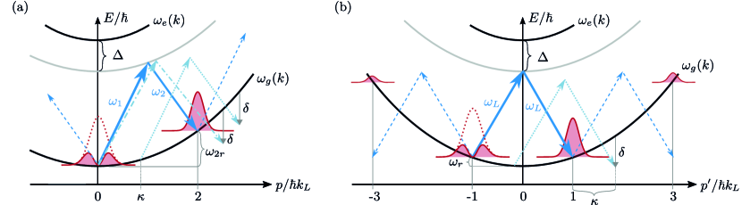
FIG. 1: Bragg diffraction: energy diagram versus atomic wavenumber $k=p/\hbar$ in units of $k_{L}$ (2) in the lab frame $S$ (a) and an inertial frame $S^{\prime}$ (b) moving with velocity $v_{g}$ (12). Ground- and excited state eigen-frequencies of a free particle are $\omega_{g}(k)$, $\omega_{e}(k)$, the two-photon and one-photon recoil frequencies $\omega_{2r}$ and $\omega_{r}$, respectively. In frame $S$, we show that a deliberate detuning $\delta\omega$ (6) of the laser frequencies $\omega_{1},\omega_{2}$ leads to the same fr6equency gap $\delta$ (7) (dashed-dotted arrows), as caused by a finite initial momentum $p_{i}=\kappa\hbar k_{L}$ (5) (dotted arrows). In frame $S^{\prime}$, the counterpropagating lasers have equal frequencies $\omega_{1,2}^{\prime}=\omega_{L}$ (2) and link $p_{i}^{\prime}=-\hbar k_{L}$ with $p_{f}^{\prime}=\hbar k_{L}$. The velocity selectivity of Bragg scattering leads to an incomplete transfer in the momentum ensembles (red, shadowed). Odd momenta $\pm 3k_{L},\pm 5k_{L},\ldots$ are populated by higher order diffraction.

In this article, we will revisit atomic beamsplitters in a moving frame in Sec. II. We compare two common methods to solve the Schrödinger equation with plane-wave laser beams in Sec. III. This is the Bloch-wave ansatz and an ad-hoc ansatz, which leads to a more convenient extended zone scheme. In Sec. IV, we study aberrations due to velocity selectivity, higher diffraction orders, spatial variations of the beam intensities, wavefront curvatures and the influence of four non-adiabatic temporal pulse envelopes in terms of the complex transfer function and the fidelity. We introduce an explicitly solvable Demkov-Kunike type model, which applies to hyperbolic sech pulses. With the full (3+1)D simulations the effects of spatially Gauss-Laguerre laser beams are studied. Finally, we gauge simulations and explicit models to experimental data in Sec. V.

II Matter-wave Bragg beamsplitter

II.1 Conservation laws

The basic mechanism of an atomic beamsplitter is the stimulated absorption and emission of two photons from bichromatic, counterpropagating laser beams [59, 1]. This process is depicted in Fig.  1a and satisfies energy and momentum conservation

$$\frac{p_{i}^{2}}{2M}+\hbar\omega_{1}=\frac{p_{f}^{2}}{2M}+\hbar\omega_{2},\qquad p_{i}+\hbar k_{1}=p_{f}-\hbar k_{2}.$$ (1)

Here, $p_{i,f}$ are the initial and final momenta of the particle with mass $M$, $\pm\hbar k_{1,2}$ are photon momenta and $\omega_{1,2}$ are the laser frequencies. We choose to work with positive wavenumbers $k_{1,2}>0$ and emphasize the propagation directions with explicit signs, but retain the directionality of $p_{i,f}$. Frequency and wavenumber are coupled by the vacuum dispersion relation $\omega=ck$, with the speed of light $c$. One chooses counterpropagating beams to maximize the momentum transfer $p_{f}-p_{i}=2\hbar k_{L}$, introducing the average wavenumber and frequency

$$k_{L}\equiv\frac{k_{1}+k_{2}}{2},\qquad\omega_{L}\equiv ck_{L}.$$ (2)

Wave mechanics considers superpositions of momentum states $\ket{g,p_{i}}$ and $\ket{g,p_{f}}$ in the internal atomic ground state $g$. For atoms initially at rest $p_{i}=0$, energy and momentum conservation (1) requires laser frequencies

$$\omega_{1}=\omega_{2}+\omega_{2r}\approx\omega_{2}+\frac{\hbar(2k_{2})^{2}}{2M}.$$ (3)

Due to the two-photon recoil, we need to introduce

$$\omega_{2r}\equiv\frac{\hbar(2k_{L})^{2}}{2M}=4\omega_{r},$$ (4)

as the two-photon frequency $\omega_{2r}$ in terms of the single photon frequency $\omega_{r}$. The approximation (3) holds for non-relativistic energies, just as the kinetic energy in (1).

II.2 Off-resonant response

Releasing ultracold atomic ensembles from traps provides localized wavepackets with a finite momentum dispersion. Therefore, one needs to study the response of the Bragg beamsplitter with finite initial- and final momenta $\bar{p}_{i}=\kappa\hbar k_{L}$, $\bar{p}_{f}=(2+\kappa)\hbar k_{L}$, introducing a dimensionless momentum $\kappa$. This opens a frequency gap

$$\mbox{$\delta$}\equiv\frac{\bar{p}_{f}^{2}}{2M\hbar}+\omega_{2}-\frac{\bar{p}_{i}^{2}}{2M\hbar}-\omega_{1}=\omega_{2r}\kappa,$$ (5)

shown in Fig. 1 (a).

Alternatively, one can also probe the momentum response by a detuning of the laser frequencies $\tilde{\omega}_{1,2}$ from the resonant values $\omega_{1,2}$ in (3). Conveniently, this detuning is measured by

$$\mbox{$\delta\omega$}\equiv\omega_{1}-\omega_{2}+\tilde{\omega}_{2}-\tilde{\omega}_{1}.$$ (6)

Dash-dotted arrows mark the deviant frequencies in Fig. 1 (a). For a particle, which is initially at rest $\tilde{p}_{i}=0$ and acquires a momentum $\tilde{p}_{f}=\hbar(\tilde{k}_{1}+\tilde{k}_{2})$ after the momentum transfer, one obtains a frequency gap

$$\mbox{$\delta$}=\frac{\tilde{p}_{f}^{2}}{2M\hbar}+\tilde{\omega}_{2}-\tilde{\omega}_{1}\approx\mbox{$\delta\omega$}.$$ (7)

The approximation holds for $|\tilde{\omega}_{1,2}-\omega_{1,2}|\ll\omega_{L}$, which is satisfied very well in the present context. Comparing Eqs. (5) and (7), one finds a linear relation

$$\mbox{$\delta\omega$}=\omega_{2r}\kappa,$$ (8)

between laser-frequency mismatch $\delta\omega$ and the dimensionless initial particle momentum $\kappa$. Therefore, both realizations are suitable to probe the momentum response of Bragg diffraction and their results are related by Eq. (8).

Experimentally, it is advantageous to modify the laser-frequencies (cf. Sec. V) and to prepare atomic wavepackets initially at rest in the lab-frame $S$. Theoretically, it is beneficial to emphasize the symmetries of the system. Therefore, we will adopt a moving inertial frame $S^{\prime}$, wherein the Doppler-shifted laser-frequencies coincide and the momentum coupled states $p_{i}^{\prime}=-\hbar k_{L}$, $p_{f}^{\prime}=+\hbar k_{L}$ are distributed symmetrically (cf. Sec. II.3, App. A). This is depicted in Fig. 1b.

II.3 Counterpropagating, bichromatic fields

The superposition of two counterpropagating laser beams $\bm{E}=\bm{E}_{1}+\bm{E}_{2}$, is defined by the constituent fields $\bm{E}_{i}=\real[\bm{E}_{i}^{(+)}]$ with the positive frequency components

$$\bm{E}_{i}^{(+)}(t,\bm{r})=\bm{\epsilon}_{i}e^{-i\phi_{i}(t,x)}\mathcal{E}_{i}(t,\bm{r}).$$ (9)

Here, $\bm{\epsilon}_{i}$ denote the polarization vectors, $\mathcal{E}_{i}(t,\bm{r})$ the slowly varying complex Gaussian envelopes and $\phi_{1}(t,x)=\omega_{1}t-k_{1}x$, $\phi_{2}(t,x)=\omega_{2}t+k_{2}x$ are the rapidly oscillating carrier phases for fields propagating along the x-direction [60] (cf. App. A and B). From the superposition of two scalar counterpropagating bichromatic fields

$$\mathcal{E}=e^{-i\phi_{1}(t,x)}\mathcal{E}_{1}+e^{-i\phi_{2}(t,x)}\mathcal{E}_{2},$$ (10)

one obtains a steady motion of the intensity pattern

$$|\mathcal{E}|^{2}=|\mathcal{E}_{1}|^{2}+|\mathcal{E}_{2}|^{2}+2\real\left[\mathcal{E}_{2}^{\ast}\mathcal{E}_{1}^{\phantom{*}}e^{i(k_{1}+k_{2})(x-v_{g}t)}\right],$$ (11)

where nodes move with the group velocity

$$v_{g}=\frac{\omega_{1}-\omega_{2}}{\omega_{1}+\omega_{2}}c,\qquad|v_{g}|=\frac{\omega_{2r}}{2\omega_{L}}c\ll c.$$ (12)

If the lab frame $S$ has the coordinates $x$, then the moving interference pattern defines another inertial frame $S^{\prime}$, where the grating is at rest and the coordinates

$$x^{\prime}=x-v_{g}t,$$ (13)

are related to the lab frame coordinates $x$ by a passive Galilean transformation.

II.4 Interaction energy

The atom is represented by a ground $\ket{g}$ and an excited state $\ket{e}$. These levels are separated by the transition frequency $\omega_{0}=\omega_{e}-\omega_{g}$ and coupled by the electric dipole matrix element $\bm{d}_{eg}=\bra{e}\hat{\bm{d}}\ket{g}$. To neglect spontaneous emissions, the lasers are far-detuned from the atomic resonance frequencies $|\omega_{0}-\omega_{i}|\gg\Gamma$, where $\Gamma$ is the natural linewidth of the transition. In the lab frame $S$ the Hamilton operator of an atom with mass $M$ reads

$$\hat{H}(t)= \frac{\hat{\bm{p}}^{2}}{2M}+\hbar\omega_{g}\hat{\sigma}_{g}+\hbar\omega_{e}\hat{\sigma}_{e}+V(t,\hat{\bm{r}}),$$ (14)

$$V(t,\bm{r})= \frac{\hbar}{2}\hat{\sigma}^{\dagger}\sum_{i=1}^{2}\Omega_{i}(t,\bm{r})e^{-i\phi_{i}(t,x)}+\text{h.c.},$$

using the spin operators $\hat{\sigma}_{i=e,g}=\outerproduct{i}{i}$ and $\hat{\sigma}=\outerproduct{g}{e}$. Here, we evaluate the electric dipole interaction energy in the rotating-wave approximation and denote the Rabi frequencies as $\Omega_{i}(t,\bm{r})=-\bm{\varepsilon}_{i}\dotproduct\bm{d}_{ge}\,\mathcal{E}_{i}(t,\bm{r})/\hbar$ .

If we transform this Hamilton operator to the frame $S^{\prime}$, comoving with the nodes of the interference pattern (13), and use a corotating internal frame (96), it reads

$$\begin{split}\hat{H}^{\prime\prime}(t)=&\frac{\hat{\bm{p}}^{2}}{2M}-\hbar\Delta\hat{\sigma}_{e}+\frac{\hbar}{2}\hat{\sigma}^{\dagger}\left[\tilde{\Omega}_{1}(t,\hat{\bm{r}})e^{ik_{L}\hat{x}}\right.\\ &+\left.\tilde{\Omega}_{2}(t,\hat{\bm{r}})e^{-ik_{L}\hat{x}}\right]+\text{h.c.}\end{split}$$ (15)

In this specific frame the atom responds only to a carrier wavenumber $k_{L}$. We measure the laser detuning $\Delta\equiv\omega_{L}-\omega_{0}$ with respect to the common Doppler-shifted frequency $\omega_{L}$. The Rabi frequencies $\tilde{\Omega}_{i}\!\left(\!t,\bm{r}\!\right)$ are given by the pulsed Gauss-Laguerre beams of Eq. (107).

Dissipative processes are not an issue for large detunings, why we can resort to the solution of the Schrödinger equation for $t>t_{i}$ and $\ket{\psi}\equiv\ket{\psi^{\prime\prime}}$

$$\ket{\psi(t)}=G(t,t_{i})\ket{\psi(t_{i})},$$ (16)

with the propagator $G(t,t_{i})$ (125).

For the numerical solution of this two-component, (3+1)D problem, we use Fourier methods with symplectic integrators [61] and operator disentangling [62]. Analytical solutions are examined for rectangular pulses (Sec. IV.3) and the hyperbolic secant pulse (Sec. IV.4).

II.5 Ideal Bragg beamsplitter and mirror

The interaction of a two-state system with laser pulses can be understood qualitatively by the “pulse area” [63]

$$\theta(t)=\int_{-\infty}^{t}\text{d}t^{\prime}\,\Omega(t^{\prime}),$$ (17)

which is rather a phase by dimension. In the context of ideal Bragg scattering, the two states are the momentum states $\{\ket{-k_{L}}_{x},\ket{k_{L}}_{x}\}$. One can visualize the evolution during the action of the Bragg pulse as a motion on the Bloch sphere [64]. A symmetrical 50:50 Bragg beamsplitter corresponds to a $\theta=\pi/2$ rotation from the south pole to the equator at some longitude. This gives equal probability to the outputs channels $\ket{\pm k_{L}}$. A $\theta=\pi$ rotation from the south pole to the north pole reverses the momenta $\ket{-k_{L}}\rightarrow\ket{k_{L}}$ and thus acts like a mirror. In the following discussion, we will focus on the mirror configuration as it is most susceptible to aberrations, due to the longer interaction time.

The polar decomposition of the transition amplitude

$$\bra{\bm{k}^{\prime}}G(t,t_{i})\ket{\bm{k}}=\sqrt{\eta_{k^{\prime}k}}e^{i\phi_{k^{\prime}k}}$$ (18)

between initial $\ket{\bm{k}}$ and final $\ket{\bm{k}^{\prime}}$ momentum states characterizes the diffraction efficiency $0\leq\eta_{k^{\prime}k}\leq 1$. For atomic wavepackets, we use the phase sensitive fidelity

$$F=|\langle\psi_{\text{ideal}}|\psi(t_{f})\rangle|^{2},\qquad\ket{\psi_{\text{ideal}}}=e^{2i\bm{k}_{L}\hat{\bm{x}}}|\psi_{i}\rangle,$$ (19)

characterizing the overlap of the final state $\ket{\psi(t_{f})}$ of Eq. (16) and the ideal final state $\ket{\psi_{\text{ideal}}}$. For an initial plane wave, the fidelity is $F=\eta_{k^{\prime}k}$ with $\bm{k}^{\prime}=\bm{k}+2\bm{k}_{L}$.

II.6 Sources of aberrations

The velocity dispersion of Bragg diffraction [55] is significant and leads to incomplete population transfer atomic wavepackets (cf. Fig. 1, Sec. IV.3.1). Another cause for population loss is off-resonant coupling to higher diffraction orders (cf. Sec. IV.3.2). This signals the crossover from the deep-Bragg towards the Raman-Nath regime, referred to as quasi-Bragg regime [51].

In general, smooth time-dependent laser pulses (cf. Sec. IV.1) lead to equally smooth beamsplitter responses (cf. Sec. IV.4 and IV.6). In contrast, smooth spatial envelopes lead to aberrations (cf. Sec. IV.7). Every Gauss-Laguerre beam exhibits spatial inhomogeneity and wavefront curvature. This is relevant for atomic clouds that are comparable in size to the laser beam waist, or for clouds displaced from the symmetry axis. Static laser misalignment further degrades the diffraction efficiency.

There are sundry other dynamical sources of aberrations, such as mechanical vibrations of optical elements or stochastic laser noise [65]. The fundamental process of spontaneous emission leads to decoherence and aberrations, too. Fortunately, this can be suppressed by a detuning $|\Delta|\gg\Gamma$ much larger than the linewidth $\Gamma$, as well as limiting the interaction time.

III Plane-wave approximation

The basic mechanism of Bragg beamsplitters arises from the momentum transfer of plane waves with a real, constant Rabi frequency $\tilde{\Omega}_{1}(t,\bm{r})=\tilde{\Omega}_{2}(t,\bm{r})=\Omega_{0}$ within the duration of a rectangular pulse. This model is the reference to gauge more realistic calculations. Consequently, the two components $\{\psi_{e}(t,\bm{r}),\psi_{g}(t,\bm{r})\}$ of the Schrödinger field evolve according to

$$i\partial_{t}\psi_{e}=\left(-\frac{\hbar}{2M}\nabla^{2}-\Delta\right)\psi_{e}+\Omega_{0}\cos(k_{L}x)\psi_{g},$$ (20a)

$$i\partial_{t}\psi_{g}=-\frac{\hbar}{2M}\nabla^{2}\psi_{g}+\Omega_{0}^{\ast}\cos(k_{L}x)\psi_{e}.$$ (20b)

using the Hamilton operator (15). Assuming the excited state is initially empty, the atom’s kinetic energy is small and the lasers are far-detuned $|\Delta|\gg\Gamma,\ \Omega_{0},\ \omega_{r}$, we can adiabatically eliminate the excited state [66, 51]

$$\psi_{e}\approx\frac{\Omega_{0}}{\Delta}\cos(k_{L}x)\psi_{g}.$$ (21)

Then, the ground state Schrödinger equation reads

$$i\partial_{t}\psi_{g}=\left(-\frac{\hbar}{2M}\bm{\nabla}^{2}+\mathcal{V}(x)\right)\psi_{g},$$ (22)

with the dipole potential $\mathcal{V}(x)=\cos^{2}\!\left(\!k_{L}x\!\right)|\Omega_{0}|^{2}/\Delta$ [67]. Stationary solutions of the one-dimensional problem are Mathieu functions [68]. Our goal is to formulate a suitable ansatz for the (3+1) dimensional non-separable equation with time-dependent pulses.

III.1 Bloch-wave ansatz

The Bloch picture is suitable for describing the velocity selective atomic diffraction by a standing laser wave [1, 69, 70]. The characteristic translation invariance of the Hamilton operator (22) by a displacement of $a_{x}=\lambda_{L}/2$ defines a natural length scale. Its reciprocal is the lattice vector $\mathfrak{q}_{x}=2\pi/a_{x}=2k_{L}$. It is convenient to embed the total three-dimensional wavefunction in an orthorohmbic volume with lengths $(N_{x}a_{x},a_{y},a_{z})$, with $N_{x}\in\mathbb{N}$ and to impose periodic boundary conditions $\psi_{g}(x+N_{x}a_{x},y+a_{y},z+a_{z})=\psi_{g}(x,y,z)$. Bragg scattering involves at least two photons, one from each of the counterpropagating lasers. Therefore, the two-photon recoil frequency $\omega_{2r}$ (4) emerges as the frequency scale. In terms of the dimensionless length $\xi=\mathfrak{q}_{x}x$ and time $\tau=\omega_{2r}t$, the Schrödinger field

$$\psi_{g}(t,\bm{r})=\sum_{r=-\left\lfloor\frac{N_{y}}{2}\right\rfloor}^{\left\lceil\frac{N_{y}}{2}\right\rceil-1}\sum_{s=-\left\lfloor\frac{N_{z}}{2}\right\rfloor}^{\left\lceil\frac{N_{z}}{2}\right\rceil-1}e^{i(r\mathfrak{q}_{y}y+s\mathfrak{q}_{z}z-\bar{\omega}_{r,s}\tau)}h^{(r,s)}(\tau,\xi),$$ (23)

factorizes into one-dimensional fields $h^{(r,s)}(\tau,\xi)$ and two-dimensional plane waves with the transversal lattice vectors $\mathfrak{q}_{y,z}=2\pi/a_{y,z}$. The integers $N_{y,z}\in\mathbb{N}$ define the maximal momentum resolution $\mathfrak{q}_{i}^{\text{max}}=\mathfrak{q}_{i}\left\lfloor N_{i}/2\right\rfloor$. Please note the use of the Gauss brackets rounding towards the nearest integer at the “floor” $\left\lfloor\,\right\rfloor$ or the “ceiling” $\left\lceil\,\right\rceil$. With a detuning dependent shift of the frequency, introducing the two-photon Rabi frequency $\Omega$,

$$\bar{\omega}_{r,s} =\hbar\frac{r^{2}\mathfrak{q}_{y}^{2}+s^{2}\mathfrak{q}_{z}^{2}}{2M\omega_{2r}}+\Omega, \Omega =\frac{\Omega_{r}}{\omega_{2r}}=\frac{|\Omega_{0}|^{2}}{2\omega_{2r}\Delta},$$ (24)

the Schrödinger equation for each amplitude simplifies to

$$i\partial_{\tau}h(\tau,\xi)=\left(-\partial^{2}_{\xi}+\Omega\cos{\xi}\right)h(\tau,\xi).$$ (25)

By construction, the potential is $2\pi$-periodic and the eigenfunctions $h(\tau,\xi)=e^{-i\tau\omega^{(b)}(q)}h^{(b)}(\xi,q)$ are given by Bloch-waves $h^{(b)}(\xi,q)$ [71, 72, 73, 74] with the lattice periodic function $g^{(b)}(\xi,q)$ for momentum $q$ and band index $b$

$$h^{(b)}(\xi,q) =e^{iq\xi}g^{(b)}(\xi,q),$$ (26)

$$g^{(b)}(\xi+2\pi,q) =g^{(b)}(\xi,q).$$ (27)

From the periodic boundary conditions for the wavefunction $h^{(b)}(\xi+2\pi N_{x},q)=h^{(b)}(\xi,q)$, one obtains a quantization of the wavenumber $q_{n}=n/N_{x}$ with $n\in\mathbb{Z}$. The interval $-1/2\leq q_{n}<1/2$ defines the first Brillouin zone in the reduced zone scheme, whose extent equals the crystal momentum $Q=1$.

Bloch wavefunctions are also periodic in momentum space $h^{(b)}(\xi,q+Q)=h^{(b)}(\xi,q)$, provided we define

$$g^{(b)}(\xi,q)=\sum_{m=-\mathcal{N}}^{\mathcal{N}-1}e^{im\xi}g^{(b)}(m+q),$$ (28)

by a Fourier series for a maximal diffraction order $\mathcal{N}\in\mathbb{N}$ with boundary condition$g^{(b)}\left(q+\mathcal{N}\right)=g^{(b)}\left(q-\mathcal{N}\right)=0$. From a superposition of these Bloch waves, one obtains the ansatz

$$h(\tau,\xi)=\sum_{n=-\left\lfloor\frac{N_{x}}{2}\right\rfloor}^{\left\lceil\frac{N_{x}}{2}\right\rceil-1}\sum_{m=-\mathcal{N}}^{\mathcal{N}-1}e^{i(m+q_{n})\xi}g(\tau,m+q_{n}),$$ (29)

for the time-dependent solution of Eq. (25), compatible with the Bloch theorem and suitable for numerical computation. This ansatz transforms the partial differential equation into the parametric difference equation

$$i\partial_{\tau}g_{m}(\tau,q)=(m+q)^{2}g_{m}+\tfrac{\Omega}{2}(g_{m+1}+g_{m-1}).$$ (30)

The $q$-dependence of the $m^{th}$-order scattering amplitude $g_{m}(\tau,q)\equiv g(\tau,m+q)$ leads to the velocity dispersion of Bragg diffraction. Assuming Dirichlet boundary conditions, one can use a $(2\mathcal{N}-1)$-dimensional representation $\bm{g}^{e}=(g_{-(\mathcal{N}-1)},\ldots,g_{\mathcal{N}-1}),$ to study the initial value problem

$$i\dot{\bm{g}}^{e}=H^{e}(q)\bm{g}^{e},\qquad H^{e}=D^{e}+L+L^{\dagger}.$$ (31)

For the indices $1-\mathcal{N}\leq m\leq\mathcal{N}-1$, the Hamilton matrix $H^{e}$ is formed by a diagonal matrix $D^{e}$ and a lower triangular matrix $L$

$$D^{e}_{m,n}=(m+q)^{2}\delta_{m,n},\qquad L_{m,n}=\tfrac{\Omega}{2}\delta_{m,n+1}.$$ (32)

In order to study the discrete Bloch energy bands $\omega^{(b)}(q)$, one has to solve the eigenvalue problem

$$\bm{g}^{e}(\tau,q)=e^{-i\tau\omega(q)}\bm{g}^{e}(q),\qquad\omega(q)\bm{g}^{e}=H^{e}(q)\bm{g}^{e}.$$ (33)

In Fig. 2, we present the lowest few energy bands $\omega^{(b)}(q)$ versus the lattice momentum $q$ in an extended momentum zone scheme. For reference, we depict the quadratic dispersion relation of the empty lattice $\Omega\!=\!0$ and the dispersion relation for $\Omega\!=\!1$ ($\Omega_{r}\!=\!\Omega\,\omega_{2r}\!=\!4\,\omega_{r}$), a moderately deep lattice. Narrow momentum wavepackets $\psi(k)$ with $\sigma_{k}\ll k_{L}$ are ideal for beamsplitters. If they are located at the band edges $k\!=\!q\mathfrak{q}_{x}\!=\!(\pm 1/2+m)2k_{L}$, the two-photon process covers at least three Brillouin zones. For wavepackets at the center $k\!=\!q\mathfrak{q}_{x}\!=\!2mk_{L}$, only two Brillouin zones are coupled by a Bragg pulse.

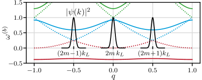
FIG. 2: Energy bands $\omega^{(0,1,2)}(q)$ of a periodic lattice in the extended zone scheme versus quasi-momentum $q$, with empty lattice $\Omega=0$ (dotted) and finite depth $\Omega=1$ (solid), where $\Omega_{r}\!=\!\Omega\,\omega_{2r}\!=\!4\,\omega_{r}$. Initial wavepackets with odd momenta $(2m+1)k_{L}$ are located at the edges $q\!=\!\pm 1/2$ of the $1^{st}$ Brillouin zone, while even momenta $2mk_{L}$ are at the center $q=0$.

III.2 Ad-hoc ansatz

There are alternatives formulations [51, 55] to the Bloch-wave ansatz, if we define a Fourier series on the periodic lattice $h(x+N_{x}a_{x})=h(x)$ as

$$h(x)=\sum_{l=-\infty}^{\infty}e^{i\frac{2\pi l}{N_{x}a_{x}}x}g_{l},\qquad\frac{2\pi l}{N_{x}a_{x}}=\frac{2l}{N_{x}}k_{L}.$$ (34)

By decomposing the index $l=N_{x}m+r$ into a quotient $m=\left\lfloor l/N_{x}\right\rfloor$ and a remainder $0\leq r<N_{x}$, one obtains

$$h(x)=\sum_{n=-\left\lfloor\frac{N_{x}}{2}\right\rfloor}^{\left\lceil\frac{N_{x}}{2}\right\rceil-1}\sum_{m=-\mathcal{N}}^{\mathcal{N}-1}g_{2m+1}(\kappa_{n})e^{ik_{2m+1}^{n}x},$$ (35)

with $n=r-\left\lfloor N_{x}/2\right\rfloor$. In this series, we use a momentum $k_{\mu}^{n}=(\mu+\kappa_{n})k_{L}$ and a quasimomentum $\kappa_{n}$

$$-1\leq\kappa_{n}=\frac{2n}{N_{x}}-\frac{\left\lceil\frac{N_{x}}{2}\right\rceil-\left\lfloor\frac{N_{x}}{2}\right\rfloor}{N_{x}}<1,$$ (36)

in an extended Brillouin zone. As the Schrödinger equation (25) has even parity, parity is a conserved quantity. An ansatz with $\sin$ and $\cos$ functions would lead to a decoupling of (35) with respect to parity manifolds.

The decomposition of the index $l=N_{x}m+n$ is not unique, if we admit signed integral remainders within the limits $-\left\lfloor N_{x}/2\right\rfloor\leq n<\left\lceil N_{x}/2\right\rceil$. This implies a quotient $m=\left\lfloor(l+\left\lfloor N_{x}/2\right\rfloor)/N_{x}\right\rfloor$. Now, the Fourier series reads

$$h(x)=\sum_{n=-\left\lfloor\frac{N_{x}}{2}\right\rfloor}^{\left\lceil\frac{N_{x}}{2}\right\rceil-1}\sum_{m=-\mathcal{N}}^{\mathcal{N}-1}g_{2m}(\kappa_{n})e^{ik_{2m}^{n}x},$$ (37)

with the quasimomentum $\kappa_{n}$

$$-1\leq\kappa_{n}=\frac{2n}{N_{x}}\leq 1-\frac{1}{N_{x}}.$$ (38)

The definitions of the quasimomenta in Eqs. (36) and (38), agree exactly for even number $N_{x}=2u$ of lattice sites or coincide asymptotically for $N_{x}\rightarrow\infty$. The even/odd ambiguity of number of lattice sites can not be of physical significance as the periodic boundary condition are mere mathematical convenience. Therefore, assuming an even number of lattice sites is no limitation.

Using time-dependent amplitudes $g_{\mu}(\tau,\kappa_{n})$ in the series (35) and (37), transforms the Schrödinger equation (25) into a single difference equation $\forall\mu\in\mathbb{Z}$

$$i\partial_{\tau}g_{\mu}(\tau,\kappa)=\tfrac{1}{4}(\mu+\kappa)^{2}g_{\mu}+\tfrac{\Omega}{2}(g_{\mu+2}+g_{\mu-2}).$$ (39)

Due to the two-photon transfer, there is no coupling between even and odd solution manifolds. Consequently, it is advantageous to use Eq. (35) for wavepackets located around odd multiples of $k_{L}$ or Eq. (37) for even multiples of $k_{L}$ (cf. Fig. 2). As in the comoving frame $S^{\prime}$ (13) mainly $\ket{-k_{L}}$ is coupled with $\ket{+k_{L}}$, we focus on the odd solution manifold with $\mu=2m+1$. Therefore, Eq. (39) can be cast into a tridiagonal system of linear differential equations

$$i\dot{\bm{g}}^{o}=H^{o}\bm{g}^{o},\qquad H^{o}=D^{o}+L+L^{\dagger},$$ (40)

for $\bm{g}^{o}=(g_{-2\mathcal{N}+1},g_{-2\mathcal{N}+3},\ldots g_{2\mathcal{N}-1})$ with $L$ from (32) and a diagonal matrix

$$D^{o}_{\mu,\nu}=\tfrac{1}{4}(\mu+\kappa)^{2}\delta_{\mu,\nu}\equiv D_{\mu,\nu}+\varpi\delta_{\mu,\nu}.$$ (41)

In the following, it will be prudent to adopt a rotating frame $\bm{g}^{o}(\tau)=e^{-i\varpi\tau}\bm{g}(\tau)$ with a frequency offset denoted by $\varpi=(-1+\kappa)^{2}/4$

$$i\dot{\bm{g}}=\mathcal{H}\bm{g},\qquad\mathcal{H}=D+L+L^{\dagger},$$ (42)

$$D_{\mu,\nu}=\omega_{\mu}\delta_{\mu,\nu},\qquad\omega_{\mu}=\tfrac{1}{4}(\mu+\kappa)^{2}-\varpi.$$ (43)

This grounds the frequency $\omega_{-1}=0$.

IV Aberration analysis

Using the ad-hoc ansatz for Bragg scattering, we will successively consider more realistic processes to assess their contribution to aberrations. We begin with the plane-wave approximation and consider four temporal Bragg-pulse shapes $f_{i}(\tau)$. We will analyze their influence on the velocity dispersion as well as losses into higher diffraction orders. Finally, we will add the spatial envelopes of the Gaussian-Laguerre beams and consider the cumulative effect.

IV.1 Bragg-pulse shapes

We examine temporal Gaussian- (G), rectangular- (R), hyperbolic secant- (S) and Blackman- (B) Rabi pulses

$$\Omega(\tau)=\Omega f_{j}(\tau),\quad j\in\{G,R,S,B\}.$$ (44)

The shape functions $f_{j}$, depicted in Fig.  3, are all normalized to unity at maximum and characterized by a window width $\tau_{j}$. Different Rabi pulses (44) can be compared physically, if they cover the same pulse area (17)

$$\theta \equiv\theta(\tau=\infty)=\Omega T,$$ (45a)

$$T \equiv T(-\infty,\infty),\quad T(\tau_{i},\tau_{f})=\int_{\tau_{i}}^{\tau_{f}}\text{d}\tau\,f_{j}(\tau),\vspace{-7mm}$$ (45b)

for equal nominal time $T=T_{G}=T_{R}=T_{B}=T_{S}$.
Rectangular pulses are popular in theory as they are constant during the interaction time and lead to simple analytical approximations. They read

$$f_{R}(|\tau|\leq\tau_{R})=1,\qquad T_{R}=2\tau_{R}$$ (46)

and $f_{R}(|\tau|>\tau_{R})=0$, elsewhere.
Gaussian pulses are the standard shapes in pulsed laser experiments

$$f_{G}(\tau)=e^{-\frac{\tau^{2}}{2\tau^{2}_{G}}},\qquad T_{G}=\sqrt{2\pi}\,\tau_{G},$$ (47)

with Gaussian width $\tau_{G}$.
Blackman pulses are characterized by a window function

$$f_{B}(\tau) =w_{B}\negthinspace\left(\frac{\tau}{\tau_{B}}\right),\qquad T_{B}=\frac{21\pi}{25}\tau_{B},$$ (48)

$$w_{B}(|\phi|\leq\pi) =\tfrac{1}{50}[21+25\cos(\phi)+4\cos(2\phi)]$$ (49)

and $w_{B}(|\phi|>\pi)=0$ elsewhere.
Hyperbolic secant pulses are defined with

$$f_{S}(\tau)=\sech\left(\frac{\tau}{\tau_{S}}\right),\qquad T_{S}=\pi\tau_{S}.$$ (50)

They are amenable for analytical solutions [75, 76].

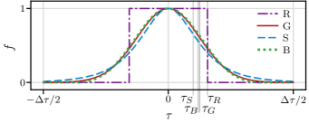
FIG. 3: Temporal envelopes $f(\tau)$ for rectangular-, Gaussian-, hyperbolic secant- and Blackman pulses for equal nominal time $T=T_{j}$, $j\in\{G,R,S,B\}$ and total pulse length $\Delta\tau=8\,\tau_{G}$. The vertical lines indicates the pulse widths $\tau_{j}$.

IV.2 Definition of $\pi$- and $\frac{\pi}{2}$-pulses

The symmetrical 50:50 beamsplitter pulse and the 0:100 mirror pulse are the two most relevant applications of atomic Bragg diffraction (cf. Sec. II.5). Irrespective of the shape, a symmetrical beamsplitter pulse is defined by a pulse area of $\theta=\pi/2$, while a complete specular reflection in momentum space is achieved for $\theta=\pi$. This defines the nominal times

$$T_{\pi}=\frac{\pi}{|\Omega|},\qquad T_{\pi/2}=\frac{T_{\pi}}{2}.$$ (51)

In particular, the four pulse shapes yield mirror widths

$$\tau_{G\pi}\!=\!\frac{\sqrt{\pi}}{\sqrt{2}|\Omega|},\ \tau_{R\pi}\!=\!\frac{\pi}{2|\Omega|},\ \tau_{B\pi}\!=\!\frac{25}{21|\Omega|},\ \tau_{S\pi}\!=\!\frac{1}{|\Omega|}.$$ (52)

Due to the linearity, the symmetric beamsplitter width is just a half of the mirror time i. e., $\tau_{\pi/2}=\tau_{\pi}/2$.

IV.3 Diffraction efficiency of a rectangular pulse

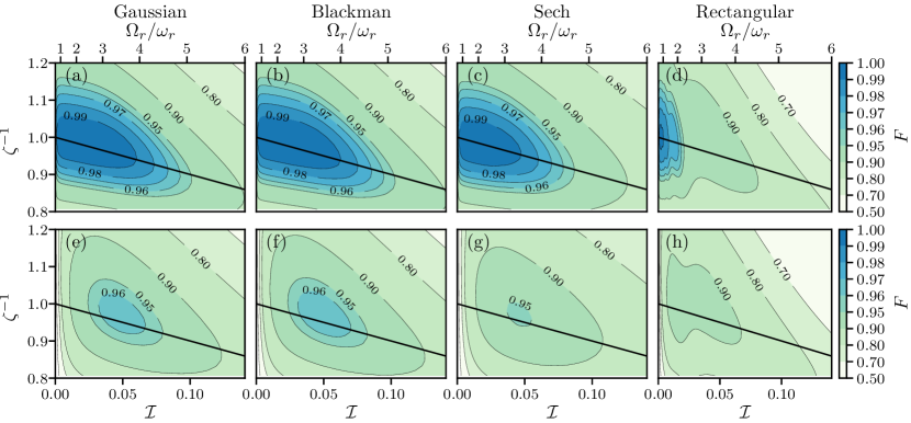
FIG. 4: Fidelity $F$ versus two-photon intensity $\mathcal{I}=\Omega^{2}/16$, respectively two-photon Rabi frequency $\Omega_{r}=\Omega\omega_{2r}$, and inverse $\pi$-pulse stretching factor $\zeta^{-1}=\tau_{j\pi}/\tau_{j}$, $j\in\{G,B,S,R\}$, for Gaussian (a, e), Blackman (b, f), sech (c, g) and rectangular pulses (d, h). The initial state is a 1D Gaussian wavepacket (98), initially centered at $(x,k_{x})=(0,-k_{L})$ with momentum width $\sigma_{k}=0.01\,k_{L}$ (top), $\sigma_{k}=0.1\,k_{L}$ (bottom). The optimal stretching factor $\zeta_{\pi}$ (60) (solid line) traverses the regions of maximal fidelity. For the numerical (1+1)D integration (16) with pulse widths $\zeta\tau_{j\pi}$, and total pulse length $\Delta\tau_{j}=8\zeta\tau_{G}$, typical laser and atom parameters, used in experiments (Tab. 2), are applied.

IV.3.1 Velocity selective Pendellösung

In the deep-Bragg regime $\mathcal{N}=1$, off-resonant diffraction orders are negligible. Thus, for first order diffraction $N=1$ the state vector in the beamsplitter manifold

$$k_{\pm}\equiv(\pm 1+\kappa)k_{L},$$ (53)

simplifies to the amplitude tuple $\mathbf{g}_{\mp}(\tau)=(g_{-1},g_{+1})$ with $\mathbf{g}_{\mp}(\tau_{i})=(1,0)$. The well known Pendellösung [77, 78]

$$\begin{split}g_{-1}(\tau)&=e^{-i\varphi}\left(\cos\vartheta-\frac{\kappa}{i\Omega_{\kappa}}\sin\vartheta\right),\\ g_{+1}(\tau)&=e^{-i\varphi}\frac{\Omega}{i\Omega_{\kappa}}\sin\vartheta,\end{split}$$ (54)

depends on $\varphi=\kappa(\tau-\tau_{i})/2$, $\vartheta=\Omega_{\kappa}(\tau-\tau_{i})/2$ and the generalized two-photon Rabi frequency $\Omega_{\kappa}=\sqrt{\kappa^{2}+\Omega^{2}}$. It follows from (42) for the rectangular pulse shape (46)

$$i\dot{\bm{g}}_{\mp}(\tau)=\mathcal{H}_{\mp}\bm{g}_{\mp},\qquad\mathcal{H}_{\mp}=\begin{pmatrix}0&\frac{\Omega}{2}\\ \frac{\Omega}{2}&\kappa\end{pmatrix}.$$ (55)

With this solution the mirror pulse width (52) can be generalized for arbitrary $\kappa\neq 0$. Maximal efficiency $\eta_{+-}(\tau_{R\pi})=|g_{+1}(\tau_{\pi})|^{2}$ is achieved for $\vartheta=\pi/2$, which determines the mirror pulse width

$$\tau_{R\pi}(\kappa)=\frac{\pi}{2\Omega_{\kappa}}.$$ (56)

On resonance ($\kappa=0$), we recover Eq. (52). Finally, the diffraction efficiency reads

$$\eta_{+-}(\tau_{R\pi})=\frac{\Omega^{2}}{\Omega_{\kappa}^{2}}\sin^{2}{\vartheta_{\pi}},\qquad\vartheta_{\pi}=\frac{\pi}{2}\frac{\Omega_{\kappa}}{\Omega}.$$ (57)

The relative phase of the transfer function (18), between the final $k_{-}$ and $k_{+}$ components is

$$\Delta\phi\equiv\phi_{--}-\phi_{+-}=\arctan\!\left(\!\frac{\kappa}{\Omega_{\kappa}}\tan\vartheta\!\right)\!-\negmedspace\frac{\pi}{2}.$$ (58)

For $\vartheta=\vartheta_{\pi}$, one obtains the phase shift after a mirror pulse $\Delta\phi(\tau_{R\pi})$.

IV.3.2 Losses into higher diffraction orders

The transfer function $\bra{\bm{k}^{\prime}}G(t,t_{i})\ket{\bm{k}}$ (18) exhibits resonances at $\bm{k}^{\prime}=\bm{k}+2N\bm{k}_{L}$. On the one hand, resonances with $N\neq 1$ lead to a population loss from the $N=1$ beamsplitter manifold $\{k_{\pm}\}$ and reduce the diffraction efficiency. On the other hand, they diminish the coupling strength within the beamsplitter manifold. Consequently, this increases the optimal $\pi$-pulse time $\tilde{\tau}_{\pi}>\tau_{\pi}$ of a Bragg mirror compared to the prediction of the Pendellösung (52). Gochnauer et al. [56] have demonstrated this effect experimentally for Gaussian pulses, proving that the effective coupling strength is given by the energy bandgap in the quasimomentum space.

Renormalized $\pi$-pulse time

The influence of higher order resonances on the beamsplitter manifold can be calculated perturbatively in terms of the generalized two-photon Rabi frequency $\Omega_{\kappa}$. For $\Omega_{\kappa}\rightarrow 0$ all momentum states are doubly degenerate with respect to their energies. We employ Kato’s perturbation theory [79], as it can describe the generalized degenerate eigenvalue problem (109). Remarkably, Kato’s 1^st order perturbation theory coincides with the Pendellösung (cf. App. C)

From a third order perturbation calculation $\mathcal{O}(\Omega_{\kappa}^{4})$, we find the renormalized Rabi frequency

$$\tilde{\Omega}=\sqrt{\kappa^{2}(1+2\mathcal{I})^{2}+\Omega^{2}(1-\mathcal{I})^{2}}\stackrel{{\scriptstyle\mathcal{I}\ll 1}}{{\longrightarrow}}\Omega_{\kappa}$$ (59)

within the beamsplitter manifold using the abbreviation $\mathcal{I}=\Omega^{2}/16$. For weak dressing $\mathcal{I}\ll 1$, it reduces to the generalized Rabi frequency of the Pendellösung. From (52), one can evaluate the $\pi$-pulse time stretching factor

$$\zeta_{\pi}^{\kappa}\!=\!\frac{\tilde{\tau}_{R\pi}}{\tau_{R\pi}}\!=\!\frac{\Omega_{\kappa}}{\tilde{\Omega}},\qquad\zeta_{\pi}\equiv\zeta_{\pi}^{\kappa=0}\!=\frac{1}{1-\mathcal{I}}\approx\!1+\mathcal{I}.$$ (60)

Figure 4 depicts a contour plot of the fidelity $F(\mathcal{I},\zeta)$ (19) for a Bragg-mirror pulse versus the bare two-photon intensity $\mathcal{I}$ and the inverse pulse stretching factor $\zeta^{-1}=\tau_{j\pi}/\tau_{j}$. This representation uncovers a linear relation. The numerically calculated fidelity (19) considers four off-resonant diffraction orders ($\mathcal{N}=5$). As initial condition, we consider 1D Gaussian wavepackets (98) centered at $k_{0}=-k_{L}$ with momentum width $\sigma_{k}$, localized in the center of the laser beams $x_{0}=0$. Here, in the plane-wave approximation, the results are independent of the expansion size. This size $\sigma_{x}=(2\sigma_{k})^{-1}$ follows from the Heisenberg uncertainty.

Clearly, the $\pi$-pulse stretching factor $\zeta_{\pi}$ (60) traverses the optimal fidelity regions for all pulse shapes and momentum widths, as a universal rule, motivating the effective $\pi$-pulse widths

$$\tilde{\tau}_{j\pi}=\zeta_{\pi}\tau_{j\pi},\quad j\in\{G,R,B,S\},$$ (61)

with $\tau_{j\pi}$ from Eq. (52).

Renormalized $\pi$-pulse efficiency

In Fig. 5 the velocity dispersion of the response of an atomic mirror is visualized for typical parameters used in experiments (cf. Tab. 2) and a two-photon Rabi frequency $\Omega_{r}=\Omega\omega_{2r}=3\omega_{r}$.

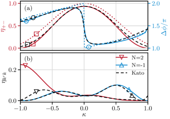
FIG. 5: (a) Diffraction efficiency $\eta_{+-}$ ($\bm{\square}$) in the beamsplitter manifold $N\!=\!1$, together with the relative phase shift $\Delta\phi$ (58) ($\bm{\circ}$) and (b) losses into higher diffraction orders $N\!\neq\!1$ versus detuning $\kappa$, after a rectangular mirror pulse. For the numerical solution (solid), considering four off-resonant diffraction orders (with $k=(-1+\kappa)k_{L}$ and $k^{\prime}\!=\!k+2Nk_{L}$) the applied pulse width is $\tilde{\tau}_{R\pi}(\Omega)$ (61) and for the Pendellösung (57), (58) (dotted), considering only the resonant diffraction order, $\tau_{R\pi}(\Omega)$ (52) for $\Omega_{r}\!=\!\Omega\,\omega_{2r}\!=\!3\,\mathrm{\omega_{r}}$. In (a), the Pendellösung overestimates the efficiency and phase shift, while the Kato corrections (121) (dashed) match the numerical results (solid) much better. There are only deviations at the band edges, especially for $N\!=\!2$ (b).

The Pendellösung (54), valid in the deep-Bragg regime ($\mathcal{N}=1$), applying the pulse width $\tau_{R\pi}(\Omega)$ (52), is compared to the eigenvalue solution (42) with pulse width $\tilde{\tau}_{R\pi}(\Omega)$ (61). Therefore, the diffraction efficiency $\eta_{k^{\prime}k}$ reveals the velocity selectivity of the Bragg condition and the population loss into higher diffraction orders, here in the quasi-Bragg regime ($\mathcal{N}=5$). The phase difference $\Delta\phi$ (58) shows a $\pi$ jump at resonance. The perturbative Kato solution (121) describes the beamsplitter response very well, only at the band edges $\kappa\rightarrow\pm 1$, there are small deviations. For weak coupling $\Omega$, the diffraction efficiency after a mirror pulse of width $\tilde{\tau}_{\pi R}(\Omega)$ (61), exhibits a sinc behavior [cf. Fig. 6 (a)]. It is the typical Fourier-response to a rectangular pulse. Increasing the Rabi frequency $\Omega$, the response is power broadened, in conjunction with a reduced efficiency. Simultaneously, the Kato solution becomes less accurate for $|\kappa|>0$, while the resonant efficiency $\eta_{0}\equiv\eta_{+-}(\kappa=0)=\eta_{k_{L},-k_{L}}$ can be approximated further. This is also depicted in Fig. 6 (b), together with the efficiency’s full width half maximum $\Delta\eta$ of the Bragg mirror. For an ideal mirror, $\eta_{0}=1$ and $\Delta\eta\rightarrow\infty$ are desirable, but impossible.

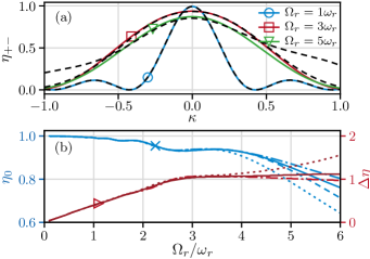
FIG. 6: (a) Diffraction efficiency $\eta_{+-}$ after a mirror pulse of width $\tilde{\tau}_{R\pi}(\Omega)$ (61) versus detuning $\kappa$ for different two-photon Rabi frequencies $\Omega_{r}=\Omega\,\omega_{2r}$, numerical results (solid) and Kato (121) solution (dashed). (b) Resonant transfer efficiency $\eta_{0}$ ($\bm{\times}$) and efficiency width $\Delta\eta$ ($\bm{\triangleright}$) versus $\Omega_{r}$. The numerically optimal interaction time, for maximal efficiency (dash-dotted) is compared to the approximations for the $\pi$-pulse width $\tau_{R\pi}$ (52) (dotted) and $\tilde{\tau}_{R\pi}$ (61) (solid). The analytical Kato approximation $\eta_{0}^{K}(\tilde{\tau}_{R\pi})$ (62) (dashed) provides meaningful predictions.

In addition, we study the optimal interaction time in Fig. 6 (b). The approximation $\tau_{R\pi}$ (52) for the deep-Bragg regime and $\tilde{\tau}_{R\pi}$ (61) for the quasi-Bragg regime, considering higher diffraction orders, are compared to the optimal interaction time, defined by the maximum numerical transfer efficiency at resonance $\kappa=0$. With increasing $\Omega$, in a regime where the losses into higher diffraction orders are important, the approximation with $\tau_{R\pi}$ is less accurate, while $\tilde{\tau}_{R\pi}$ can be used further. Please note that for the maximized transfer efficiency the velocity acceptance $\Delta\eta$ is reduced, while for $\tilde{\tau}_{R\pi}$ it remains larger, for increasing $\Omega$. From the Kato solution (121) a simple analytic equation for the diffraction efficiency on resonance, for the effective $\pi$-pulse time $\tilde{\tau}_{R\pi}$ can be derived (cf. App. C) to

$$\eta_{0}^{K}(\tilde{\tau}_{R\pi})=(1-2\mathcal{I})\left[1+|\Omega|\mathcal{I}\sin\left(\frac{2\pi}{|\Omega|}\frac{1+2\mathcal{I}}{1-\mathcal{I}}\right)\right],$$ (62)

also depicted in Fig. 6 (b). This expression predicts losses into higher diffraction orders within the convergence radius $\Omega_{r}=\Omega\,\omega_{2r}<4\,\omega_{r}$ ($\mathcal{I}<0.0625$), very well. The approximation remains positive for $\Omega_{r}<8\sqrt{2}\,\omega_{r}$ $(\mathcal{I}=0.5)$.

IV.4 Diffraction efficiency of a sech pulse

IV.4.1 Velocity selective Demkov-Kunike Pendellösung

For hyperbolic secant pulses $\Omega(\tau)=\Omega f_{S}(\tau)$ (50), one can solve Eq. (55) also in a closed form [75, 76]. A decoupling of the first order differential equation system with $g_{+1}=2i\Omega(\tau)^{-1}\dot{g}_{-1}$, leads to Hill’s second order differential equation [68]

$$0=\ddot{g}_{-1}-\biggl{(}\frac{\dot{\Omega}(\tau)}{\Omega(\tau)}-i\kappa\biggr{)}\,\dot{g}_{-1}+\frac{\Omega(\tau)^{2}}{4}g_{-1}.$$ (63)

With the nonlinear map $z(\tau)=[1+\tanh{(\tau/\tau_{S})}]/2$, the differential equation for $\gamma(z)\equiv g_{-1}(\tau)$ emerges as

$$z(1-z)\gamma^{\prime\prime}+\left[c-z(1+a+b)\right]\gamma^{\prime}-ab\gamma=0,$$ (64)

with $a=\Omega\tau_{S}/2$, $b=-a$ and $c=(1+i\kappa\tau_{S})/2$. This is the hypergeometric differential equation with solutions $f_{1}={}_{2}F_{1}(a,b;c;z),f_{2}=z^{1-c}{}_{2}F_{1}(1+a-c,1+b-c;2-c;z)$ and Wronski determinant $w=(1-z)^{c-1}z^{-c}$. Straightforward analysis (cf. App. D) leads to the Demkov-Kunike (DK) solution with unitary propagator $G_{\mp}(\tau,\tau_{i})$

$$\bm{g}_{\mp}(\tau)=G_{\mp}(\tau,\tau_{i})\bm{g}_{\mp}(\tau_{i}),\qquad G_{\mp}(\tau_{i},\tau_{i})=\mathds{1}.$$ (65)

For the initial datum $\bm{g}_{\mp}(\tau_{i})=(1,0)$, one obtains

$$g_{-1}(\tau)=[f_{1}(\tau)f^{\prime}_{2}(\tau_{i})-f_{2}(\tau)f^{\prime}_{1}(\tau_{i})]/w(\tau_{i}).$$ (66)

For a pulse beginning in the remote past $\tau_{i}\ll-\tau_{S}$, this simplifies to

$$g_{-1}(\tau) =\ _{2}F_{1}\left(a,-a;c,z\right),$$ (67)

$$g_{+1}(\tau) =\tfrac{a}{ic}\sqrt{z(1-z)}\ _{2}F_{1}\left(1-a,1+a;1+c,z\right).$$ (68)

Now, the diffraction efficiency of a beamsplitter reads

$$\eta_{+-}^{{DK}}(\kappa,\tau)=|g_{+1}(\tau)|^{2}=1-|g_{-1}(\tau)|^{2}.$$ (69)

Furthermore, for very long pulse durations $\tau_{S}\ll\tau_{f},|\tau_{i}|$, the diffraction efficiency simplifies to

$$\eta_{+-}^{{DK}}(\kappa,\Omega,T)=\sech^{2}\!\left(\frac{\kappa T}{2}\right)\sin^{2}\!\left(\frac{\Omega T}{2}\right)\!,$$ (70)

with the nominal time $T$ (45). In order to achieve full diffraction efficiency $\eta_{0}^{{DK}}=\eta_{+-}^{{DK}}(\kappa=0)=1$, one should choose the $\pi$-pulse width as $\tau_{S\pi}=|\Omega|^{-1}$, in agreement with the pulse area (52). Waiting indefinitely long is hardly ever an option [80]. Therefore, the finite time approximation

$$\eta_{0}^{{DK}}(\tau)\approx z=\tfrac{1}{2}(1+\tanh{\Omega\tau})\vspace{-1mm}$$ (71)

reveals the exponential convergence past several $\pi$-pulse times $\tau\gg\tau_{S}$. It requires $\Omega_{r}=\Omega\,\omega_{2r}<3\,\omega_{r}$.

IV.4.2 Losses into higher diffraction orders

To consider losses into the higher diffraction orders, we use time-dependent perturbation theory in Eq. (42)

$$i\dot{\bm{g}}=\mathcal{H}(\tau)\bm{g},\qquad\mathcal{H}(\tau)=\mathcal{H}_{0}(\tau)+\mathcal{H}_{1}(\tau).\vspace{-1mm}$$ (72)

The free evolution $\mathcal{H}_{0}(\tau)$ consist of a direct sum

$$\mathcal{H}_{0}(\tau) =\mathcal{H}_{\mp}(\tau)\bigoplus_{\begin{subarray}{c}\mu=-\mathcal{N}+1\\ \mu\neq 0,1\end{subarray}}^{\mathcal{N}}\omega_{2\mu-1}\vspace{-1mm}$$ (73)

of the DK-generator $\mathcal{H}_{\mp}(\tau)$ (55) in the beamsplitter manifold and the unperturbed energies $\omega_{\mu}$ (43) in the higher momentum states. The perturbation $\mathcal{H}_{1}(\tau)$ is simply the complement of the complete Hamilton operator.

The free retarded propagator is defined for $\tau\geq\tau_{i}$ as

$$G_{0}(\tau,\tau_{i})=G_{\mp}(\tau,\tau_{i})\bigoplus_{\begin{subarray}{c}\mu=-\mathcal{N}+1\\ \mu\neq 0,1\end{subarray}}^{\mathcal{N}}e^{-i\omega_{2\mu-1}(\tau-\tau_{i})}\vspace{-1mm}$$ (74)

and vanishes elsewhere (cf. App. D). It involves the DK-Pendellösung $G_{\mp}$ (65) and the free time evolution of off-resonant momentum states. The complete solution

$$\bm{g}(\tau)=G(\tau,\tau_{i})\bm{g}(\tau_{i})$$ (75)

follows from the solution $G(\tau,\tau_{i})$ of the integral equation (127). A second order approximation couples to the $\pm 3k_{L},\pm 5k_{L}$ momentum states and shifts the frequencies of the beamsplitter manifold

$$G(\tau,\tau_{i})=G_{0}-i\int^{\infty}_{-\infty}\text{d}t\,G_{0}(\tau,t)\mathcal{H}_{1}(t)G_{0}(t,\tau_{i})$$ (76)

$$-\int^{\infty}_{-\infty}\text{d}t\text{d}t^{\prime}\,G_{0}(\tau,t)\mathcal{H}_{1}(t)G_{0}(t,t^{\prime})\mathcal{H}_{1}(t^{\prime})G_{0}(t^{\prime},\tau_{i}).$$

This is required to observe the stretching of the $\pi$-pulse time. An explicit analytical approximation can be obtained. It is numerically efficient and useful for the interpretation, but remained unwieldy for display [81].
In Fig. 7, we compare the simple and the extended DK-model after a $\pi$ pulse, with the corresponding numerical (1+1)D simulations (16). The diffraction efficiency is depicted in Fig. 7 (a) and the phase shift $\Delta\phi$ between the coupled states in Fig. 7 (b). The simple DK-Pendellösung (67) is valid for $\Omega_{r}\!=\!\Omega\,\omega_{2r}\!<\!3\,\omega_{r}$. For $\Omega_{r}\!>\!3\,\omega_{r}$, losses into higher diffraction orders are significant, but the extended solution (76) still matches the numerical solution.

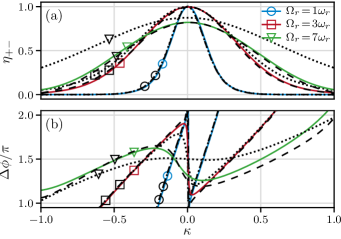
FIG. 7: Velocity dispersion of (a) the diffraction efficiency $\eta_{+-}$ and (b) the phase shift $\Delta\phi$ for sech-pulses with pulse width $\tau_{S}=\tilde{\tau}_{S\pi}$ (61) and different Rabi frequencies $\Omega_{r}=\Omega\,\omega_{2r}$. The DK-Pendellösung (67) (dotted) is suitable for $\Omega_{r}<3\,\omega_{r}$ while the extended model (76) (dashed) matches the numerical results (16) (solid) very well also for larger $\Omega_{r}$.

Adiabaticity

The crossover from the deep- to the quasi-Bragg regime at $\Omega\approx 3\,\omega_{r}$ for atomic mirrors using $\tilde{\tau}_{j\pi}$ (61) is related to the adiabaticity criterium [82]

$$\max_{\tau\in[\tau_{i},\tau_{i}+\Delta\tau]}\left|\frac{d}{d\tau}\left(\frac{\bm{g}_{n}^{o}(\tau)^{\ast}\dot{\bm{g}}_{m}^{o}(\tau)}{\omega_{n}(\tau)-\omega_{m}(\tau)}\right)\right|\Delta\tau\ll 1,$$ (77)

$\forall\,m\neq n$, with the eigenvalues $\omega_{m}(\tau)$ and eigenvectors $\bm{g}_{m}^{o}(\tau)$ of $H^{o}$ (40). Equation (77) results in $\Omega_{r}\!=\!\Omega\,\omega_{2r}\ll 4\,\omega_{r}$ for $\tilde{\tau}_{S\pi}$ at $\kappa=0$. This is confirmed by the results of Gochnauer et al. [56] and visible in Figs. 9 and 10. Therefore, while the DK-Pendellösung (67) is valid in the adiabatic regime, the extended model (76) can be even used for non-adiabatic pulses.

IV.5 Diffraction efficiency of a Gaussian pulse in the deep-Bragg limit

Due to the similarity of the Gaussian- to the sech-pulses [cf. Eqs. (47) and (50)], one can estimate the velocity selective diffraction efficiency for infinitely long Gaussian pulses in the deep-Bragg regime. The different pulses have equal nominal times (45). Therefore, approximating $\sech^{2}(a)$ from Eq. (70), with a similar exponential form, providing the same integration area as $\int_{-\infty}^{\infty}\text{d}a\sech^{2}(a)=\int_{-\infty}^{\infty}\text{d}a\exp(-\pi a^{2}/4)=2$, leads to

$$\eta_{+-}^{G}(\kappa,\Omega,T)=\exp\left(\!-\pi\Big{(}\frac{\kappa T}{4}\Big{)}^{2}\right)\sin^{2}\left(\frac{T\Omega}{2}\right).$$ (78)

The results are discussed in the next section.

IV.6 Diffraction efficiency for all pulses in (1+1)D

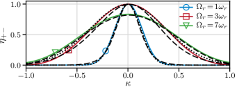
FIG. 8: Velocity dependent diffraction efficiency $\eta_{+-}(\kappa)$ for a Gaussian pulse ($j=G$, solid: numerical, dotted: deep-Bragg limit (78)) and the $\sech$ pulse [$j=S$, dashed: analytical (76)]. A mirror pulse of width $\tilde{\tau}_{j\pi}$ (61) with total pulse duration $\Delta\tau=8\tilde{\tau}_{G\pi}$ is applied for three Rabi frequencies $\Omega_{r}=\Omega\,\omega_{2r}$.

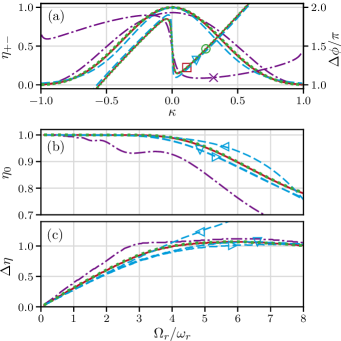
FIG. 9: Comparison of the Bragg diffraction for a mirror pulse width $\tilde{\tau}_{i\pi}$, for rectangular- (dash-dotted $\bm{\times}$), Gaussian- (solid $\bm{\square}$), Blackman- (dotted $\bm{\circ}$) and sech-pulses (dashed, numerical: $\bm{\triangledown}$, DK (67) $\bm{\triangleleft}$, DK (76) $\bm{\triangleright}$). (a) Velocity dispersion of the numerical diffraction efficiency $\eta_{+-}$ (without plotmarkers) and phase shift $\Delta\phi$ (with plotmarkers) for $\Omega_{r}=\Omega\,\omega_{2r}=3\,\mathrm{\omega_{r}}$. (b) On-resonance diffraction efficiency $\eta_{0}$ and (c) width of the diffraction efficiency $\Delta\eta$ versus $\Omega_{r}$.

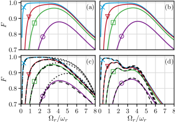
FIG. 10: Fidelity $F(\Omega_{r},\sigma_{k})$ after a mirror pulse of width $\tilde{\tau}_{i\pi}(\Omega)$ (61) versus the two-photon Rabi frequency $\Omega_{r}\!=\!\Omega\,\omega_{2r}$ for different initial atomic momentum widths $\sigma_{k}\!=\!\{0.01,0.05,0.1,0.2\}k_{L}$, {$\bm{\times}$, $\bm{\triangledown}$, $\bm{\square}$, $\bm{\circ}$}; for (a) Gaussian, (b) Blackman, (c) sech and (d) rectangular pulses. The total interaction time is $\Delta\tau=8\,\tilde{\tau}_{G\pi}$ (a-c) and $\Delta\tau=2\tilde{\tau}_{R\pi}$ (d), cf. Eq. (61). The 1D initial Gaussian wavepacket (98) is centered at $(x,k_{x})=(0,-k_{L})$. The DK-Pendellösung (67) [dotted, (c)] matches the results of the numerical integration (16) (solid) very well for $\Omega_{r}<3\,\omega_{r}$, considering population loss to higher diffraction orders (76) (dashed) also for larger $\Omega_{r}$. The Kato solution (121) (dashed) is depicted in (d), matching the numerical results.

In beamsplitter experiments, Gaussian laser pulses are ubiquitous. There is a good reason for it, as they are self-Fourier-transform functions. This is evident in the numerical simulations of first order diffraction efficiency in Fig. 8, which is free of the side lobes of rectangular pulses, seen in Fig. 6 (a). The diffraction efficiency becomes power-broadened for increasing Rabi frequency. Beyond $\Omega_{r}>3\omega_{r}$, scattering into higher diffraction order depletes the population in the beamsplitter manifold. However, in the deep-Bragg regime, the approximation (78) matches the numerical solutions very well. Sech-pulses [extended DK-model (76)] behave similarly, as shown in Fig. 8 and 9. The explicit solution for the sech-pulse [extended DK-model (76)] deviates slightly from Gaussian- and Blackman-pulses, but provides very detailed forecasts. Indeed, all smooth pulse shapes ($j=G,B,S$) with pulse widths $\tilde{\tau}_{j\pi}$ are very similar and exhibit almost identical phase shifts and efficiencies as depicted in Fig. 9. Here, for finite total interaction times $\Delta\tau$, the $\pi$-pulse conditions are not met exactly $\Omega T_{j}(-\Delta\tau/2,\Delta\tau/2)\approx\pi$ (45). One could adjust the pulse width $\tilde{\tau}_{j\pi}$ for each pulse shape $j$ to obtain a $\pi$ pulse individually $\Omega T_{j}(-\Delta\tau/2,\Delta\tau/2)=\pi$, but this leads to unequal nominal times $T_{j}\neq T$ (45) and results in significant phase differences. Thus, we consider the same $\pi$-pulse time $\Delta\tau=8\tilde{\tau}_{G\pi}$ for all pulses and the widths $\tau_{j}=\tilde{\tau}_{j\pi}$ connected via $T_{j}=T$, the resulting differences in the pulse areas $\Omega T_{j}(-\Delta\tau/2,\Delta\tau/2)$ (45) are negligible.

The phase sensitive fidelity (19) for different pulse shapes and momentum widths $\sigma_{k}$ of an initial Gaussian wavepacket in 1D (98) are compared in Fig. 10. For the smooth envelopes, an increasing $\sigma_{k}$ reduces the range of admissible Rabi frequencies $\Omega_{r}\!=\!\Omega\,\omega_{2r}$, which shifts the optimum to higher values. Evidently, the DK-Pendellösung (67) matches numerical simulations for $\Omega_{r}<3\,\mathrm{\omega_{r}}$, while the extended DK-model (76) remains further valid. The explicit Kato solution (121) matches the results for rectangular pulses very well, demonstrating its applicability for wavepackets with finite momentum width.

IV.7 Diffraction efficiency for spatial Gauss-Laguerre modes with pulse shapes in (3+1)D

IV.7.1 Gauss-Laguerre modes

The experimental beamsplitter beams are pulsed, bichromatic, counterpropagating Gauss-Laguerre modes [83]. In the specific frame $S^{\prime}$, comoving with the nodes of the interference pattern, there is only a single wavenumber $k_{L}$ (cf. (15) and Apps. A, B). The slowly varying amplitude of the electric field leads to Rabi frequencies

$$\Omega_{j}(t,\bm{r})=\Omega_{j}(t,\varrho)e^{i\Phi(\varrho)},$$ (79)

$$\Omega_{j}(t,\varrho)=\Omega_{j}(t)\frac{w_{0}}{w_{j}}e^{-\frac{\varrho^{2}}{w_{j}^{2}}},\qquad\Phi(\varrho)=\frac{k_{L}\varrho^{2}}{2R_{j}}-\xi_{j}$$ (80)

with beam parameters $w_{1,2}=w(\ell/2)$, $R_{1,2}=\pm R(\ell/2)$, $\xi_{1,2}=\pm\xi(\ell/2)$ and the distance $\ell$ between both lasers beam waists, as depicted in Fig. 11.

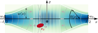
FIG. 11: Two counterpropagating, bichromatic Gauss-Laguerre beams form a travelling, standing wave (12) with an intensity pattern in cylindrical coordinates $(x,\varrho)$. The gray arrows are the local wavevectors, $w(x)$ is the local waist and $R(x)$ the local radius of curvature. The distance between the two beam waists is $\ell$. The atomic cloud, generally localized at $\bm{r}_{0}$ is indicated as red ellipse.

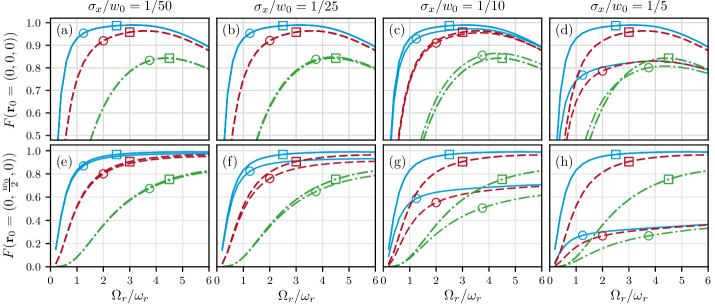
FIG. 12: Fidelity $F(\Omega_{r},\sigma_{k},\sigma_{x})$ after a mirror pulse versus two-photon Rabi frequency $\Omega_{r}=\Omega\,\omega_{2r}$ for different atomic initial momentum widths $\sigma_{k}=\{0.05,\ 0.1,\ 0.2\}\times k_{L}$, {solid blue, dashed red, dashed-dotted green} of a 3D ballistically expanded Gaussian wavepacket (100) for Gauss-Laguerre beams ($\bm{\circ}$) in comparison to plane waves ($\bm{\square}$), using the (3+1)D numerical integration (16). Gaussian temporal pulses of width $\tilde{\tau}_{G\pi}(\Omega)$ (61) and total duration $\Delta\tau=8\,\tilde{\tau}_{G\pi}$ (61) are applied. Each column represents a different ratio $\sigma_{x}/w_{0}$ between spatial width of the initial state $\sigma_{x}$ and the beam waist $w_{0}$. In the bottom row the atomic initial state is displaced in the radial direction of the Gaussian beams to $\varrho_{0}=y_{0}=w_{0}/2$.

IV.7.2 Local plane-wave approximation

To isolate the momentum kick of the beamsplitter from the momentum imparted by the dipole force, we consider a local plane-wave approximation of the Gauss-Laguerre beam at the initial position $\bm{r}_{0}=(0,\bm{\varrho}_{0})$, $\bm{\varrho}_{0}=(y_{0},z_{0})$ of the atomic cloud

$$\Omega_{j}(t,\bm{r})\approx\Omega_{j}(t,\bm{r}_{0})=\Omega_{j}(t,\varrho_{0})e^{i\Phi(\varrho_{0})}.$$ (81)

Thus, the atomic cloud feels only a reduced Rabi frequency but experiences no spatial inhomogeneity. Therefore, simulations with plane waves must be independent of the ratio $\sigma_{x}/w_{0}$ for $\sigma_{x}>\lambda$.

IV.7.3 Simulations

Beamsplitters perform best, if the atomic cloud (of size $\sigma_{x}\sim$\mathrm{\SIUnitSymbolMicro m}$-$\mathrm{mm}$$) is well localized within the beam waist $w_{0}$. For $w_{0}\sim$\mathrm{m}\mathrm{m}$$ and optical wavelengths $\lambda\sim$\mathrm{\SIUnitSymbolMicro m}$$ the Rayleigh lengths $x_{R}$ are several meters, thus

$$x_{R}\gg w_{0}>\sigma_{x}>\lambda.$$ (82)

Therefore, one can expect that the transversal dipole forces will be stronger than the forces along the propagation direction $x$. Small clouds centered at the symmetry point $\bm{r}_{0}=(0,0,0)$ will feel the least degradation of the beamsplitter fidelity [cf. Fig. 12 (a) and (b)] due to dipole forces. This will be confirmed by displacing the initial cloud transversely to $\bm{r}_{0}=(0,w_{0}/2,0)$, leading to larger aberrations [cf. Fig. 12 (e)-(h)].

In these simulations of a Bragg mirror, depicted in Fig.  12, we use the effective $\pi$-pulse width $\tilde{\tau}_{G\pi}(\Omega(\bm{r}_{0}))$ (61) in the local plane-wave approximation (81) for different Rabi frequencies $\Omega_{r}=\Omega\,\omega_{2r}$ and a longitudinal laser displacement $\ell=0.1\,x_{R}$, like in the experiment (cf. Tab. 2). As initial states of the atomic cloud, we consider ballistically expanded 3D Gaussian wavepackets (100) with different widths in real space $\sigma_{x}$ and in reciprocal space $\sigma_{k}$.

For atoms located at the center of the Gaussian laser beams, the spatial inhomogeneity (107) leads to significant aberrations only for large atomic clouds [cf. Fig. 12 (c), (d)]. By contrast, even small displaced clouds [cf. Fig. 12 (e), (f)] show a significant reduction of the fidelity in realistic Gaussian beams compared to ideal plane waves. The latter uses a reduced Rabi frequency according to the local plane-wave approximation (81). For large clouds this reduction is detrimental [cf. Fig. 12 (g), (h)]. Please note that we use parameters, where the simulation results for the fidelity only depend on the ratio $\sigma_{x}/w_{0}<1$.

Besides the phase sensitive fidelity, the aberrations due to Gaussian beams are already apparent in the diffraction efficiency. In Fig. 13 the momentum density $\tilde{n}(k_{x},k_{y})$ is shown for the (3+1)D simulation with (a) Gauss-Laguerre laser beams and (b) the idealized local plane-wave approximation, after a mirror pulse with $\Omega_{r}=3\,\mathrm{\omega_{r}}$. In the momentum space, the splitting is visible directly after the $\pi$-pulse. We study a ballistically expanded Gaussian wavepacket (100) as initial state with $\sigma_{k}=0.05\,\mathrm{k_{L}}$ and $\sigma_{x}=1/25\,w_{0}$, located at $\bm{r}_{0}=(0,w_{0}/2,0)$. The logarithmic scale highlights the imperfections of the Bragg diffraction, using Gaussian laser beams. Even for the tiny momentum width, the diffraction efficiency is reduced to $96.3\,\mathrm{\%}$ in comparison to $97.8\,\mathrm{\%}$ for idealized plane waves. In addition, the dipole force leads to a rogue, transversal momentum component $\langle\hat{p}_{y}\rangle=0.012\,\mathrm{\hbar}k_{L}$. As opposed to the diffraction efficiency and the fidelity, this momentum component depends not only on the relation $\sigma_{x}/w_{0}$ but on the beam waist, here $w_{0}=$62.5\text{\,}\mathrm{\SIUnitSymbolMicro m}$$. Further studies of the mechanical light effects of the dipole force are subjects of our present research.

Locating the initial state at the center $\bm{r}_{0}=(0,0,0)$ reduces the aberrations due to Gauss-Laguerre laser beams. The diffraction efficiency of $99.0\,\mathrm{\%}$ reaches almost the efficiency of idealized plane waves with $99.1\,\mathrm{\%}$ and the transverse momentum component vanishes.

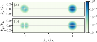
FIG. 13: Column integrated atom density in momentum space $\tilde{n}(k_{x},k_{y})=\int\text{d}k_{z}\,|\tilde{\psi}(k_{x},k_{y},k_{z})|^{2}$ after a $\pi$ pulse for (a) Gaussian laser beams and (b) plane waves. The initial state is a temporally evolved Gaussian wavepacket (100) located at $\bm{r}_{0}=(0,w_{0}/2,0)$ with momentum width $\sigma_{k}=0.05\,k_{L}$ and expansion size $\sigma_{x}=w_{0}/25=$2.5\text{\,}\mathrm{\SIUnitSymbolMicro m}$$. Gaussian pulses with $\Omega_{r}=\Omega\,\omega_{2r}=3\,\mathrm{\omega_{r}}$, $\tau_{G}=\tilde{\tau}_{G\pi}(\Omega)$ (61), $\Delta\tau=8\,\mathrm{\tilde{\tau}_{G\pi}}$ and beam waist $w_{0}=$62.5\text{\,}\mathrm{\SIUnitSymbolMicro m}$$ are applied. The final momentum expectation value in $y$-direction $\langle\hat{p}_{y}\rangle=0.012\,\mathrm{\hbar}k_{L}$ is highlighted with grey lines.

V Proving the Demkov-Kunike model experimentally

Experimentally, we employ an atom chip apparatus to Bose-condense ⁸⁷Rb [84, 34] with a condensate fraction of $N^{c}=$(10\pm 1.)\text{\times}{10}^{3}$$ and a quantum depletion (thermal cloud) of $N^{t}=$(7\pm 1.)\text{\times}{10}^{3}$$ . After release from the trap (lab frame $S$), with trap frequencies listed in Tab. 2, they expand ballistically and fall vertically towards Nadir. The Bragg-laser beams are aligned horizontally. It is sufficient to consider inertial motion during the short Bragg pulses (<$\mathrm{m}\mathrm{s}$). After $10\text{\,}\mathrm{ms}$ time-of-flight (TOF), at the beginning of the diffraction pulses, the temperature of the thermal cloud is obtained from a bimodal fit [85] as $T=$20\pm 3\text{\,}\mathrm{nK}$$. So far, the cloud $\sigma_{x}=$20\text{\,}\mathrm{\SIUnitSymbolMicro m}$$ is much smaller than the beam waist $w_{0}=$1386\text{\,}\mathrm{\SIUnitSymbolMicro m}$$ and permits the plane-wave approximation.

Experimentally, the first order diffraction efficiency in the deep-Bragg limit

$$\eta=\frac{N_{+}}{N_{-}+N_{+}}$$ (83)

is obtained from the number of atoms $N_{+}$ diffracted into the first order $k^{\prime}=k_{+}$ and the undiffracted atoms $N_{-}$ remaining in the initial state $k^{\prime}=k_{-}$. The diffraction efficiency is either a function of the detuning $\delta\omega$ (6) of the laser from the two-photon resonance with atoms initially at rest $\langle\hat{p}_{x}(\tau_{i})\rangle=0$, or it is the response for resonant lasers and an initial wavepacket centered at

$$\langle\hat{p}_{x}(\tau_{i})\rangle=(-1+\bar{\kappa})\hbar k_{L},\qquad\bar{\kappa}=\frac{\mbox{$\delta\omega$}}{\omega_{2r}},$$ (84)

using Eq. (8) (cf. Sec. II.2).

Theoretically, we compute the diffraction efficiency (83) in the laser plane-wave approximation from the number of diffracted atoms

$$N_{\pm}(\bar{\kappa})=\int_{-1}^{1}\text{d}\kappa\,\eta_{\pm-}(\kappa)\,n(\kappa,\bar{\kappa}),$$ (85)

following from a reaction equation derived in App. E, which completely encloses the wavepacket with the effectively one-dimensional momentum density $n(\kappa,\bar{\kappa})$ and the average initial momentum $\bar{\kappa}$. Please note that for ideal plane matter-waves with wavenumber $\bar{\kappa}$ the diffraction efficiency (83) reduces to $\eta=\eta_{+-}(\bar{\kappa})$. In the deep-Bragg regime, theoretically $N_{+}+N_{-}=N^{A}=N^{c}+N^{t}$ and the diffraction efficiency simplifies to

$$\eta=\frac{N_{+}(\bar{\kappa})}{N^{A}}=p^{c}\mathfrak{n}_{+}^{c}(\bar{\kappa})+p^{t}\mathfrak{n}_{+}^{t}(\bar{\kappa}),$$ (86)

splitting into a condensate and a thermal cloud fraction with $p^{c}=N^{c}/N^{A}$, $p^{t}=1-p^{c}$. Approximating the normalized initial momentum distributions $\mathfrak{n}^{c}(\kappa,\bar{\kappa})$, $\mathfrak{n}^{t}(\kappa,\bar{\kappa})$ by Gaussian functions (141) of widths $\sigma_{k}^{c}=0.087\,k_{L}$ and $\sigma_{k}^{t}=(0.237\pm 0.015)\,k_{L}$ (cf. App. E.1) and using the Gaussian approximation (78) for the diffraction efficiency $\eta_{\pm-}(\kappa)$, one obtains the analytical model

$$\eta=\sin^{2}\left(\frac{\Omega T}{2}\right)\sum_{a=\{c,{t}\}}\frac{p^{a}}{\tilde{\sigma}_{k}^{a}(\tilde{T})}e^{-\frac{(\bar{\kappa}\tilde{T})^{2}}{2\tilde{\sigma}_{k}^{a}(\tilde{T})^{2}}},$$ (87)

with $\tilde{\sigma}_{k}^{a}(\tilde{T})=\sqrt{1+(\tilde{T}\tilde{\sigma}_{k}^{a})^{2}}$, $\tilde{T}=T\sqrt{\pi/8}$, $\sigma_{k}^{a}=\tilde{\sigma}_{k}^{a}k_{L}$.

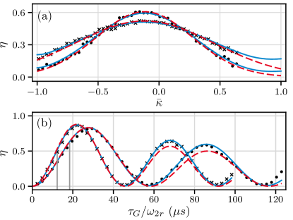
FIG. 14: Experimental diffraction efficiency $\eta$ (83) for different laser powers $P_{\bullet}=20\,\mathrm{mW}$ and $P_{\bm{\times}}=30\,\mathrm{mW}$ of Gaussian pulses of width $\tau_{G}$ with numerical simulations (solid, blue) and fits (87) (dashed, red) based on the DK-model. (a) Velocity selectivity for $\Omega T_{G}=0.56\,\mathrm{\pi}$ pulses (45) versus detuning $\bar{\kappa}$ of the initial central momentum$\langle\hat{p}_{x}(\tau_{i})\rangle=(-1+\bar{\kappa}^{S}+\bar{\kappa})\hbar k_{L}$, were $\bar{\kappa}^{S}k_{L}=0.12\,k_{L}$ is a small initial velocity of the atoms in the lab frame $S$ and $\bar{\kappa}=\mbox{$\delta\omega$}/\omega_{2r}$ (8). (b) Rabi oscillations of the diffraction efficiency versus pulse width $\tau_{G}$, with total interaction time $\Delta\tau=8\tau_{G}$ and highlighted pulse widths of (a). Other parameters cf. Tab. 1, 2.

In Fig. 14, the diffraction efficiency (83) is depicted for two different laser powers $P_{\bullet}=$20\text{\,}\mathrm{mW}$$, $P_{\bm{\times}}=$30\text{\,}\mathrm{mW}$$ of a Gaussian pulse of width $\tau_{G}$ (47) and total interaction time $\Delta\tau=8\tau_{G}$. In the experiment, the atoms are displaced axially to $z_{0}=$1165\pm 50.\text{\,}\mathrm{\SIUnitSymbolMicro m}$=($0.84\pm 0.04$)w_{0}$, while $x_{0}=y_{0}=$0\text{\,}\mathrm{\SIUnitSymbolMicro m}$$. This reduces the effective Rabi frequency at the location of the atoms (81).

Fits using the model (87) describe the experimental data already very well and provide starting parameters [$p_{c}$, $\Omega(\bm{r}_{0})$] for the effective (1+1)D numerical simulations with Gaussian pulses, fully matching the experimental data. The experimental, numerical and fit parameters are listed in Tab. 1.

In Fig. 14 (a), the velocity dispersion of the diffraction efficiency uncovers an initial motion $k_{x}^{S}=\bar{\kappa}^{S}k_{L}=0.12\,k_{L}$ of the atomic cloud in the lab frame $S$. Considering this in $\langle\hat{p}_{x}(\tau_{i})\rangle=(-1+\bar{\kappa}^{S}+\bar{\kappa})\hbar k_{L}$ with $\bar{\kappa}=\mbox{$\delta\omega$}/\omega_{2r}$ leads to a very good match of the fit model (87), the simulations and the experimental data.

In Fig. 14 (b), the diffraction efficiency displays damped Rabi oscillations versus the pulse width $\tau_{G}$. This is a typical inhomogeneous line-broadening caused by the momentum widths $\sigma_{k}^{c}$, $\sigma_{k}^{th}$, the two-photon detuning $\mbox{$\delta\omega$}=\bar{\kappa}\omega_{2r}\neq 0$ and a residual velocity $\bar{\kappa}^{S}\neq 0$. It is also revealed by the Gaussian approximation (87). The fit results for the two-photon Rabi frequency are also optimal for the numerical simulations matching the experiment within the error level.

Table 1: Parameters of Fig. 14 for the experiment (e), the numerical simulation (n) and the approximation (87) (a).

			$P_{\bullet}\negmedspace=\negmedspace$20\pm 2.\text{\,}\mathrm{m}\mathrm{W}$$	$P_{\bm{\times}}\negmedspace=\negmedspace$30\pm 3.\text{\,}\mathrm{m}\mathrm{W}$$
	e	$p_{c}$	$0.59\pm 0.08$	$0.59\pm 0.08$
	e	$\Omega$	$6.60\pm 0.66\text{\,}\omega_{\mathrm{r}}$	$9.89\pm 0.99\text{\,}\omega_{\mathrm{r}}$
	e	$\Omega(\bm{r}_{0})$	$1.61\pm 0.27\text{\,}\omega_{\mathrm{r}}$	$2.41\pm 0.40\text{\,}\omega_{\mathrm{r}}$
	e	$\bar{\kappa}^{S}k_{L}$	$(0.12\pm 0.01)\,k_{L}$	$(0.12\pm 0.01)\,k_{L}$
(a)	e	$\tau_{G}/\omega_{2r}$	$147.45\,\mathrm{\mu s}$	$98.3\,\mathrm{\mu s}$
	e	$\Omega(\bm{r}_{0})T_{G}$ (45)	$0.56\,\mathrm{\pi}$	$0.56\,\mathrm{\pi}$
	a	$p_{c}$	$0.59\pm 0.06$	$0.59\pm 0.14$
	a	$\Omega(\bm{r}_{0})$	$(1.74\pm 0.01)\,\omega_{r}$	$(2.27\pm 0.01)\,\omega_{r}$
	n	$p_{c}$	$0.59$	$0.59$
	n	$\Omega(\bm{r}_{0})$	$1.71\,\omega_{r}$	$2.28\,\mathrm{\omega_{r}}$
(b)	e	$\mbox{$\delta\omega$}/2\pi$	$-2\,\mathrm{kHz}$	$-2.5\,\mathrm{kHz}$
	a	$p_{c}$	$0.55\pm 0.03$	$0.59\pm 0.04$
	a	$\Omega(\bm{r}_{0})$	$(1.81\pm 0.01)\,\omega_{r}$	$(2.30\pm 0.01)\,\omega_{r}$
	n	$p_{c}$	$0.52$	$0.52$
	n	$\Omega(\bm{r}_{0})$	$1.81\,\omega_{r}$	$2.30\,\omega_{r}$

It is worth mentioning that the velocity dispersion of the efficiency [Fig. 14 (a)] is less sensitive to the condensate ratio $p^{c}$ than the Rabi oscillations [Fig. 14 (b)]. The Gaussian approximation (87) underestimates the second maxima, but the fit of $p^{c}$ matches the experimental value within its uncertainty. The numerical simulations predict a condensate ratio at the lower bound of the experimental ratio, still within the uncertainty. The reduction of condensate fraction $p^{c}$ in simulations and Gaussian approximation is equivalent to increasing the momentum width of the condensate or thermal cloud.

Thus, the Gaussian approximation (87) of the DK-model gives an unbiased prediction of the experimental data. It assumes weak two-photon Rabi frequencies $\Omega_{r}(\bm{r}_{0})<3\,\omega_{r}$, justifying the Pendellösung (70) and small atomic clouds $\sigma_{x}\ll w_{0}$ to approximate Gaussian beams by plane-waves.

VI Conclusion

We present (3+1)D simulations and analytical models of a pulsed atomic Bragg beamsplitter. Thereby, we characterize ubiquitous imperfections, like the velocity dispersion and the population losses into higher diffraction orders. We study the influence of four common temporal pulses (rectangular-, Gaussian-, Blackman- and hyperbolic sech pulse). Clearly, the diffraction efficiency and the fidelity benefit from Fourier-limited, smooth envelopes. Much insight is gained from the analytical Demkov-Kunike model for a hyperbolic secant pulse (67). It reveals the explicit dependence on the multitude of physical parameters. Due to its similarity with a Gaussian pulse, the diffraction efficiency (70) can also be used for it (78). For a large parameter regime, the model is verified experimentally and matches the velocity dispersion. The extended DK-model (76) matches also losses into higher diffraction orders.

For a rectangular pulse, we have obtained explicit higher order diffraction results from Kato degenerate perturbation theory, which provide insight in the quasi-Bragg regime. Due to a renormalization of the effective Rabi frequency in the beamsplitter manifold, one finds significant stretching of the optimal $\pi$-pulse time, which has been seen experimentally [56]. We find this stretching for all considered pulses in the quasi-Bragg regime and assume it is universal.

Comparing Gauss-Laguerre beams with plane waves reduces the diffraction efficiency and transfer fidelity, in general. The beam inhomogeneity becomes relevant for $\sigma_{x}>w_{0}/10$. But even for smaller decentered clouds, the fidelity suffers significantly. Currently, we investigate the aberrations due to laser misalignment and transversal confinement, which will be reported elsewhere.

Appendix A Comoving rotating frame

In quantum mechanics, a Galilean transformation is represented by the displacement operator [86]

$$\hat{G}(t)=e^{\frac{i}{\hbar}(\bm{\mathfrak{p}}\hat{\bm{r}}-\bm{\mathfrak{r}}(t)\hat{\bm{p}})}=e^{-\frac{i}{2\hbar}\bm{\mathfrak{p}}\bm{\mathfrak{r}}(t)}e^{\frac{i}{\hbar}\bm{\mathfrak{p}}\hat{\bm{r}}}e^{-\frac{i}{\hbar}\bm{\mathfrak{r}}(t)\hat{\bm{p}}}$$ (88)

with a time-dependent coordinate $\bm{\mathfrak{r}}(t)=\bm{\mathfrak{r}}_{0}+\bm{v}t$ and a momentum $\bm{\mathfrak{p}}=m\bm{v}$. It transforms the corresponding Heisenberg operators as

$$\begin{pmatrix}\hat{\bm{r}}^{\prime}\\ \hat{\bm{p}}^{\prime}\end{pmatrix}=\hat{G}\begin{pmatrix}\hat{\bm{r}}\\ \hat{\bm{p}}\end{pmatrix}\hat{G}^{\dagger}=\begin{pmatrix}\hat{\bm{r}}-\bm{\mathfrak{r}}(t)\\ \hat{\bm{p}}-\bm{\mathfrak{p}}\end{pmatrix}.$$ (89)

In the Schrödinger picture, $\hat{G}(t)$ transforms the lab frame state $\ket{\psi(t)}=\hat{G}(t)\ket{\psi^{\prime}(t)}$ into the state $\ket{\psi^{\prime}(t)}$ of the comoving frame. Evaluating the comoving-frame Hamilton operator $\hat{H}^{\prime}$ the Schrödinger equation reads

$$i\hbar\partial_{t}\ket{\psi^{\prime}}=\hat{H}\textquoteright\ket{\psi^{\prime}}=\hat{G}^{\dagger}(\hat{H}-i\hbar\partial_{t})\hat{G}\ket{\psi^{\prime}},$$ (90)

$$\hat{H}^{\prime}=\frac{\hat{\bm{p}}^{2}}{2M}+\hbar\omega_{g}\hat{\sigma}_{g}+\hbar\omega_{e}\hat{\sigma}_{e}+V(t,\hat{\bm{r}}+\bm{\mathfrak{r}}(t)).$$ (91)

In the frame, moving with the group velocity $\bm{v}=v_{g}\bm{e}_{x}$ (12) in the x-direction, the Doppler shifted laser phases

$$\phi^{\prime}_{1} =\omega_{1}t-k_{1}(\hat{x}+\mathfrak{x}_{0}+v_{g}t)=\omega_{L}t-k_{1}(\hat{x}+\mathfrak{x}_{0}),$$ (92)

$$\phi^{\prime}_{2} =\omega_{2}t+k_{2}(\hat{x}+\mathfrak{x}_{0}+v_{g}t)=\omega_{L}t+k_{2}(\hat{x}+\mathfrak{x}_{0})$$ (93)

oscillate synchronously with

$$\omega_{L}=\frac{\omega_{1}+\omega_{2}}{2}\left(1-\beta^{2}\right)\approx\frac{\omega_{1}+\omega_{2}}{2}.$$ (94)

The second order correction in $\beta=v_{g}/c$ can be neglected safely in our nonrelativistic scenario.

Another local frame transformation $\ket{\psi^{\prime}}=\hat{F}\ket{\psi^{\prime\prime}}$, eliminates the rapid temporal oscillations and establishes a single spatial period $\lambda=2\pi/k_{L}$ of the optical potential

$$\hat{F}(t)=e^{-i\omega_{g}t-i\omega_{L}t\hat{\sigma}_{e}+\frac{i}{2}[k_{12}(\hat{x}+\mathfrak{x}_{0})-\chi_{12}]\hat{\sigma}_{z}}.$$ (95)

Now, the transformed Schrödinger equation reads

$$\begin{split}&i\hbar\partial_{t}\ket{\psi^{\prime\prime}}=\hat{H}^{\prime\prime}\ket{\psi^{\prime\prime}},\end{split}$$ (96)

$$\begin{split}&\hat{H}^{\prime\prime}=\frac{(\hat{p}_{x}+\tfrac{1}{2}\hbar k_{12}\hat{\sigma}_{z})^{2}}{2M}+\frac{\hat{p}^{2}_{y}+\hat{p}^{2}_{z}}{2M}-\hbar\Delta\hat{\sigma}_{e}\\ &\phantom{+}+\frac{\hbar}{2}\hat{\sigma}^{\dagger}\left(\tilde{\Omega}_{1}(t,\hat{\bm{r}})e^{ik_{L}\hat{x}}+\tilde{\Omega}_{2}(t,\hat{\bm{r}})e^{-ik_{L}\hat{x}}\right)+\text{h.c.}\end{split}$$ (97)

with a laser detuning $\Delta=\omega_{L}-\omega_{0}$, a common wavenumber $k_{L}=(k_{1}+k_{2})/2$ and a relative wavenumber mismatch $k_{12}=(k_{1}-k_{2})/2$. Global phases of the Rabi frequencies $\Omega_{i}(t,\bm{r})=\tilde{\Omega}_{i}(t,\bm{r})e^{-i\chi_{i}}$ do vanish with the proper gauge $\chi_{12}=(\chi_{1}+\chi_{2})/2$ and the shifted coordinate origin $\mathfrak{x}_{0}=(\chi_{1}-\chi_{2})/2k_{L}$.

Please note, $k_{12}=(\omega_{1}-\omega_{2})/c\sim$1\text{\times}{10}^{-10}\text{\,}\mathrm{\SIUnitSymbolMicro}\mathrm{m}^{-1}$\sim$1\text{\times}{10}^{-11}\text{\,}\,$k_{L}$ is tiny in comparison to other relevant momenta. We will consider Bose-Einstein condensates with Thomas-Fermi radii in the trap of a few microns (cf. Sec. V and E.1), the momentum width can be approximated with the Heisenberg width $\Delta k_{\text{TF}}^{\text{H}}=3/2r_{\text{TF}}=$0.15\text{\,}\mathrm{\SIUnitSymbolMicro}\mathrm{m}^{-1}$$, considering $r_{\text{TF}}=$10\text{\,}\mathrm{\SIUnitSymbolMicro m}$$, while the Rayleigh width gives $\Delta k_{\text{TF}}^{\text{R}}=$0.51\text{\,}\mathrm{\SIUnitSymbolMicro}\mathrm{m}^{-1}$$ [87]. In our simulations, we consider atomic initial states as Gaussian wavepackets with momentum widths $\sigma_{k}\in[0.01,0.05,0.1,0.2]\,k_{L}$, with $k_{L}\approx$8\text{\,}\mathrm{\SIUnitSymbolMicro}\mathrm{m}^{-1}$$, to compare $\Delta k_{\text{TF}}^{\text{R}}$ corresponds to $\sigma_{k}^{\text{R}}\approx\Delta k_{\text{TF}}^{\text{R}}/3=0.02\,k_{L}$. After release out of the trap the momentum width of the BEC increases. With temperatures $T\leq$20\text{\,}\mathrm{nK}$$ this gives rise for momentum widths of a thermal cloud $\sigma_{k}=\sqrt{k_{B}TM}/\hbar\leq$0.23\text{\,}\,$k_{L}$. Therefore, $k_{12}$ can be neglected safely.

Appendix B Spreading Gaussian waves

Matter waves

Ballistically spreading Gaussian wavepackets are useful input states to test a beamsplitter. Using different expansion times $t$, one can vary the position width $\sigma_{x}$, while keeping the momentum width $\sigma_{k}$ constant. A $n$-dimensional Gaussian unnormalized wavepacket is defined as

$$\psi_{0}(\bm{r})=e^{i\bm{k}_{0}(\bm{r}-\bm{r}_{0})-\frac{1}{2}(\bm{r}-\bm{r}_{0})(2\Sigma_{0})^{-1}(\bm{r}-\bm{r}_{0})}$$ (98)

$$=\int\frac{\text{d}^{n}k}{(2\pi)^{\frac{n}{2}}}e^{i\bm{k}\bm{r}}\sqrt{|2\Sigma_{0}|}e^{-i\bm{k}\bm{r}_{0}-\frac{1}{2}(\bm{k}-\bm{k}_{0})(2\Sigma_{0})(\bm{k}-\bm{k}_{0})}$$

and centered at $(\bm{r}_{0},\bm{k}_{0})=(\langle\bm{r}\rangle,\langle-i\nabla\rangle)$. The wavepacket is normalized to $\int\text{d}^{n}r\,|\psi_{0}|^{2}=\sqrt{|2\pi\Sigma_{0}|}$ with the covariance matrix $\Sigma_{0}=\langle(\bm{r}-\bm{r}_{0})\otimes(\bm{r}-\bm{r}_{0})\rangle$. The three dimensional free Schrödinger equation

$$i\partial_{t}\psi(t,\bm{r})=-\frac{\alpha}{2}\Delta_{r}\psi,\qquad\alpha=\frac{\hbar}{M}$$ (99)

describes the spreading of a matter-wave using the Fourier-transformed field $\tilde{\psi}_{0}(\bm{k})$ implicitly defined in (98)

$$\psi(t,\bm{r})=\int\frac{\text{d}^{n}k}{(2\pi)^{\frac{n}{2}}}e^{-it\frac{\alpha}{2}k^{2}}e^{i\bm{k}\bm{r}}\tilde{\psi}_{0}(\bm{k})$$ (100)

$$=\mathcal{A}(t)e^{-i\Theta(t)}e^{i\bm{k}_{0}[\bm{r}-\bm{r}_{0}]-\frac{1}{2}[\bm{r}-\bm{r}_{0}(t)][2\Sigma(t)]^{-1}[\bm{r}-\bm{r}_{0}(t)]}.$$

The evolving center position $\bm{r}_{0}(t)$, spreading covariance $\Sigma(t)$, dynamical phase $\Theta(t)$ and scale-factor $\mathcal{A}(t)$ read

$$\Sigma(t) =\Sigma_{0}+it\frac{\alpha}{2}, \bm{r}_{0}(t) =\bm{r}_{0}+t\alpha\bm{k}_{0},$$ (101)

$$\Theta(t) =t\frac{\alpha k_{0}^{2}}{2}, \mathcal{A}(t) =\sqrt{\frac{|\Sigma_{0}|}{|\Sigma(t)|}}.$$ (102)

In the simulations, we assume an isotropic initial state with $\Sigma_{ij}=\delta_{ij}\sigma_{x}^{2}$ and

$$\sigma_{x}(t)=\sigma_{x}\sqrt{1+(t/t_{H})^{2}},$$ (103)

with the Heisenberg time $t_{H}=2\sigma_{x}^{2}M/\hbar$.

Gaussian laser beams

The scalar mode of a circularly symmetric Gauss-Laguerre beam propagating along the x-direction follows from the two-dimensional $n=2$ paraxial approximation of the Helmholtz equation

$$i\partial_{x}u(x,\bm{\varrho})=-\frac{\beta}{2}\Delta_{\varrho}u,\qquad\beta=k_{L}^{-1},\quad\bm{\varrho}=(y,z).$$ (104)

The spatially evolved mode $u(x,\bm{\varrho})$ follows analogously from (100), (101), substituting $(t,\alpha)\leftrightarrow(x,\beta)$

$$u(x,\bm{\varrho})=\frac{x_{R}}{iq(x)}e^{i\frac{k_{L}\varrho^{2}}{2q(x)}}=Ue^{i\Phi}$$ (105)

$$U(x,\varrho)=\frac{w_{0}}{w(x)}e^{-\frac{\varrho^{2}}{w(x)^{2}}},\quad\Phi(x,\varrho)=\frac{k_{L}\varrho^{2}}{2R(x)}-\xi(x),$$

where $\varrho=\sqrt{y^{2}+z^{2}}$ is the normal distance to the symmetry axis and $q(x)=x-ix_{R}$ is the complex beam parameter [83]. It is characterized by the Rayleigh range $x_{R}=\pi w_{0}^{2}/\lambda$, the beam waist $w(x)=w_{0}(1+(x/x_{R})^{2})^{1/2}$, the minimum waist $w_{0}=2\sigma$, the radius of wavefront curvature $R(x)=x(1+(x_{R}/x)^{2})$, the Gouy phase $\xi=\arctan(x/x_{R})$ and the wavelength $\lambda_{L}=2\pi/k_{L}$.

We consider two counterpropagating Gaussian laser beams, which are symmetrically displaced with respect to their waists by a distance $\ell$. Then, the dipole interaction energy in the comoving, rotating frame (LABEL:eq:hamtrafoII), reads

$$\hat{V}^{\prime\prime}=\frac{\hbar}{2}\hat{\sigma}^{\dagger}\left[\Omega_{1}(t,\bm{r})e^{ik_{L}x}+\Omega_{2}(t,\bm{r})e^{-ik_{L}x}\right]+\text{h.c.},$$ (106)

with pulse amplitudes $\Omega_{j}(t)$ and spatial envelopes

$$\Omega_{j}(t,\bm{r})=\Omega_{j}(t)U(x_{j},\varrho)e^{i\Phi(x_{j},\varrho)}.$$ (107)

We use shifted coordinates $x_{1/2}=\pm(x+v_{g}t+\ell/2)$ and beam parameters $w_{j}=w(x_{j})$, $R_{j}=R(x_{j})$ and $\xi_{j}=\xi(x_{j})$, which are slowly varying for $x\ll x_{R}$. Beamsplitter pulses are typical short and one can neglect the ballistic displacement $v_{g}t\sim$\mathrm{\SIUnitSymbolMicro m}$\ll\ell,x_{R}$. For small atomic clouds $\sigma_{x}<w_{0}/3$, one can approximate $x_{1}\approx-x_{2}\approx\ell/2$.

Appendix C Degenerate perturbation theory

To rectify the Pendellösung (54) with contributions from higher order diffraction, we employ Kato’s method for the stationary eigenvalue problem in the presence of degeneracy [79]. All eigenvalues of the diagonal part $D_{0}=D(\kappa=0)$ of the Bragg Hamilton operator (42) are doubly degenerated $1\leq\alpha\leq 2$ on resonance. Therefore, we consider the flow of the eigensystem $\mathcal{H}(\lambda)\mathbf{v}_{i,\alpha}(\lambda)=\omega_{i,\alpha}(\lambda)\mathbf{v}_{i,\alpha}(\lambda)$ with

$$\mathcal{H}=D_{0}+\lambda\mathcal{V},\qquad\mathcal{V}=D(\kappa)-D_{0}+L+L^{\dagger},$$ (108)

for $0\leq\lambda\leq 1$ in the degenerate subspace $\mathcal{E}_{i}$. If we denote the orthonormal eigenvectors of $D_{0}$ with $\mathbf{v}_{i,\alpha}^{(0)}$ and their eigenvalues $\omega_{i}^{(0)}$, the eigenvectors of the interacting Hamilton operator $\mathcal{H}_{i}(\lambda)$ restricted to the subspace $\mathcal{E}_{i}$, are $\mathbf{v}_{i,\alpha}(\lambda)=P_{i}(\lambda)\mathbf{v}_{i,\alpha}^{(0)}$. Now, all efforts are put in the perturbative evaluation of the projection operator $P_{i}(\lambda)$, which evolves from the unperturbed projection $P_{i}^{(0)}$. This results in the generalized eigenvalue problem

$$\mathcal{H}_{i}\mathbf{v}_{i,\alpha}^{(0)}=\omega_{i,\alpha}K_{i}\mathbf{v}_{i,\alpha}^{(0)},$$ (109)

$$\mathcal{H}_{i}=P_{i}^{(0)}\mathcal{H}P_{i}P_{i}^{(0)},\quad K_{i}=P_{i}^{(0)}P_{i}P_{i}^{(0)},$$ (110)

with power series expressions for the operators

$$P_{i}(\lambda) =P_{i}^{(0)}+\sum_{n=1}^{\infty}\lambda^{n}A_{i}^{(n)},$$ (111)

$$A_{i}^{(n)} =-\sum_{(n)}S_{i}^{(k_{1})}\mathcal{V}S_{i}^{(k_{2})}\mathcal{V}\dots\mathcal{V}S_{i}^{(k_{n+1})},$$ (112)

$$\mathcal{H}P_{i}(\lambda) =\omega^{(0)}_{i}P_{i}(\lambda)+\sum_{n=1}^{\infty}\lambda^{n}B_{i}^{(n)},$$ (113)

$$B_{i}^{(n)} =\sum_{(n-1)}S_{i}^{(k_{1})}\mathcal{V}S_{i}^{(k_{2})}\mathcal{V}\dots\mathcal{V}S_{i}^{(k_{n+1})}.$$ (114)

Here $\sum_{(n)}$ denotes a sum over all combinations of integers $k_{i}\in\mathbb{N}_{0}$ satisfying $k_{1}+k_{2}+\ldots+k_{n+1}=n$ and

$$\vspace{-1mm}S_{i}^{(0)}=-P_{i}^{(0)},\ S_{i}^{(k>0)}=(S_{i})^{k},\,S_{i}=\frac{\mathds{1}-P_{i}^{(0)}}{\omega_{i}^{(0)}\mathds{1}-D_{0}}.$$ (115)

It is straight forward to evaluate $\mathcal{H}_{i}$ and $\mathcal{K}_{i}$ from (110) for the ground-state manifold $i=1$ to order $\mathcal{O}(\lambda^{n})$. We find that a third order truncation of the series

$$\mathcal{H}_{1} =\begin{pmatrix}0&\frac{\Omega}{2}\\ \frac{\Omega}{2}&\kappa\end{pmatrix}-2\mathcal{I}\begin{pmatrix}1&0\\ 0&1\end{pmatrix}-\mathcal{I}\begin{pmatrix}\kappa&\Omega\\ \Omega&0\end{pmatrix},$$ (116)

$$K_{1} =(1-\mathcal{I})\begin{pmatrix}1&0\\ 0&1\end{pmatrix}-\mathcal{I}\begin{pmatrix}\kappa&\frac{\Omega}{2}\\ \frac{\Omega}{2}&-\kappa\end{pmatrix},\quad\mathcal{I}=\frac{\Omega^{2}}{16}$$

agrees very good with the numerical results. The roots of the characteristic equation $|\mathcal{H}_{1}-(\omega_{1}-\omega_{1}^{(0)})K_{1}|=0$, determine the corrected eigenfrequencies of the Pendelösung. As the frequency shifts $\omega_{1}(\lambda)-\omega_{1}^{(0)}$, are already $\mathcal{O}(\lambda)$, it is consistent to use a lower approximation for $K_{1}$, which leads to better results at the specified order. In particular, we have evaluated $\tilde{\mathcal{H}}_{1}=K_{1}^{-1}\mathcal{H}_{1}$ and Taylor expanded it at the specified order

$$\tilde{\mathcal{H}}_{1}=\begin{pmatrix}-\mathcal{I}(2+\kappa)&\frac{\Omega}{2}(1-\mathcal{I})\\ \frac{\Omega}{2}(1-\mathcal{I})&\kappa-\mathcal{I}(2-\kappa)\end{pmatrix}+\order{\lambda^{4}}.$$ (117)

This leads to the succinct expression for the eigenvalues and -vectors

$$\omega_{1,\pm}=\frac{\kappa}{2}-2\mathcal{I}\pm\frac{\tilde{\Omega}}{2},\quad\mathbf{v}_{1,\pm}^{(0)}=\begin{pmatrix}2(\mathcal{I}-1)\sqrt{\mathcal{I}}\\ -\tfrac{1}{2}\kappa(1+2\mathcal{I})\pm\tilde{\Omega}\end{pmatrix},$$

$$\tilde{\Omega}=\sqrt{\kappa^{2}(1+2\mathcal{I})^{2}+\Omega^{2}(1-\mathcal{I})^{2}}$$ (118)

in terms of a corrected Rabi frequency $\tilde{\Omega}$ (59).

Analogous to that the eigenvalues of the next subspace, coupling $\mu=\pm 3$ and representing the most important loss channel, can be calculated from $\tilde{\mathcal{H}}_{3}=K_{3}^{-1}\mathcal{H}_{3}$

$$\tilde{\mathcal{H}}_{3}=\begin{pmatrix}2(1+\mathcal{I})-\kappa&0\\ 0&2(1+\mathcal{I})+2\kappa\end{pmatrix}+\order{\lambda^{3}},$$ (119)

skipping the $\lambda^{3}$ terms, which overestimate the losses into $\mu=\pm 3$. Including higher expansion orders would correct this, but we find that the lower expansion (119) is sufficient. The eigenvalues and -vectors of $\tilde{\mathcal{H}}_{3}$ are

$$\omega_{3,\pm}=2(1+\mathcal{I})+\frac{\kappa}{2}\pm\frac{3\kappa}{2},\qquad(\mathbf{v}_{3,+}^{(0)},\mathbf{v}_{3,-}^{(0)})=\mathds{1}_{2}.$$ (120)

With the eigenvectors $\mathbf{v}_{i,j}=P_{i}\mathbf{v}_{i,j}^{(0)}$, defined by the projections (111), also expanded up to $\lambda^{3}$ for $\mu=\pm 1$ and $\lambda^{2}$ for $\mu=\pm 3$, the time-dependent solution of the Schrö- dinger equation with the Hamiltonian (108) results in

$$\bm{g}^{K}(\tau) =\frac{\tilde{\bm{g}}^{K}(\tau)}{|\tilde{\bm{g}}^{K}(\tau)|^{2}},$$ (121)

$$\tilde{\bm{g}}^{K}(\tau) =\sum_{i=\{1,3\}}\sum_{j=\{+,-\}}c_{i,j}e^{-i\omega_{i,j}(\tau-\tau_{i})}\mathbf{v}_{i,j},$$ (122)

where the integration constants $c_{i}^{(j)}$ are defined by the initial condition $\tilde{\bm{g}}^{K}(\tau)=(0,1,0,0)$.

The population of the $\mu=1$ state is of special interest, because it defines the diffraction efficiency $\eta_{+-}$. On resonance ($\kappa=0$), already $\tilde{\bm{g}}^{K}(\tau)$ is approximately normalized. Therefore, it can be approximated

$$\eta_{0}^{K}(\tau)\approx|\left(\tilde{\bm{g}}^{K}(\tau)\right)_{3}|^{2}$$ (123)

$$=A\left(1+B\cos[4\tau^{\prime}(\mathcal{I}-1)\sqrt{\mathcal{I}}]+C\cos\theta_{+}+D\cos\theta_{-}\right)\!,$$

with $\theta_{\pm}=2\tau^{\prime}(1\pm\sqrt{\mathcal{I}}+2\mathcal{I}-\mathcal{I}^{3/2})$, $\tau^{\prime}=\tau-\tau_{i}$ and coefficients expanded up to the suited order $\order{\mathcal{I}^{2}}$

$$A =\frac{1}{2}-\mathcal{I}-\frac{\mathcal{I}^{2}}{2}+\order{\mathcal{I}^{3}},\quad B=-1+\order{\mathcal{I}^{3}},$$ (124)

$$C =-D=-4\mathcal{I}^{3/2}+\mathcal{O}(\mathcal{I}^{5/2}).$$

After the effective $\pi$-pulse time $\tilde{\tau}_{R\pi}=\pi/[2|\Omega|(1-\mathcal{I})]$ (61) the diffraction efficiency (123) results in Eq. (62).

Appendix D Demkov-Kunike model

The retarded Green’s function is defined as

$$G(\tau,\tau_{i})=\mathcal{T}e^{-i\int^{\tau}_{\tau_{i}}\text{d}t\,\mathcal{H}(t)}\theta(\tau-\tau_{i}),$$ (125)

$$[i\partial_{\tau}-\mathcal{H}(\tau)]G(\tau,\tau_{i})=i\delta(\tau-\tau_{i}),$$ (126)

which hold equally for the free evolution $G_{0}(\tau,\tau_{i})$ by substituting $\mathcal{H}\rightarrow\mathcal{H}_{0}$. This leads to the Dyson-Schwinger integral equation

$$G(\tau,\tau_{i})=G_{0}-i\int^{\infty}_{-\infty}\text{d}t\,G_{0}(\tau,t^{\prime})\mathcal{H}_{1}(t^{\prime})G(t^{\prime},\tau_{i}),$$ (127)

which is central to time-dependent perturbation theory.

The two-dimensional Green’s function $G_{\mp}$ of the DK-model can be expressed completely for $\Omega,\kappa\neq 0$ with the hypergeometric basis functions $f_{1},f_{2}$ form Eq. (64)

$$G_{\mp}(\tau,\tau_{i})=M(z)S(z)S^{-1}(z_{i})M^{-1}(z_{i}),$$ (128)

$$M=\begin{pmatrix}1&0\\ 0&\frac{i}{a}\sqrt{z(1-z)}\end{pmatrix},\quad S=\begin{pmatrix}f_{1}&f_{2}\\ f_{1}^{\prime}&f_{2}^{\prime}\end{pmatrix}.$$ (129)

In the important case of exact resonance $\kappa=0$, further simplifications are possible and lead to

$$G_{\mp}(\tau,\tau_{i})=\begin{pmatrix}\cos{\Delta\varphi}&-i\sin{\Delta\varphi}\\ -i\sin{\Delta\varphi}&\cos{\Delta\varphi}\end{pmatrix},$$ (130)

$$\varphi(z)=\Omega\tau_{S}\arcsin{\sqrt{z}},\qquad\Delta\varphi=\varphi(z)-\varphi(z_{i}).$$ (131)

The integrals (127) can be solved approximately analytically. However, the expressions are bulky, why we forgo showing them [81].

Appendix E Diffraction efficiency for partially coherent bosonic fields

The bosonic amplitude $\hat{a}_{g}(\mathbf{k})$ describes the ground state atoms in momentum space and obeys the commutation relation $[\hat{a}_{g}^{\phantom{\dagger}}(\mathbf{k}),\hat{a}_{g}^{\dagger}(\mathbf{q})]=\delta(\mathbf{k}-\mathbf{q})$. For a Bose-condesed sample, the single-particle density matrix

$$\rho(\mathbf{k},\mathbf{q})\equiv\langle\hat{a}_{g}^{\dagger}(\mathbf{q})\hat{a}_{g}(\mathbf{k})\rangle=\rho^{c}(\mathbf{k},\mathbf{q})+\rho^{t}(\mathbf{k},\mathbf{q}),$$ (132)

separates into a condensate $\rho^{c}(\mathbf{k},\mathbf{q})=\alpha^{\ast}(\mathbf{q})\alpha(\mathbf{k})$ and a quantum depletion $\rho^{t}(\mathbf{k},\mathbf{q})$. The momentum density

$$n(\mathbf{k})\equiv\rho(\mathbf{k},\mathbf{k})=N^{A}\left[p^{c}\mathfrak{n}^{c}(\mathbf{k})+p^{t}\mathfrak{n}^{t}(\mathbf{k})\right],$$ (133)

is the observable in a beamsplitter. It is normalized to the total number of $N^{A}=\int_{-\infty}^{\infty}\text{d}^{3}k\,n(\mathbf{k})=N^{c}+N^{t}$ atoms, the densities $\mathfrak{n}^{c},\mathfrak{n}^{t}$ are probability normalized, thus defining a condensate fraction $p^{c}=N^{c}/N^{A}$ and a thermal fraction $p^{t}=N^{t}/N^{A}$. Dynamically, the classical field $\alpha(t)$ obeys the Gross-Pitaevskii equation and extensions thereof for $\rho^{t}(t)$ [88, 89, 90].

During the short beamsplitter pulse ($<$1\text{\,}\mathrm{ms}$$), only single particle dynamics (16) are relevant

$$\rho(\tau)=G(\tau,\tau_{i})\rho(\tau_{i})G^{\dagger}(\tau,\tau_{i}),$$ (134)

for the condensate and the thermal cloud. In the plane-wave approximation, the three-dimensional Fourier propagator $\mathcal{G}(\bm{k},\bm{q})=\mathcal{G}_{\parallel}\mathcal{G}_{\perp}$ (18) factorizes into the transverse propagator

$$\mathcal{G}_{\perp}(\tau,\mathbf{k}_{\perp},\mathbf{q}_{\perp})=e^{-i\frac{\hbar(k_{y}^{2}+k_{z}^{2})}{2M}\tau}\delta^{(2)}(\mathbf{k}_{\perp}-\mathbf{q}_{\perp}),$$ (135)

and the longitudinal Greens function in x-direction

$$G_{\parallel}(\tau,x,\xi)=\sum_{\mu,\nu,n}\tfrac{\mathcal{G}_{\mu,\nu}(\kappa_{n},\tau)}{N_{x}a_{x}}e^{i(k_{\mu}^{n}x-k_{\nu}^{n}\xi)},$$ (136)

using definitions (35), (36). The discrete Greens-matrix $\mathcal{G}_{\mu,\nu}(\tau,\kappa_{n})$ satisfies (40) with initial condition $\mathcal{G}_{\mu,\nu}(0,\kappa_{n})=\delta_{\mu,\nu}$. In the continuum limit, one uncovers the momentum conservation on a lattice with $k_{x}=(\mu+\kappa)k_{L}$ and $q_{x}=(\nu+\kappa^{\prime})k_{L}$, from the Fourier transformation

$$\mathcal{G}_{\parallel}(\tau,k_{x},q_{x})=\delta(\kappa-\kappa^{\prime})\mathcal{G}_{\mu,\nu}(\tau,\kappa).$$ (137)

All observables are along the x-direction. Thus, we average over the transversal directions and introduce the marginal momentum densities at time $\tau$

$$n(\tau,k_{x})=\int_{-\infty}^{\infty}\text{d}k_{y}\text{d}k_{z}\,n(\tau,\mathbf{k}).$$ (138)

We assume that the initial ensemble is well localized around $k_{x}=(\nu+\kappa)k_{L}$ with $\nu=-1$, and denote the density by $n_{i}(\kappa)=n(\tau_{i},k_{x})$. From the propagation equation (134), one obtains the final density $n_{f}(\kappa)=n(\tau_{f},k_{x})$, with $k_{x}=(\mu+\kappa)k_{L}$ at diffraction order $\mu$

$$n_{f}(\mu,\kappa)=|\mathcal{G}_{\mu,-1}(\tau_{f},\kappa)|^{2}n_{i}(\kappa).$$ (139)

Now, we can identify the diffraction efficiency as $\eta_{+-}(\kappa)=|\mathcal{G}_{1,-1}(\tau_{f},\kappa)|^{2}$ and $\eta_{--}(\kappa)=|\mathcal{G}_{-1,-1}(\tau_{f},\kappa)|^{2}$. Thus, for atomic clouds with initial momentum $\langle\hat{p}_{x}\rangle=(-1+\bar{\kappa})\hbar k_{L}$ (84), the number of diffracted atoms read

$$N_{\pm}(\bar{\kappa})=\int\limits_{-1}^{1}\text{d}\kappa\,\eta_{\pm-}(\kappa)n_{i}(\kappa,\bar{\kappa}),$$ (140)

which are the observables in $1^{st}$ order diffraction theory.

E.1 Initial momentum distribution

After release from the trap, the width of the BEC in momentum space increases due to atomic mean-field interaction [91]. The momentum distribution is determined by solving the (3+1)D Gross-Pitaevskii equation for the given parameters of Tab. 2 and $10\text{\,}\mathrm{ms}$ time-of-flight before the diffraction pulses. The result is confirmed by the scaling approach [92, 93, 94, 95] applied to the numerical Gross-Pitaevskii ground state. Finally, the marginal, one-dimensional momentum density distribution of the BEC to begin of the diffraction pulses $\mathfrak{n}_{i}^{c}\approx\tilde{\mathfrak{n}}^{c}$ (138), can be approximated with a Gaussian distribution

$$\tilde{\mathfrak{n}}(\kappa,\bar{\kappa})=\frac{1}{\sqrt{2\pi}\tilde{\sigma}_{k}}e^{-\frac{(\kappa-\bar{\kappa})^{2}}{2(\tilde{\sigma}_{k})^{2}}},\quad\int_{-\infty}^{\infty}\negmedspace\text{d}\kappa\,\tilde{\mathfrak{n}}(\kappa,\bar{\kappa})=1,$$ (141)

with the dimensionless momentum width $\tilde{\sigma}_{k}=\sigma_{k}/k_{L}$ and $\sigma_{k}^{c}=0.087\,k_{L}$, as depicted in Fig. 15.

The thermal cloud is also approximately a Gaussian distribution [85], where the one-dimensional momentum width $\sigma_{k}^{t}=\sqrt{Mk_{B}T}/\hbar$ introduces a temperature $T$. Experimentally, time-of-flight measurements of $\sigma_{x}(t)$ (103) lead to the momentum width $\sigma_{k}^{t}=(0.237\pm 0.015)\,k_{L}$ of $\mathfrak{n}^{t}$ (141) (cf. Fig. 15) and temperature $T=$20\pm 3\text{\,}\mathrm{K}$$. The horizontal trap direction $x^{\prime}=x\cos\phi$, $\phi=5.5^{\circ}\pm 1^{\circ}$ differs slightly from the beamsplitter direction $x$. However, the resulting difference in the momentum width $|\sigma_{k_{x}}-\sigma_{k_{x}^{\prime}}|=0.001\,k_{L}$ is negligible within the uncertainty.

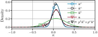
FIG. 15: One-dimensional density $\mathfrak{n}(\kappa)=p^{c}\mathfrak{n}^{c}+p^{t}\mathfrak{n}^{t}$ (133) ($p^{t}\!=\!0.51,p^{c}\!=\!0.49$) versus momentum detuning $\kappa$. The thermal cloud $\mathfrak{n}^{t}$ as well as the condensate $\mathfrak{n}^{c}$ obtained from (3+1)D GP simulation can be approximated with a Gaussian distribution $\mathfrak{n}^{a=\{c,t\}}\approx\tilde{\mathfrak{n}}^{a}$ (141).

Table 2: Experimental parameters: On the $J=\nicefrac{{1}}{{2}}\rightarrow J^{\prime}=\nicefrac{{3}}{{2}}$ transition, far-detuned, linearly polarized light couples only to one component of the dipole operator. Therefore, the transition strength is reduced by $\sqrt{3}$.

Quantity		Symbol		Value		Reference
Atom
Number of atoms in condensate		$N_{c}$		$(10\pm 1.)\text{\times}{10}^{3}$
Number of atoms in thermal cloud		$N_{t}$		$(7\pm 1.)\text{\times}{10}^{3}$
Atomic mass		$M$		86.909 180 520(15) u		[96]
Transition frequency Rb-87 D2		$\omega_{0}$		$2\pi\times 384.230\,484\,468\,5(62)\,$\mathrm{THz}$$		[97]
Lifetime		$\tau$		$26.2348\pm 0.0077\text{\,}\mathrm{ns}$		[98]
Decay rate		$\Gamma$		$2\pi\times$6.0666\pm 0.0018\text{\,}\mathrm{MHz}$$
D2 ($5^{2}S_{\nicefrac{{1}}{{2}}}\rightarrow 5^{2}P_{\nicefrac{{3}}{{2}}}$) transition dipole matrix element		$\mathcal{D}$		$3.58424(52)\times 10^{-29}\,$\mathrm{C}\text{\,}\mathrm{m}$$		[98]
Rabi-frequency		$\Omega_{0}$		$\mathcal{E}_{0}\mathcal{D}/\hbar\sqrt{3}$
Scattering length		$a$		$98.96\,a_{0}$		[99]
Trap frequencies		$[\omega_{x},\omega_{y},\omega_{z}]$		$2\pi\times[46\pm 2,18\pm 1,31\pm 1]\,$\mathrm{Hz}$$
Thomas-Fermi radii inside trap		$[r_{x},r_{y},r_{z}]$		$[4.2,10.8,6.2]\,$\mathrm{\SIUnitSymbolMicro m}$$
Laser
Wavelength		$\lambda_{L}$		$780.024\,500\,015\text{\,}\mathrm{nm}$
Wavenumber		$k_{L}$		$8.056\text{\,}\mathrm{\SIUnitSymbolMicro}\mathrm{m}^{-1}$
Detuning to atomic resonance		$\Delta$		$97.875\text{\,}\mathrm{GHz}$
Beam waist		$w_{0}$		$1.386\text{\,}\mathrm{mm}$
Rayleigh length		$x_{R}$		$7.7\text{\,}\mathrm{m}$
Total interaction time		$\Delta t$		$(10^{2}...10^{3})$\mathrm{\SIUnitSymbolMicro s}$$
Gaussian pulse width (47)		$\tau_{G}$		$\Delta t/8$
Distance between laser origins		$\ell$		$0.1\,x_{R}$
Total laser power		$P$		$\mathcal{E}_{0}^{2}\epsilon_{0}\pi cw_{0}^{2}/4$
Laser amplitude		$\mathcal{E}_{0}$

References

- Kazantsev et al. [1990] A. P. Kazantsev, G. I. Surdutovich, and V. P. Yakovlev, Mechanical Action of Light on Atoms (World Scientific, Singapore, 1990).
- Berman [1997] P. R. Berman, Atom Interferometry (Academic Press, 1997).
- Cronin et al. [2009] A. D. Cronin, J. Schmiedmayer, and D. E. Pritchard, Rev. Mod. Phys. 81, 1051 (2009).
- Tino and Kasevich [2014] G. M. Tino and M. A. Kasevich, Atom Interferometry (Societ Italiana di Fisica and IOS Press, Amsterdam, 2014).
- Abend et al. [2019] S. Abend, M. Gersemann, C. Schubert, et al., in Proc. Int. Sch. Phys. "Enrico Fermi", Vol. 197 (IOS Press, 2019) pp. 345–392, arXiv:2001.10976 .
- Fray et al. [2004] S. Fray, C. A. Diez, T. W. Hänsch, and M. Weitz, Phys. Rev. Lett. 93, 240404 (2004).
- Schlippert et al. [2014] D. Schlippert, J. Hartwig, H. Albers, et al., Phys. Rev. Lett. 112, 203002 (2014), arXiv:1406.4979 .
- Zhou et al. [2015] L. Zhou, S. Long, B. Tang, et al., Phys. Rev. Lett. 115, 013004 (2015), arXiv:1503.00401 .
- Altschul et al. [2015] B. Altschul, Q. G. Bailey, L. Blanchet, et al., Adv. Sp. Res. 55, 501 (2015), arXiv:1404.4307 .
- Bonnin et al. [2015] A. Bonnin, N. Zahzam, Y. Bidel, and A. Bresson, Phys. Rev. A 92, 023626 (2015), arXiv:1506.06535 .
- Barrett et al. [2016] B. Barrett, L. Antoni-Micollier, L. Chichet, et al., Nat. Commun. 7, 13786 (2016), arXiv:1609.03598 .
- Williams et al. [2016] J. Williams, S.-w. Chiow, N. Yu, and H. Müller, New J. Phys. 18, 025018 (2016), arXiv:1510.07780 .
- Asenbaum et al. [2020] P. Asenbaum, C. Overstreet, M. Kim, J. Curti, and M. A. Kasevich, Phys. Rev. Lett. 125, 191101 (2020), arXiv:2005.11624 .
- Arvanitaki et al. [2008] A. Arvanitaki, S. Dimopoulos, A. A. Geraci, J. Hogan, and M. Kasevich, Phys. Rev. Lett. 100, 120407 (2008).
- Bouchendira et al. [2011] R. Bouchendira, P. Cladé, S. Guellati-Khélifa, F. Nez, and F. Biraben, Phys. Rev. Lett. 106, 080801 (2011).
- Parker et al. [2018] R. H. Parker, C. Yu, W. Zhong, B. Estey, and H. Müller, Science 360, 191 (2018).
- Peters et al. [2001] A. Peters, K. Y. Chung, and S. Chu, Metrologia 38, 25 (2001).
- Mc Guirk et al. [2002] J. M. Mc Guirk, G. T. Foster, J. B. Fixler, M. J. Snadden, and M. A. Kasevich, Phys. Rev. A 65, 033608 (2002).
- Dimopoulos et al. [2007] S. Dimopoulos, P. W. Graham, J. M. Hogan, and M. A. Kasevich, Phys. Rev. Lett. 98, 111102 (2007).
- Aguilera et al. [2014] D. Aguilera, H. Ahlers, B. Battelier, et al., Class. Quantum Grav. 31, 115010 (2014).
- Dutta et al. [2016] I. Dutta, D. Savoie, B. Fang, et al., Phys. Rev. Lett. 116, 183003 (2016).
- Schkolnik et al. [2015] V. Schkolnik, B. Leykauf, M. Hauth, C. Freier, and A. Peters, Appl. Phys. B Lasers Opt. 120, 311 (2015), arXiv:1411.7914 .
- Xu et al. [2019] V. Xu, M. Jaffe, C. D. Panda, et al., Science 366, 745 (2019), arXiv:1907.03054 .
- Geiger et al. [2011] R. Geiger, V. Ménoret, G. Stern, et al., Nat. Commun. 2, 474 (2011), arXiv:1109.5905 .
- Müntinga et al. [2013] H. Müntinga, H. Ahlers, M. Krutzik, et al., Phys. Rev. Lett. 110, 093602 (2013), arXiv:1301.5883 .
- Kovachy et al. [2015a] T. Kovachy, P. Asenbaum, C. Overstreet, et al., Nature 528, 530 (2015a).
- Schuldt et al. [2015] T. Schuldt, C. Schubert, M. Krutzik, et al., Exp. Astron. 39, 167 (2015), arXiv:1412.2713 .
- Becker et al. [2018] D. Becker, M. D. Lachmann, S. T. Seidel, et al., Nature 562, 391 (2018), arXiv:1806.06679 .
- Elliott et al. [2018] E. R. Elliott, M. C. Krutzik, J. R. Williams, R. J. Thompson, and D. C. Aveline, npj Microgravity 4, 16 (2018).
- Tino et al. [2019] G. M. Tino, A. Bassi, G. Bianco, et al., Eur. Phys. J. D 73, 228 (2019), arXiv:1907.03867 .
- Chiow et al. [2011] S. W. Chiow, T. Kovachy, H. C. Chien, and M. A. Kasevich, Phys. Rev. Lett. 107, 130403 (2011).
- McDonald et al. [2013] G. D. McDonald, C. C. Kuhn, S. Bennetts, et al., Phys. Rev. A 88, 053620 (2013).
- Plotkin-Swing et al. [2018] B. Plotkin-Swing, D. Gochnauer, K. E. McAlpine, et al., Phys. Rev. Lett. 121, 133201 (2018), arXiv:1712.06738 .
- Gebbe et al. [2019] M. Gebbe, S. Abend, J.-N. Siemß, et al., “Twin-lattice atom interferometry,” (2019), arXiv:1907.08416 .
- Martin et al. [1988] P. J. Martin, B. G. Oldaker, A. H. Miklich, and D. E. Pritchard, Phys. Rev. Lett. 60, 515 (1988).
- Giltner et al. [1995] D. M. Giltner, R. W. McGowan, and S. A. Lee, Phys. Rev. Lett. 75, 2638 (1995).
- Oberthaler et al. [1996] M. K. Oberthaler, R. Abfalterer, S. Bernet, J. Schmiedmayer, and A. Zeilinger, Phys. Rev. Lett. 77, 4980 (1996).
- Kunze et al. [1996] S. Kunze, S. Dürr, and G. Rempe-Phd, Eur. Lett 34, 343 (1996).
- Giese et al. [2013] E. Giese, A. Roura, G. Tackmann, E. M. Rasel, and W. P. Schleich, Phys. Rev. A 88, 053608 (2013), arXiv:1308.5205 .
- Hartmann et al. [2020a] S. Hartmann, J. Jenewein, S. Abend, A. Roura, and E. Giese, Phys. Rev. A 102, 63326 (2020a), arXiv:2007.02635 .
- Kasevich and Chu [1991] M. Kasevich and S. Chu, Phys. Rev. Lett. 67, 181 (1991).
- Kasevich et al. [1991] M. Kasevich, D. S. Weiss, E. Riis, et al., Phys. Rev. Lett. 66, 2297 (1991).
- Neumann et al. [2020] A. Neumann, R. Walser, and W. Nörtershäuser, Phys. Rev. A 101, 052512 (2020).
- Hartmann et al. [2020b] S. Hartmann, J. Jenewein, E. Giese, et al., Phys. Rev. A 101, 53610 (2020b), arXiv:1911.12169 .
- Dahan et al. [1996] M. B. Dahan, E. Peik, J. Reichel, Y. Castin, and C. Salomon, Phys. Rev. Lett. 76, 4508 (1996).
- Wilkinson et al. [1996] S. R. Wilkinson, C. F. Bharucha, K. W. Madison, Q. Niu, and M. G. Raizen, Phys. Rev. Lett. 76, 4512 (1996).
- Peik et al. [1997] E. Peik, M. Ben Dahan, I. Bouchoule, Y. Castin, and C. Salomon, Phys. Rev. A 55, 2989 (1997).
- Müller et al. [2009] H. Müller, S.-w. Chiow, S. Herrmann, and S. Chu, Phys. Rev. Lett. 102, 240403 (2009), arXiv:0903.4192 .
- Cladé et al. [2009] P. Cladé, S. Guellati-Khélifa, F. Nez, and F. Biraben, Phys. Rev. Lett. 102, 240402 (2009).
- McAlpine et al. [2020] K. E. McAlpine, D. Gochnauer, and S. Gupta, Phys. Rev. A 101, 023614 (2020), arXiv:1912.08902 .
- Müller et al. [2008a] H. Müller, S.-w. Chiow, and S. Chu, Phys. Rev. A 77, 023609 (2008a).
- Kovachy et al. [2012] T. Kovachy, S. W. Chiow, and M. A. Kasevich, Phys. Rev. A 86, 011606(R) (2012).
- Kovachy et al. [2015b] T. Kovachy, P. Asenbaum, C. Overstreet, et al., Nature 528, 530 (2015b).
- Ahlers et al. [2016] H. Ahlers, H. Müntinga, A. Wenzlawski, et al., Phys. Rev. Lett. 116, 173601 (2016).
- Szigeti et al. [2012] S. S. Szigeti, J. E. Debs, J. J. Hope, N. P. Robins, and J. D. Close, New J. Phys. 14, 023009 (2012).
- Gochnauer et al. [2019] D. Gochnauer, K. E. McAlpine, B. Plotkin-Swing, A. O. Jamison, and S. Gupta, Phys. Rev. A 100, 043611 (2019), arXiv:1906.09328 .
- Siemß et al. [2020] J.-N. Siemß, F. Fitzek, S. Abend, et al., Phys. Rev. A 102, 033709 (2020), arXiv:2002.04588v1 .
- Müller et al. [2008b] H. Müller, S.-W. Chiow, Q. Long, S. Herrmann, and S. Chu, Phys. Rev. A 100, 180405 (2008b).
- Bernhardt and Shore [1981] A. F. Bernhardt and B. W. Shore, Phys. Rev. A 23, 1290 (1981).
- Sulzbach et al. [2019] R. Sulzbach, T. Peters, and R. Walser, Phys. Rev. A 100, 013847 (2019).
- Yoshida [1990] H. Yoshida, Phys. Lett. A 150, 262 (1990).
- Puri [2001] R. R. Puri, Mathematical Methods of Quantum Optics, Springer Series in Optical Sciences (Springer, Berlin, Heidelberg, 2001).
- McCall and Hahn [1970] S. L. McCall and E. L. Hahn, Phys. Rev. A 2, 861 (1970).
- Allen and Eberly [1987] L. Allen and J. H. Eberly, Optical Resonance and Two-level Atoms (Dover, New York, 1987).
- Sturm et al. [2014] M. R. Sturm, B. Rein, T. Walther, and R. Walser, J. Opt. Soc. Am. B 31, 1964 (2014).
- Brion et al. [2007] E. Brion, L. H. Pedersen, and K. Mølmer, J. Phys. A Math. Theor. J. 40, 1033 (2007).
- Marksteiner et al. [1995] S. Marksteiner, R. Walser, P. Marte, and P. Zoller, Appl. Phys. B Laser Opt. 60, 145 (1995).
- Olver et al. [2010] F. W. Olver, D. W. Lozier, F. Boisvert, Ronald, and C. W. Clark, NIST Handbook of Mathematical Functions (National Institute of Standards and Technology and Cambridge University Press, 2010).
- Wilkens et al. [1991] M. Wilkens, E. Schumacher, and P. Meystre, Phys. Rev. A 44, 3130 (1991).
- Champenois et al. [2001] C. Champenois, M. Büchner, R. Delhuille, et al., Eur. Phys. J. D 13, 271 (2001).
- Kohn [1959] W. Kohn, Phys. Rev. 115, 809 (1959).
- Callaway [1991] J. Callaway, Quantum Theory of the Solid State (Academic Press, New York, 1991).
- Grupp et al. [2007] M. Grupp, R. Walser, W. P. Schleich, A. Muramatsu, and M. Weitz, J. Phys. B At. Mol. Opt. Phys. 40, 2703 (2007).
- Sturm et al. [2017] M. R. Sturm, M. Schlosser, R. Walser, and G. Birkl, Phys. Rev. A 95, 063625 (2017), arXiv:1705.01271 .
- Demkov and Kunike [1969] Y. N. Demkov and M. Kunike, Vestn. Leningr. Univ. Fiz. Khim 16, 39 (1969).
- Vitanov [2007] N. V. Vitanov, New J. Phys. 9, 58 (2007).
- Ewald [1917] P. P. Ewald, Ann. Phys. 24, 557 (1917).
- Zeilinger [1986] A. Zeilinger, Phys. B+C 137, 235 (1986).
- Kato [1949] T. Kato, Prog. Theor. Phys. 4, 514 (1949).
- Beckett [1956] S. Beckett, Waiting for Godot (Faber and Faber, London, 1956).
- [81] A. Neumann, Aberrations of atomic diffraction - From ultracold atoms to hot ions, Doctoral dissertation, University of Darmstadt.
- Tong et al. [2007] D. M. Tong, K. Singh, L. C. Kwek, and C. H. Oh, Phys. Rev. Lett. 98, 150402 (2007).
- Siegman [1986] A. E. Siegman, Lasers (University Science Books, 1986).
- van Zoest et al. [2010] T. van Zoest, N. Gaaloul, Y. Singh, et al., Science 328, 1540 (2010).
- Ketterle et al. [1999] W. Ketterle, D. S. Durfee, and D. M. Stamper-Kurn, Making, probing and understanding Bose-Einstein condensates, Tech. Rep. (1999) arXiv:9904034 [cond-mat] .
- Gottfried and Yan [2003] K. Gottfried and T.-M. Yan, Quantum Mechanics: Fundamentals, 2nd ed. (Springer, New York, 2003).
- Teske et al. [2018] J. Teske, M. R. Besbes, B. Okhrimenko, and R. Walser, Phys. Scr. 93, 124004 (2018).
- Akhiezer and Peletminskii [1981] A. I. Akhiezer and S. V. Peletminskii, Methods of Statistical Physics (Pergamon Press Ltd., Oxford, 1981).
- Proukakis et al. [2013] N. Proukakis, S. Gardiner, M. Davis, and M. Szymańska, Quantum Gases: Finite Temperature and Non-Equilibrium Dynamics, Cold Atoms, Vol. 1 (Imperial College Press, London, 2013).
- Walser et al. [2000] R. Walser, J. Cooper, and M. Holland, Phys. Rev. A 63, 013607 (2000).
- Damon et al. [2014] F. Damon, F. Vermersch, J. G. Muga, and D. Guéry-Odelin, Phys. Rev. A 89, 053626 (2014).
- Castin and Dum [1996] Y. Castin and R. Dum, Phys. Rev. Lett. 77, 5315 (1996), arXiv:9604005 [quant-ph] .
- Kagan et al. [1996] Y. Kagan, E. L. Surkov, and G. V. Shlyapnikov, Phys. Rev. A 54, R1753 (1996).
- Kagan et al. [1997] Y. Kagan, E. L. Surkov, and G. V. Shlyapnikov, Phys. Rev. A 55, R18 (1997).
- Meister et al. [2017] M. Meister, S. Arnold, D. Moll, et al., in Adv. At. Mol. Opt. Phys., Vol. 66 (Academic Press Inc., 2017) pp. 375–438, arXiv:1701.06789 .
- Bradley et al. [1999] M. P. Bradley, J. V. Porto, S. Rainville, J. K. Thompson, and D. E. Pritchard, Phys. Rev. Lett. 83, 4510 (1999).
- Ye et al. [1996] J. Ye, S. Swartz, P. Jungner, and J. L. Hall, Opt. Lett. 21, 1280 (1996).
- Steck [2019] D. A. Steck, “Rubidium 87 D Line Data (revision 2.2.1),” (2019).
- Marte et al. [2002] A. Marte, T. Volz, J. Schuster, et al., Phys. Rev. Lett. 89, 283202 (2002).