Quasinormal modes and Purcell factors of coupled loss-gain resonators and index-modulated ring resonators near exceptional points

Abstract

We first present a quasinormal mode (QNM) theory for coupled loss and gain resonators, working in the vicinity of an exceptional point. Assuming linear media, which can be fully quantified using the complex pole properties of the QNMs, we show how the QNMs yield a quantitatively good model to a full dipole spontaneous emission response in Maxwell’s equations at a variety of spatial positions and frequencies (linear response). We also develop a highly accurate and intuitive QNM coupled-mode theory, which can be used to rigorously model such systems using only the QNMs of the bare resonators, where the hybrid QNMs of the complete system are automatically obtained. Near a lossy exceptional point, we analytically show how the QNMs yield a Lorentzian-like and a Lorentzian-squared-like response for the spontaneous emission lineshape, consistent with other works. However, using rigorous analytical and numerical solutions for microdisk resonators, we demonstrate that the general lineshapes are far richer than what has been previously predicted. Indeed, the classical picture of spontaneous emission can take on a wide range of positive and negative Purcell factors from the hybrid modes of the coupled loss-gain system. These negative Purcell factors are unphysical and signal a clear breakdown of the classical dipole picture of spontaneous emission in such media, though the negative local density of states is correct. We also show the rich spectral features of the Green function propagators, which can be used to model various physical observables. Second, we present a QNM approach to model index-modulated ring resonators working near an exceptional point and show unusual chiral power flow from linearly polarized emitters, in agreement with recent experiments, which is quantitatively explained without invoking the interpretation of a missing dimension (the Jordan vector) and a decoupling from the cavity eigenmodes.

I Introduction

Lossless photonic systems (such as closed resonators with no material absorption) can be formulated as a Hermitian eigenvalue problem, which yields real eigenfrequencies from the source-free Helmholz equation, and corresponding normal modes (NMs). This is also true for periodic systems with bound modes, e.g., lossless waveguide modes. However, real cavity structures (resonators) with open boundary conditions yield finite loss (or gain) and produce complex eigenfrequencies. Thus most optical systems are naturally dissipative via material absorption and/or radiation.

A common design approach to improving resonators is to increase the photonic local density of states (LDOS), by reducing radiation losses and the effective mode volume, thus increasing the Purcell factor for enhanced spontaneous emission (SE). An alternative approach to reducing loss is through gain compensation, where a gain medium can be introduced and controlled through stimulated emission or parametric processes. Not necessarily related to lasing, a gain medium can be introduced to the system and treated as a linear amplifying medium Raabe and Welsch (2008); Søndergaard and Tromborg (2001), which must satisfy strict criteria that relates to the complex poles of the Green function. Aided by the rapid development of optical nanotechnologies, coupled loss and gain structures have been under intense investigation recently, especially after the demonstrations of parity-time (PT) symmetry Bender and Boettcher (1998); Bender et al. (1999); Lévai and Znojil (2000); Bender et al. (2002a, b); Mostafazadeh (2002); Bender et al. (2003); Bender (2007) in optical systems El-Ganainy et al. (2007); Makris et al. (2008); Klaiman et al. (2008); Guo et al. (2009); Longhi (2009); Mostafazadeh (2009); Rüter et al. (2010); Kottos (2010); Longhi (2010a); Benisty et al. (2015); Konotop et al. (2016); Feng et al. (2017); Longhi (2017); Lupu et al. (2017); El-Ganainy et al. (2018); Jin (2018); Morozko et al. (2020), which support so-called exceptional points (EPs) Berry (2004); Heiss (2004, 2012); Ding et al. (2016); Miri and Alù (2019); Chen et al. (2019); Jin et al. (2020) (two isolated eigenfrequencies and eigenmodes coalesce), along with many interesting and counter-intuitive phenomena, such as non-reciprocal propagation (isolators) Lin et al. (2011); Feng et al. (2013); Peng et al. (2014a); Chang et al. (2014); Jin and Song (2018), mode switching Zyablovsky et al. (2014); Doppler et al. (2016); Xu et al. (2016); Heiss (2016), efficient sensing Chen et al. (2017, 2018), absorber Longhi (2010b); Chong et al. (2011); Sun et al. (2014); Jin et al. (2016), and lasing Brandstetter et al. (2014); Feng et al. (2014); Hodaei et al. (2014); Peng et al. (2014b).

To have a detailed understanding of such systems, and also for connecting to new applications in quantum optics, it is desirable to have an accurate model of coupled loss-gain resonators at the level of a rigorous and intuitive mode theory, which can allow one to describe light-matter interactions at various spatial points and frequencies. From a theoretical perspective, temporal coupled mode theory (CMT) has proved to be an efficient approach to investigate coupled resonator systems Haus and Huang (1991); Fan et al. (2003), where only the solution from the bare systems are required, and one assumes that the coupled modes can be represented by a linear superposition of the bare modes (weak coupling regime). However, the coupling coefficients are typically used as heuristic parameters in that they are usually extracted from fitting the full solution of the coupled system properties Artar et al. (2011); Peng et al. (2014a); Yang et al. (2019); Park et al. (2020), or they are mainly used to explain the basic physics of coupling.

Another potential problem with such approaches is that the underlying modes of the bare resonators are assumed to be NMs (Hermitian system), and a finite decay rate, to account for real losses, is added phenomenologically. This finite decay rate already relates to a non-Hermitian problem, so it is natural to model the bare resonators also with a non-Hermitian theory, where the correct eigenvalues and modes would then be obtained for a more general CMT for loss-gain systems. This is not only a more correct approach, but it changes some of the fundamental coupling regimes and constraints significantly, and open up much richer light-matter interaction regimes.

In recent years, the theory of open cavity modes has been shown to be accurately described in terms of quasinormal modes (QNMs) Lai et al. (1990); Leung et al. (1994a, b); Leung and Pang (1996); Lee et al. (1999); Kristensen et al. (2012); Sauvan et al. (2013); Kristensen and Hughes (2014); Bai et al. (2013); Zschiedrich et al. (2018); Alpeggiani et al. (2017); Lalanne et al. (2018); Kristensen et al. (2020), which are open cavity modes with complex eigenfrequencies and spatially diverging modes (with finite loss). These open cavity modes naturally include the effect of losses and can also be used to construct the photon Green function, which describes a wide range of light-matter interactions Lee et al. (1999); Muljarov et al. (2010); Kristensen et al. (2012); Sauvan et al. (2013); Kristensen and Hughes (2014); Muljarov and Langbein (2016); Lalanne et al. (2018); Kristensen et al. (2020). Moreover, as shown recently, QNMs can be fully quantized and used to show departures from the usual NM quantum optics theories Franke et al. (2019, 2020a, 2020b). Several CMT approaches based on QNMs have also been successfully developed Vial and Hao (2016); Kristensen et al. (2017); Cognée (2020); Tao et al. (2020) for coupled passive resonator systems.

In this work, we first present a QNM theory for general media containing both lossy resonators and gain resonators. We describe a rigorous and intuitive CMT based on the Green function solution for the coupled loss-gain QNMs, where we analytically obtain the hybrid modes from only the QNMs of the bare resonators (gain or loss). We demonstrate the extremely high accuracy of the analytical theory by comparing with full numerical dipole simulations for whispering-gallery modes (WGMs) of microdisk resonators, and show excellent agreement for various designs and spatial positions without using any fitting parameters. A QNM approach also allows one to justify the the underlying assumptions of a linear gain medium, which requires an analysis of the complex poles. Without such an analysis, then composite systems may not even constitute a physically meaningful solution with gain treated at the level of a material response in Maxwell’s equations. Indeed, as far as we are aware, this is likely the only approach to confirm this directly (in the absence of having an analytical expression for the medium Green function).

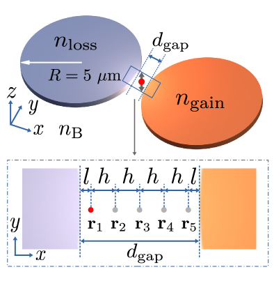
Figure 1: Schematic diagram of a coupled loss and gain microdisk resonator system. The radius of both resonators is $R=5\,\mu$m. The refractive index of the lossy (gain) resonator is $n_{\rm loss}$ ($n_{\rm gain}$), in a background medium with $n_{\rm B}=1$ (free space). The gap distance between the resonators is $d_{\rm gap}$, and the dipole (emitter) is placed within the gap, at several possible positions: $\mathbf{r}_{1}$, $\mathbf{r}_{2}$, $\mathbf{r}_{3}$, $\mathbf{r}_{4}$, and $\mathbf{r}_{5}$ (see text). The origin of the coordinate system is at the gap center.

After obtaining the physically meaningful QNMs for loss-gain resonator systems, we apply our theory to study the unusual Purcell factors and Green function propagators at various spatial positions for eigenfrequencies close to an EP. For our numerical example, the considered coupled loss-gain disk resonators are shown in Fig. 1(a), where one microdisk has material loss and the other has material gain. Such systems with balanced gain and loss form a general optical system to investigate PT symmetry and EP physics Chang et al. (2014); Peng et al. (2014a); Chen et al. (2018). In our model, we choose a gain coefficient that is slightly less than the loss coefficient, which can support hybridized QNMs with finite loss, which is also a requirement for assuming linear gain media Raabe and Welsch (2008).

Next, we apply our general QNM approach to model emitters coupled to index-modulated ring resonators, which were recently experimentally studied Chen et al. (2020); in this work, the authors found the following interesting observation, quoting from their abstract: “We find a chirality-reversal phenomenon in a ring cavity where the radiation field reveals the missing dimension of the Hilbert space, known as the Jordan vector. This phenomenon demonstrates that the radiation field of an emitter can become fully decoupled from the eigenstates of its environment.” In contrast to this interpretation, using similar resonator designs, we show that the chiral reversal behaviour is quantitatively explained by the emitter coupling to the two fundamental QNMs of the resonator structure. We explain this net chiral power flow analytically in terms of only the QNM properties, and show excellent agreement with full dipole simulations from Maxwell’s equations.

The rest of our paper is organized as follows: In Sec. II, we introduce optical QNMs, Green functions in terms of QNMs, and show how these relate to SE decay and Purcell factors. In Sec. III, we present a detailed CMT, using both NMs and QNMs, to obtain analytical insight into coupled loss-gain resonators. We subsequently use these to explain when an EP may form, and how things change when one uses a QNM theory. We obtain explicit expressions for the hybrid modes using only the QNMs of the bare loss or gain resonators. We explain the limits and failures of the usual CMT for such systems. Section IV discusses Green functions and Purcell factors at the EP, and shows how a Lorentzian-like or Lorentzian-squared-like lineshape forms Yoo et al. (2011); Pick et al. (2017a); Khanbekyan and Wiersig (2020). Section V presents detailed numerical results for coupled microdisk resonators, and confirms the excellent agreement with our analytical CMT and full dipole solutions, for various gap distances between the resonators. We then study various Purcell factor regimes at different dipole positions as a function of frequency, and show highly unusual and rich spectral lineshapes, including negative Purcell factors, and discuss the essential role of the QNM phase; again, all of these show quantitatively good agreement with full dipole calculations. Negative total purcell factors are not physical and motivate the need for a corrected derivation of the accepted Fermi’s golden rule for such media, which is described elsewhere Franke et al. (2021). We also show the Green function propagators, which connects to various observables outside the resonators, which also yield rich non-Lorentzian lineshapes. Finally, in Sec. VI, we study EP physics for emitters coupled to index-modulated ring resonators, and connect to recent experiments on chiral emission for linear dipoles Chen et al. (2020) using the QNM theory. We give our conclusions in Sec. VII.

In addition to the main text, we also present several Appendices. Appendix A discusses the numerical QNM normalization approaches using COMSOL, where we show three different approaches yielding the same normalized QNMs within numerical precision. Appendix LABEL:sec:degenerate_WGMs discusses why we only need to consider one QNM of the miscrodisk resonator for the dipole locations we study, which is constructed from a symmetric linear combination of clockwise and counter clockwise WGMs. Full dipole calculations in COMSOL are also discussed in Appendix LABEL:sec:full_simulation, which are used to check the validity of the QNM results. To compare with the coupled cavity systems, the results for single loss and single gain cavities are shown in Appendix LABEL:sec:single_modes, which also confirms the extremely high accuracy of the single QNM approximation for these resonators. Naturally, one can also solve the coupled system with a QNM approach directly, instead of using CMT from the bare solutions; thus Appendix LABEL:sec:directQNMs shows the direct QNM approach for a coupled resonators, where quantitatively good agreement with our analytical CMT results and full dipole results are obtained. In addition to the loss-gain cavities shown in the main text, we also show two more loss-gain examples in Appendix F, with different gain coefficients.

II Quasinormal modes and semiclassical theory of spontaneous emission and Purcell factors

We first introduce the electric-field QNMs, $\tilde{\mathbf{f}}_{{\mu}}\left(\mathbf{r}\right)$, which are solutions to the Helmholtz equation,

$$\bm{\nabla}\times\bm{\nabla}\times\tilde{\mathbf{f}}_{{\mu}}\left(\mathbf{r}\right)-\left(\dfrac{\tilde{\omega}_{{\mu}}}{c}\right)^{2}\epsilon(\mathbf{r},\tilde{\omega}_{\mu})\,\tilde{\mathbf{f}}_{{\mu}}\left(\mathbf{r}\right)=0,$$ (1)

where $c$ is the vacuum speed of light, $\tilde{\omega}_{{\mu}}=\omega_{{\mu}}-i\gamma_{{\mu}}$ is the complex eigenfrequency of each QNM, and $\epsilon(\mathbf{r},\tilde{\omega}_{\mu})$ is the dielectric function, which is in general complex and dispersive, though for our numerical examples below, we will assume this is a constant complex value in the frequency regime of interest (this is not a model restriction). The open boundary conditions ensure the Silver-Müller radiation condition Kristensen et al. (2015). It is also worth noting that this boundary condition leads to quite different asymptotic behaviour of gain QNMs and loss QNMs due to the change of sign for $\gamma_{\mu}$. Namely, the lossy QNMs diverge in space but converge in time, while the gain QNMs converge in space, but diverge in time. For the composite system, then the hybrid modes must converge in time, forcing the complex poles to have loss. These subtleties are clearly missing and overlooked in heuristic theories of coupled loss and gain resonators, but are essential to get correct for a physically meaningful model.

Using $n$ to represent the refractive index and $\alpha$ the loss or gain coefficient, for a lossy resonator with permittivity $\epsilon_{\rm L}=(n_{\rm L}+i\alpha_{\rm L})^{2}$, we assume a dominant QNM resonance $\tilde{\omega}_{\rm L}\approx\omega_{\rm L}-i\gamma_{\rm L}$, where $\alpha_{\rm L},\gamma_{\rm L}>0$. Similarly, for the gain resonator, $\epsilon_{\rm G}=(n_{\rm G}+i\alpha_{\rm G})^{2}$, we have a dominant QNM resonance $\tilde{\omega}_{\rm G}\approx\omega_{\rm L}-i\gamma_{\rm G}$, where now $\alpha_{\rm G},\gamma_{\rm G}<0$. The quality factor is defined from $Q_{\mu}=\omega_{\mu}/(2|\gamma_{\mu}|)$. Since we treat the gain amplifier in terms of a linear amplifying medium (e.g., we neglect saturation effects in the gain medium), the composite system must have $\gamma_{\mu}^{+/-}{>}0$ for the hybrid modes Raabe and Welsch (2008). We will refer to the gain and loss QNMs as $\tilde{\bf f}^{\rm G}$ and $\tilde{\bf f}^{\rm L}$, respectively, and the hybrid modes (i.e., in the presence of coupling) as $\tilde{\bf f}^{\pm}$.

To connect to a general definition of the SE in an arbitrary medium, we seek to obtain the Green function, defined through

$$\bm{\nabla}\times\bm{\nabla}\times{{\bf G}}({\bf r},{\bf r}_{0},\omega)-\frac{\omega^{2}}{c^{2}}\epsilon({\bf r},\omega){{\bf G}}({\bf r},{\bf r}_{0},\omega)=\frac{\omega^{2}}{c^{2}}{\bf 1}\delta({\bf r}-{\bf r}_{0}),$$ (2)

with corresponding radiation conditions, and $\mathbf{1}$ is the unit tensor. The normalized QNMs can be used to define the Green function for locations near (or within) the scattering geometry through Leung et al. (1994a); Ge et al. (2014)

$$\mathbf{G}\left(\mathbf{r},\mathbf{r}_{0},\omega\right)=\sum_{\mu}A_{\mu}\left(\omega\right)\,\tilde{\mathbf{f}}_{\mu}\left({\bf r}\right)\tilde{\mathbf{f}}_{\mu}\left({\bf r}_{0}\right),$$ (3)

with $A_{\mu}(\omega)={\omega}/{2(\tilde{\omega}_{\mu}-\omega)}$. Expanding the Green function with the QNMs can easily be used to compute the SE rate and the Purcell factor. We stress again that the medium must meet the condition for linear amplifying media, which coincides with a causal Green function in the sense of linear response theory (Kramers-Krönig relations). Here, the Green function must be analytic in the upper half complex plane to fulfill the Kramers-Krönig relations, and this can be rigorously justified by using a QNM approach. Indeed, without such an approach, it is not known whether the model represents a physically meaningful solution for Maxwell’s equations.

Considering a dipole emitter, $\mathbf{d}=d_{0}\mathbf{n}_{\rm d}$, at location ${\bf r}_{\rm d}$, then the classical SE rate is  Kristensen and Hughes (2014)

$$\begin{split}\Gamma(\mathbf{r}_{\rm d},\omega)&=\frac{2}{\hbar\epsilon_{0}}\mathbf{d}\cdot{\rm Im}\{\mathbf{G}(\mathbf{r}_{\rm d},\mathbf{r}_{\rm d},\omega)\}\cdot\mathbf{d},\end{split}$$ (4)

and the generalized Purcell factor reads Anger et al. (2006); Kristensen and Hughes (2014)

$$\begin{split}&F(\mathbf{r}_{\rm d},\omega)=1+\frac{\Gamma(\mathbf{r}_{\rm d},\omega)}{\Gamma_{0}(\mathbf{r}_{\rm d},\omega)},\end{split}$$ (5)

where $\Gamma_{0}(\mathbf{r}_{\rm d},\omega)=2\mathbf{d}\cdot{\rm Im}\{\mathbf{G}_{\rm B}(\mathbf{r}_{\rm d},\mathbf{r}_{\rm d},\omega)\}\cdot\mathbf{d}/(\hbar\epsilon_{0})$, and ${\bf G}_{\rm B}$ is the Green function for a homogeneous medium (known analytically). For a 2D TM (TE) dipole, ${\rm Im}\{\mathbf{G}_{\rm B}(\mathbf{r}_{\rm d},\mathbf{r}_{\rm d},\omega)\}={\omega^{2}}/{4c^{2}}$ (${\omega^{2}}/{8c^{2}}$). The factor of 1 appears naturally for dipole positions outside the resonator Ge and Hughes (2014).

For an arbitrary photonic cavity medium, the QNMs for both the bare resonators (i.e., without coupling), and also for the coupled system, can be obtained from an efficient dipole scattering approach in complex frequency Bai et al. (2013), described in more detail in Appendix A. The total Green function can also be obtained numerically from the full dipole response (i.e., without any modal approximations), which we carry out in COMSOL to check the accuracy of the QNM expansion form. Although the hybrid QNMs can be obtained numerically as well, it is far more insightful to develop a coupled-mode formalism to describe the coupling geometry.

III Coupled Mode Theory with an intuitive Green function expansion

III.1 Wave equation and normal modes

Before developing a QNM CMT, here we present a NM approach and also connect to the common literature for describing when EPs can occur for coupled loss-gain cavity modes.

To simplify the equations and terminology, we introduce shorthand notation, and define the wave equation:

$${\cal L}\ket{\bf E}=\omega^{2}\hat{\epsilon}_{\rm t}\ket{\bf E},$$ (6)

where the fields are assumed to have a harmonic frequency dependence, $e^{-i\omega t}$, ${\cal L}=c^{2}\bm{\nabla}\times\bm{\nabla}\times$, and $\epsilon_{\rm t}({\bf r})$ is the total dielectric constant that we will assume is nondispersive. The operator $\hat{\epsilon}_{\rm t}$ is defined as $\braket{{\bf r}}{\hat{\epsilon}_{\rm t}}{{\bf r}^{\prime}}=\epsilon_{\rm t}({\bf r}){\bf\delta}({\bf r}-{\bf r}^{\prime})$, and the electric field is given by a projection onto space, $\braket{{\bf r}}{{\bf E}}={\bf E}({\bf r},\omega)$.

To construct a Green function solution, we consider a situation where we start with cavity 1, and then add cavity 2. The dielectric constant defining cavity 1 is $\hat{\epsilon}_{1}=\hat{\epsilon}_{\rm b}+\hat{V}_{1}$, so we can also write the wave equation as

$$({\cal L}-\omega^{2}\hat{\epsilon}_{1})\ket{\bf E}=\omega^{2}\hat{V}_{2}\ket{\bf E},$$ (7)

where $\hat{V}_{2}$ defines the dielectric constant change after adding in cavity 2, and $\hat{\epsilon}_{\rm b}$ defines the entire background without either cavity. Naturally, we can also start from cavity 2 and add in cavity 1, and the end Green function that includes both cavities must be the same.

III.2 Coupled mode theory and lossless exceptional points using normal modes

Exploiting the fact that ${\cal L}$ is a linear self-adjoint operator over space, the homogeneous part of Eq. (7) defines an orthogonal set of eigenstates on a single cavity. It follows that

$${\cal L}\ket{{\bf f}_{k}}=\omega_{k}^{2}\hat{\epsilon}_{1}\ket{{\bf f}_{k}},$$ (8)

where $\omega_{k}$ are the eignfrequencies of the eigenstates ${\bf f}_{k}$. These states are also complete and orthogonal Cowan and Young (2003), so

$$\sum_{k}\hat{\epsilon}_{1}\ket{{\bf f}_{k}}\bra{{\bf f}_{k}} ={\bf 1},$$

$$\braket{{\bf f}_{i}}{\hat{\epsilon}_{1}}{{\bf f}_{j}} =\delta_{ij},$$ (9)

and the sum includes all modes, physical and unphysical.

Next, we can formulate a scattering problem, based on some (arbitrary) reference input field, so that

$$\ket{\bf E}=\ket{{\bf E}^{\rm 0}}+\hat{\bf G}\hat{V}_{2}\ket{{\bf E}^{0}},$$ (10)

where ${\bf G}({\bf r},{\bf r}^{\prime})=\braket{{\bf r}}{\hat{\bf G}}{{\bf r}^{\prime}}$ is the total Green function of the system (including both cavities), and is defined from

$$({\cal L}-\omega^{2}\hat{\epsilon}_{1}-\omega^{2}\hat{V}_{2})\hat{\bf G}=({\cal L}-\omega^{2}\hat{\epsilon}_{\rm t})\hat{\bf G}=\omega^{2}{\bf 1}.$$ (11)

For weakly coupled resonators, we can expand $\hat{\bf G}$ in terms of a restricted set of carefully chosen basis states, which will be the dominant modes of the individual cavity systems Cowan and Young (2003). Thus one obtains the Green function expansion

$$\hat{\bf G}=\sum_{\alpha,\beta}B_{\alpha,\beta}\ket{{\bf f}_{\alpha}}\bra{{\bf f}_{\beta}},$$ (12)

where both sums extend over all states of interest. If we obtain a solution for $B_{\alpha,\beta}$, then the scattering problem is solved as we have the total Green function, including the new poles of the coupled resonator system.

In the absence of cavity 2, we define the cavity mode of the bare cavity 1 (i.e., no cavity mode 2 yet), from

$${\cal L}\ket{{\bf f}_{1}}=\omega_{1}^{2}\hat{\epsilon}_{1}\ket{{\bf f}_{1}},$$ (13)

with the normalization $\braket{{\bf f}_{1}}{\hat{\epsilon}_{1}}{{\bf f}_{1}}=1$. For simplicity, we assume the cavity supports a dominant single mode in the frequency of interest, but this can easily be generalized to allow for $N$ modes per cavity. Similarly, we can define the solution of cavity 2, from

$${\cal L}\ket{{\bf f}_{2}}=\omega_{2}^{2}\hat{\epsilon}_{2}\ket{{\bf f}_{2}},$$ (14)

with $\braket{{\bf f}_{2}}{\hat{\epsilon}_{2}}{{\bf f}_{2}}=1$.

Subsequently, we substitute the mode expansions into the main Green function Eq. (11), to obtain

$$\sum_{\alpha,\beta}[\omega_{\alpha}^{2}\braket{{\bf f}_{i}}{\hat{\epsilon}_{\alpha}}{{\bf f}_{\alpha}} -\omega^{2}\braket{{\bf f}_{i}}{\hat{\epsilon}_{\rm t}}{{\bf f}_{\alpha}}]B_{\alpha,\beta}\braket{{\bf f}_{\beta}}{\hat{\epsilon}_{\rm t}}{{\bf f}_{j}}$$

$$=\omega^{2}\braket{{\bf f}_{i}}{\hat{\epsilon}_{\rm t}}{{\bf f}_{j}},$$ (15)

where $i,j$ refer to any basis states, and $\hat{\epsilon}_{\alpha}$ can refer to $\hat{\epsilon}_{1}$ or $\hat{\epsilon}_{2}$. Equation (III.2) defines a matrix equation whose poles correspond to the new eigenfrequencies of the composite system. To proceed, we exploit the fact that the modes are only weakly coupled to each other, and so

$$\braket{{\bf f}_{\alpha}}{\hat{\epsilon}_{\rm t}}{{\bf f}_{\beta}}=\delta_{\alpha\beta},$$ (16)

which can typically be easily checked numerically (else this approximation can also be relaxed, which just yields a more complex matrix to be solved).

The matrix defined from Eq. (III.2), namely $MBT=T$, has the solution $B_{\alpha,\beta}=[M^{-1}]_{\alpha,\beta}$, with elements:

$$M_{\alpha,\alpha} =\frac{1}{\omega^{2}}(\omega_{\alpha}^{2}-\omega^{2}),$$

$$M_{\alpha,\beta\neq\alpha} =\frac{1}{\omega^{2}}(-\omega_{\beta}^{2}\braket{\braket{{\bf f}_{\alpha}}{\hat{V}_{\alpha}}{{\bf f}_{\beta}}}{)}{.}$$ (17)

Thus, the matrix $M$ is

$$M=\frac{1}{\omega^{2}}\begin{pmatrix}\omega_{1}^{2}-\omega^{2}&-{\omega_{2}^{2}}\braket{{\bf f}_{1}}{\hat{V}_{1}}{{\bf f}_{2}}\\ -{\omega_{1}}^{2}\braket{{\bf f}_{2}}{\hat{V}_{2}}{{\bf f}_{1}}&\omega_{2}^{2}-\omega^{2}\end{pmatrix},$$ (18)

and we define the inter-mode coupling rate:

$$\kappa_{12}=\frac{\omega_{2}}{2}\braket{{\bf f}_{1}}{\hat{V}_{1}}{{\bf f}_{2}},$$ (19)

so that

$$M=\frac{1}{\omega^{2}}\begin{pmatrix}\omega_{1}^{2}-\omega^{2}&-2{\omega_{2}}\kappa_{12}\\ -2{\omega_{1}}\kappa_{21}&\omega_{2}^{2}-\omega^{2}\end{pmatrix}.$$ (20)

Matrix inversion can be solved without approximations, however it is appropriate to obtain an easier form within a rotating-wave approximation. Using $\omega_{\alpha}^{2}-\omega^{2}\approx(\omega_{\alpha}-\omega)2\omega_{\alpha}\approx(\omega_{\alpha}-\omega)2\omega$, then

$$M=\frac{2}{\omega}\begin{pmatrix}\omega_{1}-\omega&-\kappa_{12}\\ -\kappa_{21}&\omega_{2}-\omega\end{pmatrix},$$ (21)

and we obtain an explicit solution for the Green function expansion coefficients

$$B_{\alpha,\beta}=\frac{\omega/2}{(\omega-\omega_{+})(\omega-\omega_{-})}\begin{pmatrix}\omega_{2}-\omega&\kappa_{12}\\ \kappa_{21}&\omega_{1}-\omega\end{pmatrix},$$ (22)

where the pole frequencies are

$$\omega_{\pm}=\frac{\omega_{1}+\omega_{2}}{2}\pm\frac{\sqrt{4\kappa_{12}\kappa_{21}+(\omega_{1}-\omega_{2})^{2}}}{2}.$$ (23)

Finally, we note that for closed cavity systems, unitarity of a Hermitian system also requires that $\kappa_{12}=\kappa_{21}^{*}$, and the pole frequencies are simply

$$\omega_{\pm}=\frac{\omega_{1}+\omega_{2}}{2}\pm\frac{\sqrt{4|\kappa_{12}|^{2}+(\omega_{1}-\omega_{2})^{2}}}{2}.$$ (24)

This concludes the derivation of the NM Green function with weakly coupled cavities. With regards to EPs, if we now consider the case with two cavity systems, one with loss: $-\gamma$ ($\omega_{1}=\omega_{0}-i\gamma$), and one with a loss compensating gain: $+\gamma$ ($\omega_{2}=\omega_{0}+i\gamma$), then one might be tempted to predict a situation where $\omega_{\pm}\rightarrow\omega_{0}$, if $|\kappa_{12}|=\pm\gamma$. The problem with this argument is that the original cavity modes here do not satisfy a Hermitian eigenvalue problem (assuming they are open and/or contain some loss), and thus the above coupled mode Green function solutions are not valid. Strictly, they are only valid for real eigenfrequency cavity modes. For very high $Q$ cavities, however, the theory may be approximately correct, but the question and definition of a true EP still becomes questionable.

III.3 Coupled mode theory and lossy exceptional points using quasinormal modes

Since we are interested in open cavities with loss and gain, we now adopt a more rigorous and appropriate resonator approach, using QNMs. One form of the QNM normalization can be defined from:

$$\braket{\braket{\tilde{\bf f}_{1}}{\hat{\epsilon}_{1}}{\tilde{\bf f}_{1}}}{\rightarrow}{\int}d{\bf r}\epsilon_{1}({\bf r})\tilde{\bf f}_{1}({\bf r})\tilde{\bf f}_{1}({\bf r})=1,$$ (25)

where some coordinate transform has been applied to regularize the outgoing surface fields, e.g., through perfectly matched layers Sauvan et al. (2013), but such terms will not be needed in the region for CMT overlap integrals as discussed below. Alternative QNM normalizations are discussed in Appendix A.

These fields are now solutions to the eigenvalue problem with complex frequencies, and virtually all of the previous equations apply, with some simple replacements:

(i) The eigenfrequencies become complex and formally discrete:

$$\omega_{k}\rightarrow\tilde{\omega}_{\mu},$$ (26)

with $\tilde{\omega}_{\mu}=\omega_{\mu}-i\gamma_{\mu}$.

(ii) The QNM Green function expansion is

$$\hat{\bf G}=\sum_{\alpha,\beta}B_{\alpha,\beta}\ket{\tilde{\bf f}_{\alpha}}\bra{\tilde{\bf f}_{\beta}^{*}}.$$ (27)

(iii) The completeness relation becomes

$$\frac{1}{2}\sum_{\mu=\pm 1,2,...}\hat{\epsilon}_{1}\ket{\tilde{\bf f}_{\mu}}\bra{\tilde{\bf f}_{\mu}^{*}} ={\bf 1},$$

$$\braket{\braket{\tilde{\bf f}_{i}}{\hat{\epsilon}_{1}}{{\tilde{\bf f}}_{j}}}{$&}{=}\delta_{ij}$$

which is assumed to be valid for spatial regions near or inside the scattering geometry.

(iv) For regions far outside the scattering geometry, one can use regularized QNMs (non divergent), such that

$$\hat{\bf G}=\sum_{\alpha,\beta}\tilde{B}_{\alpha,\beta}\ket{\tilde{\bf F}_{\alpha}}\bra{\tilde{\bf F}_{\beta}^{*}},$$ (28)

where $\ket{\tilde{\bf F}_{\alpha}}$ is obtained from a Dyson solution using the original QNM Ge et al. (2014), or using near-field to far-field transformations Ren et al. (2020). For high $Q$ cavities however, using the QNMs in the perturbative cavity region is in practice extremely accurate, as we also confirm later.

With these replacements, we can use the same approach as before. Assuming again that the solution is first solved for cavity 1, and then we add in cavity 2, we derive:

$$\tilde{B}_{\alpha,\beta}=\frac{\omega/2}{(\omega-\tilde{\omega}_{+})(\omega-\tilde{\omega}_{-})}\begin{pmatrix}\tilde{\omega}_{2}-\omega&\tilde{\kappa}_{12}\\ \tilde{\kappa}_{21}&\tilde{\omega}_{1}-\omega\end{pmatrix},$$ (29)

where

$$\tilde{\kappa}_{12}=\frac{\tilde{\omega}_{2}}{2}\braket{\braket{\tilde{\bf f}_{1}}{\hat{V}_{1}}{\tilde{\bf f}_{2}}}{,}{}{equation}whichnotablynowusesan{\it unconjugatednorm}intheQNMoverlapintegrals.FortheQNMformalism,note\tilde{\kappa}_{12}\neq\tilde{\kappa}_{21}^{*},incontrasttoNMtheory.InQNMtheory,theseoff-diagonaltermsarenotthecomplexconjugatesofeachother,sincetheopencavitysystemdoesnotobeyHermiticity.Indeed,usingsucharelationwithopencavitiesissimplyill-defined.\par\par ThefullQNMGreenfunctionsolution(usingEq.\leavevmode\nobreak\ \eqref{eq:BRWA}andEq.\leavevmode\nobreak\ \eqref{eq:QNMGreen})canbewrittenasfollows:\begin{aligned} \hat{\bf G}&=\frac{\frac{\omega}{2}(\tilde{\omega}_{2}-\omega)\ket{\tilde{\bf f}_{1}}\bra{\tilde{\bf f}_{1}^{*}}}{(\omega-\tilde{\omega}_{+})(\omega-\tilde{\omega}_{-})}+\frac{\frac{\omega}{2}\tilde{\kappa}_{12}\ket{\tilde{\bf f}_{1}}\bra{\tilde{\bf f}_{2}^{*}}}{(\omega-\tilde{\omega}_{+})(\omega-\tilde{\omega}_{-})}\\ &+\frac{\frac{\omega}{2}\tilde{\kappa}_{21}\ket{\tilde{\bf f}_{2}}\bra{\tilde{\bf f}_{1}^{*}}}{(\omega-\tilde{\omega}_{+})(\omega-\tilde{\omega}_{-})}+\frac{\frac{\omega}{2}(\tilde{\omega}_{1}-\omega)\ket{\tilde{\bf f}_{2}}\bra{\tilde{\bf f}_{2}^{*}}}{(\omega-\tilde{\omega}_{+})(\omega-\tilde{\omega}_{-})},\end{aligned}withthetwonewQNMpolefrequenciesforthecompositecavitysystem,\begin{equation}\tilde{\omega}_{\pm}=\frac{\tilde{\omega}_{1}+\tilde{\omega}_{2}}{2}\pm\frac{\sqrt{4\tilde{\kappa}_{12}\tilde{\kappa}_{21}+(\tilde{\omega}_{1}-\tilde{\omega}_{2})^{2}}}{2}.\end{equation}Inthelimitofnocoupling,\tilde{\kappa}_{12}=\tilde{\kappa}_{21}=0,and\tilde{\omega}_{\pm}\rightarrow\tilde{\omega}_{1,2},andwerecovertheoriginalGreenfunctionexpansionfortwoseparatedresonators.\par\par Finally,webrieflydiscusstheconditionforEPs.Equation\leavevmode\nobreak\ \eqref{eq:rootsRWA}showsthattheexceptionalpointoccurswhen\begin{aligned} 2\sqrt{\tilde{\kappa}_{21}\tilde{\kappa}_{12}}|_{\rm EP}\equiv A+iB=\pm i(\tilde{\omega}_{1}-\tilde{\omega}_{2}),\end{aligned}andingeneralonemightobtainalossyEP(atbest),sincetheresonatorsareopen,andthecoupledsystemmustalsoyieldafinitelossforanylinearamplifyingmedium\leavevmode\nobreak\ \cite[cite]{\@@bibref{Authors Phrase1YearPhrase2}{raabe_qed_2008}{\@@citephrase{(}}{\@@citephrase{)}}}.TheinfluenceofdissipationonEPsandCMTisoftenarguedheuristically.Forexample(defining\tilde{\omega}_{1}=\omega_{1}-i\gamma_{1}and\tilde{\omega}_{2}=\omega_{2}-i\gamma_{2}),inRef.\leavevmode\nobreak\ {\cite[citep]{\@@bibref{AuthorsPhrase1Year}{miri_exceptional_2019}{\@@citephrase{, }}{}}},MiriandAl\`{u}discussedtwolimitswhere(i)thecouplingisreal,i.e.,B=0,sotheEPconditionwouldbecomeA=\pm 2\gamma_{0},with\gamma_{1}=\gamma_{0}and\gamma_{2}=-\gamma_{0}(\omega_{1}=\omega_{2}=\omega_{0});and(ii)assumethecouplingispurelyimaginary,i.e.,A=0;thentheEPsconditionwouldbecomeB=\pm\Delta,where\omega_{1}=\omega_{0}+\Delta and\omega_{2}=\omega_{0}(\gamma_{1}=\gamma_{2}).Inpractiseitwouldbeverydifficulttoreachexactlythisregime(Eq.\eqref{eq:EP1}),thoughonecanlikelycomeclose,andcertainlyfindsignaturesofEPbehavior.\par Experimentally,inRefs.\leavevmode\nobreak\ {\cite[citep]{\@@bibref{AuthorsPhrase1Year}{chang_paritytime_2014,peng_paritytime-symmetric_2014,peng_chiral_2016}{\@@citephrase{, }}{}}},thespectrabelowandaboveEPsareobserved,aswellastheassociatedunidirectionaltransmission,butanexactEPwasnotdemonstrated.Note,however,thatthesesystemsinvolvewaveguides,sotheCMTtheoryshouldbemodifiedtoconnectmorecloselytosuchworks.ThetheoryinRef.\leavevmode\nobreak\ {\cite[citep]{\@@bibref{AuthorsPhrase1Year}{chen_parity-time-symmetric_2018}{\@@citephrase{, }}{}}}alsofindsnon-idealEPsifoneshowsazoom-inoftheEPregioninthecomplexfrequencyplane.\par\par ForahighQresonator,onecanassumethatanapproximateEPmaybeobtainedwhen{\rm Re}(\tilde{\kappa}_{12})=\gamma_{0},butingeneralthisconditionisanapproximateoneforopenresonators(andQNMs).Moreover,thelineshapesassociatedwiththeQNMsarefarricherthanwithtwocoupledLorentzianlineshapes,aswewilldemonstrateinmoredetailbelow,evenforveryhighQmodes(Q\approx 10^{5}).\par\par$$ (30)

III.4 Hybrid quasinormal modes using the couple mode theory

Next, we introduce a model for obtaining the hybridized QNMs, which can be obtained analytically in terms of the uncoupled QNMs; this considerably simplifies the numerical solutions and helps to identify the underlying physics of how the hybridized modes are formed.

In terms of the hybrized eigenfrequencies $\tilde{\omega}_{\pm}$, defined in Eq. (30), we obtain:

$$\ket{\tilde{\bf f}^{\pm}} =\frac{\tilde{\omega}_{\pm}-\tilde{\omega}_{2}}{\sqrt{(\tilde{\omega}_{\pm}-\tilde{\omega}_{2})^{2}+\tilde{\kappa}_{21}^{2}}}\ket{\tilde{\bf f}_{1}}$$

$$+\frac{-\tilde{\kappa}_{21}}{\sqrt{(\tilde{\omega}_{\pm}-\tilde{\omega}_{2})^{2}+\tilde{\kappa}_{21}^{2}}}\ket{\tilde{\bf f}_{2}},$$ (31)

or

$$\ket{\tilde{\bf f}^{\pm}} =\frac{-\tilde{\kappa}_{12}}{\sqrt{(\tilde{\omega}_{\pm}-\tilde{\omega}_{1})^{2}+\tilde{\kappa}_{12}^{2}}}\ket{\tilde{\bf f}_{1}}$$

$$+\frac{\tilde{\omega}_{\pm}-\tilde{\omega}_{1}}{\sqrt{(\tilde{\omega}_{\pm}-\tilde{\omega}_{1})^{2}+\tilde{\kappa}_{12}^{2}}}\ket{\tilde{\bf f}_{2}}.$$ (32)

Assuming $\tilde{\kappa}=\tilde{\kappa}_{12}\approx\tilde{\kappa}_{21}$, then

$$\ket{\tilde{\bf f}^{\pm}} =\frac{-\tilde{\kappa}}{\sqrt{(\tilde{\omega}_{\pm}-\tilde{\omega}_{1})^{2}+\tilde{\kappa}^{2}}}\ket{\tilde{\bf f}_{1}}$$

$$+\frac{\tilde{\omega}_{\pm}-\tilde{\omega}_{1}}{\sqrt{(\tilde{\omega}_{\pm}-\tilde{\omega}_{1})^{2}+\tilde{\kappa}^{2}}}\ket{\tilde{\bf f}_{2}}.$$ (33)

Subsequently, we also obtain the new Green function:

$$\hat{\bf G} =\frac{\omega\ket{\tilde{\bf f}^{+}}\bra{\tilde{\bf f}^{+*}}}{2(\omega-\tilde{\omega}_{+})}+\frac{\omega\ket{\tilde{\bf f}^{-}}\bra{\tilde{\bf f}^{-*}}}{2(\omega-\tilde{\omega}_{-})},$$ (34)

which gives the same results as Eq. (30), but is now in diagonalized form.

IV Green functions and Purcell factors at the exceptional point

The SE rates (and generalized Purcell factors) can be significantly modified close to EPs Yoo et al. (2011); Sunada (2018); Lin et al. (2016); Pick et al. (2017a, b); Khanbekyan and Wiersig (2020), where a squared Lorentzian contribution has been emphasized as well as signatures of linewidth narrowing. With higher-order EPs, these linewidths may be reduced further Pick et al. (2017a), e.g., a cubic Lorentzian lineshape has been predicted with third-order EPs Lin et al. (2016).

Below, we focus on the more general second-order EPs and first briefly comment on previous theoretical predictions about the modified lineshapes. In Ref. Khanbekyan and Wiersig, 2020, the frequency dependent response of SE has the following form:

$$\tilde{S}(\omega)=\frac{A}{(\omega-\omega_{k})^{2}}-\frac{B}{(\omega-\omega_{k})},$$ (35)

which is a complex Lorentzian squared and a single Lorentzian, if very near the EP.

A similar regime was predicted and shown numerically in Ref. Pick et al., 2017a. The main Green function response was predicted to have the following form:

$$G(\omega)=\frac{C}{\omega^{2}-\tilde{\omega}^{2}_{\rm EP}}+\frac{D}{(\omega^{2}-\tilde{\omega}^{2}_{\rm EP})^{2}},$$ (36)

where $C$ and $D$ are connected with the Jordan vectors. They also give an approximate coupled mode theory expression for the Green function expansion.

Next, we will first show how our QNM Green function is fully consistent with the above predictions, and then show why one can find a much richer range of complex lineshapes, which we also demonstrate explicitly in the numerical results section.

We define the EP resonance frequency from $\tilde{\omega}_{\pm}=\tilde{\omega}_{\rm EP}=(\tilde{\omega}_{1}+\tilde{\omega}_{2})/2$, which occurs when $\tilde{\Delta}_{12}^{2}\equiv(\tilde{\omega}_{1}-\tilde{\omega}_{2})^{2}=-4\tilde{\kappa}_{12}\tilde{\kappa}_{21}$. Thus we can write

$$M=\frac{2}{\omega}\begin{pmatrix}\tilde{\omega}_{\rm EP}-\omega+\tilde{\omega}_{\rm EP}-\tilde{\omega}_{2}&-\tilde{\kappa}_{12}\\ -\tilde{\kappa}_{21}&\tilde{\omega}_{\rm EP}-\omega+\tilde{\omega}_{\rm EP}-\tilde{\omega}_{1}\end{pmatrix},$$ (37)

which is identical to what we have done already but this form allows us to expand the Green function near the EP resonances. For example, the $\hat{\bf G}_{1,1}$ term (expanded in terms of the bare mode from resonator 1) is:

$$\hat{\bf G}_{1,1}=\frac{\omega}{2}\left(\frac{\tilde{\omega}_{\rm EP}-\tilde{\omega}_{1}}{(\omega-\tilde{\omega}_{\rm EP})^{2}}-\frac{1}{\omega-\tilde{\omega}_{\rm EP}}\right)\ket{\tilde{\bf f}_{1}}\bra{\tilde{\bf f}_{1}^{*}},$$ (38)

where we clearly see the separation of a Lorentzian and a Lorentzian squared contribution, in agreement with Refs. Yoo et al., 2011; Pick et al., 2017a; Khanbekyan and Wiersig, 2020.

We stress that our spectral forms are not actually Lorentzian or Lorentzian-squared because of the QNM phase. Indeed, given the appropriate QNM phase, these terms can contribute negatively, a feature that is already known with coupled QNMs yielding a Fano resonance de Lasson et al. (2015); Kamandar Dezfouli et al. (2017); Ren et al. (2020); El-Sayed and Hughes (2020). It is also useful to compare with the response of the single cavity solution, which is simply

$$\hat{\bf G}^{\rm cav1}=\left(\frac{\omega}{2(\tilde{\omega}_{1}-\omega)}\right)\ket{\tilde{\bf f}_{1}}\bra{\tilde{\bf f}_{1}^{*}},$$ (39)

which has a single Lorentzian-like feature, again modified by the QNM phase. Thus the Lorentzian-squared feature is caused by the EP coupling regime.

Since $\tilde{\omega}_{\rm EP}=(\tilde{\omega}_{1}+\tilde{\omega}_{2})/2$, we can also write the QNM Green function solution to the coupled resonator EP regime as

$$\hat{\bf G}_{1,1} =\frac{\omega}{2}\left(\frac{-\tilde{\Delta}_{12}/2}{(\tilde{\omega}_{\rm EP}-\omega)^{2}}+\frac{1}{(\tilde{\omega}_{\rm EP}-\omega)}\right)\ket{\tilde{\bf f}_{1}}\bra{\tilde{\bf f}_{1}^{*}},$$ (40a)

$$\hat{\bf G}_{1,2} =\frac{\omega}{2}\left(\frac{\tilde{\kappa}_{12}}{(\tilde{\omega}_{\rm EP}-\omega)^{2}}\right)\ket{\tilde{\bf f}_{1}}\bra{\tilde{\bf f}_{2}^{*}},$$ (40b)

$$\hat{\bf G}_{2,1} =\frac{\omega}{2}\left(\frac{\tilde{\kappa}_{21}}{(\tilde{\omega}_{\rm EP}-\omega)^{2}}\right)\ket{\tilde{\bf f}_{2}}\bra{\tilde{\bf f}_{1}^{*}},$$ (40c)

$$\hat{\bf G}_{2,2} =\frac{\omega}{2}\left(\frac{\tilde{\Delta}_{12}/2}{2(\tilde{\omega}_{\rm EP}-\omega)^{2}}+\frac{1}{(\tilde{\omega}_{\rm EP}-\omega)}\right)\ket{\tilde{\bf f}_{2}}\bra{\tilde{\bf f}_{2}^{*}},$$ (40d)

with $\tilde{\Delta}_{12}=\tilde{\omega}_{1}-\tilde{\omega}_{2}$. Note that any divergences from the hybrid modes at the EP are avoided here, since we use an expansion in terms of the bare modes and CMT.

Interestingly, we have obtained this known (and highly unusual) form without having to perform any Jordan expansion around the EP pole Pick et al. (2017a); Sunada (2018); Khanbekyan and Wiersig (2020). Assuming the CMT is accurate (and we show later that it can be quantitatively accurate), this is clearly a more convenient form to work with. It is also important to note that the hybrid QNM modes, e.g., in Eq. (33), diverge at the EP, since the QNMs at exactly this point are ill-defined and self-orthogonal. In practise, however, this is not a restriction, as most solutions will deviate from precisely this point, where the two Green function responses become identical and well defined; thus one can use either the bare modes (non-diagonal form) or the hybrid mode solutions (diagonal form). This is a significant advantage that benefits from the constructed CMT.

In the next section, we will highlight much more general forms of the spectral lineshapes near the EP, which are fully verified by numerically exact solutions (within numerical precision). Our calculations also point out a fundamental problem with defining a SE rate in media with coupled loss and gain resonators, even when the total Green function is analytic in the upper complex half plane Raabe and Welsch (2008).

V Numerical Results for coupled loss-gain microdisk resonators

We consider two coupled loss-gain microdisk resonators, both with a disk radius of $R=5\leavevmode\nobreak\ \mu$m (ct. Fig. 1). The refractive index of the lossy (gain) resonator is $n_{\rm loss}=2+10^{-5}i$ ($n_{\rm gain}=2-5\times 10^{-6}i$), unless stated otherwise. The background medium is free space with $n_{\rm B}=1$. The gap distance between the resonators is $d_{\rm gap}$ (around $1120\sim 1200$ nm). The dipole (out-of-plane line current, a point in 2D, shown as red dot in Fig. 1) is placed within the gap, at several possible positions: $\mathbf{r}_{\rm d}=\mathbf{r}_{1}$, $\mathbf{r}_{2}$, $\mathbf{r}_{3}$, $\mathbf{r}_{4}$, and $\mathbf{r}_{5}$, where $l=10\leavevmode\nobreak\$nm and $h=(d-2l)/4$ ($\mathbf{r}_{3}$ is at gap center).

V.1 Quasinormal modes for single loss and single gain resonators

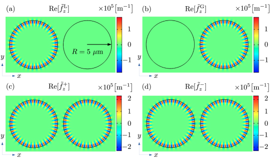
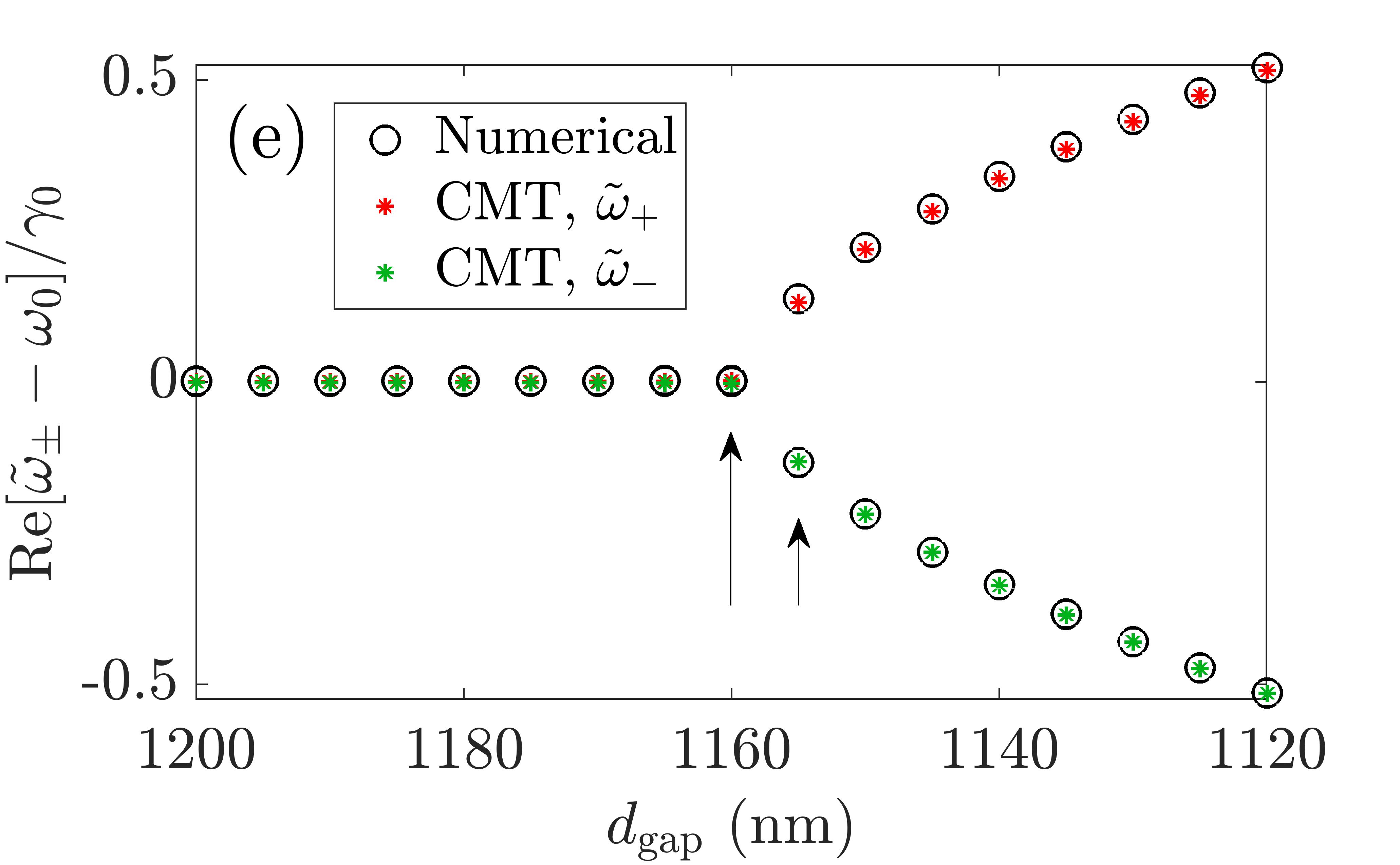
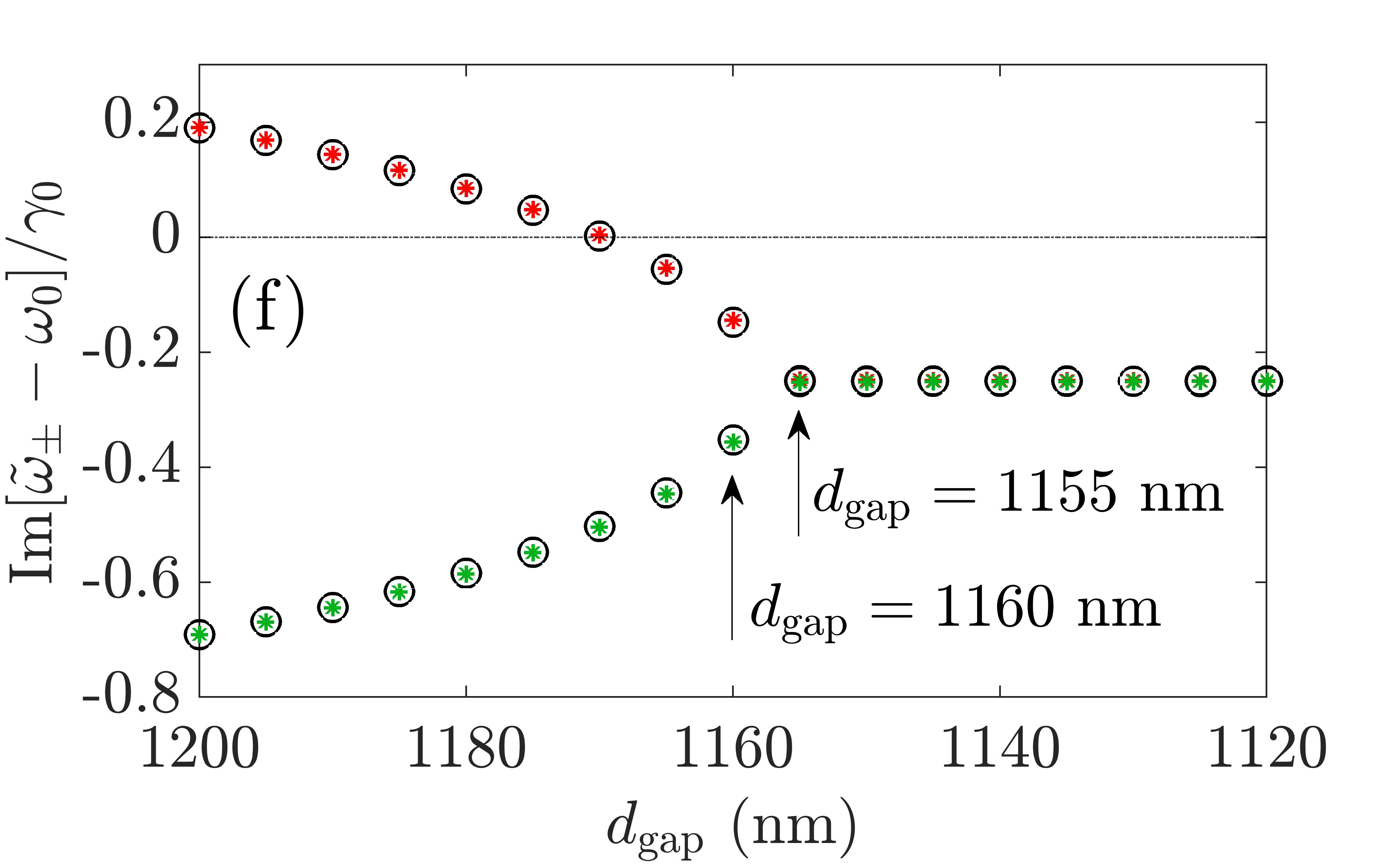
Figure 2: Spatial profile of the QNMs for the following cavity configurations: (a) lossy resonator only (${\rm Re}[\tilde{f}^{\rm L}_{z}]$, Eq. (71)), (b) gain resonator only (${\rm Re}[\tilde{f}^{\rm G}_{z}]$, Eq.(71)), and (c-d) Hybrid modes with coupling (${\rm Re}[\tilde{f}^{\pm}_{z}]$, Eq.(III.4)), for a separation distance $d_{\rm gap}=1155$ nm; this regime is close to the EP as shown in (e) and (f). (e-f) Complex QNM eigenfrequencies of the coupled microdisk resonators from a direct numerical eigenfrequency solver in COMSOL (numerical, black circles) and the analytical CMT (Eq. (30), red stars for $\tilde{\omega}_{+}$, green stars for $\tilde{\omega}_{-}$), as a function of gap separation $d_{\rm gap}$. Note using the eigenfrequency solver, there are two bare degenerate modes per resonator, and four new eigenfrequencies for coupled resonators (four black circles for each gap distance), but with two pair of degenerate modes. For the dipole QNM technique, only one of degenerate standing-wave QNMs are obtained and used for single resonator (see text and Appendix A); thus, the analytical CMT produced two new eigenfrequencies in the presence of finite coupling (one red star and one green star for each gap distance). The arrows show two solutions near an EP. Note that $\omega_{0}$ and $\gamma_{0}$ are for uncoupled single lossy resonator with $n_{\rm loss}=2+10^{-5}i$ ($\tilde{\omega}_{\rm L}=\omega_{\rm L}-i\gamma_{\rm L}=\omega_{0}-i\gamma_{0})$; while for the uncoupled single gain cavity, with $n_{\rm loss}=2-5\times 10^{-6}i$, the resonance is around at $\tilde{\omega}_{\rm G}\approx\omega_{0}+i0.5\gamma_{0}$.

Before investigating the coupled resonator regime, we first show the QNMs for the single loss or gain resonators, which will be used as input for the CMT in the next subsection.

A single 2D microdisk resonator supports WGMs Righini et al. (2011); Schunk et al. (2014), which generally can be described by three integers: radial mode number $q$ (=1,2,3…), azimuthal mode number $m$, and polarization $p$ (TM or TE). Note that for the same $q$, $m$, and $p$, there are two degenerate counterpropagating modes Leung et al. (1994a); Mazzei et al. (2007); Teraoka and Arnold (2009); Cognée et al. (2019): ${E}_{\rm cw}(\mathbf{r},\phi)=E(\mathbf{r})e^{(-im\phi)}$ with clockwise (cw) direction and ${E}_{\rm ccw}(\mathbf{r},\phi)=E(\mathbf{r})e^{(im\phi)}$ with counter clockwise (ccw) direction. for a TM mode, there is only the $z$ component for electric fields), which share the same eigenvalues ( for a TE mode, the $z$ component of the magnetic field has similar properties). A linear combinations of these modes result in degenerate standing waves Mazzei et al. (2007); Teraoka and Arnold (2009); Cognée et al. (2019), such as a symmetric standing mode ${E}_{\rm s}={E}_{\rm cw}+{E}_{\rm ccw}\propto\cos{(m\phi)}$, and an antisymmetric standing wave mode ${E}_{\rm as}={E}_{\rm cw}-{E}_{\rm ccw}\propto\sin{(m\phi)}$.

In general, the mode with $q=1$ and $m\gg 1$ has a high $Q$ and strong field confinement. In this work, we focus on a TM mode (${H}_{x},{H}_{y},{E}_{z}$) with $q=1$, and $m=37$ (yielding a resonant wavelength near the telecommunication band, around $1487\leavevmode\nobreak\$nm). To compute the normalized QNMs, we employ an efficient dipole scattering approach to obtain the QNMs in complex frequency Bai et al. (2013), where an out-of-plane line current (a point in 2D, $z$-polarized) is placed at $10$ nm away from the 2D microdisk (the dipole is at $\mathbf{r}_{\rm d}=\mathbf{r}_{1}$ for the single lossy cavity and at $\mathbf{r}_{\rm d}=\mathbf{r}_{5}$ for the single gain cavity). For more details, see Appendix A.1.

Conveniently, for our TM dipole location along the $x$-axis, we excite only one of the two degenerate standing wave modes, as shown in Fig. 4(a) for the single lossy cavity, which has the form $\cos(m\phi)$ if one considers $\phi=0$ at the positive $x$-axis. The orthogonal and generate QNM has the form $\sin(m\phi)$, constructed from an asymmetric linear combination of the clockwise and counter clockwise modes, though we only need to consider the symmetric QNM for our chosen dipole locations below. More details can be found in Appendix LABEL:sec:degenerate_WGMs. Also note that this working QNM dominates in the frequency region of interest below, because the two closest modes are $q=4$, $m=25$ and $q=3$, $m=29$, and the angular frequency spacing between them and the working mode are $\Delta\omega=3.43{\leavevmode\nobreak\ \rm THz}$ and $\Delta\omega=19.6{\leavevmode\nobreak\ \rm THz}$, which are much larger than the FWHM ($\sim 12.52{\leavevmode\nobreak\ \rm GHz}$ for the single lossy cavity, and $\sim 6.26{\leavevmode\nobreak\ \rm GHz}$ for the single gain cavity). Also note, the free spectral range for modes with $q=1$ is also much larger than these FWHM values, e.g., the angular frequency spacing between $q=1$, $m=36$ (or $q=1$, $m=38$) with the working mode ($q=1$, $m=37$), would be around $\Delta\omega=31.6{\leavevmode\nobreak\ \rm THz}$. Thus, we can adopt a single QNM approximation for the mode of interest for each resonator, which we will also verify below by performing full dipole calculations with no mode approximations.

Numerically, the complex angular eigenfrequency for single lossy resonator is found to be $\tilde{\omega}_{\rm L}=\omega_{\rm L}-i\gamma_{\rm L}\equiv\omega_{0}-i\gamma_{0}=1.266666\times 10^{15}-6.260269\times 10^{9}i$ rad/s, with a quality factor $Q\sim 10^{5}$; here $\omega_{0}$ ($\gamma_{0}$) is the real part (opposite imaginary part) of the complex eigenfrequency. The corresponding QNM field distribution (real part ${\rm Re}[\tilde{f}_{z}^{\rm L}]$), is shown in Fig. 4 (a); the imaginary part is much smaller than the real part, and thus is not shown.

To better understand the overlap integrals for use in CMT, the QNMs at the second resonator region are also shown ($1155\leavevmode\nobreak\$ nm away, i.e., $d_{\rm gap}=1155\leavevmode\nobreak\$nm), which is hardly seen on a linear scale because they are very small compared with fields close to the resonator. This also indicates that the lossy QNMs show no sign of a spatial divergence in this region and thus they can be accurately used for input to CMT, which is a consequence of the high $Q$.

Similarly, the complex angular eigenfrequency for the single gain resonator is found at $\tilde{\omega}_{\rm G}=\omega_{\rm G}-i\gamma_{\rm G}\sim\omega_{0}+i0.5\gamma_{0}$. The corresponding QNM field distribution (real part ${\rm Re}[\tilde{f}_{z}^{\rm G}]$) is shown in Fig. 4(b). In addition, the Purcell factors from the dipole location ($10\leavevmode\nobreak\$nm away from the loss and gain resonator), using a single QNM contribution, (Eq. (5)) agree quantitatively well with full dipole results (see Appendix LABEL:sec:single_modes). We also highlight that the Purcell factors (as defined in a semi-classical model) are net negative for single gain cavity only (since the field is being amplified rather than dissipated), a regime that will also be shown below for the coupled resonator system.

V.2 Hybrid quasinormal modes for coupled loss-gain resonators

We next study the hybrid QNMs formed from the two coupled microdisk resonators, using the QNM CMT and also using full numerical solutions to confirm the accuracy of our semi-analytical results.

Using only the QNMs from single lossy/gain cavities as input, the properties for the coupled modes are obtained analytically. First, the new angular eigenfrequencies $\tilde{\omega}_{\pm}$ are computed from Eq. (30), where the coupling coefficients $\tilde{\kappa}_{12}$ and $\tilde{\kappa}_{21}$ (both complex, Eq. (30)) are related to the overlap QNM integrals for different gap distances $d_{\rm gap}$. Note the input variables $\tilde{\omega}_{1/2}$ and $\tilde{\mathbf{f}}_{1/2}$ in theory parts are changed to $\tilde{\omega}_{\rm L/G}$ and $\tilde{\mathbf{f}}^{\rm L/G}$ in the numerical parts accordingly. As shown in Figs. 4(e) and (f), the analytical eigenfrequencies (Eq. (30)) versus full numerical solution in COMSOL (eigenfrequency solver) show excellent agreement, and at all gap separations. This quantitative level of agreement is also obtained for the QNMs and the QNM Green functions as we will show in more detail below.

The complex coupling coefficients for $d_{\rm gap}=1155\leavevmode\nobreak\$nm ($d_{\rm gap}=1160\leavevmode\nobreak\$nm) are $\tilde{\kappa}_{12}/\gamma_{0}=-0.7614-5.745\times 10^{-6}i$ ($-0.7425-5.375\times 10^{-6}i$) and $\tilde{\kappa}_{21}/\gamma_{0}=-0.7425+4.153\times 10^{-5}i$ ($-0.7425+4.087\times 10^{-6}i$), where the small imaginary part is mainly due to the high quality factor of the bare resonator and one can find they do not satisfy $\tilde{\kappa}_{12}=\tilde{\kappa}_{21}^{*}$ in general, as mentioned in Sec. III.3. This is also true for balanced loss-gain systems, and these inconspicuous imaginary parts would affect the condition for finding a perfect EP, e.g., as in Ref. Chen et al. (2018).

Note, with a direct QNM eigenfrequency solver, there would be four new eigenfrequencies for coupled resonators, because there are two degenerate standing modes per resonator (see Appendix LABEL:sec:degenerate_WGMs); thus, there are four black circles for each gap distance in Fig. 4 (e) and (f), but with two pairs of degenerate modes. In contrast, with QNM dipole technique (see Appendix A), only one of the degenerate standing modes are used. Hence, when combining with the analytical CMT approach, there are only two new eigenfrequencies for coupled resonators – labelled by the red star and the green star for each gap distance in Fig. 4(e) and (f).

Equation (III.4) gives the two new coupled QNMs $\tilde{\mathbf{f}}^{\pm}$ (hybrid QNMs) corresponding to the two new eigenfrequencies $\tilde{\omega}_{\pm}$, where the input fields $\tilde{\mathbf{f}}_{1}$ and $\tilde{\mathbf{f}}_{2}$ are now $\tilde{\mathbf{f}}^{\rm L}$ and $\tilde{\mathbf{f}}^{\rm G}$. The spatial profile of the coupled QNMs (real part ${\rm Re}[\tilde{f}^{\pm}_{z}]$) for $d_{\rm gap}=1155\leavevmode\nobreak\$nm are shown in Figs. 4 (c) and (d), where the fields now extend over both resonators. Below we study two example gap cases close to the lossy EP, namely $d_{\rm gap}=1155\leavevmode\nobreak\$nm and $d_{\rm gap}=1160\leavevmode\nobreak\$nm, indicated by the arrows in Figs. 4(e) and (f).

V.3 Non-Lorentzian Purcell factors close to a lossy exceptional point: Quasinormal mode Green function solution versus full dipole simulations

Next, we focus on the Purcell factors close to the lossy EPs in the coupled loss-gain resonators. Once the coupled QNMs (Eq. (III.4)) are obtained from CMT (the input fields $\tilde{\mathbf{f}}_{1}$ and $\tilde{\mathbf{f}}_{2}$ are now $\tilde{\mathbf{f}}^{\rm L}$ and $\tilde{\mathbf{f}}^{\rm G}$), the generalized Purcell factors are obtained analytically from Eq. (5), using the QNM Green function (Eq. (34)). As shown in Fig. 1, we consider five potential dipole positions along the $x$-axis, and study the Purcell factors as a function of frequency in each case.

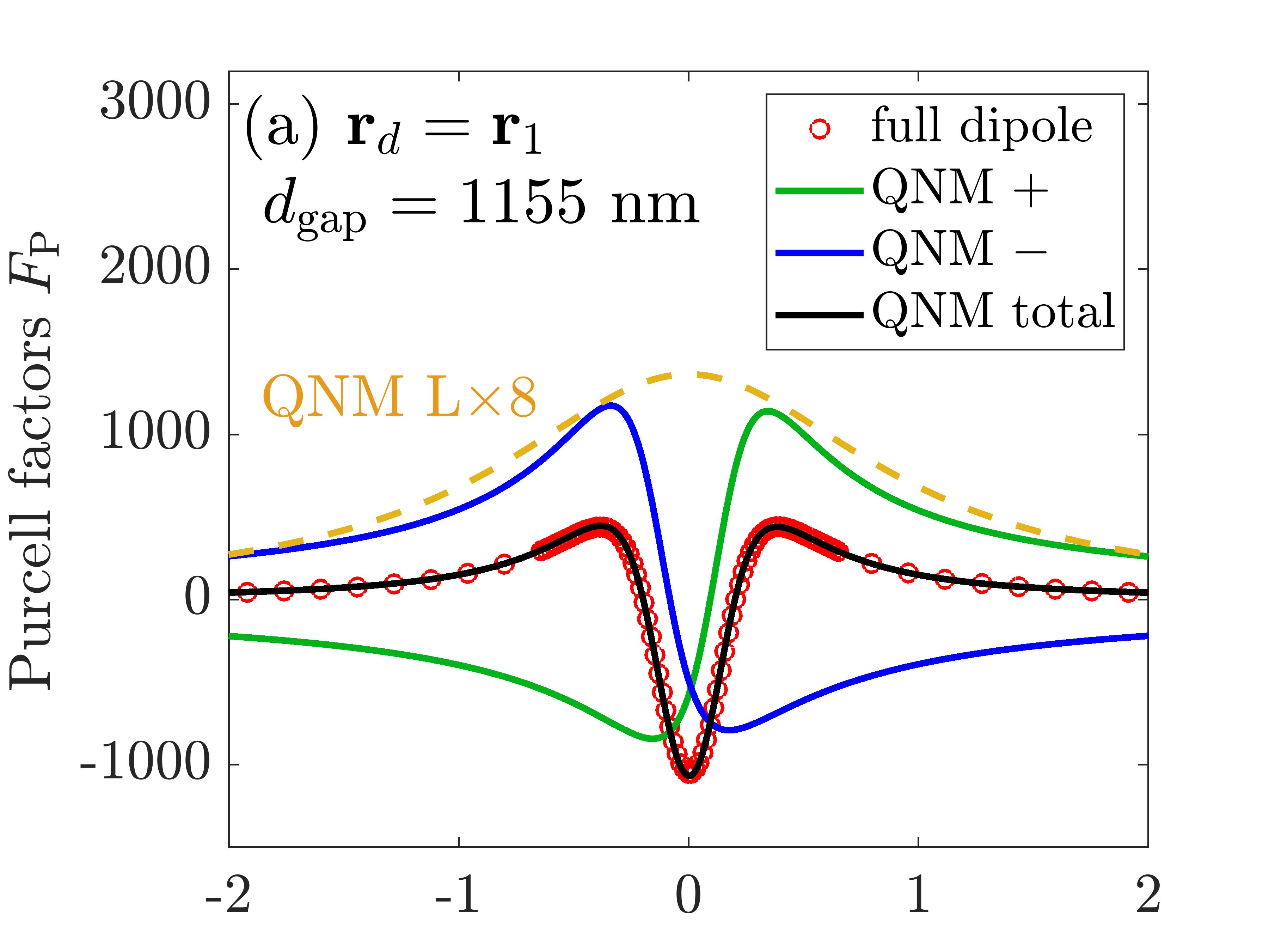
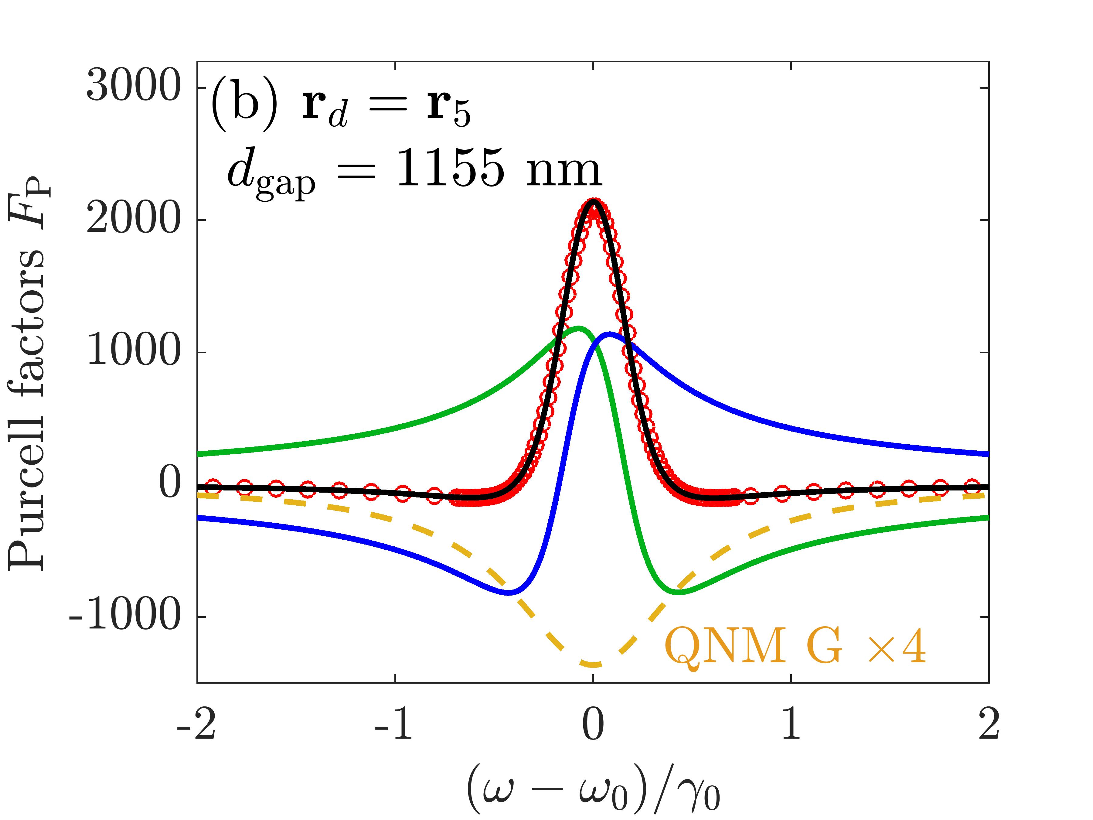
Figure 3: (a) Purcell factors for the coupled resonators with gap distance $d_{\rm gap}=1155\leavevmode\nobreak\$nm, showing the analytical CMT solutions ((Eq. (34) and Eq. (5) or Eq. (LABEL:eq:2Dpurcell))) for the hybrid QNM contributions as well as their sum. Also shown is the full dipole simulation with no approximations (red marker, Eq. (LABEL:Purcellfulldipole)), and the QNM contribution from a single lossy resonator (multiplied by a constant for clarity). The dipole is placed at $\mathbf{r}_{\rm d}=\mathbf{r}_{1}$ ($10\leavevmode\nobreak\$ nm away from the lossy resonator). (b) Similar to (a), but with a different dipole position $\mathbf{r}_{\rm d}=\mathbf{r}_{5}$, $10\leavevmode\nobreak\$nm away from the gain resonator.

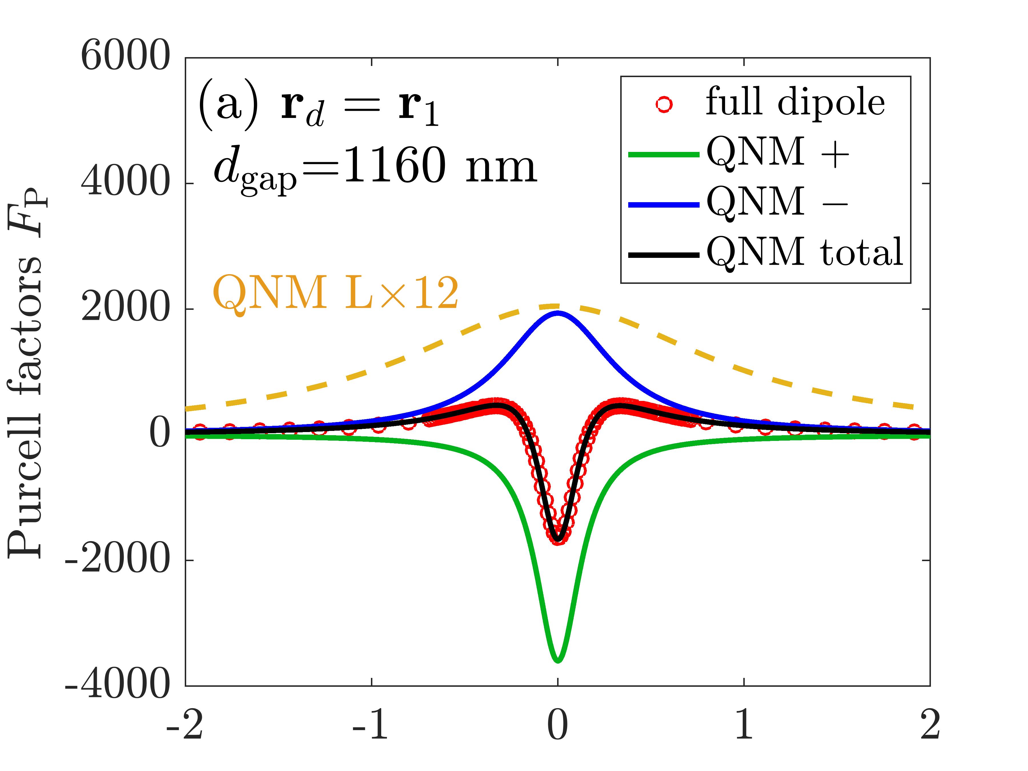
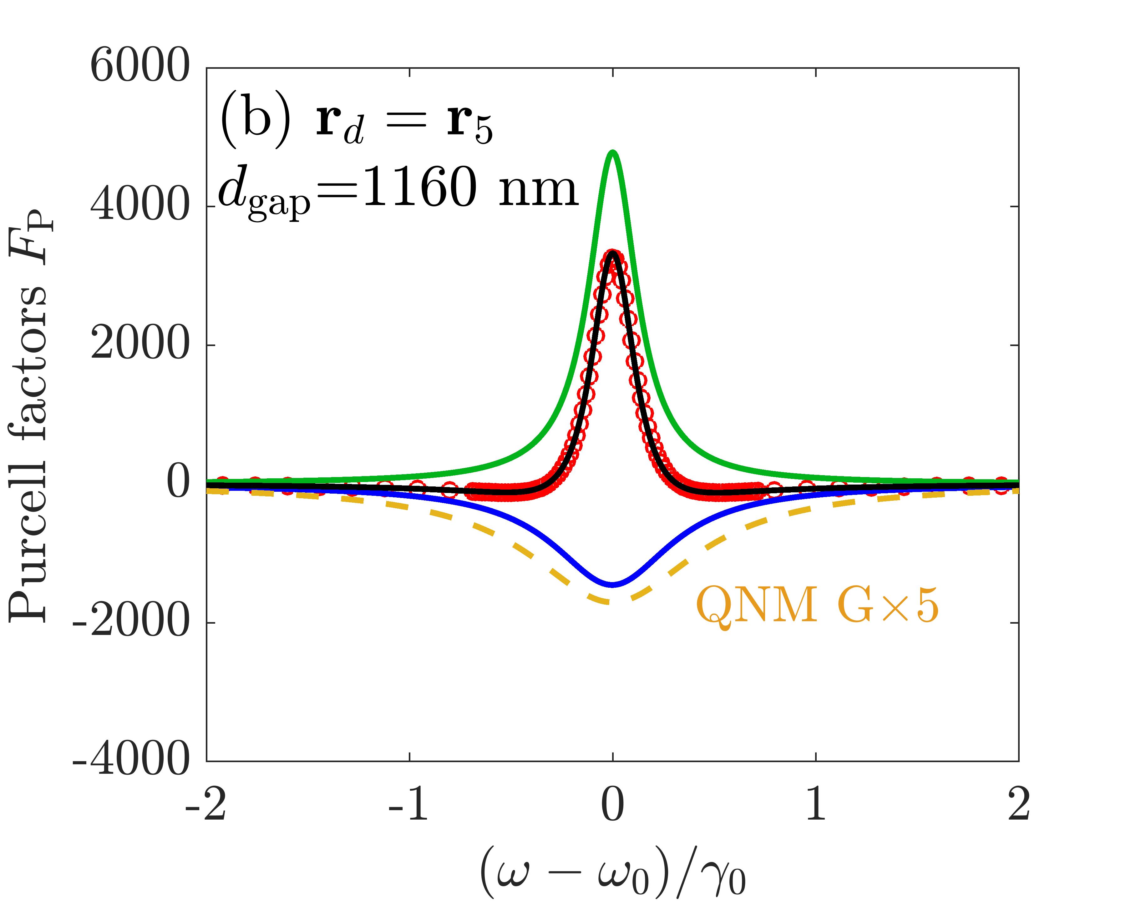
Figure 4: Similar to Fig. 3, but with a different gap distance $d_{\rm gap}=1160\leavevmode\nobreak\$nm.

For a dipole at the position $\mathbf{r}_{\rm d}=\mathbf{r}_{1}$ ($10\leavevmode\nobreak\$nm away from the lossy cavity), the Purcell factors are shown in Fig. 3(a) with $d_{\rm gap}=1155\leavevmode\nobreak\$nm, where negative Purcell factors (black solid curve) are found in a wide range of frequencies. The black solid line shows the analytical QNM Green function result using only the bare resonator parameters as input, and the red circles show full dipole solutions, showing quantitatively good agreement over all frequencies. We stress there are no fitting parameters in the QNM solutions. Moreover, from our theory, the contribution from the hybrid QNMs $\tilde{f}^{+}$ and $\tilde{f}^{-}$ can be shown separately, as indicated by the green and blue solid curves (Eq. (34), the first and second term). As a reference, we also show the Purcell factors for a single lossy cavity (orange dashed curve), which is net positive and multiplied by $8$ for a better graphical comparison. The gain resonator clearly acts to suppress the broadening and enhance the overall Purcell factors.

Table 1: Phase contributions in the imaginary part of QNM Green function, which is used to explain the lineshapes of the corresponding Purcell factors shown in Fig. 3 and Fig. 4.

	$\mathbf{r}_{\rm d}=\mathbf{r}_{1}$	$\mathbf{r}_{\rm d}=\mathbf{r}_{5}$
QNM L	$\cos{(2\phi^{\rm L})}=1.0000$, $\sin{(2\phi^{\rm L})}=-0.0012$
QNM G		$\cos{(2\phi^{\rm G})}=1.0000$, $\sin{(2\phi^{\rm G})}=0.0005$
$d_{\rm gap}=1155\leavevmode\nobreak\$nm	$\cos{(2\phi^{+})}=0.1514$, $\sin{(2\phi^{+})}=-0.9885$	$\cos{(2\phi^{+})}=0.1834$, $\sin{(2\phi^{+})}=0.9830$
	$\cos{(2\phi^{-})}=0.1939$, $\sin{(2\phi^{-})}=0.9810$	$\cos{(2\phi^{-})}=0.1620$, $\sin{(2\phi^{-})}=-0.9868$
$d_{\rm gap}=1160\leavevmode\nobreak\$nm	$\cos{(2\phi^{+})}=-1.0000$, $\sin{(2\phi^{+})}=0.0009$	$\cos{(2\phi^{+})}=0.9999$, $\sin{(2\phi^{+})}=0.0101$
	$\cos{(2\phi^{-})}=1.0000$, $\sin{(2\phi^{-})}=-0.0011$	$\cos{(2\phi^{-})}=-0.9999$, $\sin{(2\phi^{-})}=-0.0129$

To help explain these unusual lineshapes, we can study the contributions to the QNM Green functions from the phases for the two hybrid QNMs. Defining $\tilde{f}^{+}_{z}(\mathbf{r})=|\tilde{f}^{+}_{z}(\mathbf{r})|e^{i\phi^{+}(\mathbf{r})}$ and $\tilde{f}^{-}_{z}(\mathbf{r})=|\tilde{f}^{-}_{z}(\mathbf{r})|e^{i\phi^{-}(\mathbf{r})}$, the QNM Green function can be expressed as

$${G}_{zz}(\mathbf{r}_{\rm d},\mathbf{r}_{\rm d},\omega)=$$

$$\ =A^{+}(\omega)\tilde{f}^{+}_{z}(\mathbf{r}_{\rm d})\tilde{f}^{+}_{z}(\mathbf{r}_{\rm d})+A^{-}(\omega)\tilde{f}^{-}_{z}(\mathbf{r}_{\rm d})\tilde{f}^{-}_{z}(\mathbf{r}_{\rm d})$$

$$\ =A^{+}(\omega)e^{i2\phi^{+}(\mathbf{r}_{\rm d})}|\tilde{f}^{+}_{z}(\mathbf{r}_{\rm d})|^{2}+A^{-}(\omega)e^{i2\phi^{-}(\mathbf{r}_{\rm d})}|\tilde{f}^{-}_{z}(\mathbf{r}_{\rm d})|^{2},$$ (48)

from which we extract the imaginary part for use in Purcell’s formula El-Sayed and Hughes (2020):

$$\begin{split}&{\rm Im}[{G}_{zz}(\mathbf{r}_{\rm d},\mathbf{r}_{\rm d},\omega)]\\ =&\bigg{[}\cos{2\phi^{+}(\mathbf{r}_{\rm d})}+\frac{\omega_{+}-\omega}{\gamma_{+}}\sin{2\phi^{+}(\mathbf{r}_{\rm d})}\bigg{]}\Big{|}\tilde{f}^{+}_{z}(\mathbf{r}_{\rm d})\Big{|}^{2}L^{+}(\omega)\\ +&\bigg{[}\cos{2\phi^{-}(\mathbf{r}_{\rm d})}+\frac{\omega_{-}-\omega}{\gamma_{-}}\sin{2\phi^{-}(\mathbf{r}_{\rm d})}\bigg{]}\Big{|}\tilde{f}^{-}_{z}(\mathbf{r}_{\rm d})\Big{|}^{2}L^{-}(\omega),\end{split}$$ (49)

where we introduced the normalized Lorentzian lineshapes,

$$L^{+}(\omega) =\frac{\omega}{2}\frac{\gamma_{+}}{(\omega_{+}-\omega)^{2}+\gamma_{+}^{2}},$$

$$L^{-}(\omega) =\frac{\omega}{2}\frac{\gamma_{-}}{(\omega_{-}-\omega)^{2}+\gamma_{-}^{2}},$$ (50)

with $\tilde{\omega}_{+}=\omega_{+}-i\gamma_{+}$, $\tilde{\omega}_{-}=\omega_{-}-i\gamma_{-}$, $A^{+}(\omega)=\omega/[2(\tilde{\omega}_{+}-\omega)]$, and $A^{-}(\omega)=\omega/[2(\tilde{\omega}_{-}-\omega]$. Similar expressions have been used to explain Fano resonances formed by elastic QNMs in coupled cavity beams El-Sayed and Hughes (2020).

For comparison, the Green functions for the single-mode bare QNMs are also given as

$$\begin{split}&{\rm Im}[{G}_{zz}^{\rm L}(\mathbf{r}_{\rm d},\mathbf{r}_{\rm d},\omega)]\\ =&\bigg{[}\cos{2\phi^{\rm L}(\mathbf{r}_{\rm d})}+\frac{\omega_{1}-\omega}{\gamma_{1}}\sin{2\phi^{\rm L}(\mathbf{r}_{\rm d})}\bigg{]}\Big{|}\tilde{f}^{\rm L}_{z}(\mathbf{r}_{\rm d})\Big{|}^{2}L^{\rm L}(\omega),\end{split}$$ (51)

$$\begin{split}&{\rm Im}[{G}_{zz}^{\rm G}(\mathbf{r}_{\rm d},\mathbf{r}_{\rm d},\omega)]\\ =&\bigg{[}\cos{2\phi^{\rm G}(\mathbf{r}_{\rm d})}+\frac{\omega_{2}-\omega}{\gamma_{2}}\sin{2\phi^{\rm G}(\mathbf{r}_{\rm d})}\bigg{]}\Big{|}\tilde{f}^{\rm G}_{z}(\mathbf{r}_{\rm d})\Big{|}^{2}L^{\rm G}(\omega),\end{split}$$ (52)

with normalized Lorentzian lineshapes for the loss and gain resonator modes, and we have redefined the QNMs as $\tilde{f}^{\rm L}_{z}(\mathbf{r})=|\tilde{f}^{\rm L}_{z}(\mathbf{r})|e^{i\phi^{\rm L}(\mathbf{r})}$ and $\tilde{f}^{\rm G}_{z}(\mathbf{r})=|\tilde{f}^{\rm G}_{z}(\mathbf{r})|e^{i\phi^{\rm G}(\mathbf{r})}$.

In Fig. 3(a), we show the total Purcell factors for $d_{\rm gap}=1155\leavevmode\nobreak\$nm, as well as the hybrid mode contributions, and the lossy mode result on its own for comparison. First, the single mode case (orange dashed curve, single lossy resonator) shows a typical Lorentzian peak, which can be explained by the QNM phase contributions: $\cos{[2\phi^{\rm L}(\mathbf{r}_{1})]}=0.999999$ and $\sin{[2\phi^{\rm L}(\mathbf{r}_{1})]}=-0.001244$ (also shown in Table  1). Applying these to Eq. (LABEL:Eq:G_loss_phase) results in a typical Lorentzian lineshape.

Next we focus on the hybrid modes (coupled resonator case), where now: $\cos{[2\phi^{+}(\mathbf{r}_{1})]}=0.1514$, $\sin{[2\phi^{+}(\mathbf{r}_{1})]}=-0.9885$, and $\cos{[2\phi^{-}(\mathbf{r}_{1})]}=0.1939$, $\sin{[2\phi^{-}(\mathbf{r}_{1})]}=0.9810$ (also shown in Table 1), which explain the non-Lorentzian lineshapes for the separate contributions (two terms in Eq. (49), green solid curve and blue solid curve shown in Fig. 3 (a)). Then combining the weights for each term (from $|\tilde{f}^{+}_{z}(\mathbf{r}_{1})|^{2}$ and $|\tilde{f}^{-}_{z}(\mathbf{r}_{1})|^{2}$ as shown in Eq. (49)), we obtain negative Purcell factors in a wide range of frequencies (black solid curve in Fig. 3 (a)).

Furthermore, these QNM phases will result in position-dependent lineshapes for the Purcell factors. Thus when we change the dipole position from $\mathbf{r}_{\rm d}=\mathbf{r}_{1}$ to $\mathbf{r}_{\rm d}=\mathbf{r}_{5}$ ($10\leavevmode\nobreak\$nm away from the gain cavity), the Purcell factor lineshapes can change significantly, as shown in Fig. 3 (b) (again for $d_{\rm gap}=1155\leavevmode\nobreak\$nm), where the total contribution (black solid curve) are found to be mainly net positive in a wide range of frequency, and also show excellent agreement with the full dipole method (red circles). Once again, the contribution from $\tilde{f}^{+}$ and $\tilde{f}^{-}$ can be given separately, as shown with the green and blue solid curves. In addition, the Purcell factors for the single gain cavity is shown as an orange dashed curve, which is net negative (and multiplied by $4$ for a better graphical comparison).

As before, these lineshapes can also be well explained from the QNM phase terms. For a single gain cavity, one finds that $\cos{[2\phi^{\rm G}(\mathbf{r}_{5})]}=0.999999$ and $\sin{[2\phi^{\rm G}(\mathbf{r}_{5})]}=0.000527$ (also shown in Table  1). However, with $\gamma_{\rm G}<0$, then $L^{\rm G}(\omega)$ shows a negative Lorentzian lineshape, yielding negative Purcell factors with the gain cavity only (orange dashed curve in Fig. 3(b)). As for the coupled system, one can find $\cos{[2\phi^{+}(\mathbf{r}_{5})]}=0.1834$, $\sin{[2\phi^{+}(\mathbf{r}_{5})]}=0.9830$, and $\cos{[2\phi^{-}(\mathbf{r}_{5})]}=0.1620$, $\sin{[2\phi^{-}(\mathbf{r}_{5})]}=-0.9868$ (also shown in Table  1), which explain the non-Lorentzian lineshapes for separate contribution (two terms in Eq. (49), green solid curve and blue solid curve shown in Fig. 3 (b)). Then combining the weights for each term (from $|\tilde{f}^{+}_{z}(\mathbf{r}_{5})|^{2}$ and $|\tilde{f}^{-}_{z}(\mathbf{r}_{5})|^{2}$ in Eq. (49)), the mostly positive Purcell factors are obtained (black solid curve in Fig. 3(b)).

Similar to case with a gap distance $d_{\rm gap}=1155\leavevmode\nobreak\$nm, the Purcell factors with $d_{\rm gap}=1160\leavevmode\nobreak\$nm for a dipole at $\mathbf{r}_{1}$ are shown in Fig. 4(a). Their separate contributions from ${\rm QNM}\leavevmode\nobreak\ +$ (green solid curve) and ${\rm QNM}\leavevmode\nobreak\ -$ (blue solid curve) show Lorentzian lineshapes, but with different linewidth since $\gamma_{+}\neq\gamma_{-}$ (see Fig. 4 (f)) and different signs due to $\cos{[2\phi^{+}(\mathbf{r}_{1})]}=-1.0000$ and $\cos{[2\phi^{-}(\mathbf{r}_{1})]}=1.0000$. Combing these contributions, the total contribution are found to be net negative in a wide range of frequencies. When the dipole is at $\mathbf{r}_{5}$, the Purcell factors are shown in Fig. 4 (b), where the Lorentzian lineshapes for separate contributions could also be explained by the QNM phases $\cos{[2\phi^{+}(\mathbf{r}_{5})]}=0.9999$ and $\cos{[2\phi^{-}(\mathbf{r}_{5})]}=-0.9999$. Considering their separate contributions, the total Purcell factors are now mostly positive. More details about the QNM phases are shown in Table 1.

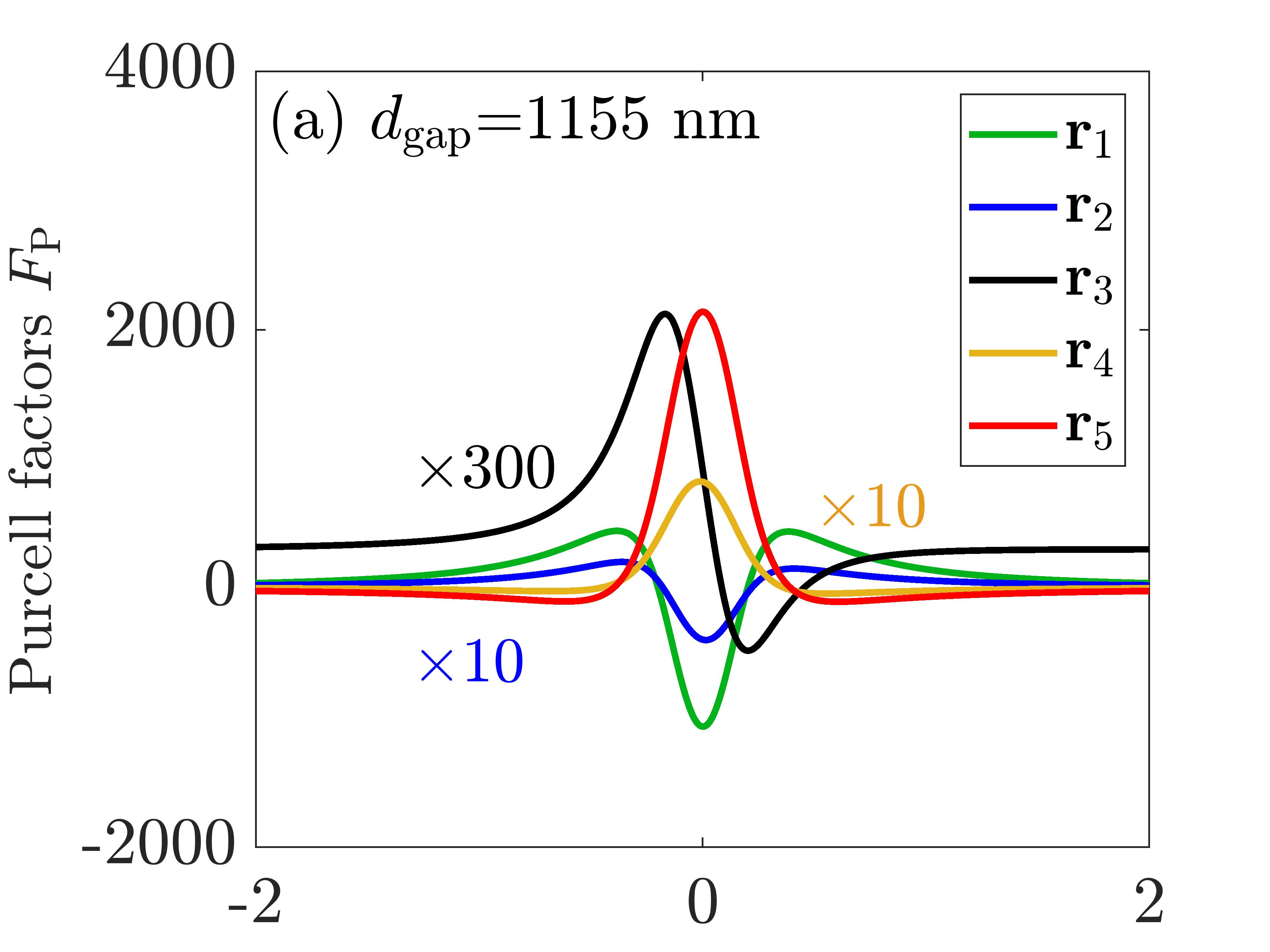
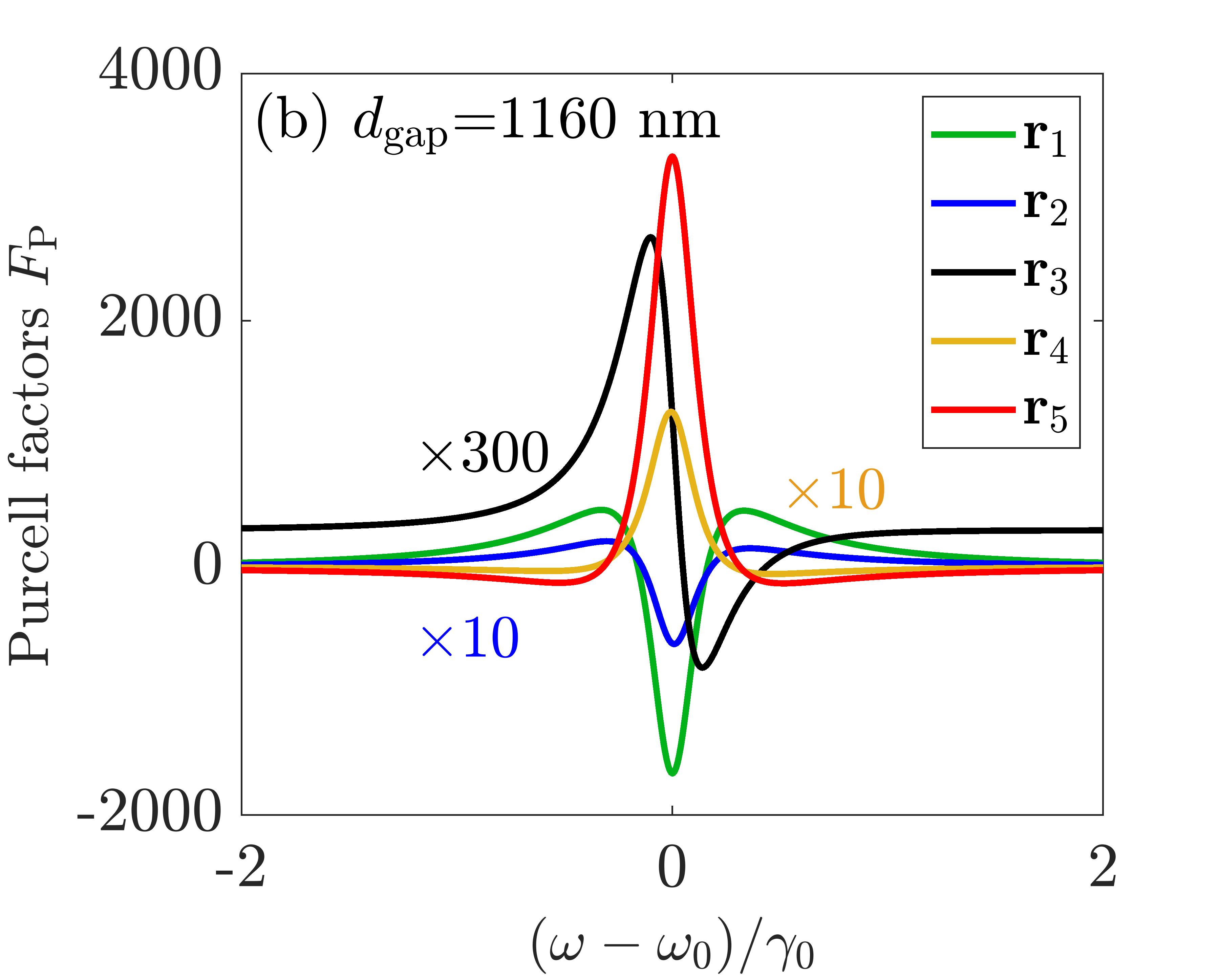
Figure 5: Purcell factors at different dipole positions $\mathbf{r}_{\rm d}=\mathbf{r}_{1}\sim{\bf r}_{5}$ (shown in Fig. 1), for two different gap separations (a) $d_{\rm gap}=1155\leavevmode\nobreak\$nm, and (b) $d_{\rm gap}=1160\leavevmode\nobreak\$nm. Full dipole simulations are not shown for clarity, but yield the same quantitatively good fit as in the previous graphs.

These QNM phases have a significant effect on the spectral lineshapes of the Purcell factors, which can be further seen in Fig. 5(a) (for $d_{\rm gap}=1155\leavevmode\nobreak\$nm) and (b) (for $d_{\rm gap}=1160\leavevmode\nobreak\$nm), where the total Purcell factors are given for five different dipole positions as shown in Fig. 1. For better comparison, the Purcell factors at $\mathbf{r}_{2}$, $\mathbf{r}_{3}$ and $\mathbf{r}_{4}$ are multiplied by $10$, $300$ and $10$. Note, we do not show the full dipole results here, as they are basically indistinguishable from the the two QNM solutions, similar to the previous comparisons.

We stress that these negative Purcell factors are unphysical because the classical Purcell factor formulas, and Fermi’s golden rule, is no longer working with a gain medium Franke et al. (2021), though the local density of states (LDOS, proportional to ${\rm Im}[\mathbf{G}(\mathbf{r}_{\rm d},\mathbf{r}_{\rm d},\omega)]$) is correct. Reference  Franke et al., 2021 discusses the breakdown of classical formulas in more detail, and shows that the correct SE rates must be described fully quantum mechanically, in which case the quantum Purcell factors (modified SE decay rayes) are indeed net positive.

V.4 Green function Propagators

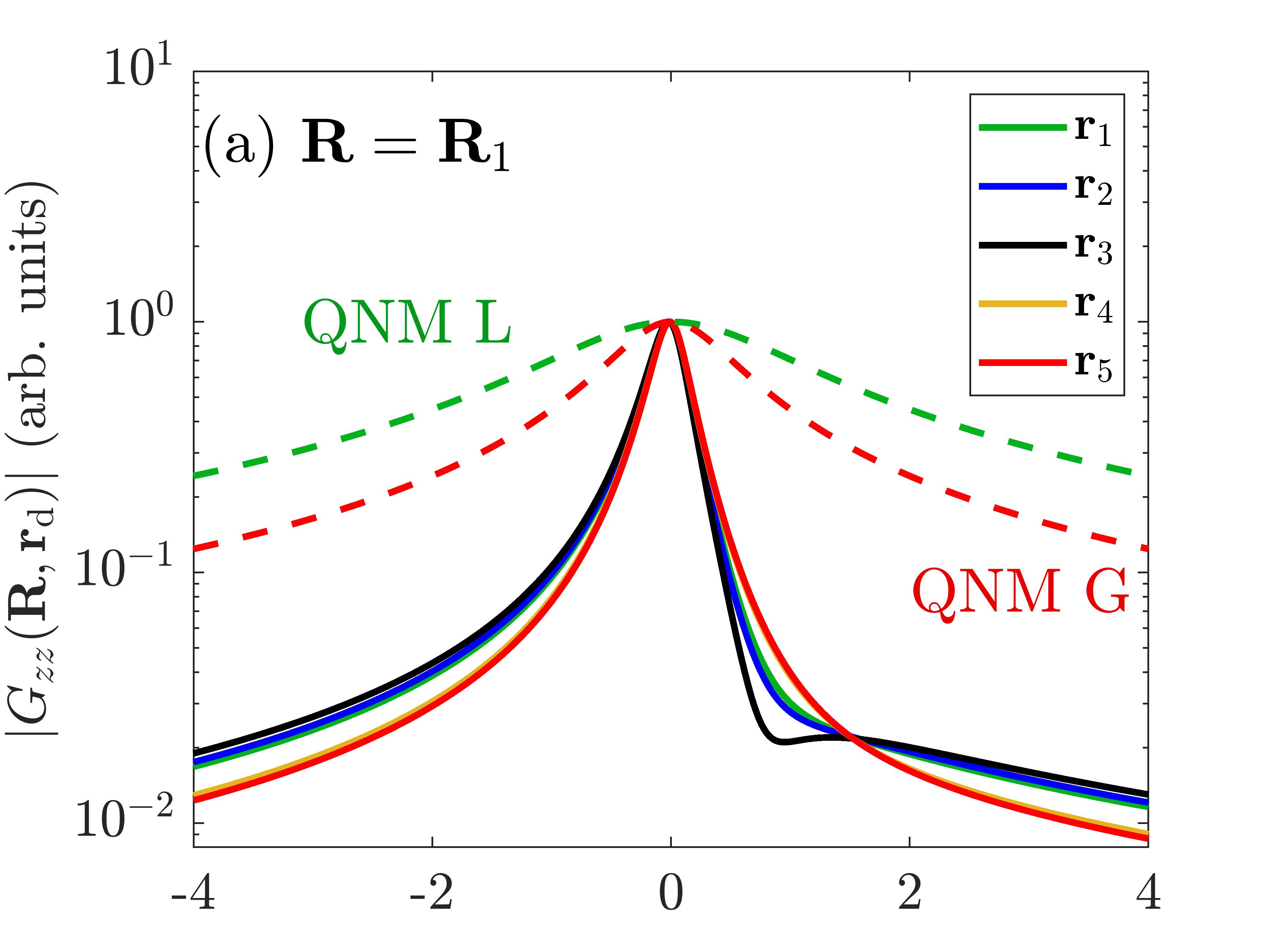
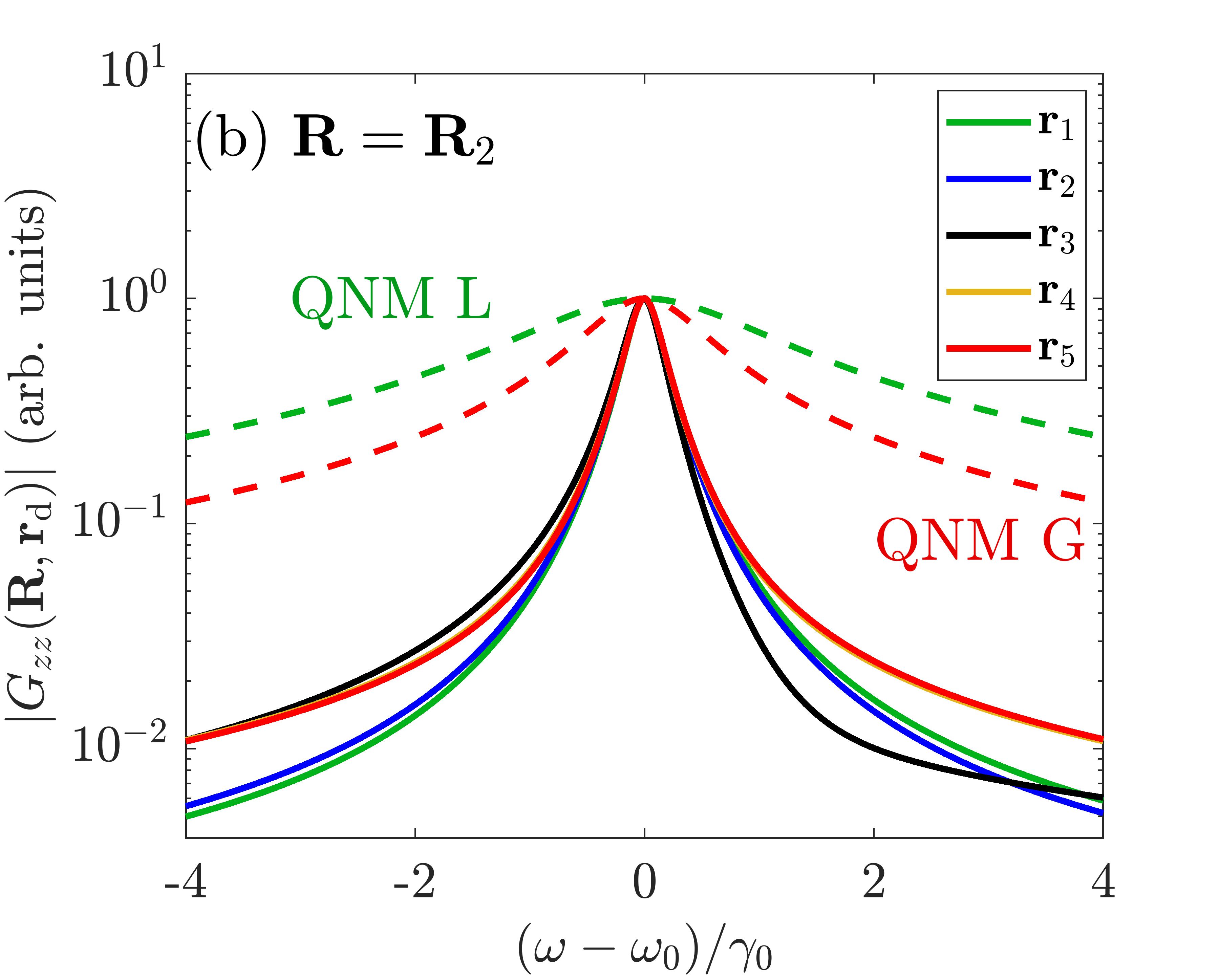
Figure 6: Green function propagator for the far field detected point is at (a) $\mathbf{R}=\mathbf{R}_{1}=$[0,10] $\mu$m, and (b) $\mathbf{R}=\mathbf{R}_{2}=[14.09,0]\leavevmode\nobreak\ \mu$m (which is $3.51\leavevmode\nobreak\ \mu$m away from the gain cavity) with $d_{\rm gap}=1160\leavevmode\nobreak\$nm. For QNM L (loss), the dipole is at $\mathbf{r}_{\rm d}=\mathbf{r}_{1}$, and for QNM G (gain), it is at $\mathbf{r}_{\rm d}=\mathbf{r}_{5}$. The results for $d_{\rm gap}=1155\leavevmode\nobreak\$nm look similar and we do not show them.

Table 2: Phase contributions from the QNMs in the propagator (Eq. (62)).

	$\mathbf{R}=\mathbf{R}_{1}$	$\mathbf{R}=\mathbf{R}_{2}$
QNM L	$\cos{[\phi^{\rm L}(\mathbf{R})+\phi^{\rm L}(\mathbf{r}_{\rm d})]}=-0.6905$	$-0.9989$
$\mathbf{r}_{\rm d}=\mathbf{r}_{1}$	$\sin{[\phi^{\rm L}(\mathbf{R})+\phi^{\rm L}(\mathbf{r}_{\rm d})]}=0.7234$	$-0.0470$
QNM G	$\cos{[\phi^{\rm G}(\mathbf{R})+\phi^{\rm G}(\mathbf{r}_{\rm d})]}=-0.7036$	$0.2606$
$\mathbf{r}_{\rm d}=\mathbf{r}_{1}$	$\sin{[\phi^{\rm G}(\mathbf{R})+\phi^{\rm G}(\mathbf{r}_{\rm d})]}=0.7106$	$-0.9655$
$d_{\rm gap}=1160\leavevmode\nobreak\$nm	$\cos{[\phi^{+}(\mathbf{R})+\phi^{+}(\mathbf{r}_{\rm d})]}=-0.0815$	$0.9760$
	$\sin{[\phi^{+}(\mathbf{R})+\phi^{+}(\mathbf{r}_{\rm d})]}=-0.9967$	$0.2177$
$\mathbf{r}_{\rm d}=\mathbf{r}_{1}$	$\cos{[\phi^{-}(\mathbf{R})+\phi^{-}(\mathbf{r}_{\rm d})]}=-0.0575$	$-0.9784$
	$\sin{[\phi^{-}(\mathbf{R})+\phi^{-}(\mathbf{r}_{\rm d})]}=0.9983$	$-0.2070$

This next section presents example Green function propagator results, namely $|\mathbf{G}(\mathbf{R},\mathbf{r}_{\rm d},\omega)|$, which can be useful to relate to a range of experimental observables. For example, this function is required to model the spectrum at a point detector located at ${\bf R}$, emitted from a dipole at ${\bf r}_{\rm d}$. Unlike the (classical) Purcell factor, it is a well defined quantity for use in both classical and quantum field theory, and is used frequently in the exploration of light-matter coupling regimes Wubs et al. (2004); Van Vlack et al. (2012); Ge et al. (2013). For example, considering an excitation dipole, ${\bf d}$, then the spectrum is $S({\bf R},\omega)\propto|{\bf G}({\bf R},{\bf r}_{\rm d},\omega)\cdot{\bf d}|^{2}$.

A far-field detection point is first chosen at $\mathbf{R}=\mathbf{R}_{1}=[0,10]\leavevmode\nobreak\ \mu$m (the origin of the coordinate system is at the gap center). The corresponding propagators $|G_{zz}(\mathbf{R},\mathbf{r}_{\rm d},\omega)|$ (arbitrary units) for various dipole positions $\mathbf{r}_{\rm d}$ are shown in Fig. 6(a), for $d_{\rm gap}=1160\leavevmode\nobreak\$nm. For comparison, the propagator for a single lossy (gain) cavity is also shown as green (red) dashed curve, where the dipole is placed at $\mathbf{r}_{\rm d}=\mathbf{r}_{1}$ ($\mathbf{r}_{5}$). Furthermore, for the far field detected point at $\mathbf{R}=\mathbf{R}_{2}=[14.09,0]\leavevmode\nobreak\ \mu$m, the propagators are shown in Fig. 6(b).

To better explain the physics of the propagator lineshape, we once more write out the two QNM expanded Green function in terms of the hybrid modes,

$$\begin{split}&G_{zz}(\mathbf{R},\mathbf{r}_{\rm d},\omega)\\ &=A^{+}(\omega)\tilde{f}^{+}_{z}(\mathbf{R})\tilde{f}^{+}_{z}(\mathbf{r}_{\rm d})+A^{-}(\omega)\tilde{f}^{-}_{z}(\mathbf{R})\tilde{f}^{-}_{z}(\mathbf{r}_{\rm d})\\ &=A^{+}(\omega)e^{i(\phi^{+}(\mathbf{R})+\phi^{+}(\mathbf{r}_{\rm d}))}|\tilde{f}^{+}_{z}(\mathbf{R})||\tilde{f}^{+}_{z}(\mathbf{r}_{\rm d})|\\ &+A^{-}(\omega)e^{i(\phi^{-}(\mathbf{R})+\phi^{-}(\mathbf{r}_{\rm d}))}|\tilde{f}^{-}_{z}(\mathbf{R})||\tilde{f}^{-}_{z}(\mathbf{r}_{\rm d})|,\end{split}$$ (62)

where again we can recognize non-Lorentzian features from the QNM phase terms, now from both the dipole position and the detector position. The detailed phases are shown in Table 2. Note, the two-space point Green function has a range of uses for describing light-matter interactions, including the description of photon transport Wubs et al. (2004); Kristensen et al. (2011); Ge and Hughes (2015), and can be used to model collective effects with multiple emitters and dipoles.

VI Quasinormal modes for index-modulated ring resonators near exceptional points

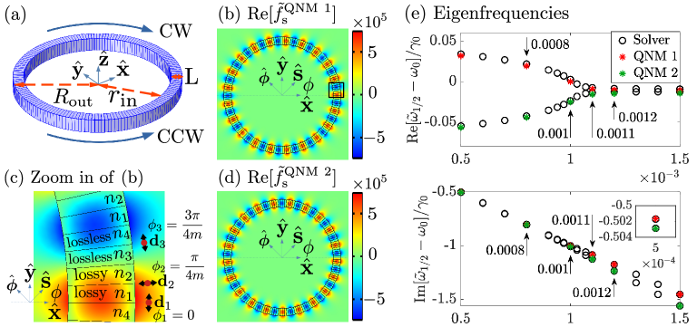
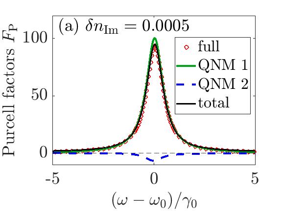
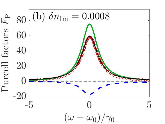
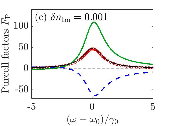
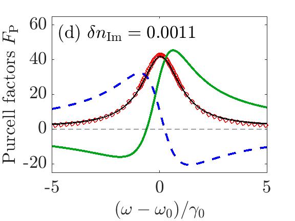
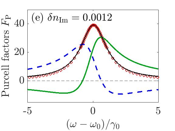
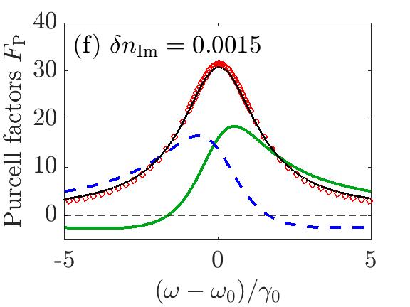
Figure 7: (a) Schematic of the refractive-index-modulated ring resonator. The wo blue arrows label the direction of CW and CCW of the fields. The inner and outer radius (two red dashed arrows) of the ring are $r_{\rm in}=1109\leavevmode\nobreak\$ nm and $R_{\rm out}=1271\leavevmode\nobreak\$nm (width of the ring is ${\rm L}=R_{\rm out}-r_{\rm in}=162\leavevmode\nobreak\$nm). In our calculations, we investigate a 2D ring resonator and couple it with an in-plane linear dipole. The ring is divided into $8m$ ($m=21$) sections, where the refractive indices are $n_{1/2/3/4}$, which are distributed periodically along the CCW direction (see (c)). Field distribution ${\rm Re}[\tilde{f}_{s}]$ (with units $m^{-1}$) ($\tilde{\bf f}=\tilde{f}_{x}\hat{\bf x}+\tilde{f}_{y}\hat{\bf y}=\tilde{f}_{s}\hat{\bf s}+\tilde{f}_{\phi}\hat{\bm{\phi}}$) of (b) QNM 1 and (d) QNM 2 for ring structures with $\delta n_{\rm Re}=\delta n_{\rm Im}=0.001$. (c) Zoom in of the black square in (b). In addition to general unit vectors $\hat{\bf x}$ and $\hat{\bf y}$, we also utilize $\hat{\bf s}=\hat{\bf x}\cos{\phi}+\hat{\bf y}\sin{\phi}$ and $\hat{\bm{\phi}}=-\hat{\bf x}\sin{\phi}+\hat{\bf y}\cos{\phi}$. Three example dipoles are shown, where one ($\mathbf{d}_{1}$) is a linear $\hat{\bm{\phi}}$ dipole at $\phi=\phi_{1}=0$ (i.e., $\hat{\bf y}$ dipole at $\phi=0$), one ($\mathbf{d}_{2}$) is a linear $\hat{\bf s}$ dipole at $\phi=\phi_{2}=\pi/4m$, and the left one ($\mathbf{d}_{3}$) is a linear $\hat{\bm{\phi}}$ dipole at $\phi=\phi_{2}=3\pi/4m$. (e) Eigenfrequencies from QNMs ($\tilde{\omega}_{1}=\omega_{1}-i\gamma_{1}$ and $\tilde{\omega}_{2}=\omega_{2}-i\gamma_{2}$, red and green stars) and approximate COMSOL solver (black circles) for the ring resonator as a function of $\delta n_{\rm Im}$ when keeping $\delta n_{\rm Re}=0.001$. The insert in the bottom figure shows the zoom in region close to $\delta n_{\rm Im}=0.0005$. One will find that there are two QNMs when, e.g., $\delta n_{\rm Re}=\delta n_{\rm Im}=0.001$. Specifically, we will focus on six cases (including $\delta n_{\rm Im}=0.0005,0.0015$ and four more cases that the arrows points to) and compare the results from QNMs and the full dipole simulation, where an excellent agreement is shown for the Purcell factors (cf. Fig. 8). Note that the eigenfrequency of QNM 1 for $\delta n_{\rm Im}=0.001$ is $\omega_{0}-i\gamma_{0}\approx 2.50543552\times 10^{15}-i3.768337\times 10^{11}$ (${\rm rad/s}$), i.e., $\omega_{0}$ and $\gamma_{0}$ are the real part and the opposite imaginary part of this pole eigenfrequency. With the increase of $\delta n_{\rm Im}$, the decay rates of these QNMs increase.

Figure 8: Purcell factors for six cases investigated with the analytical two QNM expansion, including (a) $\delta n_{\rm Im}=0.0005$, (b) $\delta n_{\rm Im}=0.0008$, (c) $\delta n_{\rm Im}=0.001$, (d) $\delta n_{\rm Im}=0.0011$, (e) $\delta n_{\rm Im}=0.0012$, and (f) $\delta n_{\rm Im}=0.0015$, while keeping $\delta n_{\rm Re}=0.001$. The Purcell factors are for a linear $\hat{\bm{\phi}}$ dipole at $\phi=0$ (i.e., a linear $\hat{\bf y}$ dipole at $\phi=0$) and $10\leavevmode\nobreak\$nm away from the outer ring surface. $\omega_{0}$ and $\gamma_{0}$ are the real part and the opposite imaginary part of the pole eigenfrequency for QNM 1 with $\delta n_{\rm Im}=0.001$.

In order to test our general theory even further, and motivated by the recent experiments in Ref. Chen et al. (2020), we next study QNMs for EP-like behaviour from index-modulated ring resonators. In these experiments, the authors reported a novel reversible chiral emission for linearly polarized dipoles coupled near the ring resonators, using both optical and acoustic systems. One of the novel conclusions was that the emitter becomes disentangled from the system eigenmodes, and coupled to a “missing dimension”, such as the Jordan vector. Here, we study a similar structure, and show that the same features naturally emerge and are fully expected using a two QNM picture, which is again due to the special properties of the QNM phases and how they couple and hybridize.

Specifically, we consider a microring resonator, similar to those in Refs. Chen et al., 2020; Martin-Cano et al., 2019, with a outer radius of $R_{\rm out}=1271\leavevmode\nobreak\$nm and a inner radius of $r_{\rm in}=1109$ nm (width of $L=R_{\rm out}-r_{\rm in}=162$ nm) (cf. Fig. 8(a)). The two blue arrows in Fig. 8(a) show the direction of CW and CCW fields. In our calculations, we investigate a 2D ring resonator and coupled it with an in-plane linear dipole. This geometry yields a TE-like mode. As shown in Fig. 8(c), the refractive index of the ring is modulated periodically (along CCW direction), which has the following form:

$$\begin{split}n_{1}&=n_{0}+\delta n_{\rm Re}+i\delta n_{\rm Im},\leavevmode\nobreak\ [l\pi/m<\phi<(l+1/4)\pi/m],\\ n_{2}&=n_{0}+i\delta n_{\rm Im},\leavevmode\nobreak\ [(l+1/4)\pi/m<\phi<(l+1/2)\pi/m],\\ n_{3}&=n_{0},\leavevmode\nobreak\ [(l+1/2)\pi/m<\phi<(l+3/4)\pi/m],\\ n_{4}&=n_{0}+\delta n_{\rm Re},\leavevmode\nobreak\ [(l+3/4)\pi/m<\phi<(l+1)\pi/m],\end{split}$$ (63)

where $l=0,1,2\cdots 2m-1$, and $m$ is the azimuthal mode number (we considering a TE mode with $q=1$, and $m=21$). There are $2m$ periods and $8m$ sections in total. In the following, we will keep $n_{0}=3.0$ and $\delta n_{\rm Re}=0.001$, while $\delta_{\rm Im}$ is changed in the range of $0.0005\sim 0.0015$.

With the dipole-excitation QNM technique, we use a linear $\hat{\bm{\phi}}$ dipole placed at $\phi=\phi_{1}=0$ (which is also a linear $\hat{\bf y}$ dipole at $\phi=0$) and $10\leavevmode\nobreak\$nm away from the ring surface (the bottom dipole $\mathbf{d}_{1}=d_{0}\hat{\bm{\phi}}=d_{0}\hat{\bf y}$ in the Fig. 8(c) schematically showing its position and polarization). Two QNMs (QNM 1 and QNM 2) are found, whose eigenfrequencies ($\tilde{\omega}_{1}=\omega_{1}-i\gamma_{1}$ and $\tilde{\omega}_{2}=\omega_{2}-i\gamma_{2}$) are shown in Fig. 8(e) (red and green stars). We also investigate the eigenfrequecies from the approximate COMSOL eigenfrequency solver (black circles), which agree well with those obtained from the dipole-excited QNMs technique (mainly as we are dealing with high $Q$ resonators). Note in this section, QNM 1 (QNM 2) and $\tilde{\omega}_{1}$ ($\tilde{\omega}_{1}$) are for coupled modes of the index-modulated ring resonators. Specifically, the eigenfrequency of QNM 1 for $\delta n_{\rm Im}=0.001$ is $\omega_{0}-i\gamma_{0}\approx 2.50543552\times 10^{15}-i3.768337\times 10^{11}$ (${\rm rad/s}$), i.e., $\omega_{0}$ and $\gamma_{0}$ are the real part and the opposite imaginary part of this pole eigenfrequency (different from previous sections).

The field distributions ${\rm Re}[\tilde{f}_{s}]$, with $\tilde{\bf f}=\tilde{f}_{x}\hat{\bf x}+\tilde{f}_{y}\hat{\bf y}=\tilde{f}_{s}\hat{\bf s}+\tilde{f}_{\phi}\hat{\bm{\phi}}$, of QNM 1 and QNM 2 for the ring structures, with $\delta n_{\rm Re}=\delta n_{\rm Im}=0.001$, are shown in Fig. 8(b) and (d). The black square in Fig. 8(b) is enlarged and shown in Fig. 8(c), where the detailed periodic refractive index is displayed. In addition to the general ($\hat{\bf x},\hat{\bf y}$) basis, we also utilize a polar ($\hat{\bf s},\hat{\bm{\phi}}$) basis. Their unit vectors are related from $\hat{\bf s}=\hat{\bf x}\cos{\phi}+\hat{\bf y}\sin{\phi}$ and $\hat{\bm{\phi}}=-\hat{\bf x}\sin(\phi)+\hat{\bf y}\cos{\phi}$ (the positive direction of polar angle $\phi$ is along CCW direction). As mentioned before, with the dipole QNM technique, we use a linear $\hat{\bm{\phi}}$ dipole at $\phi=0$ (the bottom one $\mathbf{d}_{1}$ in Fig. 8(c)). Once we obtain the QNMs, then we can easily couple them to any in-plane linear dipoles with any polarization; we schematically give two example dipoles in Fig. 8 (c), one is a linear $\hat{\bf s}$ dipole at $\phi=\phi_{2}=\pi/4m$ (the center dipole, $\mathbf{d}_{2}$), and the other one is a linear $\hat{\bm{\phi}}$ dipole at $\phi=\phi_{3}=3\pi/4m$ (the top dipole, $\mathbf{d}_{3}$).

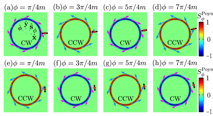
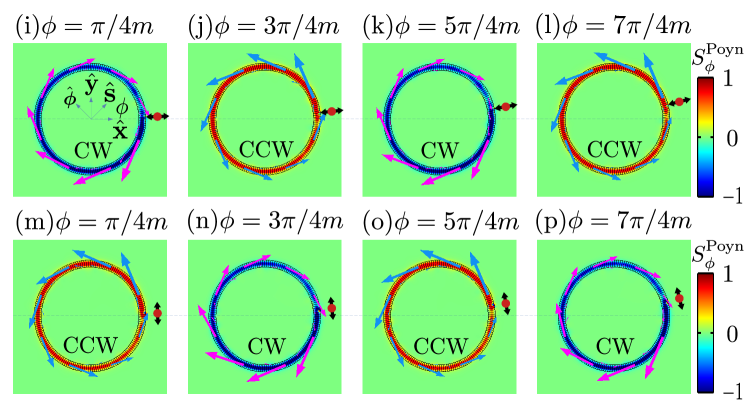
Figure 9: Poynting vectors ($\mathbf{S}^{\rm Poyn}=S_{x}^{\rm Poyn}\hat{\bf x}+S_{y}^{\rm Poyn}\hat{\bf{y}}=S_{s}^{\rm Poyn}\hat{\bf s}+S_{\phi}^{\rm Poyn}\hat{\bm{\phi}}$) from (a-h) QNMs approaches and (i-p) full dipole method for (a-d) ((i-l)) $\hat{\bf s}$ and (e-h) ((m-p)) $\hat{\bm{\phi}}$ dipoles at $\phi=\pi/4m$, $\phi=3\pi/4m$, $\phi=5\pi/4m$, and $\phi=7\pi/4m$ (the radial distance between the dipole and the ring surface is $10\leavevmode\nobreak\$nm ($\delta n_{\rm Re}=\delta n_{\rm Im}=0.001$). The red dot with double black arrows schematically describe the position and polarization of the linear dipoles. The Poynting vectors are labelled as the magenta (for CW direction) and blue (for CCW direction) arrows. The distributions are normalized to $S^{\rm Poyn}_{\phi}$ (for those from full dipole method, they are with arb. units). These power flows are calculated at a example real frequency $\omega=2.50543\times 10^{15}$ (${\rm rad/s}$) (close to QNM resonance). In the ring region, one will find $S^{\rm Poyn}_{\phi}<0$ for CW propagation and $S^{\rm Poyn}_{\phi}>0$ for CCW propagation; the net power flow from QNMs approaches are in excellent agreement with the full dipole simulations.

VI.1 Purcell factors versus frequency for different dipole locations

To confirm the accuracy of our two QNM description for the index-modulated ring resonators, we calculate the Purcell factors analytically from the QNM properties (Eq. (5)) for a $\hat{\bm{\phi}}$ dipole at $\phi=0$ (equal to $\hat{\bf y}$ at $\phi=0$, $\mathbf{d}_{1}$ in Fig. 8 (c)), and compare them with the full dipole method (Eq. (LABEL:Purcellfulldipole)). For all configurations investigated, an excellent agreement is shown as a function of frequency as demonstrated in Fig. 8, where the results for six cases are investigated with the analytical two QNM expansion are studied, including $\delta n_{\rm Im}=0.0005,0.0008,0.001,0.0011,0.0012,0.0015$ while keeping $\delta n_{\rm Re}=0.001$. Their eigenfrequencies are marked in Fig. 8(e). Although there are no material gain regions in these resonators, we also note the appearance of modal negative Purcell factors. This level of agreement is unusual in the sense that the eigenmodes in Ref. Chen et al. (2020) were reported to be completely decoupled, which was used to argue a chiral emission, an effect that is not expected nor obtained for a regular ring resonator. We will connect to the power flow emission below, and show that it is also well explained in terms of the underlying QNMs.

VI.2 Chiral power flow from linearly polarized dipoles

To directly connect with the experimentally measured chirality in Ref. Chen et al., 2020 from linear dipole emitters, here we show chiral power flow using only the QNM propagators in a similar microring with refractive index modulation. We can easily obtain the power flow by computing the scattered fields and the Poynting vector from QNMs and the QNM propagator, and thus the calculations are basically instantaneous.

Once the QNMs are known, the scattered field (in real frequency space) at any point ${\bf r}$ from a dipole at ${\bf r}_{\rm d}$ is simply

$$\mathbf{E}^{\rm scatt}(\mathbf{r},\omega) =\mathbf{G}(\mathbf{r},\mathbf{r}_{\rm d},\omega)\cdot\mathbf{d}$$

$$=[A_{1}(\omega) \tilde{\bf f}_{1}({\bf r})\tilde{\bf f}_{1}({\bf r}_{\rm d})+A_{2}(\omega)\tilde{\bf f}_{2}({\bf r})\tilde{\bf f}_{2}({\bf r}_{\rm d})]\cdot d_{0}{\bf n_{\rm d}},$$ (64)

where ${\bf d}=d_{0}{\bf n}_{\rm d}$, and we will consider both $\hat{\bf s}$ dipoles and $\hat{\bm{\phi}}$ dipoles (i.e., ${\bf n}_{\rm d}=\hat{\bf s}$ or ${\bf n}_{\rm d}=\hat{\bm{\phi}}$). The magnetic scattered field is then

$$\begin{split}\nabla\times\mathbf{E}^{\rm scatt}(\mathbf{r},\omega)&=i\omega\mu_{0}\mathbf{H^{\rm scatt}}(\mathbf{r},\omega)\end{split}$$ (65)

and thus the Poynting vector is simply

$$\begin{split}\mathbf{S}^{\rm Poyn}(\mathbf{r},\omega)&=\frac{1}{2}{\rm Re}[\mathbf{E}^{\rm scatt}(\mathbf{r},\omega)\times\mathbf{H}^{\rm scatt\leavevmode\nobreak\ *}(\mathbf{r},\omega)]\\ &={S}_{x}^{\rm Poyn}(\mathbf{r},\omega)\hat{\bf x}+{S}_{y}^{\rm Poyn}(\mathbf{r},\omega)\hat{\bf y}\\ &={S}_{s}^{\rm Poyn}(\mathbf{r},\omega)\hat{\bf s}+{S}_{\phi}^{\rm Poyn}(\mathbf{r},\omega)\hat{\bm{\phi}},\end{split}$$ (66)

where $S_{\phi}^{\rm Poyn}(\mathbf{r},\omega)$ is the projection along $\hat{\bm{\phi}}$, and one will find $S_{\phi}^{\rm Poyn}(\mathbf{r},\omega)<0$ ($>0$) when it goes along the CW (CCW) direction. Using the QNMs, we stress that we can compute the direction of the power flow and scattered fields analytically, for any dipole position and orientation. This further demonstrates the power of having an analytical expression for the Green function in terms of only QNM properties.

In this section, we focus on the case with $\delta n_{\rm Re}=\delta n_{\rm Im}=0.001$, which is closest to the EP as seen from Fig. 8(e) and Fig. 8(c). Figure 9(a-h) shows the chiral power flow (Eq. (66)) from our QNMs model, for $\hat{\bf s}$ and $\hat{\bm{\phi}}$ dipole at several specific positions, including $\phi=\pi/4m$ (center of two lossy sections, see Fig. 8(c)), $\phi=3\pi/4m$ (center of two lossless sections), $\phi=5\pi/4m$ (center of two lossy sections), and $\phi=7\pi/4m$ (center of two lossless sections) (the radial distance between the dipole and the ring surface is $10\leavevmode\nobreak\$nm). The red dot with a double black arrows in Fig. 9 schematically shows the position and polarization of these linear dipoles (though this is not to scale). Also note that these power flows presented in Fig. 9 are calculated at a example real frequency $\omega=2.50543\times 10^{15}$ (${\rm rad/s}$) (close to QNM resonance), and we stress that the chirality will remain the same in a range around $\omega_{0}\pm 1.5\gamma_{0}$.

The first thing to observe, is that when a linear $\hat{\bf s}$ dipole is placed at $\phi=\pi/4m$ (Fig. 9 (a)), the net power flow ($\mathbf{S}^{\rm Poyn}$, Eq. (66)), indicate by the magenta arrows, goes along the CW direction. The distribution shown is normalized to the projection $S_{\phi}^{\rm Poyn}$. We also find that $S_{\phi}^{\rm Poyn}<0$ in the ring region, which further confirms the net energy flow goes along the CW direction. In addition, the azimuthal period of such phenomenon is $\pi/m$, i.e., when a linear $\hat{\bf s}$ dipole is located at $\phi=\frac{\pi}{4m}+p\frac{\pi}{m}$ (center of the two lossy regions), where $p=0,1,2,...$, the net power will go along the CW direction, such as at $\phi=5\pi/4m$ shown in Fig. 9 (c).

To further justify that our QNM picture is both correct and rigorously accurate for describing this chiral emission, we have confirmed these unusual properties with full dipole calculations shown in Fig. 9 ((i) and (k)). This also supports the experimental findings in Ref. Chen et al., 2020, where they measured CW propagation when putting a linear dipole at $\phi=\pi/4l$ (center of lossy region) (azimuthal mode number $l=1$ in their considered structure, and we are using azimuthal mode number $m=21$ for a similar ring structure). However, our interpretation is drastically different. Instead or arguing a decoupling from the eigenmodes and coupling to a missing dimension, we find that our net chiral power flows are fully explained from the underlying QNMs, which are the correct natural eigenmodes of such resonators.

Moreover, we also find that such unusual properties are not limited to $\hat{\bf s}$ dipoles at $\phi=\frac{\pi}{4m}+p\frac{\pi}{m}$. As shown in Fig. 9(b,d) (QNMs results) and Fig. 9 (j,l) (full dipole results), when a linear $\hat{\bf s}$ dipole is placed at $\phi=\frac{3\pi}{4m}+p\frac{\pi}{m}$ (center of the two lossless sections, where $p=0,1,2,...$), the net power flow is along the CCW direction. In addition, as shown in Fig. 9 (e-h) (QNMs results) and Fig. 9 (m-p) (full dipole results), when a linear $\hat{\bm{\phi}}$ dipole is placed at $\phi=\frac{\pi}{4m}+p\frac{\pi}{m}$ ($\phi=\frac{3\pi}{4m}+p\frac{\pi}{m}$), the net power flow will go along the CCW (CW) direction. Also note, for $\hat{\bf s}$ dipoles at $\phi=n\frac{\pi}{m}$ and $\phi=\frac{2\pi}{4m}+n\frac{\pi}{m}$ (cf. Fig. 8), respectively, the power flow direction will change from CCW to CW and CW to CCW, around resonance, i.e., at resonance, there is no net flow direction. This is also true for $\hat{\bm{\phi}}$ dipoles; for $\hat{\bm{\phi}}$ at $\phi=n\frac{\pi}{m}$ ($\phi=\frac{2\pi}{4m}+n\frac{\pi}{m}$), the power flow direction will change from CW (CCW) to CCW (CW). This gives one an external control to change the directionality by simply changing the frequency.

Note that such chirality behaviour is not found in regular ring resonators (without a refractive modulation) for linear $\hat{\bf s}$ and $\hat{\bm{\phi}}$ dipoles, i.e., no net power flow is obtained. However, by using a circular dipole close to or inside the general ring resonator, chirality will exist, as shown in Ref. Martin-Cano et al., 2019, where positional dependent chirality for right- or left-handed circular dipoles are demonstrated. This is also similar to how one excites unidirectional propagation in photonic crystal waveguides Young et al. (2015); Söllner et al. (2015). However, in all these cases, local symmetry breaking is possible by using a circularly polarized dipole.

VII Conclusions

We have introduced a powerful and highly accurate QNM approach to coupled loss-gain resonators, and have presented a rigorous and intuitive CMT based on the photonic Green function, which allows one to solve the coupled system efficiently with just the bare QNM solutions from the individual resonators. We have also highlighted the failure of using a NM CMT approach when defining the general conditions for finding EPs.

For the SE response of embedded dipoles in these systems, we have carried out detailed calculations for coupled microdisk resonators; as well as finding Lorentzian-like and Lorentzian-suqared like responses at the EP, consistent with other works, we have shown much richer Purcell factor lineshapes near EPs for various designs and spatial dipole positions, showing excellent agreement with QNM CMT and full dipole calculations. In particular, we have shown how the Purcell factors can also be negative, in loss-gain media, even when the hybrid modes are both lossy ($\gamma_{\mu}>0$). This is caused by a breakdown of Fermi’s golden rule which incorrectly assumes that the SE rate is propositional to the (projected) LDOS) Franke et al. (2021). In addition, we also showed how the Green function propagators (related to various experimental observables, such as the emitted spectrum) also take on rich non-Lorentzian features, which depend on the values of the QNM phases.

In addition to the coupled loss and gain resonators, we also investigated EP-like resonances formed from index-modulated ring resonators, where unusual chiral emission from linearly polarized diploes was recently observed Chen et al. (2020). Once again, we showed that the full dipole Purcell factor response is quantitatively well explained in terms of the main two QNMs of this resonator. Moreover, when a linear $\hat{\bf s}$ dipole is located at $\phi=\pi/4m$, the Poynting vectors from QNMs propagators goes along the CW direction, which supports the experimental findings in Ref. Chen et al., 2020 for similar ring resonators. Notably, our explanation is in contrast with the view that the emitter does not couple to the system eigenmodes. In addition, we also showed that such chirality is not limited to $\hat{\bf s}$ dipoles at $\phi=\frac{\pi}{4m}+p\frac{\pi}{m}$, and we also show the opposite chirality for $\hat{\bf s}$ dipoles at $\phi=\frac{3\pi}{4m}+p\frac{\pi}{m}$. There is also similar chirality for linear $\hat{\bm{\phi}}$ dipoles at these positions. We stress, again, that these net power flows can be well explained and interpreted from the two underling QNMs and the corresponding Green function, where the QNM phases play a decisive and fundamental role on the light emission, without having to invoke any unusual interpretation such as a missing dimension (Jordan vector).

Apart from providing a detailed and intuitive formalism for understanding the classical mode properties of these complex coupled resonator systems, our QNM formalism forms the basis for a rigorous quantum optics approach in media with gain and loss, using new approaches with quantized QNMs Franke et al. (2019, 2020a, 2020b), which has already lead to a revision of the usual photonic Fermi’s golden rule for coupled loss and gain resonators Franke et al. (2021), one in which the net Purcell factor is always a positive quantity.

VIII Acknowledgements

We acknowledge funding from Queen’s University, the Canadian Foundation for Innovation, the Natural Sciences and Engineering Research Council of Canada, and CMC Microsystems for the provision of COMSOL Multiphysics. We also acknowledge support from the Alexander von Humboldt Foundation through a Humboldt Research Award. We thank Andreas Knorr for discussions and support, and Thomas Christopoulos for discussions about PML properties in COMSOL.

Appendix A Quasinormal mode (QNM) normalization

There are several general numerical approaches to obtaining normalized QNMs Kristensen et al. (2020), including a dipole excitation technique in complex frequency Bai et al. (2013), PML normalization Sauvan et al. (2013), finite domain normalization with a surface term Muljarov et al. (2010); Kristensen et al. (2015); Muljarov and Langbein (2016), finite-difference time-domain methods Ge and Hughes (2014), and Riesz-projection-based techniques Zschiedrich et al. (2018). In the main text, we use the dipole technique in complex frequency space Bai et al. (2013), and more details are shown in the following subsection A.1. A brief description of two alternative methods is also given in subsections A.2-A.3; numerically, we find all three approaches give the same normalized QNMs for the QNMs used in this work (within numerical precision).

A.1 QNM normalization and numerically exact Green function from a dipole source

As shown in main text, with CMT and the Green function theory, only the bare mode solutions (for a single lossy resonator or gain resonator) are required. We employ an efficient dipole scattering approach to obtain the uncoupled QNMs in complex frequency Bai et al. (2013), where an out-of-plane line current (a point in 2D, red dot in Fig. 1, for a TM mode; it’s a in-plane point dipole for a TE mode) is placed close to the lossy resonator, or the gain resonator, or the index-modulated ring resonators. We can also use this approach for the coupled resonator problem, which we also do to check the accuracy of the analytical CMT for the hybrid modes (see Appendix LABEL:sec:directQNMs).

The scattered field of this dipole at $\mathbf{r}_{0}$ is related to the 2D Green function, from

$$\mathbf{E^{\rm scatt}(\mathbf{r},\omega)}=\mathbf{G}^{\rm 2D}(\mathbf{r},\mathbf{r}_{0},\omega)\cdot\frac{\mathbf{d}^{\rm 2D}}{\epsilon_{0}}.$$ (67)

where the units of the scattered field $\mathbf{E^{\rm scatt}}$, 2D Green function $\mathbf{G}^{\rm 2D}$, and 2D dipole moment $\mathbf{d}^{\rm 2D}$ are, respectively, $\rm V/m$, ${\rm m}^{-2}$, and $\rm C$.

Expanding the 2D Green function with one QNM (dominating in the regime of interest), then

$$\mathbf{G}^{\rm 2D}(\mathbf{r},\mathbf{r}_{0},\omega)=A_{\rm c}(\omega)\tilde{\mathbf{f}}_{\rm c}^{\rm 2D}(\mathbf{r})\tilde{\mathbf{f}}_{\rm c}^{\rm 2D}(\mathbf{r}_{0}),$$ (68)

so that

$$\mathbf{E}^{\rm scatt}(\mathbf{r},\omega)=\frac{1}{\epsilon_{0}}A(\omega)\tilde{\mathbf{f}}_{\rm c}^{\rm 2D}(\mathbf{r})\tilde{\mathbf{f}}_{\rm c}^{\rm 2D}(\mathbf{r}_{0})\cdot\mathbf{d}^{\rm 2D}.$$ (69)

Multiplying Eq. (69) with $\mathbf{d}^{\rm 2D}$ and using $\mathbf{r}=\mathbf{r}_{0}$, then

$$\mathbf{d}^{\rm 2D}\cdot\tilde{\mathbf{f}}^{\rm 2D}_{\rm c}(\mathbf{r}_{0})=\sqrt{\frac{\epsilon_{0}\mathbf{d}^{\rm 2D}\cdot\mathbf{E}^{\rm scatt}(\mathbf{r}_{0},\omega)}{A(\omega)}}.$$ (70)

Substituting this back to Eq. (69), we obtain the 2D normalized QNM field as a function of space

$$\begin{split}\tilde{\mathbf{f}}^{\rm 2D}_{\rm c}(\mathbf{r})&=\sqrt{\frac{\epsilon_{0}}{A(\omega)\mathbf{d}^{\rm 2D}\cdot\mathbf{E}^{\rm scatt}(\mathbf{r}_{0},\omega)}}\mathbf{E}^{\rm scatt}(\mathbf{r},\omega),\\ &=\sqrt{\frac{2\epsilon_{0}(\tilde{\omega}_{\rm c}-\omega)}{\omega\mathbf{d}^{\rm 2D}\cdot\mathbf{E}^{\rm scatt}(\mathbf{r}_{0},\omega)}}\mathbf{E}^{\rm scatt}(\mathbf{r},\omega).\end{split}$$ (71)

The above QNM simulations are performed in the commercial COMSOL software COMSOL Inc. , where the frequency in Eq. (71) is set as $\omega=(1-10^{-7})\times\tilde{\omega}_{\rm c}$ (or $(1-10^{-6})\times\tilde{\omega}_{\rm c}$, $(1-10^{-8})\times\tilde{\omega}_{\rm c}$, adjust with the quality factors), very close to the pole frequency. The computational domain (including PMLs) is around $804\sim 814$ $\mu$m² (various gap distance for microdisk resonators; for microring resonators, it’s around $72$ $\mu$m²), where the maximum mesh element sizes are $0.1$ nm, $40$ nm and $75$ nm at the dipole point, inside and outside the 2D microdisks. To minimize boundary reflections, we used $15$ layers to form the PMLs with a total thickness of $1.5$ $\mu$m, which was found to be well converged numerically.

In addition, once the normalized QNMs are available, the corresponding effective mode area (with units ${\rm m}^{2}$), which is a function of position, is obtained from

$$A_{\rm c}^{\rm eff}(\mathbf{r}_{0})=\frac{1}{\epsilon(\mathbf{r}_{0}){\rm Re}[{\bf f}^{2}_{\rm c,2D}(\mathbf{r}_{0})]}.$$ (72)

The decay rates for 2D dipoles are as follows:

$$\begin{split}\Gamma^{\rm 2D}(\mathbf{r}_{0},\omega)&=\frac{2}{\hbar\epsilon_{0}}\mathbf{d}^{\rm 2D}\cdot{\rm Im}\{\mathbf{G}^{\rm 2D}(\mathbf{r}_{0},\mathbf{r}_{0},\omega)\}\cdot\mathbf{d}^{\rm 2D},\\ \Gamma^{\rm 2D}_{0}(\mathbf{r}_{0},\omega)&=\frac{2}{\hbar\epsilon_{0}}\mathbf{d}^{\rm 2D}\cdot{\rm Im}\{\mathbf{G}^{\rm 2D}_{\rm B}(\mathbf{r}_{0},\mathbf{r}_{0},\omega)\}\cdot\mathbf{d}^{\rm 2D},\end{split}$$ (73)

where ${\rm Im}\{\mathbf{G}_{\rm B}(\mathbf{r}_{0},\mathbf{r}_{0},\omega)\}={\omega^{2}}/{4c^{2}}$ (${\omega^{2}}/{8c^{2}}$) for a 2D TM (TE) dipole, and the units of $\Gamma^{\rm 2D}$ is $1/({\rm s}\cdot{\rm m})$.

The corresponding Purcell factor is simply Anger et al. (2006); Kristensen and Hughes (2014)

$$\begin{split}&F^{\rm 2D}(\mathbf{r}_{0},\omega)=1+\frac{\Gamma^{\rm 2D}(\mathbf{r}_{0},\omega)}{\Gamma^{\rm 2D}_{0}(\mathbf{r}_{0},\omega)},\end{split}$$ (74)

and similar expressions are obtained for 3D systems.

A.2 Perfectly matched later (PML) normalization

The PML normalization Sauvan et al. (2013); Vial et al. (2014); Lalanne et al. (2018) approach is another alternative way to get the normalized QNMs, which is given via (for dispersive and nonmagnetic materials)

$$\begin{split}\braket{\braket{\tilde{\mathbf{f}}_{\mu}(\mathbf{r})}{\tilde{\mathbf{f}}_{\mu}(\mathbf{r})}}{=}\frac{1}{2}\int_{V-V_{\rm PML}}\bigg{[}\frac{\partial(\omega\epsilon(\mathbf{r},\omega))}{\partial\omega}\Big{|}_{\tilde{\omega}_{\mu}}\tilde{\mathbf{f}}_{\mu}(\mathbf{r})\cdot\tilde{\mathbf{f}}_{\mu}(\mathbf{r})\\ +\epsilon(\mathbf{r},\tilde{\omega}_{\mu})\tilde{\mathbf{f}}_{\mu}(\mathbf{r})\cdot\tilde{\mathbf{f}}_{\mu}(\mathbf{r})\bigg{]}dV\\ +\frac{1}{2\epsilon_{0}}\int_{V_{\rm PML}}\bigg{[}\epsilon_{0}\frac{\partial(\omega\epsilon_{\rm PML}(\mathbf{r},\omega))}{\partial\omega}\Big{|}_{\tilde{\omega}_{\mu}}\tilde{\mathbf{f}}_{\mu}(\mathbf{r})\cdot\tilde{\mathbf{f}}_{\mu}(\mathbf{r})\\ -\mu_{0}\frac{\partial(\omega\mu_{\rm PML}(\mathbf{r},\omega))}{\partial\omega}\Big{|}_{\tilde{\omega}_{\mu}}\tilde{\mathbf{h}}_{\mu}(\mathbf{r})\cdot\tilde{\mathbf{h}}_{\mu}(\mathbf{r})\bigg{]}dV=1,\end{split}$$ (75)

where $\tilde{\mathbf{h}}_{\mu}(\mathbf{r})$ is the magnetic field of QNM, $V$ is the whole simulation region, and $V_{\rm PML}$ denotes the PML region. Outside the PML region, then the fields are zero.

For a nondispersive and nonmagnetic material,

$$\begin{split}\braket{\braket{\tilde{\mathbf{f}}_{\mu}(\mathbf{r})}{\tilde{\mathbf{f}}_{\mu}(\mathbf{r})}}{=}\int_{V-V_{\rm PML}}\bigg{[}\epsilon(\mathbf{r})\tilde{\mathbf{f}}_{\mu}(\mathbf{r})\cdot\tilde{\mathbf{f}}_{\mu}(\mathbf{r})\bigg{]}dV\\ +\frac{1}{2\epsilon_{0}}\int_{V_{\rm PML}}\bigg{[}\epsilon_{0}\frac{\partial(\omega\epsilon_{\rm PML}(\mathbf{r},\omega))}{\partial\omega}\Big{|}_{\tilde{\omega}_{\mu}}\tilde{\mathbf{f}}_{\mu}(\mathbf{r})\cdot\tilde{\mathbf{f}}_{\mu}(\mathbf{r})\\ -\mu_{0}\frac{\partial(\omega\mu_{\rm PML}(\mathbf{r},\omega))}{\partial\omega}\Big{|}_{\tilde{\omega}_{\mu}}\tilde{\mathbf{h}}_{\mu}(\mathbf{r})\cdot\tilde{\mathbf{h}}_{\mu}(\mathbf{r})\bigg{]}dV=1,\end{split}$$ (76)

and extra care is needed for the PML region (second term in Eq. (76)), though this contribution can be very small for certain problems and geometries. In general, there are several kinds of transformation performed in PMLs to minimize boundary reflections. The first one is using special permittivity $\epsilon_{\rm PML}(\mathbf{r},\omega)$ and permeability $\mu_{\rm PML}(\mathbf{r},\omega)$ values, which is not always available with some commercial software Lalanne et al. (2018). A second approach uses a coordinate transformation, which is what we used here, with the built-in stretched-coordinate PML of COMSOL, where the coordinates are transferred from real space to the complex plane Berenger (1994).

To verify that the dipole normalization technique and PML normalization are consistent with each other, we performed the norm calculation (Eq. (76)) using the QNM fields from the dipole technique. We obtained $\braket{\braket{\tilde{\mathbf{f}}^{\rm L}(\mathbf{r})}{\tilde{\mathbf{f}}^{\rm L}(\mathbf{r})}}{=}1.0004-0.0011i\sim 1$ for the QNM of interest from the single lossy WGM resonator with $n_{\rm loss}=2+10^{-5}i$, and $\braket{\braket{\tilde{\mathbf{f}}^{\rm G}(\mathbf{r})}{\tilde{\mathbf{f}}^{\rm G}(\mathbf{r})}}{=}0.9991+0.0006i\sim 1$ for the QNM of interest from single gain WGM resonator with $n_{\rm gain}=2-5\times 10^{-6}i$. However, note, that for our chosen PML geometry and resonator, the contribution from the PML is practically negligible for this problem of interest (high $Q$ resonance).

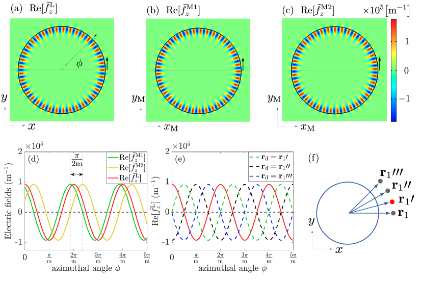
Figure 10: Spatial profile of the degenerate QNMs for a single lossy resonator. (a) QNM obtained with a general QNM approach (Eq. (71)) (it is the same as in Fig. 4 (a)), where only one of the degenerate standing wave modes is excited, which is with a $cos(m\phi)$ dependence, considering $\phi=0$ at the positive $x$-axis. (b-c) Normalized (Eq. (LABEL:eq:pmlnorm_M1M2)) degenerate modes $1$ and $2$ from the eigenfrequency solver using COMSOL, where the boundary condition is with PML. The horizontal dashed lines in (a), (b), and (c) labeled the $x$-axis with their own coordinates. (d) The fields at the disk edge along vertical arrow (in (a), (b), and (c)). (e) Same as in (a) but when the dipole position is moved to a different position, as shown in (f).

A.3 Finite-domain normalization with a surface term

A third way to normalize QNMs is through a finite domain normalization with an outgoing surface term Muljarov et al. (2010); Muljarov and Langbein (2016); Kristensen et al. (2015, 2020), is given by

$$\braket{\braket{\tilde{\mathbf{f}}_{\mu}(\mathbf{r})}{\tilde{\mathbf{f}}_{\mu}(\mathbf{r})}}{$&}=\frac{1}{2\epsilon_{0}}\int_{V}\bigg{[}\epsilon_{0}\frac{\partial(\omega\epsilon(\mathbf{r},\omega))}{\partial\omega}\Big{|}_{\tilde{\omega}_{\mu}}\tilde{\mathbf{f}}_{\mu}(\mathbf{r})\cdot\tilde{\mathbf{f}}_{\mu}(\mathbf{r}$$

$$-\mu_{0}\tilde{\mathbf{h}}_{\mu}(\mathbf{r})\cdot\tilde{\mathbf{h}}_{\mu}(\mathbf{r})\bigg{]}dV$$

$$+\frac{i}{2\epsilon_{0}\tilde{\omega}_{\mu}}\int_{\partial V}\bigg{[}\big{(}r\partial r\tilde{\mathbf{f}}_{\mu}(\mathbf{r})\big{)}\mathbf{\times}\tilde{\mathbf{h}}_{\mu}(\mathbf{r})$$

$$-\tilde{\mathbf{f}}_{\mu}(\mathbf{r})\mathbf{\times}\big{(}r\partial{r}\tilde{\mathbf{h}}_{\mu}(\mathbf{r})\big{)}\bigg{]}\cdot\hat{\mathbf{n}}dA=1,$$ (77)

or

Appendix F Additional loss-gain resonator examples with different gain coefficients

Finally, we also show the Purcell factors for two additional loss-gain resonator examples, for different amounts of gain. The refractive index for the lossy resonator is fixed at $n_{\rm loss}=2+10^{-5}i$, as in the main text. When $n_{\rm gain}=2-6\times 10^{-6}i$, the Purcell factors with a gap distance $d_{\rm gap}=1145\leavevmode\nobreak\$nm (close to the lossy EP) for a dipole at $\mathbf{r}_{1}$ ($10$ nm away from the lossy cavity) are shown in Fig. LABEL:fig6(a), which show very good agreement with the full dipole method. Again, we see that negative Purcell factors are obtained over a wide frequency range. The separate contributions from $\tilde{\mathbf{f}}^{+}$ and $\tilde{\mathbf{f}}^{-}$ are also given. For better comparison, the Purcell factors with single lossy cavity are shown as an orange dashed curve (the dipole is at $\mathbf{r}_{1}$), which is net positive and multiplied by $30$ for clarity.

Similarly, the corresponding results for the case with $n_{\rm gain}=2-7\times 10^{-6}i$ are shown in Fig. LABEL:fig6(b), where the gap distance is $d_{\rm gap}=1133\leavevmode\nobreak\$nm. Excellent agreement with full dipole results are also obtained. The absolute values of the negative Purcell factors increase here mainly because it is closer to the EP and the gap distance is smaller.

References

- Raabe and Welsch (2008) C. Raabe and D.-G. Welsch, “QED in arbitrary linear media: Amplifying media,” The European Physical Journal Special Topics 160, 371–381 (2008).
- Søndergaard and Tromborg (2001) T. Søndergaard and B. Tromborg, “General theory for spontaneous emission in active dielectric microstructures: Example of a fiber amplifier,” Phys. Rev. A 64, 033812 (2001).
- Bender and Boettcher (1998) Carl M. Bender and Stefan Boettcher, “Real spectra in non-hermitian hamiltonians having symmetry,” Phys. Rev. Lett. 80, 5243–5246 (1998).
- Bender et al. (1999) Carl M Bender, Stefan Boettcher, and Peter N Meisinger, “PT-symmetric quantum mechanics,” J. Math. Phys. 40, 29 (1999).
- Lévai and Znojil (2000) Géza Lévai and Miloslav Znojil, “Systematic search for -symmetric potentials with real energy spectra,” J. Phys. A 33, 7165–7189 (2000).
- Bender et al. (2002a) Carl M Bender, M V Berry, and Aikaterini Mandilara, “Generalized PT symmetry and real spectra,” J. Phys. A: Math. Gen. 35, L467–L471 (2002a).
- Bender et al. (2002b) Carl M. Bender, Dorje C. Brody, and Hugh F. Jones, “Complex extension of quantum mechanics,” Phys. Rev. Lett. 89, 270401 (2002b).
- Mostafazadeh (2002) Ali Mostafazadeh, “Pseudo-hermiticity versus PT symmetry: The necessary condition for the reality of the spectrum of a non-hermitian hamiltonian,” J. Math. Phys. 43, 205–214 (2002).
- Bender et al. (2003) Carl M. Bender, Dorje C. Brody, and Hugh F. Jones, “Must a hamiltonian be hermitian?” American Journal of Physics 71, 1095–1102 (2003).
- Bender (2007) Carl M Bender, “Making sense of non-hermitian hamiltonians,” Rep. Prog. Phys. 70, 947–1018 (2007).
- El-Ganainy et al. (2007) R. El-Ganainy, K. G. Makris, D. N. Christodoulides, and Ziad H. Musslimani, “Theory of coupled optical PT-symmetric structures,” Opt. Lett. 32, 2632 (2007).
- Makris et al. (2008) K. G. Makris, R. El-Ganainy, D. N. Christodoulides, and Z. H. Musslimani, “Beam dynamics in symmetric optical lattices,” Phys. Rev. Lett. 100, 103904 (2008).
- Klaiman et al. (2008) Shachar Klaiman, Uwe Günther, and Nimrod Moiseyev, “Visualization of branch points in -symmetric waveguides,” Phys. Rev. Lett. 101, 080402 (2008).
- Guo et al. (2009) A. Guo, G. J. Salamo, D. Duchesne, R. Morandotti, M. Volatier-Ravat, V. Aimez, G. A. Siviloglou, and D. N. Christodoulides, “Observation of -symmetry breaking in complex optical potentials,” Phys. Rev. Lett. 103, 093902 (2009).
- Longhi (2009) S. Longhi, “Bloch oscillations in complex crystals with symmetry,” Phys. Rev. Lett. 103, 123601 (2009).
- Mostafazadeh (2009) Ali Mostafazadeh, “Spectral singularities of complex scattering potentials and infinite reflection and transmission coefficients at real energies,” Phys. Rev. Lett. 102, 220402 (2009).
- Rüter et al. (2010) Christian E. Rüter, Konstantinos G. Makris, Ramy El-Ganainy, Demetrios N. Christodoulides, Mordechai Segev, and Detlef Kip, “Observation of parity–time symmetry in optics,” Nature Phys. 6, 192–195 (2010).
- Kottos (2010) Tsampikos Kottos, “Broken symmetry makes light work,” Nature Phys. 6, 166–167 (2010).
- Longhi (2010a) Stefano Longhi, “Optical realization of relativistic non-hermitian quantum mechanics,” Phys. Rev. Lett. 105, 013903 (2010a).
- Benisty et al. (2015) Henri Benisty, Anatole Lupu, and Aloyse Degiron, “Transverse periodic symmetry for modal demultiplexing in optical waveguides,” Phys. Rev. A 91, 053825 (2015).
- Konotop et al. (2016) Vladimir V. Konotop, Jianke Yang, and Dmitry A. Zezyulin, “Nonlinear waves in PT -symmetric systems,” Rev. Mod. Phys. 88, 035002 (2016).
- Feng et al. (2017) Liang Feng, Ramy El-Ganainy, and Li Ge, “Non-hermitian photonics based on parity-time symmetry,” Nature Photon. 11, 752–762 (2017).
- Longhi (2017) Stefano Longhi, “Parity-time symmetry meets photonics: A new twist in non-hermitian optics,” EPL 120, 64001 (2017).
- Lupu et al. (2017) Anatole Lupu, Vladimir V. Konotop, and Henri Benisty, “Optimal -symmetric switch features exceptional point,” Scientific Reports 7, 13299 (2017).
- El-Ganainy et al. (2018) Ramy El-Ganainy, Konstantinos G. Makris, Mercedeh Khajavikhan, Ziad H. Musslimani, Stefan Rotter, and Demetrios N. Christodoulides, “Non-hermitian physics and PT symmetry,” Nature Phys. 14, 11–19 (2018).
- Jin (2018) L. Jin, “Parity-time-symmetric coupled asymmetric dimers,” Physical Review A 97, 012121 (2018).
- Morozko et al. (2020) Fyodor Morozko, Andrey Novitsky, and Alina Karabchevsky, “Modal purcell factor in $\mathcal{PT}$-symmetric waveguides,” Physical Review B 102, 155303 (2020), publisher: American Physical Society.
- Berry (2004) M.V. Berry, “Physics of nonhermitian degeneracies,” Czechoslovak Journal of Physics 54, 1039–1047 (2004).
- Heiss (2004) W D Heiss, “Exceptional points of non-hermitian operators,” J. Phys. A: Math. Gen. 37, 2455–2464 (2004).
- Heiss (2012) W D Heiss, “The physics of exceptional points,” J. Phys. A: Math. Theor. 45, 444016 (2012).
- Ding et al. (2016) Kun Ding, Guancong Ma, Meng Xiao, Z. Q. Zhang, and C. T. Chan, “Emergence, coalescence, and topological properties of multiple exceptional points and their experimental realization,” Phys. Rev. X 6, 021007 (2016).
- Miri and Alù (2019) Mohammad-Ali Miri and Andrea Alù, “Exceptional points in optics and photonics,” Science 363, eaar7709 (2019).
- Chen et al. (2019) Chong Chen, Liang Jin, and Ren-Bao Liu, “Sensitivity of parameter estimation near the exceptional point of a non-hermitian system,” New Journal of Physics 21, 083002 (2019).
- Jin et al. (2020) L. Jin, H. C. Wu, Bo-Bo Wei, and Z. Song, “Hybrid exceptional point created from type-III dirac point,” Physical Review B 101, 045130 (2020).
- Lin et al. (2011) Zin Lin, Hamidreza Ramezani, Toni Eichelkraut, Tsampikos Kottos, Hui Cao, and Demetrios N. Christodoulides, “Unidirectional invisibility induced by PT-symmetric periodic structures,” Phys. Rev. Lett. 106, 213901 (2011).
- Feng et al. (2013) Liang Feng, Ye-Long Xu, William S. Fegadolli, Ming-Hui Lu, José E. B. Oliveira, Vilson R. Almeida, Yan-Feng Chen, and Axel Scherer, “Experimental demonstration of a unidirectional reflectionless parity-time metamaterial at optical frequencies,” Nature Mater. 12, 108–113 (2013).
- Peng et al. (2014a) Bo Peng, Şahin Kaya Özdemir, Fuchuan Lei, Faraz Monifi, Mariagiovanna Gianfreda, Gui Lu Long, Shanhui Fan, Franco Nori, Carl M. Bender, and Lan Yang, “Parity–time-symmetric whispering-gallery microcavities,” Nature Physics 10, 394–398 (2014a).
- Chang et al. (2014) Long Chang, Xiaoshun Jiang, Shiyue Hua, Chao Yang, Jianming Wen, Liang Jiang, Guanyu Li, Guanzhong Wang, and Min Xiao, “Parity-time symmetry and variable optical isolation in active-passive-coupled microresonators,” Nature Photon. 8, 524–529 (2014).
- Jin and Song (2018) L. Jin and Z. Song, “Incident direction independent wave propagation and unidirectional lasing,” Physical Review Letters 121, 073901 (2018).
- Zyablovsky et al. (2014) A. A. Zyablovsky, A. P. Vinogradov, A. A. Pukhov, A. V. Dorofeenko, and A. A. Lisyansky, “PT-symmetry in optics,” Phys.-Usp. 57, 1063 (2014).
- Doppler et al. (2016) Jörg Doppler, Alexei A. Mailybaev, Julian Böhm, Ulrich Kuhl, Adrian Girschik, Florian Libisch, Thomas J. Milburn, Peter Rabl, Nimrod Moiseyev, and Stefan Rotter, “Dynamically encircling an exceptional point for asymmetric mode switching,” Nature 537, 76–79 (2016).
- Xu et al. (2016) H. Xu, D. Mason, Luyao Jiang, and J. G. E. Harris, “Topological energy transfer in an optomechanical system with exceptional points,” Nature 537, 80–83 (2016).
- Heiss (2016) Dieter Heiss, “Circling exceptional points,” Nature Phys. 12, 823–824 (2016).
- Chen et al. (2017) Weijian Chen, Şahin Kaya Özdemir, Guangming Zhao, Jan Wiersig, and Lan Yang, “Exceptional points enhance sensing in an optical microcavity,” Nature 548, 192–196 (2017).
- Chen et al. (2018) Weijian Chen, Jing Zhang, Bo Peng, Şahin Kaya Özdemir, Xudong Fan, and Lan Yang, “Parity-time-symmetric whispering-gallery mode nanoparticle sensor [invited],” Photonics Research 6, A23–A30 (2018).
- Longhi (2010b) Stefano Longhi, “PT-symmetric laser absorber,” Phys. Rev. A 82, 031801 (2010b).
- Chong et al. (2011) Y. D. Chong, Li Ge, and A. Douglas Stone, “PT-symmetry breaking and laser-absorber modes in optical scattering systems,” Phys. Rev. Lett. 106, 093902 (2011).
- Sun et al. (2014) Yong Sun, Wei Tan, Hong-qiang Li, Jensen Li, and Hong Chen, “Experimental demonstration of a coherent perfect absorber with PT phase transition,” Phys. Rev. Lett. 112, 143903 (2014).
- Jin et al. (2016) L. Jin, P. Wang, and Z. Song, “Unidirectional perfect absorber,” Scientific Reports 6, 32919 (2016).
- Brandstetter et al. (2014) M. Brandstetter, M. Liertzer, C. Deutsch, P. Klang, J. Schöberl, H. E. Türeci, G. Strasser, K. Unterrainer, and S. Rotter, “Reversing the pump dependence of a laser at an exceptional point,” Nat Commun. 5, 4034 (2014).
- Feng et al. (2014) L. Feng, Z. J. Wong, R.-M. Ma, Y. Wang, and X. Zhang, “Single-mode laser by parity-time symmetry breaking,” Science 346, 972–975 (2014).
- Hodaei et al. (2014) H. Hodaei, M.-A. Miri, M. Heinrich, D. N. Christodoulides, and M. Khajavikhan, “Parity-time-symmetric microring lasers,” Science 346, 975–978 (2014).
- Peng et al. (2014b) B. Peng, Ş. K. Özdemir, S. Rotter, H. Yilmaz, M. Liertzer, F. Monifi, C. M. Bender, F. Nori, and L. Yang, “Loss-induced suppression and revival of lasing,” Science 346, 328–332 (2014b).
- Haus and Huang (1991) H.A. Haus and W. Huang, “Coupled-mode theory,” Proceedings of the IEEE 79, 1505–1518 (1991).
- Fan et al. (2003) Shanhui Fan, Wonjoo Suh, and J. D. Joannopoulos, “Temporal coupled-mode theory for the fano resonance in optical resonators,” J. Opt. Soc. Am. A 20, 569 (2003).
- Artar et al. (2011) Alp Artar, Ahmet Ali Yanik, and Hatice Altug, “Directional double Fano resonances in plasmonic hetero-oligomers,” Nano Letters 11, 3694–3700 (2011).
- Yang et al. (2019) Ruisheng Yang, Quanhong Fu, Yuancheng Fan, Weiqi Cai, Kepeng Qiu, Weihong Zhang, and Fuli Zhang, “Active control of EIT-like response in a symmetry-broken metasurface with orthogonal electric dipolar resonators,” Photonics Research 7, 955 (2019).
- Park et al. (2020) Jun-Hee Park, Abdoulaye Ndao, Wei Cai, Liyi Hsu, Ashok Kodigala, Thomas Lepetit, Yu-Hwa Lo, and Boubacar Kanté, “Symmetry-breaking-induced plasmonic exceptional points and nanoscale sensing,” Nature Physics 16, 462–468 (2020).
- Lai et al. (1990) H. M. Lai, P. T. Leung, K. Young, P. W. Barber, and S. C. Hill, “Time-independent perturbation for leaking electromagnetic modes in open systems with application to resonances in microdroplets,” Phys. Rev. A 41, 5187–5198 (1990).
- Leung et al. (1994a) P. T. Leung, S. Y. Liu, and K. Young, “Completeness and orthogonality of quasinormal modes in leaky optical cavities,” Physical Review A 49, 3057–3067 (1994a).
- Leung et al. (1994b) P. T. Leung, S. Y. Liu, S. S. Tong, and K. Young, “Time-independent perturbation theory for quasinormal modes in leaky optical cavities,” Physical Review A 49, 3068–3073 (1994b).
- Leung and Pang (1996) P. T. Leung and K. M. Pang, “Completeness and time-independent perturbation of morphology-dependent resonances in dielectric spheres,” JOSAB 13, 805–817 (1996).
- Lee et al. (1999) K. M. Lee, P. T. Leung, and K. M. Pang, “Dyadic formulation of morphology-dependent resonances. i. completeness relation,” JOSAB 16, 1409–1417 (1999).
- Kristensen et al. (2012) P. T. Kristensen, C. Van Vlack, and S. Hughes, “Generalized effective mode volume for leaky optical cavities,” Optics Letters 37, 1649 (2012).
- Sauvan et al. (2013) C. Sauvan, J. P. Hugonin, I. S. Maksymov, and P. Lalanne, “Theory of the Spontaneous Optical Emission of Nanosize Photonic and Plasmon Resonators,” Physical Review Letters 110, 237401 (2013).
- Kristensen and Hughes (2014) Philip Trøst Kristensen and Stephen Hughes, “Modes and Mode Volumes of Leaky Optical Cavities and Plasmonic Nanoresonators,” ACS Photonics 1, 2–10 (2014).
- Bai et al. (2013) Q. Bai, M. Perrin, C. Sauvan, J.-P. Hugonin, and P. Lalanne, “Efficient and intuitive method for the analysis of light scattering by a resonant nanostructure,” Optics Express 21, 27371–27382 (2013).
- Zschiedrich et al. (2018) Lin Zschiedrich, Felix Binkowski, Niko Nikolay, Oliver Benson, Günter Kewes, and Sven Burger, “Riesz-projection-based theory of light-matter interaction in dispersive nanoresonators,” Phys. Rev. A 98, 043806 (2018).
- Alpeggiani et al. (2017) Filippo Alpeggiani, Nikhil Parappurath, Ewold Verhagen, and L. Kuipers, “Quasinormal-mode expansion of the scattering matrix,” Phys. Rev. X 7, 021035 (2017).
- Lalanne et al. (2018) Philippe Lalanne, Wei Yan, Kevin Vynck, Christophe Sauvan, and Jean-Paul Hugonin, “Light interaction with photonic and plasmonic resonances,” Laser & Photonics Reviews 12, 1700113 (2018).
- Kristensen et al. (2020) Philip Trøst Kristensen, Kathrin Herrmann, Francesco Intravaia, and Kurt Busch, “Modeling electromagnetic resonators using quasinormal modes,” Advances in Optics and Photonics 12, 612 (2020).
- Muljarov et al. (2010) E. A. Muljarov, W. Langbein, and R. Zimmermann, “Brillouin-wigner perturbation theory in open electromagnetic systems,” EPL 92, 50010 (2010).
- Muljarov and Langbein (2016) E. A. Muljarov and W. Langbein, “Exact mode volume and purcell factor of open optical systems,” Physical Review B 94, 235438 (2016).
- Franke et al. (2019) Sebastian Franke, Stephen Hughes, Mohsen Kamandar Dezfouli, Philip Trøst Kristensen, Kurt Busch, Andreas Knorr, and Marten Richter, “Quantization of quasinormal modes for open cavities and plasmonic cavity quantum electrodynamics,” Phys. Rev. Lett. 122, 213901 (2019).
- Franke et al. (2020a) Sebastian Franke, Juanjuan Ren, Stephen Hughes, and Marten Richter, “Fluctuation-dissipation theorem and fundamental photon commutation relations in lossy nanostructures using quasinormal modes,” Phys. Rev. Research 2, 033332 (2020a).
- Franke et al. (2020b) Sebastian Franke, Marten Richter, Juanjuan Ren, Andreas Knorr, and Stephen Hughes, “Quantized quasinormal-mode description of nonlinear cavity-QED effects from coupled resonators with a fano-like resonance,” Phys. Rev. Research 2, 033456 (2020b).
- Vial and Hao (2016) Benjamin Vial and Yang Hao, “A coupling model for quasi-normal modes of photonic resonators,” J. Opt. 18, 115004 (2016).
- Kristensen et al. (2017) Philip Trøst Kristensen, Jakob Rosenkrantz de Lasson, Mikkel Heuck, Niels Gregersen, and Jesper Mørk, “On the theory of coupled modes in optical cavity-waveguide structures,” Journal of Lightwave Technology 35, 4247–4259 (2017).
- Cognée (2020) Kévin G. Cognée, Hybridization of open photonic resonators, PhD dissertation, University of Amsterdam (2020).
- Tao et al. (2020) Can Tao, Junda Zhu, Ying Zhong, and Haitao Liu, “Coupling theory of quasinormal modes for lossy and dispersive plasmonic nanoresonators,” Physical Review B 102, 045430 (2020).
- Chen et al. (2020) Hua-Zhou Chen, Tuo Liu, Hong-Yi Luan, Rong-Juan Liu, Xing-Yuan Wang, Xue-Feng Zhu, Yuan-Bo Li, Zhong-Ming Gu, Shan-Jun Liang, He Gao, Ling Lu, Li Ge, Shuang Zhang, Jie Zhu, and Ren-Min Ma, “Revealing the missing dimension at an exceptional point,” Nature Physics 16, 571–578 (2020).
- Yoo et al. (2011) Gwangsu Yoo, H.-S. Sim, and Henning Schomerus, “Quantum noise and mode nonorthogonality in non-hermitian -symmetric optical resonators,” Phys. Rev. A 84, 063833 (2011).
- Pick et al. (2017a) Adi Pick, Bo Zhen, Owen D. Miller, Chia W. Hsu, Felipe Hernandez, Alejandro W. Rodriguez, Marin Soljačić, and Steven G. Johnson, “General theory of spontaneous emission near exceptional points,” Optics Express 25, 12325 (2017a).
- Khanbekyan and Wiersig (2020) M. Khanbekyan and J. Wiersig, “Decay suppression of spontaneous emission of a single emitter in a high- cavity at exceptional points,” Phys. Rev. Research 2, 023375 (2020).
- Franke et al. (2021) Sebastian Franke, Juanjuan Ren, Marten Richter, Andreas Knorr, and Stephen Hughes, “Fermi’s golden rule for spontaneous emission in absorptive and amplifying media,” (2021), arXiv:2102.13015 .
- Kristensen et al. (2015) Philip Trøst Kristensen, Rong-Chun Ge, and Stephen Hughes, “Normalization of quasinormal modes in leaky optical cavities and plasmonic resonators,” Phys. Rev. A 92, 053810 (2015).
- Ge et al. (2014) Rong-Chun Ge, Philip Trøst Kristensen, Jeff F Young, and Stephen Hughes, “Quasinormal mode approach to modelling light-emission and propagation in nanoplasmonics,” New Journal of Physics 16, 113048 (2014).
- Anger et al. (2006) Pascal Anger, Palash Bharadwaj, and Lukas Novotny, “Enhancement and quenching of single-molecule fluorescence,” Phys. Rev. Lett. 96, 113002 (2006).
- Ge and Hughes (2014) Rong-Chun Ge and S. Hughes, “Design of an efficient single photon source from a metallic nanorod dimer: a quasi-normal mode finite-difference time-domain approach,” Opt. Lett. 39, 4235 (2014).
- Cowan and Young (2003) A. R. Cowan and Jeff F. Young, “Optical bistability involving photonic crystal microcavities and fano line shapes,” Phys. Rev. E 68, 046606 (2003).
- Ren et al. (2020) Juanjuan Ren, Sebastian Franke, Andreas Knorr, Marten Richter, and Stephen Hughes, “Near-field to far-field transformations of optical quasinormal modes and efficient calculation of quantized quasinormal modes for open cavities and plasmonic resonators,” Phys. Rev. B 101, 205402 (2020).
- Peng et al. (2016) Bo Peng, Şahin Kaya Özdemir, Matthias Liertzer, Weijian Chen, Johannes Kramer, Huzeyfe Yılmaz, Jan Wiersig, Stefan Rotter, and Lan Yang, “Chiral modes and directional lasing at exceptional points,” Proceedings of the National Academy of Sciences 113, 6845–6850 (2016).
- Sunada (2018) Satoshi Sunada, “Enhanced response of non-hermitian photonic systems near exceptional points,” Physical Review A 97, 043804 (2018).
- Lin et al. (2016) Zin Lin, Adi Pick, Marko Lončar, and Alejandro W. Rodriguez, “Enhanced spontaneous emission at third-order dirac exceptional points in inverse-designed photonic crystals,” Physical Review Letters 117, 107402 (2016).
- Pick et al. (2017b) Adi Pick, Zin Lin, Weiliang Jin, and Alejandro W. Rodriguez, “Enhanced nonlinear frequency conversion and Purcell enhancement at exceptional points,” Physical Review B 96, 224303 (2017b).
- de Lasson et al. (2015) Jakob Rosenkrantz de Lasson, Philip Trøst Kristensen, Jesper Mørk, and Niels Gregersen, “Semianalytical quasi-normal mode theory for the local density of states in coupled photonic crystal cavity–waveguide structures,” Optics Letters 40, 5790 (2015).
- Kamandar Dezfouli et al. (2017) Mohsen Kamandar Dezfouli, Reuven Gordon, and Stephen Hughes, “Modal theory of modified spontaneous emission of a quantum emitter in a hybrid plasmonic photonic-crystal cavity system,” Phys. Rev. A 95, 013846 (2017).
- El-Sayed and Hughes (2020) Al-Waleed El-Sayed and Stephen Hughes, “Quasinormal-mode theory of elastic Purcell factors and Fano resonances of optomechanical beams,” Physical Review Research 2, 043290 (2020).
- Righini et al. (2011) G. C. Righini, Y. Dumeige, P. Féron, M. Ferrari, G. Nunzi Conti, D. Ristic, and S. Soria, “Whispering gallery mode microresonators: Fundamentals and applications,” La Rivista del Nuovo Cimento 34, 435–488 (2011).
- Schunk et al. (2014) Gerhard Schunk, Josef U. Fürst, Michael Förtsch, Dmitry V. Strekalov, Ulrich Vogl, Florian Sedlmeir, Harald G. L. Schwefel, Gerd Leuchs, and Christoph Marquardt, “Identifying modes of large whispering-gallery mode resonators from the spectrum and emission pattern,” Optics Express 22, 30795 (2014).
- Mazzei et al. (2007) A. Mazzei, S. Götzinger, L. de S. Menezes, G. Zumofen, O. Benson, and V. Sandoghdar, “Controlled coupling of counterpropagating whispering-gallery modes by a single rayleigh scatterer: A classical problem in a quantum optical light,” Physical Review Letters 99, 173603 (2007).
- Teraoka and Arnold (2009) Iwao Teraoka and Stephen Arnold, “Resonance shifts of counterpropagating whispering-gallery modes: degenerate perturbation theory and application to resonator sensors with axial symmetry,” Journal of the Optical Society of America B 26, 1321 (2009).
- Cognée et al. (2019) Kévin G. Cognée, Hugo M. Doeleman, Philippe Lalanne, and A. F. Koenderink, “Cooperative interactions between nano-antennas in a high-Q cavity for unidirectional light sources,” Light: Science & Applications 8, 115 (2019).
- Wubs et al. (2004) Martijn Wubs, L. G. Suttorp, and A. Lagendijk, “Multiple-scattering approach to interatomic interactions and superradiance in inhomogeneous dielectrics,” Phys. Rev. A 70, 053823 (2004).
- Van Vlack et al. (2012) C. Van Vlack, Philip Trøst Kristensen, and S. Hughes, “Spontaneous emission spectra and quantum light-matter interactions from a strongly coupled quantum dot metal-nanoparticle system,” Phys. Rev. B 85, 075303 (2012).
- Ge et al. (2013) Rong-Chun Ge, C. Van Vlack, P. Yao, Jeff. F. Young, and S. Hughes, “Accessing quantum nanoplasmonics in a hybrid quantum dot–metal nanosystem: Mollow triplet of a quantum dot near a metal nanoparticle,” Phys. Rev. B 87, 205425 (2013).
- Kristensen et al. (2011) Philip Trøst Kristensen, Jesper Mørk, Peter Lodahl, and Stephen Hughes, “Decay dynamics of radiatively coupled quantum dots in photonic crystal slabs,” Phys. Rev. B 83, 075305 (2011).
- Ge and Hughes (2015) Rong-Chun Ge and Stephen Hughes, “Quantum dynamics of two quantum dots coupled through localized plasmons: An intuitive and accurate quantum optics approach using quasinormal modes,” Phys. Rev. B 92, 205420 (2015).
- Martin-Cano et al. (2019) Diego Martin-Cano, Harald R. Haakh, and Nir Rotenberg, “Chiral emission into nanophotonic resonators,” ACS Photonics 6, 961–966 (2019).
- Young et al. (2015) A. B. Young, A. C. T. Thijssen, D. M. Beggs, P. Androvitsaneas, L. Kuipers, J. G. Rarity, S. Hughes, and R. Oulton, “Polarization engineering in photonic crystal waveguides for spin-photon entanglers,” Physical Review Letters 115, 153901 (2015).
- Söllner et al. (2015) Immo Söllner, Sahand Mahmoodian, Sofie Lindskov Hansen, Leonardo Midolo, Alisa Javadi, Gabija Kiršanskė, Tommaso Pregnolato, Haitham El-Ella, Eun Hye Lee, Jin Dong Song, Søren Stobbe, and Peter Lodahl, “Deterministic photon–emitter coupling in chiral photonic circuits,” Nature Nanotechnology 10, 775–778 (2015).
- (112) COMSOL Inc., “Comsol multiphysics v 5.6,” www.comsol.com.
- Vial et al. (2014) Benjamin Vial, Frédéric Zolla, André Nicolet, and Mireille Commandré, “Quasimodal expansion of electromagnetic fields in open two-dimensional structures,” Physical Review A 89, 023829 (2014).
- Berenger (1994) Jean-Pierre Berenger, “A perfectly matched layer for the absorption of electromagnetic waves,” Journal of Computational Physics 114, 185–200 (1994).