Comparative Evaluation of 3D and 2D Deep Learning Techniques for Semantic Segmentation in CT Scans

Abstract

Image segmentation plays a pivotal role in several medical-imaging applications by assisting the segmentation of the regions of interest. Deep learning-based approaches have been widely adopted for semantic segmentation of medical data. In recent years, in addition to 2D deep learning architectures, 3D architectures have been employed as the predictive algorithms for 3D medical image data. In this paper, we propose a 3D stack-based deep learning technique for segmenting manifestations of consolidation and ground-glass opacities in 3D Computed Tomography (CT) scans. We also present a comparison based on the segmentation results, the contextual information retained, and the inference time between this 3D technique and a traditional 2D deep learning technique. We also define the area-plot, which represents the peculiar pattern observed in the slice-wise areas of the pathology regions predicted by these deep learning models. In our exhaustive evaluation, 3D technique performs better than the 2D technique for the segmentation of CT scans. We get dice scores of 79% and 73% for the 3D and the 2D techniques respectively. The 3D technique results in a 5X reduction in the inference time compared to the 2D technique. Results also show that the area-plots predicted by the 3D model are more similar to the ground truth than those predicted by the 2D model. We also show how increasing the amount of contextual information retained during the training can improve the 3D model’s performance.

1 Introduction

Medical imaging techniques like X-rays, Magnetic Resonance Imaging (MRI), Computed Tomography (CT), etc., provide precise anatomy of a human body and thus help detect abnormalities present in the body umar2019review . Effective and early identification of regions of infection in medical images can play a crucial role in assisting the doctors for the treatment of various pathologies. For instance, observing X-rays and finding early signs of pneumonia, which causes around 50,000 deaths per year in the US centers2012pneumonia , and treating it in time can save many lives. However, X-rays compress a 3D volume into a single 2D image, which causes loss of information. X-rays also lack specificity when pathology regions are concealed by overlapping tissues, bones, or bad contrast environments when detecting pathologies like COVID-19 zhang2020viral . Thus, this makes understanding and identifying a pathology using high-resolution CT scans a sought after medical diagnosis technique doi2007computer .

CT scans are 3D medical images that comprise several slices or images, similar to X-rays, stacked upon each other, which combine to give us a volumetric representation of the interior aspects of our body karatas2014three . Nevertheless, classifying and marking regions of interest in CT scans needs significant effort from the radiologists. Hence, automated detection and segmentation of pathologies in CT scans, to reduce a radiologist’s involvement, is seen as an essential tool for diagnosing and treating a disease.

The rapid research and development in machine learning, graphics processing technologies and the availability of large amounts of data rodriguez2016general minsky1961steps cockburn2018impact yang2018research have improved the field of Computer vision lu2020survey [6]. The availability of high-quality medical image datasets kohli2017medical combined with rapid advancement in CNN based architectures has led to an increase in the adoption of deep learning models to assist radiologists in evaluating CT scans. Deep learning models are used to detect, classify, and segment fractures, tumors, and other pathologies in CT scans. However, there is a lot of variation in the contrast of images based on different radiation doses smith2019international trattner2014standardization given to patients. The quality of CT scanners in different hospitals, and slice thickness can also differ from scan to scan in a multi-sourced dataset, making it challenging to train machine learning models for CT scans. Also, selecting a proper CT window, by manipulating the Hounsfield unit (HU) values in a CT, can affect the model’s performance xue2012window . A deep learning model needs to be robust enough to handle these variations or it may experience a covariance shift when it is tested on out-of-source data. Studies have tried to mitigate these effects by trying out image noise reduction methods to reduce the radiation dose of CT imaging willemink2019evolution yang2018low .

Researchers have adopted both 2D as well as 3D approaches haque2020deep . Studies conducted by Zhou et al. zhou2018performance compare the segmentation performance of 2D and 3D deep learning-based approaches using conventional segmentation metric such as dice score. In a 2D deep learning technique weston2019automated , the input to the model is a single 2D image, whereas, in a 3D deep learning technique zhao2020mss , the model takes a 3D volume as its input. Both these approaches employ a Fully Connected Network (FCN) for segmentation. As opposed to training slice by slice in 2D FCNs, the 3D FCNs models analyze volumetric input data and utilize the global features in between the CT slices. Just like how a word in a sentence gives a clue about what the next word could be akbik2018contextual hassan2017deep , a CT scan’s slice can give a clue about the shape of the pathology in its adjacent slices. This is because, in most of the pathologies, (consolidation and ground-glass-opacities here) the regions of interest (ROI) or the areas of the pathology in a scan follow a continuous pattern. As the CT scans are captured in a particular order, it is observed that continuity of manifestations exists in the adjacent slices, we can observe the same in Figure 6. Using 3D models for the segmentation of CT scans is similar to using LSTMs with the attention module olah2016attention for the formation of a sentence. This contextual information is lost when we use 2D CT scans because the 2D model predicts the outcome by considering an individual slice as a single data point, thus their prediction is not affected by the adjacent slices, which is evident from the results of our experiments (Figure 7).

In our paper, we propose a 3D technique for the segmentation of consolidation and ground-glass opacities in CT scans, and also present a comparison between this 3D technique and a traditional 2D technique. We compare the dice scores between the predicted masks and the radiologists’ annotations for both these techniques. We also plot the areas of the predicted masks versus the position of the slice in the CT scan for both 2D and 3D techniques, and compare it with the ground truth area-plots. We also compare the inference time for these two techniques, which is an important factor when a model runs inference in real-life situations post-deployment.

2 Related Work

Recent studies have emphasized the use of deep learning for medical imaging analysis. The problems solved using deep learning can be broadly classified into image classification and semantic segmentation. Convolutional Neural Networks (CNNs) are commonly used for image classification. Badea et al. badea2016use used LeNet lecun1998gradient and NiN (Network in Network) lin2013network for classifying burns on the human body from images of size 320 x 240 captured using a camera and achieved an accuracy of 75.91% and 58.01% for classification of Skin vs. Burn and Skin vs. Light Burn vs. Serious Burn, respectively. Polsinelli et al. polsinelli2020light used SqueezeNet, a CNN architecture, for classifying CT scan’s slices into COVID-19 or non-COVID-19 with an accuracy of 85%. The classification process is simpler than segmentation because in classification all the pixels in a single image need to be grouped into a single class. While in semantic segmentation, each pixel needs to be assigned a class.

Image segmentation was initially solved using conventional image processing approaches. Okada et al.okada2015abdominal proposed an image processing technique for multi-organ segmentation in which he used statistical shape modeling and probabilistic atlas and the segmentation of organs was done by combining the intra-organ information with the inter-organ correlation to get an average dice coefficients of 92% for the liver, spleen, and kidneys, and a dice coefficient of 73% and 67% for the pancreas and gallbladder, respectively. This conventional approach demonstrated highly accurate multiple organ segmentation techniques for CT scans and presented a detailed evaluation of the observations.

After the development of encoder-decoder badrinarayanan2017segnet architectures, they were commonly used for segmentation purposes. U-Net, a 2D deep learning approach, proposed by Ronneberger et al. ronneberger2015u , segmented a single (512, 512) image in under a second on an NVidia Titan GPU. U-Net was fast, efficient, and accurate and thus was the first widely used deep learning architecture for image segmentation tasks for medical image data ronneberger2015u . Christ et al. christ2017automatic cascaded two FCNs to segment out the liver and its lesions from CT and MRI scans and achieved an accuracy of around 94% on the validation set in under 100 seconds per volume. Almotairi et al. almotairi2020liver proposed another deep learning architecture, SegNet, that employed a trained VGG-16 image classification network as its encoder, and had a corresponding decoder architecture for pixel-wise classification at the end, which was able to achieve an accuracy of 99.99% for segmenting a liver tumor. For these 2D approaches, slices of the MRI and CT scans present in the dataset were treated as individual 2D images, which means that the 3D volumetric data is transformed into a 2D planar data. Other such 2D based image segmentation approaches were implemented zhou2016first long2015fully de2015deep roth2015deep cha2016urinary .

Zhou et al. zhou2016three proposed a segmentation approach in which the 2D slice-wise results were later combined using 3D majority voting, where a simple encoder-decoder network was combined to be a part of an all-in-one network which could segment out complicated multiple organs; it correctly segmented 89% of the voxels from the CT scans.

However, in recent years, due to improved 3D convolution architectures and advancements in computational power (GPUs), training of highly complex 3D deep learning models having a 3D volume as its input, has become much more accurate, efficient, and faster kayid2018performance . Cicek et al. cciccek20163d proposed a 3D U-Net architecture that predicted volumetric segmentation using 2D annotated slices. The average Intersection over Union (IoU) achieved was 0.863. They cciccek20163d were able to annotate unseen data as well as densify the sparsely annotated data.

Milletari et al. milletari2016v proposed V-Net: a novel fully convolutional neural network for volumetric medical image segmentation which gave an average dice score of 86% to segment out the prostate depicted in 30 MRI scans. These MRIs were converted into a constant volume of 128 × 128 × 64 using B-spline interpolation, which alters the global features during the conversion and can have detrimental effects on the training.

VoxResNet proposed by Chen et al. chen2016voxresnet , which borrows the spirit of deep residual learning in 2D image recognition tasks, and is extended into a 3D variant for handling volumetric data, has also been successfully applied for 3D medical image segmentation tasks. Allan et al. alalwan60efficient proposed another 3D FCN model architecture called “3D-DenseUNet-569” for liver and tumor segmentation which used Depthwise Separable Convolution (DS-Conv) as opposed to traditional convolution.

Although between 2D and 3D, 3D FCN provides us with more accurate results, it is more complex and requires higher memory along with greater computational resources li2018h . The higher complexity restrains the model from training a larger dataset efficiently. Moreover, the high memory footprint leads to reduced network depth and filter size, which adversely affects the performance of the model simonyan2014very .

3 Data

For our experiments, we obtained 182 CT scans from 2 private Indian hospitals. These CT scans have non-uniform volumes and are annotated for consolidation and ground-glass-opacities chung2020ct . Our team of expert radiologists marked out the regions of infections, in the form of free-hand annotations, which served as the ground truth for our model. These precise annotations were done using the ITK-snap tool, an open-source free-hand annotation tool yushkevich2016itk . Some examples of the CT slices and their superimposed masks are showcased in the Figure 1 (a) and Figure 1 (b).

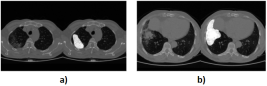
Figure 1: (a,b): CT Slice (Left), Free hand annotated CT Slice (Right)

Dataset	Number of CT Scans	Number of Slices
Training	126	56387
Validation	20	9992
Test	36	14727

Table 1: Scan-level and Slice-level Dataset splits

The positive class COVID-19 comprised consolidation and ground-glass opacities. These chest CT scans were divided into train, validation, and test datasets whose splits are given in Table 1.

The prevalence for all the datasets is 20%, which means that there are 20% positive slices in the total dataset. We resized all the images to a standard image size of (512, 512). Windowing, also known as grey-level mapping is the pre-processing of CT scans in which the grey-scale component of the CT slice is changed to highlight some particular features. We applied windowing to our scans lee2018practical , for which we used the information stored in the metadata from the DICOM files of the CT scans’ slices. The masks were stored as binary images of size (512, 512). The distribution of the number of slices in these CT scans for the whole dataset can be visualized from the histogram in Figure 2

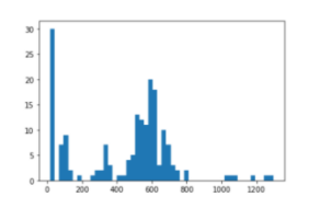
Figure 2: Volume variation in the CT scans for the whole dataset

4 Methodology

In this paper, we follow two approaches to address image segmentation of these CT scans:

4.1 2D Approach

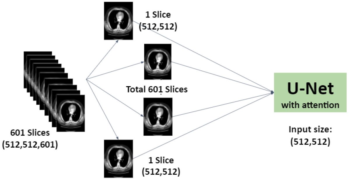
Figure 3: 2D Technique

In this approach, we divide the CT scan volume into separate 2D slices (Figure 3). For example, a CT scan of volume (512, 512, 601) containing 601 slices was divided into 601 individual images of (512, 512). We used the U-net with the Convolutional Block Attention Module (CBAM) woo2018cbam to focus its attention on a region of the image and then segment the pathology from that region of the image. U-Nets are fully convolutional networks having skip connections between encoder and decoder which provide deconvolution layers with important features hesamian2019deep . We used Xception chollet2017xception as the encoder having depthwise separable convolutions and residual connections. The model was trained using ADAM as its optimizer with an initial learning rate of 1e-3 and having a learning rate scheduler which reduced the learning rate to 1/3 the original learning rate, every 5 epochs. We used dice loss as the loss function. Our architecture had 38 million trainable parameters.

4.2 3D Approach

In the 3D approach, instead of assigning 2D images as the input for the model, we provide 3D volumes as to input for the model, and the corresponding stacked annotated slices as the label. For our 3D approach, we use V-Net milletari2016v , which is a 3D implementation of U-Net. For our input size of (512, 512, 32); V-Net had 206 million trainable parameters. We used the dice loss as the loss function while training. The model was trained using ADAM as its optimizer with an initial learning rate of 1e-3 and having a learning rate scheduler which reduced the learning rate to 1/3 the original learning rate every 5 epochs. The input to V-Net is volumetric data of dimension (x, y, z) = (512, 512, 32) where x is slice’s height, y is slice’s width, and z is the number of slices in the depth of the volume. To prepare the input data for training V-Net, we normalize the volume of the CT scans to the same value, having a dimension equal to the input dimension of the model. To satisfy this condition without losing any information, we split CTs into smaller volumes that match the input dimensions. We can see the CT scan being split into multiple stacks of slices in Figure 4.

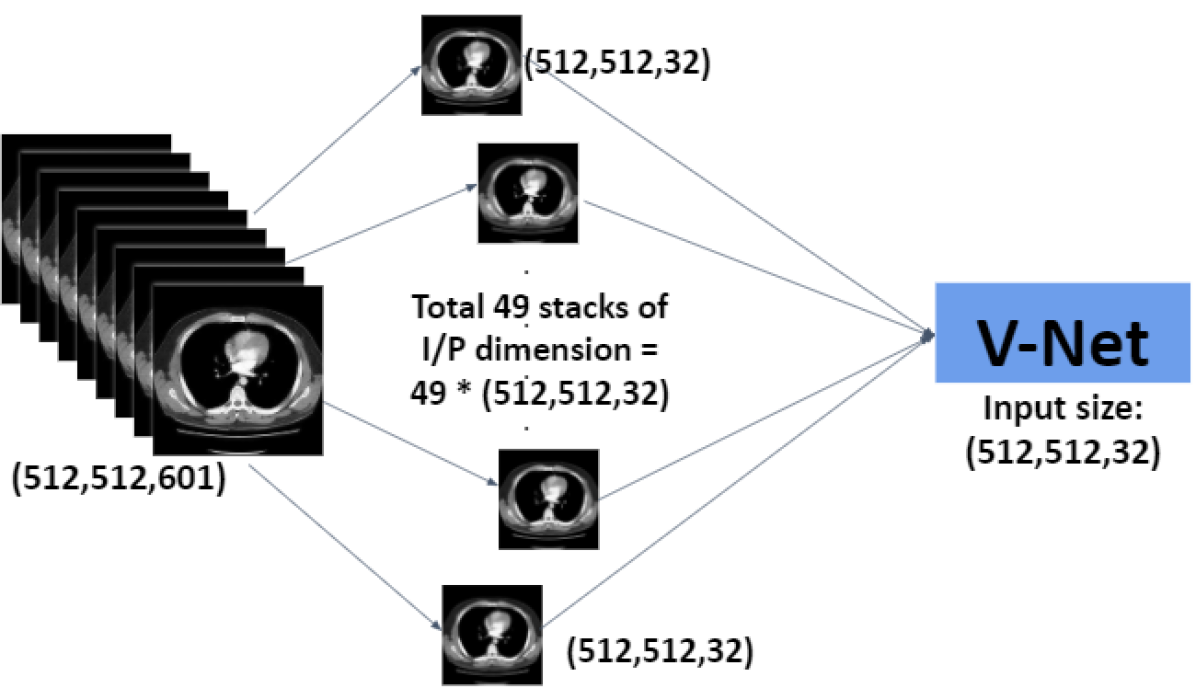
Figure 4: 3D Technique

There are three variables that affect the stacks creation process.
1. CT Volume: Number of slices in the CT scan
2. Stack size: Desired number of slices in the sub volume
3.Overlap factor = (Number of overlapping slices/stack size) Where overlapping slices is the number of slices that are common or overlapping in adjacent stacks.

For a CT scan having 601 slices, with a stack size of 32, and the number of overlapping slices as 20 (overlap factor = 0.625), we get a list of 49 stacks having dimensions (512, 512, 32). The first stack will have indices from 0 to 32, which means that the first input datapoint for V-Net will be a CT sub volume from the 1st slice to the 32nd slice. The second input data point will be a sub volume of the CT from index 12 to 44, both inclusive. As we have 20 overlapping slices, the second stack starts from the 12th index and not the 33rd. And so on for the rest of the stacks. For the last stack, however, the indices are (576, 608), the 7 extra slices are the added paddings to keep the volume of the stack compatible with the 3D model’s input dimension. During the inference, we keep the overlap factor as 0, the list of predicted mask volumes are then stacked together. So during the inference evaluation, we have a total of 19 stacks grouped. We remove the padding when the predictions are stacked together to match the volume of the whole CT scan.

5 Results

We evaluate the 2D and the 3D model based on these 5 criteria.

5.1 Dice Score

We predicted masks for 32 scans in the test set having a prevalence of 20% and calculated the dice score for the whole dataset. We observed the dice scores given in Table 2.

Model	Dice Score
2D Model	73%
3D Model	79%

Table 2: Dice Scores for 2D and 3D techniques

We took the average of the dice scores of these 32 scans. For the 2D model, we arranged the individual slices on top of each other to get the final predicted volume. For the 3D model, we combined the stacks of an individual CT and then removed the corresponding padding to match the true label volume.

5.2 Slices Predicted masks

Figure 5(a) and 5(b) show the predicted masks at the scan and slice level for 2D and the 3D model. We applied a threshold of 0.2 on the predictions.

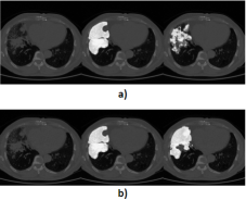
Figure 5: a)3D Model, b) 2D Model
Left=Original CT Slice, Middle = True label superimposed, Right = Predicted Mask superimposed

5.3 Area-plots

Here, we find the area of the annotated region with respect to the total area of the image. We normalize this list of area-ratios by dividing all the values by the maximum value in the list. Next, we plot these normalized values according to the slices in the CT scan to get the plot in Figure 6, these plots are called area-plots. We follow the same procedure for the predicted masks for 2D and 3D models, by plotting their normalized area-plots according to the position of the slices in the CT scan in Figure 7, 8 respectively. We have compared the predicted area-plots for both the 2D and the 3D approach to the area-plots of the true label.

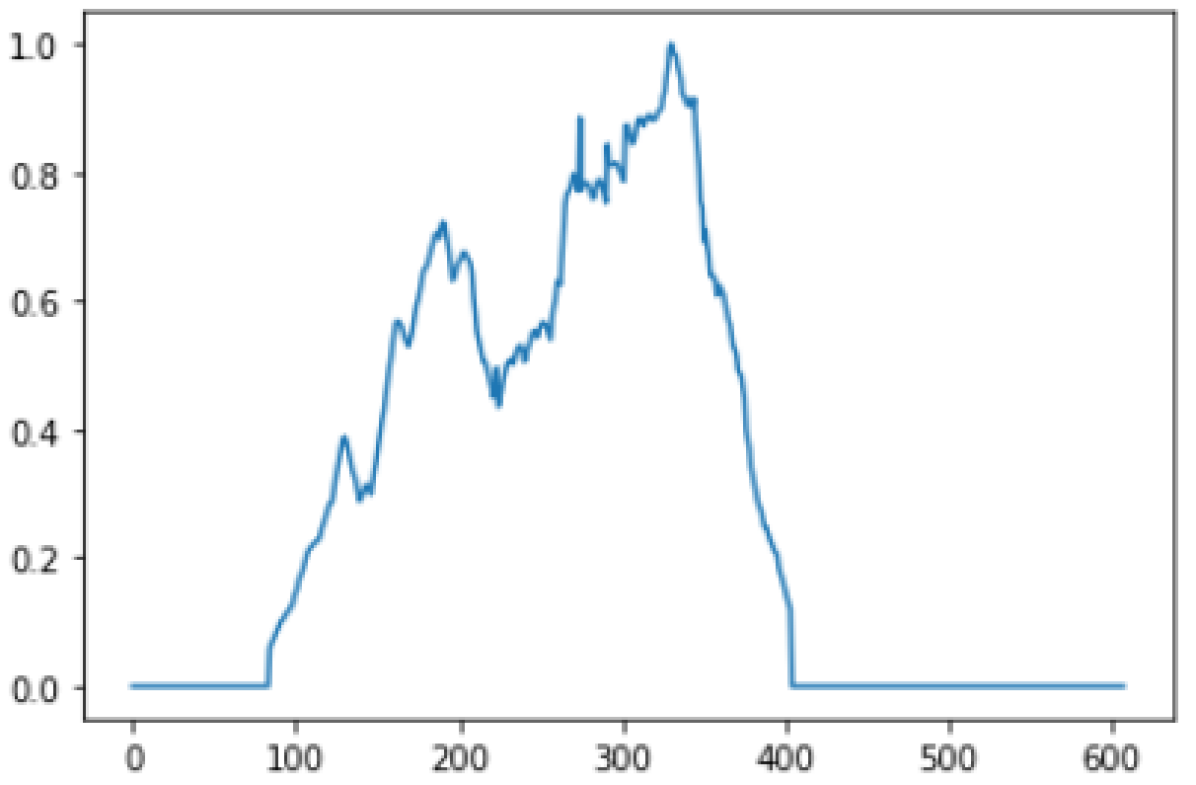
Figure 6: True Label’s Area-Plot

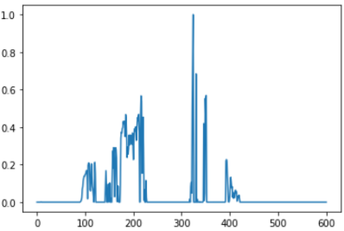
Figure 7: Area-Plot predicted by 2D Model

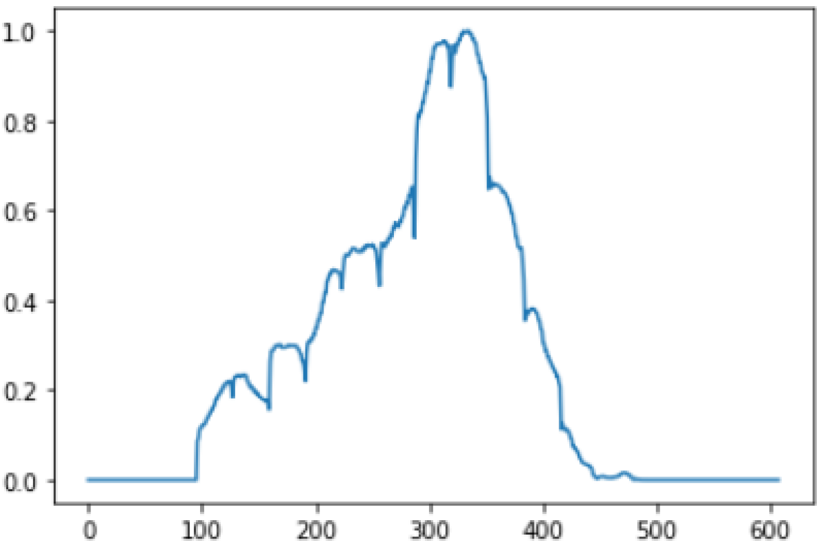
Figure 8: Area-Plot predicted by 3D Model

1. From Figure 6, we observe a continuous pattern in the manifestations of the pathology in the CT scan. Similar continuous patterns were observed for the rest of the CT scans, area-plots.
2. From Figure 7, we observe that there are abrupt variations in the predicted mask’s area for the slices within a CT scan when we use the 2D approach.
3. From Figure 8, we can see the prediction area-plot for a CT scan when using the 3D approach. We observe a smooth and continuous pattern in the masks predicted by the 3D model for the slices of that CT scan.

To further prove and understand point number 2, we plotted the predicted masks for consecutive slices in a CT scan using 2D and the 3D approach.

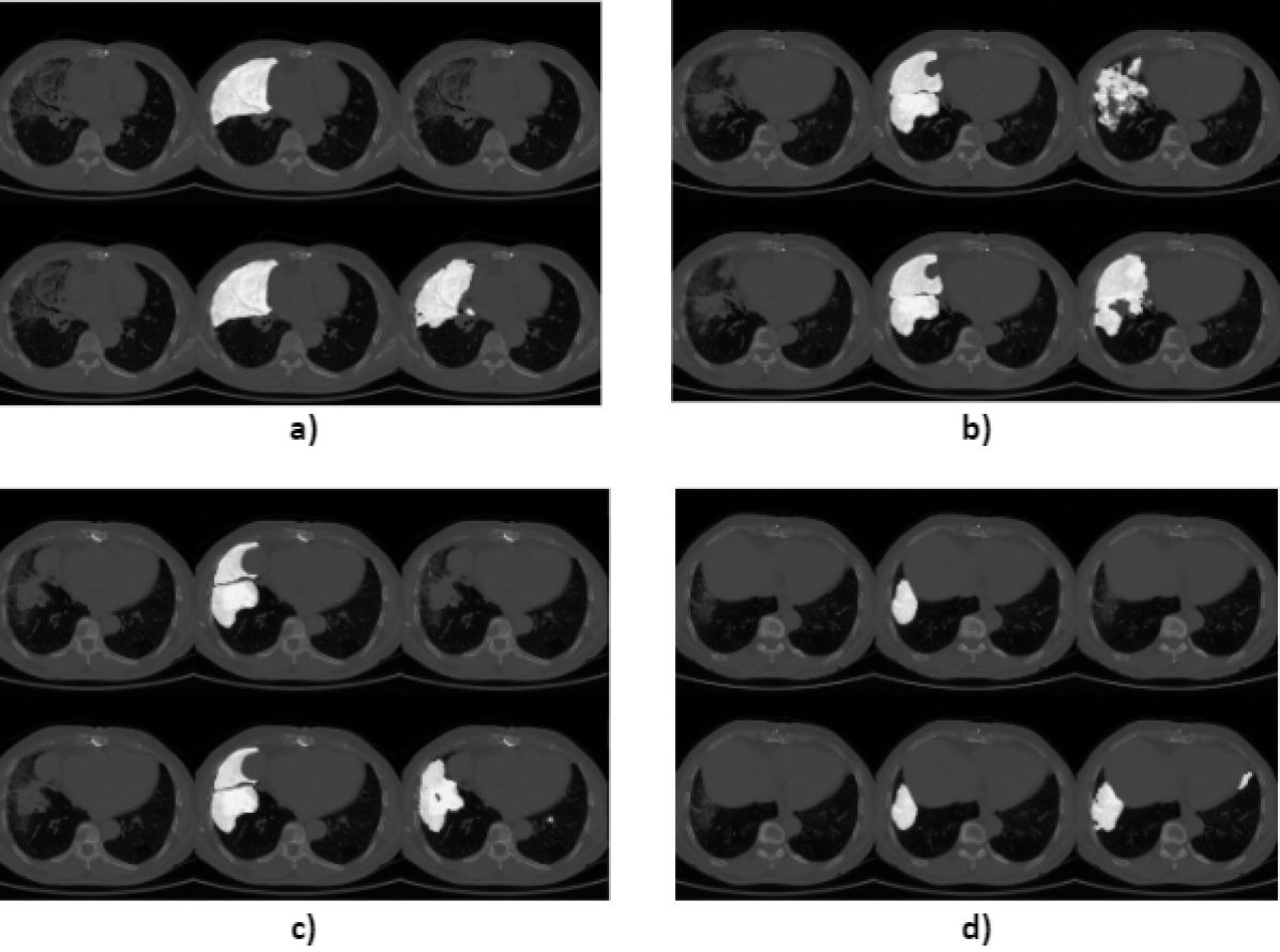
Figure 9: Predicted masks in four consecutive slices (a, b, c, d).
Left: Original slice, Middle: True Mask, Right: Predicted Mask
2D (top 3 images) and 3D (bottom 3 images)

For the four consecutive positive slices that we chose, the 3D model predicted all the slices as positive, i.e.(1,1,1,1), whereas, in the case of the 2D model, the predictions were (0,1,0,0). From Figure 9, we observe that the 3D approach predicted the masks in all 4 consecutive slices to closely match the labels. This represents the continuity in the predictions. We also observe that the shape or the area of the predicted masks do not change abruptly when we look at the adjacent slices. Although, in the masks predicted by the 2D approach, we observe that only some of the slices were marked positive. This represents the discontinuity in the predicted masks’ pattern. It indicates that the 2D approach does not consider the slices’ information adjacent to the input slice, thus giving us this abrupt predicted pattern, which is independent of the slices above and below the current slice.

5.4 Inference time

We calculate the inference time for 2D as well as 3D techniques for a CT scan.

Technique	Inference time	Inference time
	With GPU	Without GPU
2D	70	1145
3D	17	229

Table 3: Inference time for 2D and 3D techniques in seconds

Table 3 shows the inference time for a single CT scan having 709 slices with a stack size of 32 and an image size of (512, 512). We observe that there is a boost up of 5X in the 3D approach as compared to the 2D approach. For inference, we used a Tesla T4 GPU with 15GB of memory.

5.5 Overlap Variation

In this experiment, we changed the overlap factor to see its effect on the predictions. We kept the overlap factor as 0, 0.375, and 0.625. The predicted area-plots are given in Figure 11, 12, 13 respectively and the predicted masks are given in fig 14(a), 14(b), and 14(c) respectively. Figure 10 shows the true area-plot for the same CT scan.

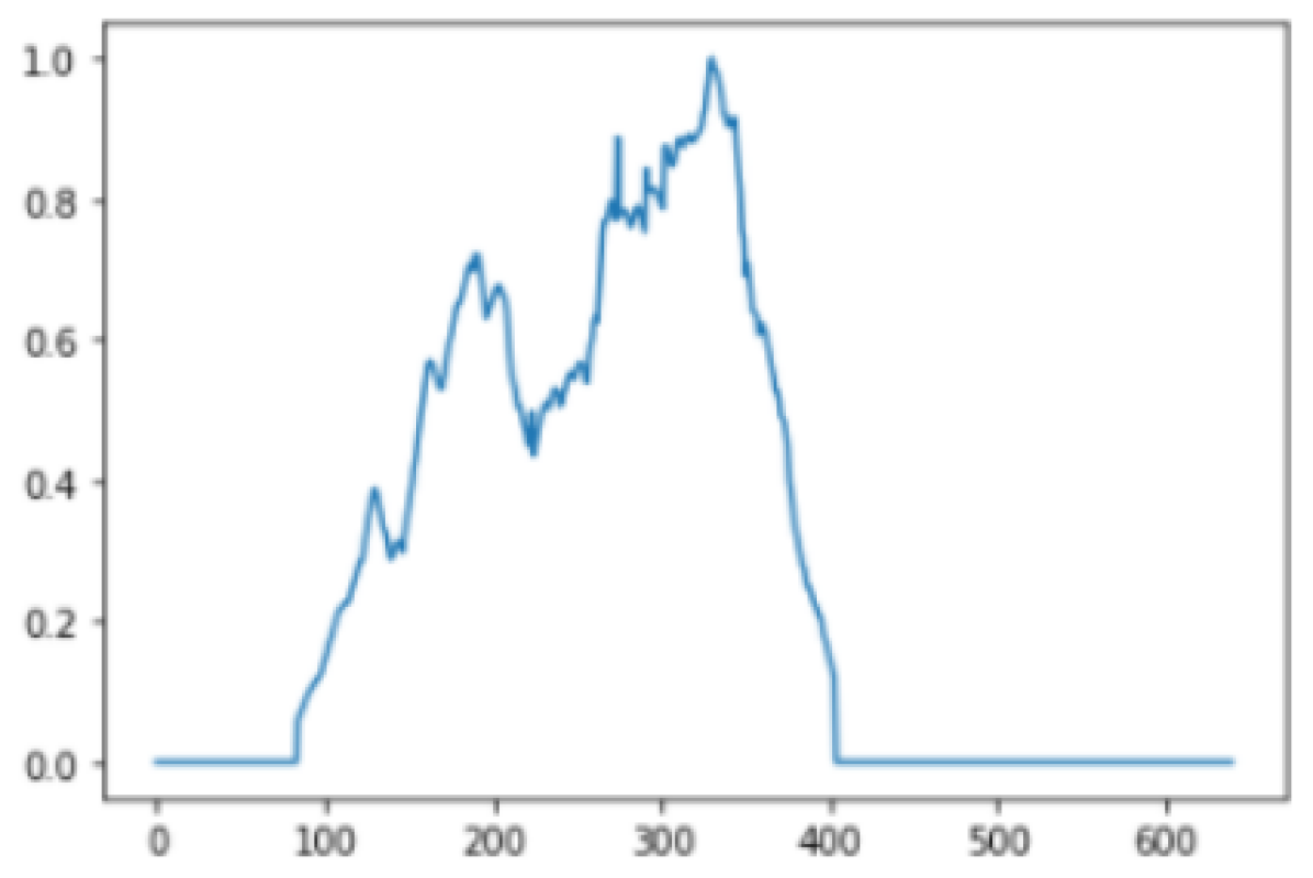
Figure 10: True Label’s Area-Plot

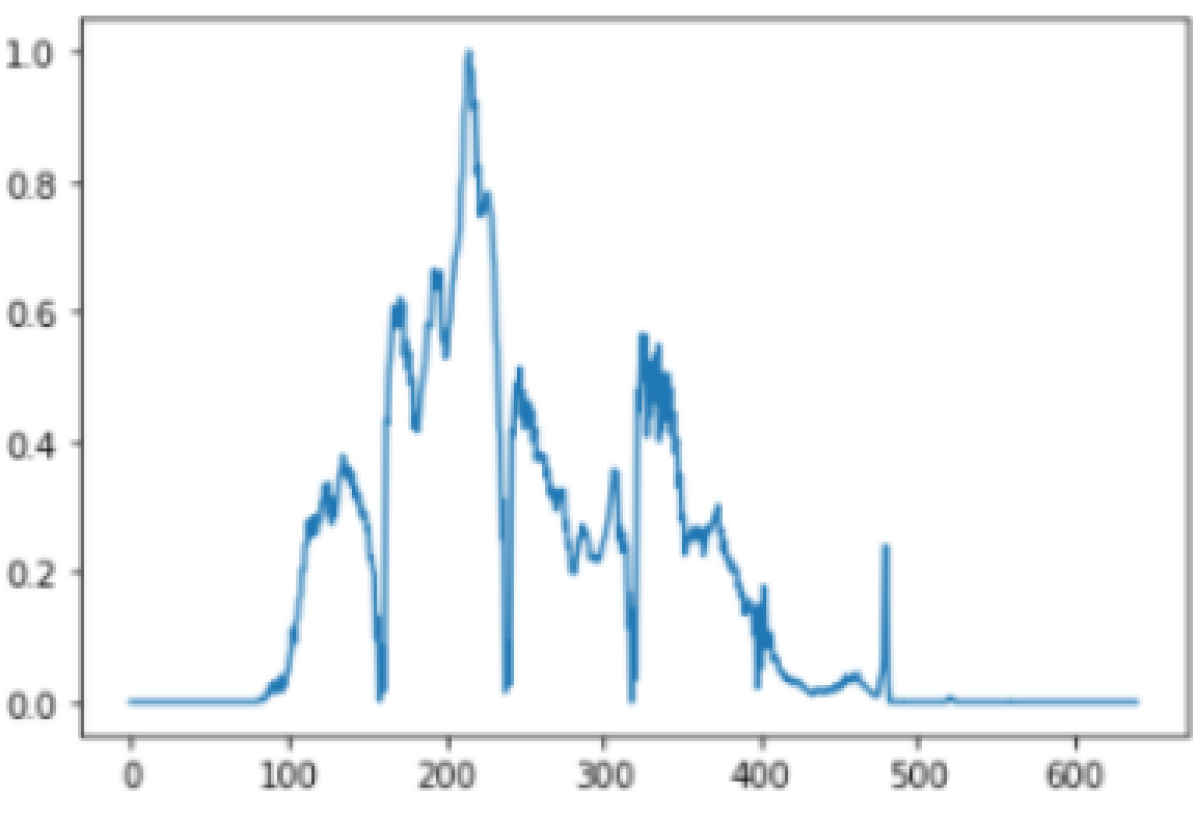
Figure 11: Area-Plot predicted by 3D Model, with overlap factor = 0

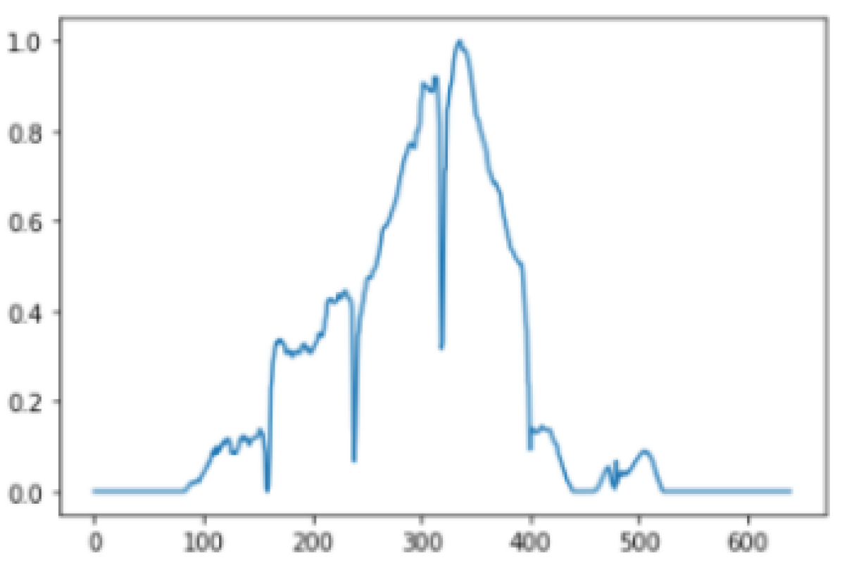
Figure 12: Area-Plot predicted by 3D Model, with overlap factor = 0.375

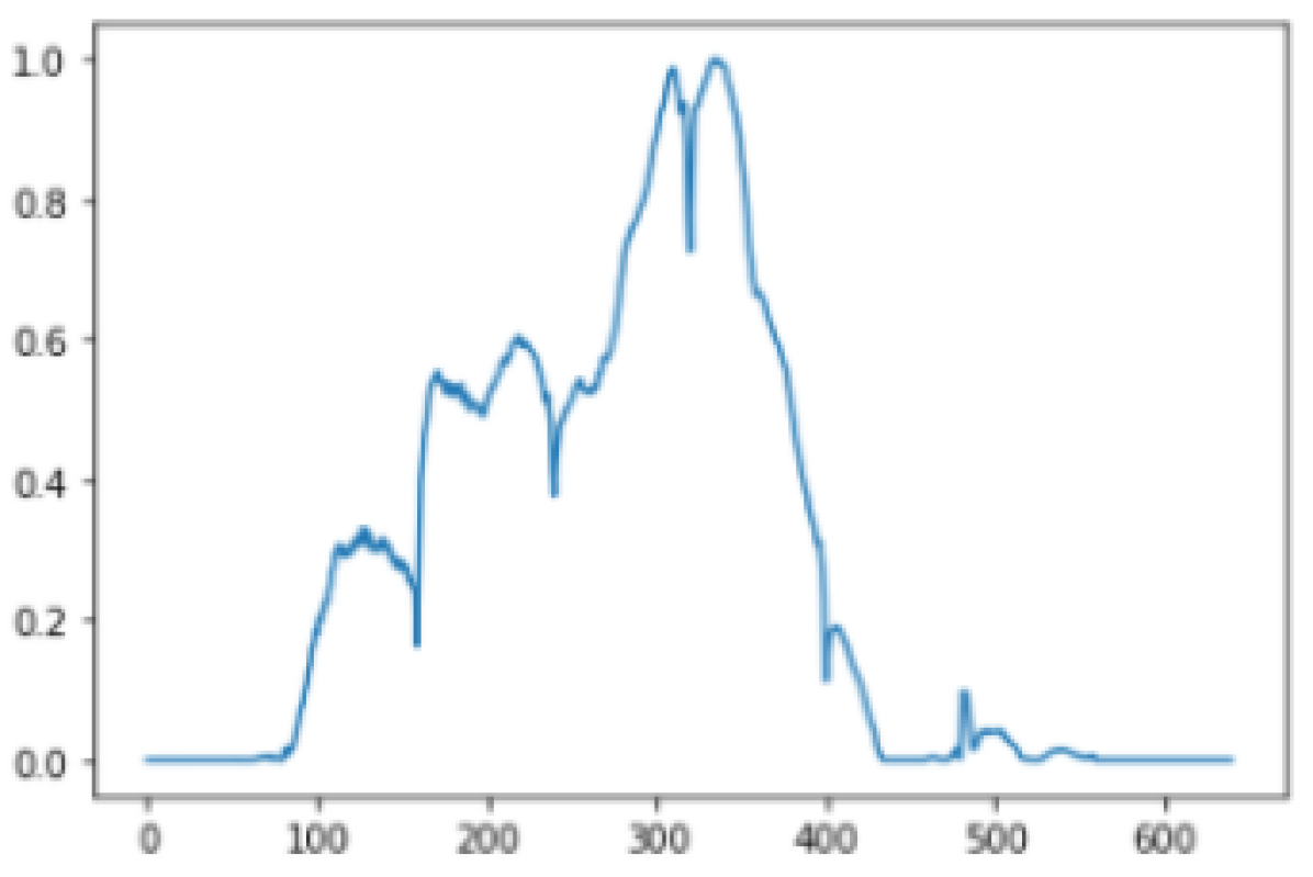
Figure 13: Area-Plot predicted by 3D Model, with overlap factor = 0.625

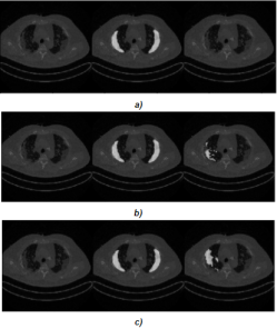
Figure 14: Predicted mask for the same slice having (a) overlap factor = 0, (b)overlap factor = 0.375, (c) overlap factor = 0.625
Left: Original slice, Middle: True Mask, Right: Predicted Mask

As we increase the overlap factor, the number of overlapping slices increases. This allows the model to interpret more global features. We observe that the predicted area-plots in Figure 14 with an overlap factor 0.625 match closely to the true area-plots in Figure 10. This shift in the pattern from Figure 11 to Figure 13 demonstrates that increasing the amount of contextual information retained allows the model to perform better thus giving closer predictions to the ground truth.

6 Conclusion

We implement and compare two deep learning approaches for segmenting out manifestations of consolidation and ground-glass-opacities in CT scans on three major grounds: predicted masks or the segmentation results, the pattern observed in the area of the predicted masks in a CT scan, and the inference time.

We saw that the 3D approach provided us with a better dice score than the 2D approach, thus proving to be more accurate at segmenting pathology regions. We also observed from Figure 8 that the area-plots we get using the 3D approach match closely to the original annotation area-plots against the area-plots of the 2D approach. We attribute these peculiar predicted patterns in the area-plots to the contextual information retained in the 3D stack volumes used to train the 3D model. The independent nature of the input images in the 2D model could be the reason for a discontinuous pattern in the predicted area-plots of the 2D approach. When we calculated the inference time, the 3D approach provided a boost of 5X in inference time compared to that of the 2D approach This is hugely beneficial for effective and quick diagnosis of patients in hospital settings especially the Intensive Care Units(ICUs). We conclude that this 3D stack-based approach is a better choice than the conventional 2D approach.

Later, when we experimented with the overlap factor for the 3D approach, the predicted area-plots’ patterns changed (Figure 11, 12, 13) with increasing overlap factor. However, a higher overlap factor may result in overfitting the model to the given dataset. The model gets more susceptible to a covariance-shift in the case of out-of-sample datasets when the overlap factor is high. Thus, the overlap factor should be treated as a hyperparameter for this 3D approach and should be set optimally.

Usually, in the case of 3D segmentation for CT scans, the whole CT scan is compressed using spline interpolation milletari2016v , or other methods, to the size of input dimension for a 3D model. This removes useful information when compressed for training and adds noise when decompressed for inference hahn2016comparison . To counter this alteration in the original data, we split the CT into smaller stacks to retain the valuable contextual information. Thus, our batch-based 3D approach is highly adaptable to any CT volume because of its stack-based nature, where none of the information between the slices in the CT is altered.

The segmentation results can be improved using more data, and different augmentation techniques while training. In our case study, the goal was to compare the 2D and the 3D approaches on equal grounds, and not the segmentation result itself. In conclusion, the 3D approach that has been proposed in this paper has outperformed the traditional 2D approach in all the three criteria that we had set for evaluation.

References

- (1) A. Umar and S. Atabo, “A review of imaging techniques in scientific research/clinical diagnosis,” MOJ Anat & Physiol, vol. 6, no. 5, pp. 175–183, 2019.
- (2) C. for Disease Control, Prevention, et al., “Pneumonia can be prevented–vaccines can help,” 2012.
- (3) J. Zhang, Y. Xie, Z. Liao, G. Pang, J. Verjans, W. Li, Z. Sun, J. He, Y. Li, C. Shen, et al., “Viral pneumonia screening on chest x-ray images using confidence-aware anomaly detection,” arXiv preprint arXiv:2003.12338, vol. 3, 2020.
- (4) K. Doi, “Computer-aided diagnosis in medical imaging: historical review, current status and future potential,” Computerized medical imaging and graphics, vol. 31, no. 4-5, pp. 198–211, 2007.
- (5) O. H. Karatas and E. Toy, “Three-dimensional imaging techniques: A literature review,” European journal of dentistry, vol. 8, no. 1, p. 132, 2014.
- (6) L. Rodríguez-Mazahua, C.-A. Rodríguez-Enríquez, J. L. Sánchez-Cervantes, J. Cervantes, J. L. García-Alcaraz, and G. Alor-Hernández, “A general perspective of big data: applications, tools, challenges and trends,” The Journal of Supercomputing, vol. 72, no. 8, pp. 3073–3113, 2016.
- (7) M. Minsky, “Steps toward artificial intelligence,” Proceedings of the IRE, vol. 49, no. 1, pp. 8–30, 1961.
- (8) I. M. Cockburn, R. Henderson, and S. Stern, “The impact of artificial intelligence on innovation,” tech. rep., National bureau of economic research, 2018.
- (9) L. Yang, “Research on application of artificial intelligence based on big data background in computer network technology,” Journal of Jiujiang Vocational & Technical College, vol. 392, no. 6, 2018.
- (10) Y. Lu and S. Young, “A survey of public datasets for computer vision tasks in precision agriculture,” Computers and Electronics in Agriculture, vol. 178, p. 105760, 2020.
- (11) M. D. Kohli, R. M. Summers, and J. R. Geis, “Medical image data and datasets in the era of machine learning—whitepaper from the 2016 c-mimi meeting dataset session,” Journal of digital imaging, vol. 30, no. 4, pp. 392–399, 2017.
- (12) R. Smith-Bindman, Y. Wang, P. Chu, R. Chung, A. J. Einstein, J. Balcombe, M. Cocker, M. Das, B. N. Delman, M. Flynn, et al., “International variation in radiation dose for computed tomography examinations: prospective cohort study,” Bmj, vol. 364, 2019.
- (13) S. Trattner, G. D. Pearson, C. Chin, D. D. Cody, R. Gupta, C. P. Hess, M. K. Kalra, J. M. Kofler Jr, M. S. Krishnam, and A. J. Einstein, “Standardization and optimization of ct protocols to achieve low dose,” Journal of the American College of Radiology, vol. 11, no. 3, pp. 271–278, 2014.
- (14) Z. Xue, S. Antani, L. R. Long, D. Demner-Fushman, and G. R. Thoma, “Window classification of brain ct images in biomedical articles,” in AMIA Annual Symposium Proceedings, vol. 2012, p. 1023, American Medical Informatics Association, 2012.
- (15) M. J. Willemink and P. B. Noël, “The evolution of image reconstruction for ct—from filtered back projection to artificial intelligence,” European radiology, vol. 29, no. 5, pp. 2185–2195, 2019.
- (16) Q. Yang, P. Yan, Y. Zhang, H. Yu, Y. Shi, X. Mou, M. K. Kalra, Y. Zhang, L. Sun, and G. Wang, “Low-dose ct image denoising using a generative adversarial network with wasserstein distance and perceptual loss,” IEEE transactions on medical imaging, vol. 37, no. 6, pp. 1348–1357, 2018.
- (17) I. R. I. Haque and J. Neubert, “Deep learning approaches to biomedical image segmentation,” Informatics in Medicine Unlocked, vol. 18, p. 100297, 2020.
- (18) X. Zhou, K. Yamada, T. Kojima, R. Takayama, S. Wang, X. Zhou, T. Hara, and H. Fujita, “Performance evaluation of 2d and 3d deep learning approaches for automatic segmentation of multiple organs on ct images,” in Medical Imaging 2018: Computer-Aided Diagnosis, vol. 10575, p. 105752C, International Society for Optics and Photonics, 2018.
- (19) A. D. Weston, P. Korfiatis, T. L. Kline, K. A. Philbrick, P. Kostandy, T. Sakinis, M. Sugimoto, N. Takahashi, and B. J. Erickson, “Automated abdominal segmentation of ct scans for body composition analysis using deep learning,” Radiology, vol. 290, no. 3, pp. 669–679, 2019.
- (20) W. Zhao, D. Jiang, J. P. Queralta, and T. Westerlund, “Mss u-net: 3d segmentation of kidneys and tumors from ct images with a multi-scale supervised u-net,” Informatics in Medicine Unlocked, p. 100357, 2020.
- (21) A. Akbik, D. Blythe, and R. Vollgraf, “Contextual string embeddings for sequence labeling,” in Proceedings of the 27th International Conference on Computational Linguistics, pp. 1638–1649, 2018.
- (22) A. Hassan and A. Mahmood, “Deep learning for sentence classification,” in 2017 IEEE Long Island Systems, Applications and Technology Conference (LISAT), pp. 1–5, IEEE, 2017.
- (23) C. Olah and S. Carter, “Attention and augmented recurrent neural networks,” Distill, vol. 1, no. 9, p. e1, 2016.
- (24) M.-S. Badea, I.-I. Felea, L. M. Florea, and C. Vertan, “The use of deep learning in image segmentation, classification and detection,” arXiv preprint arXiv:1605.09612, 2016.
- (25) Y. LeCun, L. Bottou, Y. Bengio, and P. Haffner, “Gradient-based learning applied to document recognition,” Proceedings of the IEEE, vol. 86, no. 11, pp. 2278–2324, 1998.
- (26) M. Lin, Q. Chen, and S. Yan, “Network in network,” arXiv preprint arXiv:1312.4400, 2013.
- (27) M. Polsinelli, L. Cinque, and G. Placidi, “A light cnn for detecting covid-19 from ct scans of the chest,” arXiv preprint arXiv:2004.12837, 2020.
- (28) T. Okada, M. G. Linguraru, M. Hori, R. M. Summers, N. Tomiyama, and Y. Sato, “Abdominal multi-organ segmentation from ct images using conditional shape–location and unsupervised intensity priors,” Medical image analysis, vol. 26, no. 1, pp. 1–18, 2015.
- (29) V. Badrinarayanan, A. Kendall, and R. Cipolla, “Segnet: A deep convolutional encoder-decoder architecture for image segmentation,” IEEE transactions on pattern analysis and machine intelligence, vol. 39, no. 12, pp. 2481–2495, 2017.
- (30) O. Ronneberger, P. Fischer, and T. Brox, “U-net: Convolutional networks for biomedical image segmentation,” in International Conference on Medical image computing and computer-assisted intervention, pp. 234–241, Springer, 2015.
- (31) P. F. Christ, F. Ettlinger, F. Grün, M. E. A. Elshaera, J. Lipkova, S. Schlecht, F. Ahmaddy, S. Tatavarty, M. Bickel, P. Bilic, et al., “Automatic liver and tumor segmentation of ct and mri volumes using cascaded fully convolutional neural networks,” arXiv preprint arXiv:1702.05970, 2017.
- (32) S. Almotairi, G. Kareem, M. Aouf, B. Almutairi, and M. A.-M. Salem, “Liver tumor segmentation in ct scans using modified segnet,” Sensors, vol. 20, no. 5, p. 1516, 2020.
- (33) X. ZHOU, T. ITO, R. TAKAYAMA, S. WANG, T. HARA, and H. FUJITA, “First trial and evaluation of anatomical structure segmentations in 3d ct images based only on deep learning,” Medical Imaging and Information Sciences, vol. 33, no. 3, pp. 69–74, 2016.
- (34) J. Long, E. Shelhamer, and T. Darrell, “Fully convolutional networks for semantic segmentation,” in Proceedings of the IEEE conference on computer vision and pattern recognition, pp. 3431–3440, 2015.
- (35) A. de Brebisson and G. Montana, “Deep neural networks for anatomical brain segmentation,” in Proceedings of the IEEE conference on computer vision and pattern recognition workshops, pp. 20–28, 2015.
- (36) H. R. Roth, A. Farag, L. Lu, E. B. Turkbey, and R. M. Summers, “Deep convolutional networks for pancreas segmentation in ct imaging,” in Medical Imaging 2015: Image Processing, vol. 9413, p. 94131G, International Society for Optics and Photonics, 2015.
- (37) K. H. Cha, L. Hadjiiski, R. K. Samala, H.-P. Chan, E. M. Caoili, and R. H. Cohan, “Urinary bladder segmentation in ct urography using deep-learning convolutional neural network and level sets,” Medical physics, vol. 43, no. 4, pp. 1882–1896, 2016.
- (38) X. Zhou, T. Ito, R. Takayama, S. Wang, T. Hara, and H. Fujita, “Three-dimensional ct image segmentation by combining 2d fully convolutional network with 3d majority voting,” in Deep Learning and Data Labeling for Medical Applications, pp. 111–120, Springer, 2016.
- (39) A. Kayid, Y. Khaled, and M. Elmahdy, “Performance of cpus/gpus for deep learning workloads,” The German University in Cairo, 2018.
- (40) Ö. Çiçek, A. Abdulkadir, S. S. Lienkamp, T. Brox, and O. Ronneberger, “3d u-net: learning dense volumetric segmentation from sparse annotation,” in International conference on medical image computing and computer-assisted intervention, pp. 424–432, Springer, 2016.
- (41) F. Milletari, N. Navab, and S.-A. Ahmadi, “V-net: Fully convolutional neural networks for volumetric medical image segmentation,” in 2016 fourth international conference on 3D vision (3DV), pp. 565–571, IEEE, 2016.
- (42) H. Chen, Q. Dou, L. Yu, and P.-A. Heng, “Voxresnet: Deep voxelwise residual networks for volumetric brain segmentation,” arXiv preprint arXiv:1608.05895, 2016.
- (43) N. Alalwan, A. Abozeid, A. A. ElHabshy, and A. Alzahrani, “Efficient 3d deep learning model for medical image semantic segmentation,” Alexandria Engineering Journal, vol. 60, no. 1, pp. 1231–1239.
- (44) X. Li, H. Chen, X. Qi, Q. Dou, C.-W. Fu, and P.-A. Heng, “H-denseunet: hybrid densely connected unet for liver and tumor segmentation from ct volumes,” IEEE transactions on medical imaging, vol. 37, no. 12, pp. 2663–2674, 2018.
- (45) K. Simonyan and A. Zisserman, “Very deep convolutional networks for large-scale image recognition,” arXiv preprint arXiv:1409.1556, 2014.
- (46) M. Chung, A. Bernheim, X. Mei, N. Zhang, M. Huang, X. Zeng, J. Cui, W. Xu, Y. Yang, Z. A. Fayad, et al., “Ct imaging features of 2019 novel coronavirus (2019-ncov),” Radiology, vol. 295, no. 1, pp. 202–207, 2020.
- (47) P. A. Yushkevich, Y. Gao, and G. Gerig, “Itk-snap: An interactive tool for semi-automatic segmentation of multi-modality biomedical images,” in 2016 38th Annual International Conference of the IEEE Engineering in Medicine and Biology Society (EMBC), pp. 3342–3345, IEEE, 2016.
- (48) H. Lee, M. Kim, and S. Do, “Practical window setting optimization for medical image deep learning,” arXiv preprint arXiv:1812.00572, 2018.
- (49) S. Woo, J. Park, J.-Y. Lee, and I. So Kweon, “Cbam: Convolutional block attention module,” in Proceedings of the European conference on computer vision (ECCV), pp. 3–19, 2018.
- (50) M. H. Hesamian, W. Jia, X. He, and P. Kennedy, “Deep learning techniques for medical image segmentation: Achievements and challenges,” Journal of digital imaging, vol. 32, no. 4, pp. 582–596, 2019.
- (51) F. Chollet, “Xception: Deep learning with depthwise separable convolutions,” in Proceedings of the IEEE conference on computer vision and pattern recognition, pp. 1251–1258, 2017.
- (52) K. Hahn, H. Schöndube, K. Stierstorfer, J. Hornegger, and F. Noo, “A comparison of linear interpolation models for iterative ct reconstruction,” Medical physics, vol. 43, no. 12, pp. 6455–6473, 2016.