Large Area X-ray Proportional Counter (LAXPC) in Orbit Performance : Calibration, background, analysis software

Abstract

The Large Area X-ray Proportional Counter (LAXPC) instrument on-board AstroSat has three nominally identical detectors for timing and spectral studies in the energy range of 3–80 keV. The performance of these detectors during the five years after the launch of AstroSat is described. Currently, only one of the detector is working nominally. The variation in pressure, energy resolution, gain and background with time are discussed. The capabilities and limitations of the instrument are described. A brief account of available analysis software is also provided.

antia@tifr.res.in

1 Introduction

The Large Area X-ray Proportional Counter (LAXPC) instrument on-board AstroSat (Agrawal 2006; Singh et al. 2014) consists of three co-aligned detectors for X-ray timing and spectral studies over an energy range of 3–80 keV (Yadav et al. 2016a; Agrawal et al. 2017). Apart from LAXPC, AstroSat has three more co-aligned instruments, the Soft X-ray Telescope (SXT, Singh et al. 2016), the Cadmium Zinc Telluride Imager (CZTI, Bhalerao et al. 2017) and the Ultra-Violet Imaging Telescope (UVIT, Tandon et al. 2017). AstroSat was conceived to carry out multiwavelength observations of various sources in the Visible, UV and X-ray bands using these co-aligned instruments. AstroSat was launched on September 28, 2015 and the initial calibration of the LAXPC instrument was discussed by Antia et al. (2017). By now AstroSat has made more than 2000 distinct observations covering a wide variety of sources and a large amount of data are publicly available from the AstroSat Data Archive. A quick look light-curves of all LAXPC observations are available at the LAXPC website. A number of science results from LAXPC instrument have been published and a summary of these results is described in the companion paper (Yadav et al. 2020).

Each LAXPC detector has five layers divided into seven anodes (A1–A7), with the two top layers having two anodes each. In addition there are three veto anodes (A8–A10) on the three sides of the detector. The three faces covered by veto anodes are, the bottom and the two faces covering the long side of the detector as shown in Figure 2 of Antia et al. (2017). By default the LAXPC detectors operate in the Event Analysis (EA) mode where the timing and energy of each photon is recorded with the time-resolution of 10 $\mu$s. The EA mode operation also generates the Broad Band Counting (BB) mode data, which gives the counts with a predefined time-bin, for various energy bins and anodes, including the counts of events beyond the Upper Level Discriminator (ULD) threshold (nominally at 80 keV). The dead-time of the detectors is 42 $\mu$s (Yadav et al. 2016b). In addition, there is a Fast Counter (FC) mode with a dead-time of about 10 $\mu$s to allow for observation of bright sources. In this mode only the counts with a fixed time-bin of 160 $\mu$s, as recorded in only the top layer of the detector in four predefined energy bins are available. However, this mode has not been used for any science observation and no software to analyse the data is available. As a result, this mode is not allowed to be configured by LAXPC users. Thus effectively only one mode covering both EA and BB is allowed.

In the xenon gas counters, a large fraction of incoming photons above 34.5 keV emit a fluorescence photon and depending on the cell geometry and filling pressure, the fluorescent photon may generate a second localized electron cloud in a different anode. Therefore, on board electronics is designed to recognise such correlated double events and the energy deposited in the two anodes is added. These are referred to as double events as opposed to single events, where all energy is deposited in one anode.

In this article, we mainly focus on the performance of the LAXPC instrument in orbit and its calibration and some software which is available for analysing data. The three LAXPC detectors are labelled as LAXPC10, LAXPC20 and LAXPC30. Currently, only LAXPC20 is working nominally. The rest of the paper is organised as follows: Section 2 describes the performance of detectors during the last five years. Section 3 describes the variation in background with time and some procedures to correct for these. Section 4 describes some capabilities and limitations of the detectors and their sensitivity. Section 5 describes some software for analysing the data. Section 6 describes the various science goals of LAXPC detectors and how they are met by the data obtained so far. Finally, Section 7 describes a summary of calibration and performance of detectors.

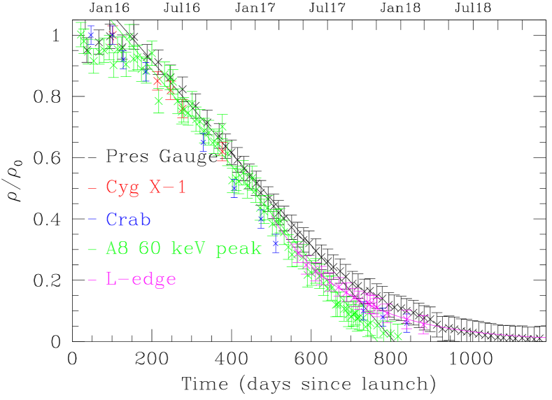
Figure 1: The pressure in LAXPC detectors as a function of time. The left panel shows the pressure as obtained from the pressure gauge for all three detectors. The right panel shows the density for LAXPC30 using various techniques. The dashed-line is the fit to linear part of the curve. Both pressure and density are shown relative to their initial values.

2 Long Term Performance of LAXPC in Orbit

The health parameters of the detectors, like the temperature, pressure, high voltage (HV) and various energy thresholds are monitored regularly. While the temperature of detectors is steady, the pressure has changed over the last five years from the initial value of about two atmospheres. The HV and thresholds have been maintained, except for some adjustments that were made from time to time. Further, to monitor the stability of detectors, the peak position and energy resolution of 30 and 60 keV peaks in the veto anode A8 from the on board radioactive source Am²⁴¹, are measured regularly and a log is maintained. Apart from these, we have also regularly monitored spectrum from Crab observation to check the stability of the detector response.

2.1 Pressure in Detectors

Figure 1, shows the pressure as estimated from the pressure gauge in all detectors as a function of time. The LAXPC30 developed a leak soon after launch and the pressure was decreasing steadily. The HV of the detector was turned off on March 8, 2018 when the pressure had reduced to about 5% of the original pressure. LAXPC10 also has a fine leak and the pressure has been reducing gradually. Curiously, the pressure gauge of LAXPC20 shows a slow increase in pressure. This is most likely an artefact and shows the limitation of on-board pressure gauge. Because of this, we used other techniques to estimate the density in LAXPC30, as described by Antia et al. (2017) and the results using these are shown in the right panel of Figure 1. Since these techniques are based on absorption in Xenon gas, they yield the density which is assumed to be a proxy for pressure, as the temperature is almost constant during the entire period. The Cyg X-1 observations during the soft state were used to measure the density by calibrating the ratio of counts around 20 keV, observed in different layers of the detector. The soft state was used to ensure very low flux beyond the Xe K-edge to avoid possible contamination from events involving Xe fluorescence photons. The Crab spectra were fitted using responses with different density to get the best fit for density. Other techniques were based on the strength of 60 keV peak in veto anode A8 and the observation of L-edge in the spectrum when the density was sufficiently low. It can be seen that results from all these techniques agree with each other. The density in LAXPC30 decreased linearly for some time at a rate of about 4.5% of original density per month. After that it followed an exponential rate, as may be expected for a leak, with an e-folding time of about 200 days. By now the pressure is below the sensitivity of pressure gauge and using the exponential profile it can be estimated to be about 0.05% of the original value. To maintain the gain of the detector in a reasonable limit the HV of detector was reduced from time to time. To allow analysis of LAXPC30 data, the response has been calculated at different densities and the software gives recommendation of which response to use depending on the time of observation.

2.2 Energy Resolution and Gain of Detectors

Because of the leak, the gain of LAXPC10 and LAXPC30 was also increasing with time and this needs to be estimated using the 30 keV line in the veto anode A8 from the Am²⁴¹ source. The calibration source has two lines, one at 30 keV due to K-escape event from Xe and another at 60 keV from the Am²⁴¹ source, and these peaks can be used to check the drift in gain as well as energy resolution. To correct for the drift in the gain, the HV of LAXPC10 and LAXPC30 was adjusted from time to time. This gives some steps in the gain. After some stage the gain of LAXPC30 had to be adjusted frequently, giving a band in the peak position as seen in the left panel of Figure 2. On January 22, 2018 the HV of LAXPC30 was reduced to the minimum possible value of about 930 V (as compared to the initial value of about 2300 V), after which the peak channel kept shifting upwards. Even before this stage, the 60 keV peak was not well defined due to low efficiency and hence its position could not be determined. By the time the HV of detector was turned off, even the 30 keV peak had shifted beyond the ULD and it was not possible to estimate the gain of the detector.

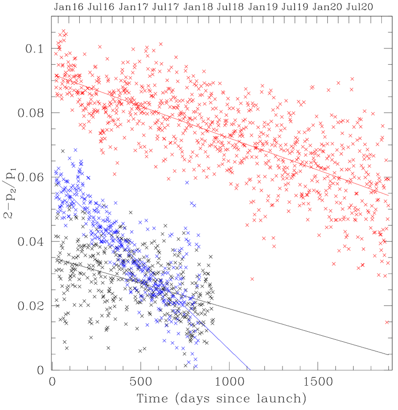
Figure 2: The energy resolution and peak channel for the 30 keV ($p_{1}$, as marked by cross) and 60 keV ($p_{2}$, as marked by open squares) calibration peak in veto anode A8 is shown in the left panel. The black, red and blue points show the result for LAXPC10, LAXPC20 and LAXPC30, respectively. The right panel shows the quantity $2-p_{2}/p_{1}$ for the three detectors. The lines mark the best fit straight lines for the three detectors.

The channel to energy mapping is defined by a quadratic (Antia et al. 2017) and it is not possible to estimate the three coefficients of quadratic using the peak position of two peaks. Hence, it is assumed that only the linear term is changing with time and its value is estimated by the position of the 30 keV peak. Responses for different values of the peak position of 30 keV peak are provided and software makes appropriate recommendation based on the time of observation. If the gain was linear the peak channel for 60 keV peak, $p_{2}$ would be twice that for 30 keV peak, $p_{1}$. Hence, the difference $2-p_{2}/p_{1}$ gives a measure of non-linearity in the gain. This quantity is shown in the right panel of Figure 2. It can be seen that the nonlinearity has been decreasing for all detectors. However, it should be noted that this quantity can also change if the constant term in the gain is changing. Thus it is not possible to correct for this variation. It is advisable to use gain fit command in Xspec to adjust the constant term, and even the linear term, to get the best spectral fit.

On March 26, 2018, LAXPC10 showed erratic counts with strong bursts where the dead-time corrected count rate reached 40000 s^-1. The cause of this anomaly is not known. To stabilise the counts, the HV of the detector was reduced. Attempts were also made to control the noise by adjusting the Low Level Discrimination (LLD) thresholds of some anodes which were showing low channel noise, but that did not remove the bursts and hence the HV was kept at lower value. After that the counts were stable to some extent though smaller bursts continued. By looking at the value of counts beyond the ULD it is possible to identify the time intervals when counts are not stable and this has been implemented in the software which automatically removes these time intervals from Good Time Intervals (GTI). This problem occurred a few times after that and every time the HV was reduced to stabilise the counts. The last adjustment was made on April 9, 2019 and since then no bursts have been observed, except for a few days between April 23 and May 3, 2020. Because of these adjustments, the HV of LAXPC10 has been reduced from about 2330 V initially to about 2190 V in March 2018 (before the anomalous behaviour started) and to 1860 V now. Some reduction in HV was also required to compensate for the leak in the detector. About half of the 470 V reduction would have been needed to compensate for the reduction in pressure. The status of LAXPC10 at any time can be checked on the LAXPC website. Even if the detector remains stable, it would take a few years for it to reach a reasonable gain due to leakage.

Because of the reduction in HV the energy thresholds of LAXPC10 have increased. At the time of last adjustment, the LLD was around 30 keV and ULD was about 400 keV. Since then because of the fine leak the thresholds have reduced to some extent, with LLD around 22 keV and ULD around 320 keV. It is difficult to estimate the gain of this detector reliably and to get the corresponding response. As a result, it is not possible to use this detector for spectroscopic studies. During the period just after March 26, 2018 the gain of the detector was in a reasonable range. As a result, the data obtained during that interval could be analysed if single event mode for only the top layer of the detector is used. It is necessary to reject all double events where the energy is deposited in two different anodes due to Xe K X-ray photons being absorbed in a different anode, as the energy thresholds for choosing these events have not been adjusted due to difficulty in estimating them reliably. The restriction to top layer of detector is needed because the LLD threshold of some other anodes has been increased giving an edge in the spectrum.

Figure 3: The pulse profile of GRO J2058+42 as calculated from LAXPC10 data.

Even with the low gain, LAXPC10 does detect bursts, e.g., from GRB (Antia et al. 2020a,b). Similarly, it is possible to detect pulsation in LAXPC10, e.g., for GRO J2058+42 during its outburst in April 2019, the pulsation period was determined to be $194.256\pm 0.034$ s and spin-up rate was estimate to be $\dot{\nu}=(1.7\pm 1.0)\times 10^{-11}$ Hz s^-1. This can be compared with $P=194.2201\pm 0.0016$ s and $\dot{\nu}=(1.65\pm 0.06)\times 10^{-11}$ Hz s^-1 obtained with LAXPC20 (Mukerjee et al. 2020a). The error-bars represent the 90% confidence limits. The higher error in LAXPC10 is mainly due to lower counts because of higher LLD and low efficiency. This observation was taken at a time when the counts were not very stable in LAXPC10 and only about 7% of exposure time was usable. The pulse profile obtained from LAXPC10 is shown in Figure 3. The gain of the detector during this observation is uncertain and the LLD was probably around 30 keV. This pulse profile can be compared with pulse profile obtained for energy range 30–40 keV from LAXPC20 (Mukerjee et al. 2020a).

Figure 4: The results of fit to Crab spectrum observed during the last 5 years is shown as a function of days from launch of AstroSat for the three LAXPC detectors as marked in the figure. The different panels show all fitted parameters as well as the reduced $\chi^{2}$ for the fit.

The energy resolution of LAXPC10 was stable until March 2018, while that for LAXPC30 was improving with time, probably due to reduction in pressure. The energy resolution of LAXPC20 has been deteriorating with time and currently the resolution at 30 keV is about 20%. The position of peak channel in LAXPC20 has been steady and the last adjustment in HV was made on March 15, 2017. Since then the peak position has reduced by about 12 channels. Since this detector is already operating at higher voltage (about 2600 V) as compared to the other two, further increase in HV has not been attempted. Currently, this is the only detector that is working nominally.

2.3 Fit to Spectra of Crab Observations

AstroSat has observed the Crab X-ray source several times during the last five years and the spectra obtained during these observations have been fitted to monitor the stability of detector response after accounting for known drift in gain and pressure using appropriate responses. The Crab spectra were fitted to a powerlaw form to obtain the spectral index and normalisation for each observation (averaged over all orbits) and the results are shown in Figure 4. All fits were performed with 3% systematics in spectra and background, and line-of-sight absorption column density of $0.34\times 10^{22}$ cm^-2 was used (Shaposhnikov et al. 2012). Due to the anomalous behaviour and abnormal gain change, LAXPC10 and LAXPC30 data were not fitted for 2018 onwards and hence are omitted from respective plots. The gain fit was also used in Xspec v 12.11.1 to allow for small deviations in the gain of responses. The effect of using the gain fit during the last five years for LAXPC20 is shown in Figure 5 where fitted spectral parameters with and without using gain fit are shown for comparison. It turns out that the slope of best fit for LAXPC20 was always within 2% of unity, which implies that this is largely taken care of in gain shift estimated from the calibration source. However, the offset in gain fit was found to change systematically with time, reaching a value of $-0.5$ keV by now. This may be expected, as this was not calculated from the calibration source. The inclusion of gain fit improved the fit significantly and is recommended for all spectral fits. It can be seen that the fitted parameters have held steady during the last 5 years, but the $\chi^{2}$ for the fits have increased with time. Initially, 1% systematics was enough to get an acceptable $\chi^{2}$ fit, but now it requires up to 3% systematics for LAXPC20. This could be because of degradation in energy resolution. An example, of the fit for observation during September 2020 is shown in Figure 6 An estimate of systematic error in fitted parameter for Crab spectra can be obtained by taking the standard deviation over all measurements. For the power-law index we get the values, $2.099\pm 0.041$, $2.088\pm 0.013$ and $2.136\pm 0.043$ for the three LAXPC detectors. Similarly the normalisation is $8.15\pm 0.74$, $8.10\pm 0.31$ and $8.90\pm 0.89$. Some of the variation in normalisation could be due to differences in pointing offset over different observations.

Figure 5: The results of fit to Crab spectrum observed by LAXPC20 during the last 5 years is shown as a function of days from launch of AstroSat. The results with and without applying the gain fit are shown.

Figure 6: A fit to the Crab spectrum observed by LAXPC20 during September 2020 to powerlaw model with gain fit is shown. The lower panel shows the residuals. The reduced $\chi^{2}$ of the fit with 3% systematics is 2.03.

Figure 7: An example of the diurnal variation observed in the fitted Crab spectral parameters from LAXPC10 (shown by triangles) and LAXPC20 (shown by circles) during one observation during January 2018 as a function of time.

Figure 8: The figure shows the results of fitting the Crab spectra observed by LAXPC20 during a long observation during September 2020. Marginal improvement of spectral parameters as well the fitting statistics can be noted when a powerlaw with a Gaussian at Xe K X-ray energy $\sim 30$ keV (shown by solid circles) is used compared to a simple powerlaw (shown by hollow circles).

It is clear that the fitted parameters for the Crab spectrum are stable over a long time scale. Figure 7 shows the variation over a short time scale of a few days during January 2018 using data for individual orbits. It is clear that there is a diurnal variation in the fitted parameters, which is similar to that seen in the background as shown in the next section. This variation is likely to be due to variation in the background and discrepancy between the background estimated from background model and the actual background. Some of the variation could be due to a shift in GTI with orbit. The period of Earth occultation would drift with time across the AstroSat orbital phase and that may account for some of these variations. As a result some orbits will have more contribution from the region near the SAA passage and these may have diurnal variation. Since the LAXPC spectra often show an escape peak around 30 keV due to Xe K X-rays, we also attempted a fit with an additional Gaussian peak around this energy to account for this feature and the results are shown in the Figure 8. This resulted in some improvement in the fit and also reduced the amplitude of diurnal variation, but significant variations were still seen. The addition of a Gaussian component has been used in some analysis of LAXPC data to remove the feature in the spectrum around 30 keV (Sreehari et al. 2019; Sridhar et al. 2019).

Figure 9: The figure shows the results of fitting the Crab spectra observed by LAXPC20 during a long observation during January 2018 after removing the time-interval near the SAA passage to reduce uncertainties in background estimates. The fit includes gain fit and a Gaussian around 30 keV.

To identify the cause of the observed diurnal variation in the fitted parameters we repeated the exercise for the January 2018 Crab observations, by removing the time intervals that were within 600 s of entry or exit from SAA. This should reduce the background uncertainties. With this modification the diurnal trend is not clear as shown in Figure 9. These fits included the gain fit as well as a Gaussian around 30 keV and hence these results should be compared with those in Figure 8. However, with reduced exposure due to truncating the GTI, the errors in fitted parameters are larger and the net range of fitted parameters is not substantially reduced. It appears that some of the diurnal variation could be due to uncertainties in background model discussed in the next section. Although, Crab flux is much larger than the background at low energies, at high energies it becomes comparable to background and hence can be affected by uncertainties in background.

3 Detector Background

To determine the detector background, the instrument is pointed to a direction where there are no known X-ray sources (Antia et al. 2017). Since the background is found to show a variation over a time of about 1 day, all background observations are for at least, 1 day interval. The background counts are found to change during the orbit also with the counts increasing near the SAA passage. These variations are fitted to latitude and longitude of satellite as explained by Antia et al. (2017). To monitor the long term variation in the background, the background observations are repeated about once every month. However, the variation in the background counts and spectrum are too complex to be captured by the models and some of these complexities are described in this section.

Figure 10: The total count rate in background corrected for gain shift as a function of time for LAXPC10 and LAXPC20.

The gain drift in detector would also result in change of background and for spectral studies the background spectrum is corrected for this shift in the software. Even after correcting for the gain shift, the background counts have been changing with time and the results are shown in Figure 10. The LAXPC10 results are shown until March 2018 only, as after that the gain has changed significantly. LAXPC30 results are not shown as the counts were decreasing due to reduction in pressure and it is difficult to correct for large variations in the gain. It can be seen that the variation is similar in both detectors during the overlapping time and the counts have been generally increasing with time. The reason for this increase is not clear. Some increase may be expected from induced radioactivity, but it is not clear why it becomes nearly constant over some time intervals. There is also a significant scatter about the best fit curve, which could be due to various factors discussed below.

Figure 10 shows the long term variation in the total count rate during the background observations, but there are short term variations also during each orbit as well as some diurnal variations during the course of a day. To show these variations Figure 11 shows the variation in the count rate for a long background observation during July 2018. The diurnal variation can be seen clearly in this figure. Figure 12 shows the light curves during a few background observations during the last five years. It is clear that the diurnal variation is present in all observations but there is some evidence that the amplitude of variation has increased with time. Background model used to generate the light-curve for background has an option to remove the diurnal variation with a period of 1 day, which can be applied if the observation covers at least 1 day of observation. For short observations it tends to remove real trend in the light-curve and hence is not applied. For longer observations also it can remove some real variation if it happens to have similar periodicity.

Figure 11: The light curve for a background observation during July 2018 in LAXPC20 with a time-bin of 32 s.

Figure 12: The light curves for different background observations as marked with the month and year in the respective panels, as observed by LAXPC20 with a time-bin of 32 s.

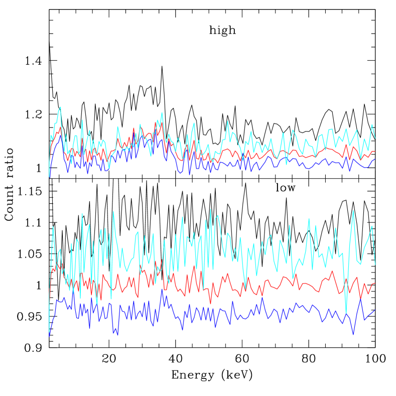
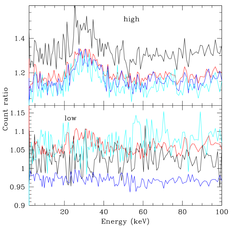
Figure 13: The ratio of spectrum during different times of background observation with respect to that during a ‘low’ orbit for LAXPC20. The left panel shows the result for February 2017 background observation, while the right panel shows that for September 2020 observation. The red line in top panels show the ratio averaged over ‘high’ orbit, while that in the bottom panel shows the ratio for entire observation, including all orbits. The black lines show the ratio during the first 600 s of the orbit, the cyan line shows that during the last 600 s, while the blue line shows that during the middle part of the orbit.

During an orbit the counts are generally minimum in between the two SAA passages and tends to increase as the satellite approaches the SAA, as well as when it exits the SAA. However, the magnitude of variation near SAA passage is more complex. In general, for orbits where the counts are near maximum in the diurnal trend, the counts have a sharp spike as the satellite exits the SAA, while the spike when it approaches the SAA is of much smaller magnitude. On the other hand, for orbits where the counts are near minimum of the diurnal trend, the two branches, towards the entry to SAA and while exiting the SAA are comparable in magnitude. It is possible to avoid some of these artefacts by cutting off the interval surrounding the SAA passage from GTI. However, the software does not implement this as it can reduce the exposure time significantly, which may not be desirable in some studies, e.g., study of bursts. For more sensitive studies it may be advisable to remove 600 s on either side of SAA from the GTI.

All these figures only show the total background count rate, but the spectrum does not simply scale by this rate and hence to look for the variation in the background spectrum, we selected the background observations during February 2017 and September 2020 and calculated the spectrum during a few parts of the observation. For reference, we use the spectrum obtained during an orbit when the count rate was close to the minimum (referred to as ‘low’) of diurnal variation, and choose another orbit when the count rate was close to maximum (referred to as ‘high’). Here the orbit is defined as the period between two consecutive passages through SAA. Figure 13 shows the ratio of counts in the spectrum with respect to the average spectrum during the ‘low’ orbit. The red curve in the top panel shows the ratio when spectrum is averaged over the entire ‘high’ orbit, while the red curve in the bottom panel shows the ratio when the spectrum is averaged over the entire observation covering all orbits. The black lines show the spectrum during the first 600 s of the orbit just after the satellite comes out of SAA. The cyan line shows the ratio when the spectrum is taken over the last 600 s before the satellite enters the SAA, while the blue line shows the ratio for spectrum during the middle part of the orbit, leaving out 900 s on both sides. The left panel shows the results for February 2017 observations, while the right panel shows that during September 2020. It can be seen that during the ‘low’ orbit the difference is generally within 10%. However, during the ‘high’ orbit all curves show a higher ratio and also show a peak around 30 keV which is the Xe K X-ray energy. Further, during the initial part of the orbit the flux is much higher at all energies with the maximum difference exceeding 50% for September 2020 observation. We have checked that even if we restrict to first 300 s of the orbit the ratio is only sightly higher. Further, for ‘high’ orbit the blue and cyan curves are close, indicating that there is not much difference in the spectrum as the satellite enters the SAA. On the other hand, for ‘low’ orbit the counts increase as the satellite is about to enter the SAA region. It turns out that the ‘high’ orbits are the ones where the passage through SAA occurs when the satellite is near the south end of its range. Although, the result is not shown, the ratio of the spectrum during the two ‘low’ orbits is roughly consistent with the expected ratio from Figure 10 except for a peak around 30 keV. We have also looked at similar ratio using individual layers of the detector and the behaviour is similar to that in Figure 13. However, the count rate in the top layer is about twice that in other layers. Hence, the additional counts are larger in the top layer as compared to other layers. Since the additional counts are larger after exit from SAA, some of these could be due to induced radioactivity, while there could be additional contribution from charged particles coming through the collimator. Thus it is clear that there is a significant change in the background spectrum during later times and most of the increase in background appears to be during ‘high’ orbits and for energy around 30 keV.

Figure 14: The residuals in the fit to background of LAXPC20 for the two background observations obtained using the background model described by Antia et al. (2017). The left panel shows the residuals in the light curve with a time-bin of 32 s, while the right panel shows the residuals in the energy spectrum.

Figure 15: The residuals in the fit to background for the two background observations obtained using the background model for faint sources described by Misra et al. (2020) which uses only the top layer of the detector. The top panels shows the residuals in the light curve with a time-bin of 100 s, while the bottom panels shows the residuals in the energy spectrum. The left panels show the results for February 2017 background observation while the right panels show the same for September 2020 observations.

The background model used in the software does account for the increase in the count rate during the ‘high’ orbit to a large extent, but the spectrum is scaled to the average counts and hence is likely to introduce a bump around 30 keV. Typical rms deviations in the fit to count rate are 10 s^-1 when total counts in all anodes are considered. For top layer in 3–20 keV energy range this drops to about 1 s^-1, which is comparable to statistical error for a time-bin of 32 s, used in these fits. This may be expected as the deviations are more prominent in energies above 20 keV. Figure 15 shows the residuals in the background fit for the two observations described above using the background model described by Antia et al. (2017). It can be seen that for the restricted energy range using only top layer, the residuals are roughly consistent with the statistical errors, except for the high orbits during November 2020 observations. However, when all events are considered the background model has significant residuals. Thus it is clear that for faint sources it would be advisable to consider only top layer of the detector with restricted energy range. Figure 15 shows the residuals in the background fit for the same two observations using the background model for faint sources described by Misra et al. (2020) which uses only the top layer of the detector.

Since the background model performs better when only top layer of the detector at low energies is used, it is advisable to use this option for faint sources. This is justified as at low energies a large fraction of counts are registered in the top layers. Figure 16 shows the energy dependence of relative fraction of events in top layer (Anodes 1 and 2) and the top two layers (Anodes 1 to 4) as compared to all layers (Anodes 1 to 7). It can be seen that up to about 10 keV, almost all events are registered in the top layer. Even at 20 keV about 50% of events are registered in the top layer and about 75% in the first two layers. Thus for studies at low energies it is advisable to use only the top layer of the detector, as it reduces the background. An alternative is to drop the data during the ‘high’ orbits to avoid this contamination. This would reduce the duty cycle of the observations and if the observation is for a short duration, the entire part may be during the ‘high’ orbits. The fluctuations in the background determine the sensitivity of LAXPC for faint sources, as discussed in the next section.

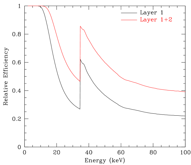
Figure 16: The relative efficiency of only top layer and the top two layers of LAXPC detector as compared to when all layers are used.

Figure 17: The light curve during geomagnetic storms on on September 8, 2017 (left panel) and May 28, 2017 (right panel). The red points show the part of the light curve which would be outside the GTI.

Since the detector background increases close to SAA passage, the contribution is most likely from the flux of charged particles. Although, the detector has veto anode and shield on three sides to protect from charged particles entering from these sides. On the two smaller faces there is only a shield which would offer some protection. However, on the top side there is no veto layer or shield, unlike that in RXTE/PCA which had a propane layer (Jahoda et al. 2006). As a result, there is little protection other than a thin Mylar window, against charged particle coming from the top along the collimator. The opening angle of collimator is about $1^{\circ}$ which gives a solid angle of about 0.0003 st. Thus even for a flux of 1 particle cm^-2 s^-1 st^-1, the detector with an effective area of 2000 cm² would record 0.6 event per s. This level of flux is entirely possible even outside SAA, while close to SAA the flux could be larger.

During a geomagnetic storm the charged particle flux goes up and many more counts are recorded. Figure 17 shows the count rate in detectors during two geomagnetic storms on September 8, 2017 ($Kp=8^{+}$) and May 28, 2017 ($Kp=7$). The $Kp$ index in the parentheses gives a measure of strength of geomagnetic storm. The September 8, 2017 event was the strongest so far during the AstroSat operation. The red points marks the time which would be outside the GTI due to normal SAA definition and would not be considered for analysis. Thus it can be seen that geomagnetic storms can yield significant counts near SAA passage. The most affected regions in this case are those where SAA passage occurs during the north end of the range. For weaker storms, the effect will not be easily seen in light-curve as the net increase would be smaller but such storms can be frequent during high activity part of the solar cycle. Even for smaller geomagnetic storms, of the order of 10 c s^-1 can be added before the SAA passages. If such an event occurs during observation of a variable source, it would be almost impossible to separate it out from variation in source counts. Any burst seen close to SAA passage can be suspect and would require further investigation. During the last two years the solar activity has been low and such storms are rare, but in the coming year the solar activity is likely to pick up and more such events would be seen.

4 Detector Sensitivity and Limitations

There is no difficulty in studying bright sources. The flux limit for faint sources is determined by the fluctuations in the detector background and ability of background model to match these variations. Even for long observations where the spectrum is averaged over a long time, the intrinsic variations in background cannot be modelled satisfactorily and it limits the sensitivity of the detector for faint sources. From the discussion in the previous section we can see that at least, a few counts per second from the source would be required to get any meaningful results. The actual limit would obviously depend on the level of details that need to be studied and the fluctuation in background during actual observation. The Crab observation yields a count rate of about 3000 s^-1 in each detector, which gives a sensitivity limit of about 1 mCrab for faint sources that can be studied. For reference, low energy flux of about $10^{-11}$ erg cm^-2 s^-1 gives a count rate of 1 s^-1. The same difficulty arises even for relatively bright sources at high energies where the count rate can be much less than that in the background. The upper limit on energy to which the spectrum can be studied depends on the source and the extent of details that are required. In the following subsections we illustrate some limitations and capabilities of LAXPC for studying different properties of X-ray sources. Instead of giving limit on flux etc., we illustrate the capabilities and limitations by giving some examples. All the results presented in this section are obtained using the software described in Section 5.2 with default parameters, except for choice of energy range and anodes as specified.

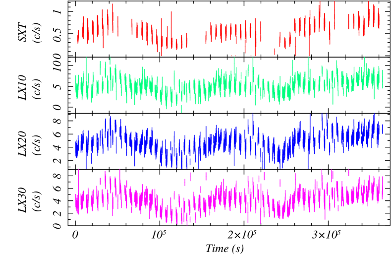
Figure 18: The light curve of NGC 4593 during the AstroSat observation starting on July 14, 2017 in SXT and the three LAXPC detectors with a time-bin of 100 s.

Figure 19: The Cross-correlation between SXT and LAXPC20 light-curve of NGC 4593 is shown as a function of time delay. The red line shows the fit with 2 Gaussians.

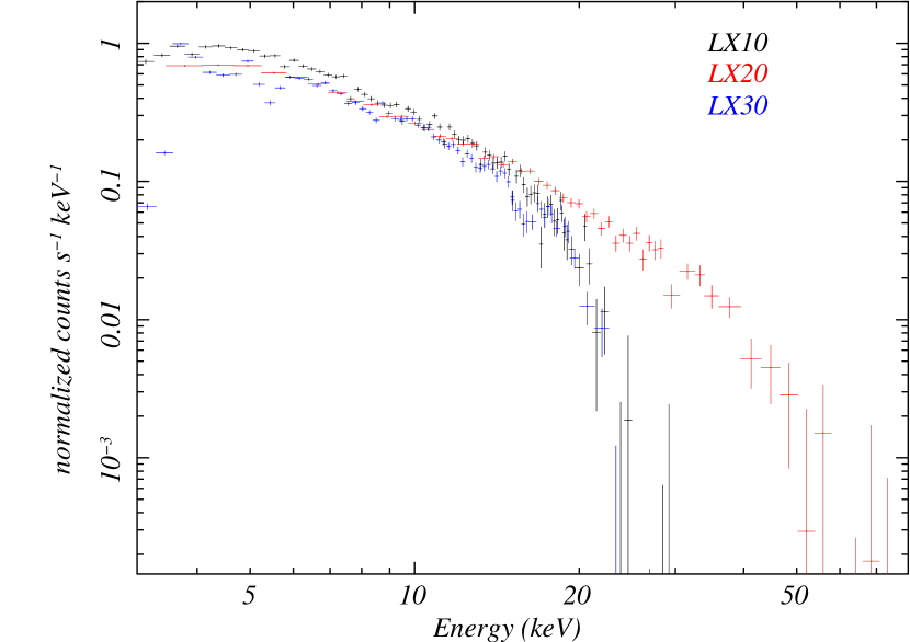
Figure 20: The spectrum of NGC 4593 during the AstroSat observation starting on July 14, 2017 in the three LAXPC detectors.

Figure 21: The fit to the combined spectrum from SXT and LAXPC20 for NGC 4593 is shown with the bottom panel showing the residuals.

4.1 Light Curve and Spectrum

For faint sources typically most flux is observed at low energies and it is better to use only the top-layer of the detector and further restrict the energy range to 3–20 keV. This reduces the background counts by a factor of 10, thus improving the signal to noise ratio. To illustrate the limitation we have selected an AstroSat observation of an Active Galactic Nuclei (AGN), NGC 4593, on July 14, 2016. Figure 18 shows the LAXPC light-curve using only top layer and energy range of 3–20 keV. This source shows a count rate of about 5 s^-1 in all three detectors. For comparison the light curve at low energies from the SXT instrument is also shown. All light curves are with a time-bin of 100 s to reduce the statistical error. It can be seen that all LAXPC detectors and the SXT instrument show similar variation. The SXT being an imaging instrument has low background and further it operates at lower energy of 0.3–10 keV, where the flux is larger. Hence, it is expected to give reliable light-curve for this source. The cross correlation function crosscor of HEASoft v 6.28 tool was used to estimate the time lag between the LAXPC20 (3–20 keV) and SXT (0.5–3.0) keV which is shown in Figure 19. A standard plot of cross-correlation versus time delay was generated using these energy bands with time resolution of 99.86 s with 512 intervals. Two Gaussian models were fitted to the cross-correlation to evaluate the time lag. The resulting fit shows a clear time delay of about 400 s indicating that hard photons lag behind the soft photons (Brenneman et al. 2007).

Figure 20 shows the spectrum observed in each of the LAXPC detectors. There is a reasonable agreement between the three detectors at low energies. The LAXPC20 spectrum continues at high energy also, probably because the background is more reliably estimated. To test the spectrum, the combined spectrum from SXT and LAXPC20 covering 0.5–80 keV was fitted using Xspec to the model phabs*(diskbb + gaussian + powerlaw) and the resulting fit is shown in Figure 21. The model fit yielded a reduced chi-squared of 1.45 (639/442) with 1.5% systematics. Also, significant residuals were seen in the 10–30 keV range, which might be due to a broad reflection component. The disk temperature ($T_{in}$) and photon index ($\Gamma$) obtained were $0.13\pm 0.01$ keV and $1.56\pm 0.01$, respectively, which are consistent with the results of Ursini et al. (2016).

4.2 Pulsation

Several X-ray pulsars have been studied by LAXPC and in general there is no difficulty in estimating the frequency and spin-up rate if the change in frequency is significant. To illustrate the performance, we consider the AstroSat observation of SMC X-2 on May 7, 2020 (ID 20200507_T03_205T01_9000003652), when the average count rate from the source was 2.1 s^-1. Nevertheless, it was possible to estimate the spin period of $2.377441\pm 0.000016$ s at the beginning of observation (MJD 58976.575405) and the spin-up rate of $(3.9\pm 1.1)\times 10^{-11}$ Hz s^-1 using LAXPC20 in single event mode and energy range of 3–20 keV. The resulting pulse profile shown in Figure 22 can be compared with other observations (Li et al. 2016; Jaiswal & Naik 2017). Thus, it is clear that even with a low count rate it is possible to study pulsations.

Figure 22: The pulse profile of SMC X-2 as obtained by LAXPC20 in the energy range 3–20 keV.

Apart from coherent pulsation, LAXPC has been extensively used to study Quasi Periodic Oscillations (QPO) in a wide variety of sources, with frequency ranging from 1 mHz in 4U 0115+63 (Roy et al. 2019) to 815 Hz in 4U 1907+09 (Verdhan Chauhan et al. 2017). The only problem with detecting QPO arises if their frequency is close to the orbital frequency of AstroSat ($\sim 0.15$ mHz) or its harmonics. Up to 10 harmonics of orbital frequency can be easily seen in the power density spectrum and need to be accounted for while identifying QPO frequencies. Similarly, for X-ray pulsars there can be interference from pulse frequencies or its harmonics. But this can be easily removed by modelling the pulse including harmonics and removing their contribution, e.g., for GRO J2058+42 (Mukerjee et al. 2020a).

4.3 Cyclotron Resonant Scattering Features

Detection and studies of Cyclotron Resonant Scattering Features (CRSF) has always been of great interest for direct measurements of magnetic field of the neutron stars and to understand structure of the line forming regions in the accretion column in X-ray binary pulsars. The LAXPC instrument was designed to study CRSF in X-ray pulsars in binaries, as one of its important defined objectives with superior detection efficiency along with its high time resolution capabilities covering 3–80 keV wide energy band. Detection of CRSF requires accurate spectral response and a well defined continuum model which enables detection of absorption features in the source spectrum due to CRSF. For a genuine detection of absorption features in the spectrum and to minimise the possibility of false detection due to any unknown discrepancy of spectral response over entire energy band, one can cross verify and re-confirm presence of these absorption features indirectly by comparing the ratio of source spectrum to that of the well known Crab spectrum having well calibrated power-law spectrum (e.g., Mukerjee et al. 2020a). One can also quantify energy non-linearity, if present, in the spectral response by analysing the Crab ratio plot from known CRSF sources. The LAXPC spectral response were generated carefully by appropriately modelling and accounting for 30 keV florescence photons produced due to Xe K shell interaction of incident X-rays. However, some feature around 30 keV is still seen in most spectra which can interfere with detection of CRSF. Nevertheless, LAXPC, has detected CRSF in many X-ray pulsars such as in GRO J2058+42 (Mukerjee et al. 2020a), Her X-1 (Bala et al. 2020) and Cep X-4 (Mukerjee et al. 2020b) with energies in 30–40 keV region. As an example of detection capability of LAXPC at the highest energy, we attempt to study CRSF in GRO J1008–57, where such feature has been detected at 90 keV (Ge et al. 2020). We used AstroSat observation of this source on November 7, 2017 with exposure time of 43 ks to investigate CRSF at such a high energy close to the ULD of LAXPC20.

Figure 23: The fit to LAXPC20 spectrum of GRO J1008–57 including CRSF at 61 and 84.4 keV with the ratio of the data and fitted model shown in the lower panel. The position of 61 keV feature is marked by an arrow.

Figure 23 shows a fit to the GRO J1008-57 spectrum derived from AstroSat observation. The spectral data was reasonably defined by the combined model defined as phabs(gaussian+powerlaw)highecut*2gabs. The ratio of the data and the fitted model is also shown below for clarity. The power-law with high energy cut-off model defines the continuum reasonably well with parameter values derived which is typical for an X-ray binary pulsar. The hydrogen column density value was frozen at $n_{H}=1.22\times 10^{22}$ cm^-2 as calculated using HEASARC tool for the source. The well known Fe-line emission was detected and its energy and width were fixed during the fit at 6.5 keV and 0.3 keV, respectively. The photon-index was found to be $1.13^{+0.40}_{-0.07}$, E-cutoff at $7.96^{+0.75}_{-0.83}$ keV and E-fold at $26.65^{+0.78}_{-0.79}$ keV. The centroid energy of CRSF was detected at $84.4^{+7.3}_{-4.0}$ keV with the line-depth of $10.1^{+5.2}_{-4.4}$, while the width was frozen at 5.5 keV to constrain its upper limit within ULD. The reduced $\chi^{2}$ of the model fit was 1.6 for 128 degrees of freedom. A systematic error of 2.5% was added to account for uncertainties in the response. The CRSF is thus detected with a significance of about $3\sigma$. Even though this energy is near the upper limit of the nominal range of LAXPC, it turns out that the ULD in LAXPC20 is around 100 keV and hence an absorption feature could be seen in the spectrum around 85 keV. The presence of this feature was also cross verified in the spectral ratio with Crab spectrum. The detected CRSF energy is within the error limit of that reported by Ge et al. (2020). Interestingly, in the AstroSat spectrum, an additional absorption feature was also detected around $61.2^{+1.7}_{-1.5}$ keV which has not been reported earlier.

4.4 Source Contamination

A major problem with LAXPC is its large field of view, with FWHM of about $1^{\circ}$ (Antia et al. 2017), which allows multiple sources in the field of view. If the contaminating source has an angular offset of $30^{\prime}$, then its flux would be reduced by about half, which can give significant contamination depending on relative flux from the two sources. Even at an offset of $1^{\circ}$, 5% of the flux may be registered in LAXPC instrument, a part of which may be attributed to the leakage of higher energy ($>50$ keV) photons through the collimator. A test of this is provided by slew observations, where many known sources are seen through a bump in the light curve. There have been cases when the source was clearly visible even when the offset was $65^{\prime}$. For example, during the slew observation on May 7, 2019, the light-curve in LAXPC20 (Figure 24) shows two clear peaks. The first peak with additional counts of 300 s^-1 is due to GX 5–1 which had an offset of $51^{\prime}$. This source has been observed several times by AstroSat and typical count rate is about 3000 s^-1, thus it appears that about 10% of flux is registered at this offset. The second peak with height of about 100 s^-1 is due to GX 9+1 which had an offset of $62^{\prime}$. This source has also been observed twice by AstroSat with a count rate of about 1800 s^-1. Thus even at this offset about 5% of flux is registered. Hence it is recommended that ideally there should be no significant source within $75^{\prime}$ of the target source.

Figure 24: The light curve during a slew operation on May 7, 2019. The two peaks in the light curve are due to GX 5–1 (offset $51^{\prime}$) and GX 9+1 (offset $62^{\prime}$).

Some well known examples of sources affected by contamination are GRS 1758–258, 4U 1630–472 and IGR J17091-3624. For GRS 1758–258 there is another source, GX 5–1, $40^{\prime}$ away, which is more than 10 times brighter. As a result, the contaminating source overwhelms the target. Even if the observation is made with an offset of $30^{\prime}$ on the opposite side, GX 5–1 can still contribute 5% of its on-axis flux which would be comparable to 50% of the GRS 1758–258 flux. Thus it is difficult to study this source using LAXPC. Further, with such offset the target would be outside the field of view of the SXT and hence it would not be possible to do broadband spectral studies. Similarly, 4U 1630–472 has contamination from AX J1631.9–4752 which is $35^{\prime}$ away. In this case, both sources have comparable flux and it may be possible to subtract the contribution from contaminating source (Baby et al. 2020). The 1310 s pulsation from the contaminating source were used to estimate its flux. There are a few other sources also in the field of view, but they are probably transients and may not be in outburst at the time of observation. But this needs to be checked. For IGR J17091–3624, there is a contamination from GX 349+2, $40^{\prime}$ away, which could be a few times brighter than the target. It may be possible to remove the contamination, if simultaneous observation of the contaminating source are available from other instruments, or an estimate of flux is available from monitoring instruments like, MAXI or Swift/BAT (Katoch et al. 2020).

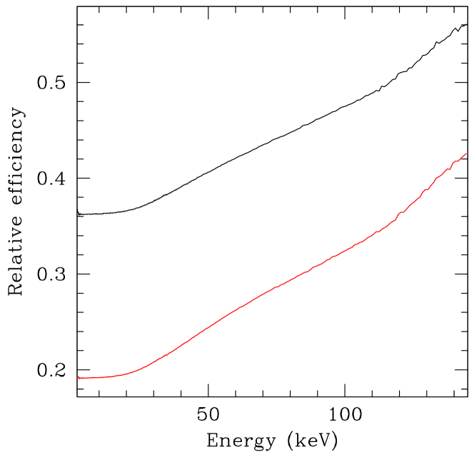
Figure 25: The relative efficiency of LAXPC20 detector with offset of $30^{\prime}$ (black line) and $40^{\prime}$ (red line) as compared to on-axis response.

To remove the contamination, the contaminating source needs to be modelled and a response with offset needs to be used to calculate its contribution to the observed spectrum. The responses with offset have been calculated for LAXPC20. Figure 25 shows the relative efficiency of LAXPC20 for offset of $30^{\prime}$ and $40^{\prime}$ with respect to on axis response. It can be seen that although at low energy the efficiency can be somewhat low, it increases with energy. These responses have been averaged over a circle with a given offset. There would be some dependence on the angle with respect to detector side. The efficiency would be higher when the source is at the same offset along the diagonal of the collimator cells, as compared to that along the side. This is not accounted for as it is not possible to specify this angle during pointing.

Figure 26: The light curve during a slew observation on August 8, 2019 is shown in the left panel. The right panel shows the fit to the spectrum of the possible transient source taken over the duration of the peak in the light curve.

4.5 Possible Detection of a New Transient

LAXPC can be used to scan the sky for new sources. Although, the pre-planned scan has not been attempted so far, between two observations the satellite slews from one source to another and this is similar to a scan. All slew observations have been analysed and during one of these observations on August 8, 2019 a peak was seen in the light curve around 13:13 UTC when the instrument was pointing at RA 288.717 and Dec 17.367. Figure 26 shows the light curve for the observation and the source spectrum taken during the peak. The spectrum was fitted to a powerlaw form with a systematics of 1%. The resulting fit (Figure 26) with a reduced $\chi^{2}$ of 1.2 yielded the index of $1.67\pm 0.09$. A ToO to observe this region was proposed and the observation was carried out on August 15, 2019, but no signal was seen during that observation.

5 Analysis Software

Three different software are available to process the level-1 data to obtain science products. These are LAXPClevel2DataPipeline (Section 5.1) written in C++ and LaxpcSoft written in Fortran. The latter includes two related software, the basic software includes two Fortran programs, laxpcl1 and backshift developed by TIFR team (Section 5.2) and a suite of Fortran programs based on the basic programs for different tasks developed by the AstroSat Science Support Cell at IUCAA (Section 5.3). These are described in the following subsections.

5.1 LAXPClevel2DataPipeline

The LAXPC Level-2 data pipeline version 3.1 was developed with support from ISRO Space Applications Centre (SAC), Ahmedabad. The pipeline works on the level-1 data downloaded from the Indian Space Science Data Centre (ISSDC) archive. The pipeline generates various level-2 output data files for the scientific studies and other ancillary files which are inherited from the level-1 data in FITS format. Before producing these files, the pipeline checks for the data frame sequence order, duplicate frames or possible frame corruption during data transfer. If needed, the data frames are reordered. The level-2 files generated for the scientific studies are : event file, Good Time Interval (GTI) file, lightcurve file and spectrum file. The other ancillary files inherited from the level-1 are : Time Calibration Table (TCT) file, Make Filter (MKF) file giving information about the satellite position etc., Low Bitrate Telemetry (LBT) house-keeping file, orbit file and attitude file. Additionally, the pipeline also has independent routines to reprocess the lightcurve and spectrum which can be generated as per requirements. Currently, this pipeline has only limited support.

5.2 laxpcl1 and backshift

These are two standalone Fortran programs to process the level-1 data that are available from the AstroSat archives. The readme files with the package give the detailed instructions for usage. The tar file also includes the background files required for all background observations. While the detector response files for all detectors are available from the LAXPC website. The level-1 inputs required includes the Event Analysis (EA) mode files which give the record of each event that is detected and Broad Band counting (BB) mode files giving the counts of various categories of events in a predefined time-bin. Apart from these, the .mkf file giving the orbital and pointing parameters and the time calibration table (tct) file giving the conversion from instrument time to UTC are also required. These programs can handle data from multiple orbits after removing the overlapping part of data between consecutive orbits, but treat each detector independently. This program also corrects for problems with frame sequence ordering as well as event time ordering. The program also gives a statistics of the data processed, including the total exposure, fraction of gaps in data and frame-loss that has been detected. In most observations the frame-loss is less than 0.1%, but in some cases it can be a few percent or more. In such cases it may be necessary to discard the time intervals with large frame-loss. Orbit-wise statistics of frame-loss is available in ‘.frame’ file, which can be listed using ‘grep Frame lxp2level2.frame’.

The program laxpcl1 is the main routine which generates the light curve, spectrum, event file and GTI file giving the list of GTIs. All output files are in both ASCII and FITS format. It also generates the background spectrum and light curve using the background model to estimate the background contribution. A FITS file giving orbital parameters as required by the tool as1bary to apply the barycentric corrections to time is also generated. The channel range and anodes to be used can be specified. To suppress some oscillations in spectrum, two channels are binned together for LAXPC10 and LAXPC30, while for LAXPC20, four channels are binned. Thus the original spectrum in 1024 channels is reduced to 512 or 256 channels. However, this binning is done at the end and the input channel range to be specified to laxpcl1 is in the full range of 0–1023. This should be accounted for while specifying the input. The events in event file are of two types, single events, where all energy is deposited in one anode, and double events, where the energy is deposited in two anodes, of which at least, one energy is in Xe K X-ray range. There is an option to exclude double events. This may be useful in some cases as the response is better defined for these, though the efficiency may be reduced to some extent (Antia et al. 2017). Since the ULD threshold is applied to each anode separately, the double events can have energies exceeding ULD and in principle, it is possible to study the spectrum up to about 110 keV, and these are included in the response files. However, the efficiency of detector is very low for these events. Since the event files can be large, there is an option to suppress writing these files. This program generally requires two passes, one to generate the GTI list and another to do the calculations using this GTI file, which could be edited to choose any subset of intervals. To generate the GTI file it is advised to use a time-bin of at least 1 s. The final light curve can be generated for any time-bin, though there is some limit on dimension which may truncate the light curve when very small time-bin is used. If the GTI file is already available then only one pass through laxpcl1 is needed.

The program backshift is used to account for gain shift between the source and background observation after running laxpcl1. It uses the log of gain to estimate the shift in gain and corrects the background spectrum to match the gain during source observation. The correction is applied both to the background spectrum and light curve. The background observation to be used has to be specified in an input file for laxpcl1. In general, the background observation closest in time to source observation is to be used and backshift gives recommendations about which background file can be used. It also gives recommendation about which response file has to be used to fit the spectrum. There are four sets of response files, the default is for all events and anodes. This may be the name that is recommended by backshift. Other set of responses are for single event mode with ‘SE’ in the name. The remaining two sets are for only the top layer, ‘L1’ and ‘L1SE’ for all events and only single events, respectively. There is also an option to remove diurnal variation in the light curve, which would not affect the spectrum. For LAXPC30, response files are available for different densities and the program also recommends which response needs to be used. In some cases, neighbouring density may also be tried. For LAXPC20, the program also recommends the value of offset that may be used in the gain fit while fitting the spectrum. The offset may be frozen to this value (and slope to 1.0) if there is a difficulty in estimating the gain parameters using gain fit.

For faint sources or sources with soft spectrum, it may be advisable to use the single event mode with energy restricted to 3–20 keV. For this the option $\mbox{\tt ian}=1$ (for top layer), $\mbox{\tt nul}=-2$ (to apply background fit for top layer) and $\mbox{\tt iev}=1$ or $-1$ (for selecting single events only) should be used. The energy range to be used can depend on the source.

5.3 Software with Individual Routines

A wrap around software to the primary one described above has been developed for ease of certain kind of analysis of LAXPC data. The software can be obtained from the AstroSat Science Support Cell web-page . Details of the software and instructions for use are given in README files included in the software. Here we outline some of the basic highlights and the functionality of the software.

The software can produce a combined merged clean event file (typically called level2.event.fits) for all three LAXPC units which is time sorted, allowing for ease of timing analysis. Apart from Time, the other columns of the event file are Layer number, LAXPC unit, Channel and Energy. The Energy of the event is estimated using the channel to energy conversion from the appropriate response file. This allows the user to make appropriate selections, either using the ftools command fselect, or by using the other routines of the software. The Event file also contains as separate data unit, the appropriate names of the response files for the three LAXPC units as a function of time for the observation.

A number of individual routines are provided which can run from the command line with flags as inputs. Hence they allow for easy customized scripting by the user. The spectra and lightcurves generated are compatible with high level HEASoft tools such as powspec, lcurve, Xspec, crosscor etc. The individual routines can be used to obtain:

1. A Good Time Interval (GTI) file that takes into account earth occult and SAA passage.

2. A merged orbit file that is required to make Barycentric corrections.

3. Lightcurves at a given time-bin for user specified multiple energy bands with a GTI file as a input. Lightcurves can be generated for different combination of the LAXPC units and for all layers or only for the first layer.

4. Spectra for each of the three units for the input GTI file. Spectra can be generated for all layers or only for the first layer. Appropriate response files are copied from the software database to the working directory and the ‘RESPFILE’ keyword in the spectra files is updated.

5. Estimated background spectra for each LAXPC for the input GTI file. The background estimation can be done either based on blank sky observations closest to data or gain. All or first layer can be chosen. The ‘BACKFILE’ keyword in the spectra file is changed to the resultant background file.

6. Estimated background lightcurve corresponding to the extracted lightcurve.

7. GTI file for providing the time intervals when the flux given in an input lightcurve is within some user specified values. This is useful to generate flux resolved spectroscopy.

8. Time-lag, fractional r.m.s, coherence and intrinsic coherence as a function of both frequency and energy. These are computed directly from the event file rather than lightcurves and hence is computationally efficient when performing high frequency analysis. The routine also provides the power spectrum along with the dead-time corrected Poisson level. A subsidiary routine rebins the power spectrum and converts it into Xspec readable format, which allows the user to fit the power spectrum using Xspec models and flexibility.

9. Dynamic Power spectra which are power spectra computed for consecutive time intervals. This is useful to see the rapid variation in Quasi-periodic oscillation (QPO) frequency.

10. Estimate of background spectra and lightcurve using an alternate method applicable for faint sources as described by Misra et al. (2020).

6 Science Goals of LAXPC Instrument: Status of their Realisation so Far

AstroSat was conceived as a multiwavelength observatory for simultaneous observations of galactic and extragalactic sources in Visible, UV and X-ray bands using a suite of four co-aligned instruments for studies of different classes of galactic and extragalactic objects. Three co-aligned X-ray instruments, sensitive in the X-ray energy region 0.5–150 keV were designed to investigate temporal and spectral characteristics of the sources to elucidate their nature and probe the complex radiation process operating in them.

The LAXPC instrument was designed to measure the intensity variations of bright X-ray sources over a wide time scale, from 0.1 ms to minutes, days and months. The X-ray binaries, with a neutron star or a black hole as the compact object, were special targets for the LAXPC studies, as they exhibit a range of periodic and aperiodic variations on almost all time scales. Accurate determination of continuum energy spectra of X-ray binaries to decipher the dominant radiation processes as well as to search for the presence of weak spectral features known as Cyclotron lines that provide a measurement of the magnetic field of the neutron star, is another major objective of LAXPC. To achieve these objectives, LAXPC tags the arrival time of every detected photon with an accuracy of 10 $\mu$s and also achieves a moderate energy resolution over the entire range of 3–80 keV.

In this section we demonstrate how the various science goals of LAXPC instrument have been met by giving some representative examples in each case. More detailed discussion of scientific result is covered by Yadav et al. (2020). The LAXPC instrument was designed with the following objectives (Agrawal et al. 2017):

1. Detailed studies of stellar-mass and supermassive black holes: Several black hole sources in both mass ranges have been studied. For example, using the combined SXT and LAXPC spectrum, Mudambi et al. (2020) have derived the spin of the black hole in LMC X-1. Similarly, Pahari et al. (2018) and Sridhar et al. (2019) have estimated the mass and spin of black holes in 4U 1630–472 and MAXI J1535–571.An example of a study of supermassive black hole is the blazar RGB J0710+591 by Goswami et al. (2020) using the multiwavelength capability of AstroSat by combining data from UVIT, SXT and LAXPC.

2. Studies of periodic (pulsations, binary light curves) variabilities in X-ray sources: The LAXPC instrument with its high time resolution capability is ideally suited to measure the spin periods of the X-ray pulsars to a high precision and deduce their derivatives. The spin-up or spin-down rates of these pulsars is determined by many factors, including accretion and the magnetic field, which in turn can be studied by the measured changes in the spin period. Amin et al. (2020) measured the spin period and spin-up rate of the neutron star in the LMXB source 3A 1822–371. The shape of the emitted pulse depends on modes of accretion, geometry of accretion column and configuration of its magnetic field with respect to an observer’s line of sight. Therefore, such studies offer insight into the physical processes in the vicinity of the pulsar. For example, Mukerjee et al. (2020a) studied the spectral and timing properties of GRO J2058+42 using data from AstroSat during a rare outburst in April 2019. LAXPC data have been used to study pulsation over a wide range of period from 2.3 ms for a transient accretion powered millisecond X-ray pulsar SAX J1748.9–2021 (Sharma et al. 2020) to 604 s for 4U 1909+07 (Jaiswal et al. 2020). LAXPC is well suited for studying the pulsar period evolution and hopefully more such studies will emerge in the future. LAXPC also offers the possibility of inferring the evolution of the binary period by studying the binary light curve over a long base line of years. Using LAXPC observations of Cyg X-3 covering nearly one year, Pahari et al. (2018) determined the binary orbital period to be $17253.56\pm 0.19$ s.

3. Studies of QPOs and aperiodic variabilities in X-ray sources: LAXPC data have been used to study QPOs in a number of X-ray sources covering a wide range of frequencies. For example, Belloni et al. (2019) and Sreehari et al. (2020) detected a clear HFQPO in well known black hole binary GRS 1915+105, whose frequency varied between 67.4 and 72.3 Hz. A QPO of 90 mHz centroid frequency was detected for the first time by LAXPC in GRO J2058+42 during its rare outburst of 2019 (Mukerjee et al. 2020a). Apart from QPOs, the LAXPC instrument with its high time-resolution also allows the study of the time lag between different energies of X-rays. Because of wide energy coverage these studies can be extended to energies of 30 keV and above. Misra et al. (2017) have analysed LAXPC data from Cyg X-1 in the hard state to derive time lag between Soft (5–10 keV) and Hard (20–30 keV) photons which increase with energy for both the low and high frequency components. The event mode LAXPC data allowed them to perform flux resolved spectral analysis on a time-scale of 1 s, which clearly shows that the photon index increased from 1.72 to 1.80 as the flux increased by nearly a factor of two. Apart from QPO, the neutron star X-ray binaries show thermonuclear X-ray bursts which have also been studied by LAXPC. Verdhan Chauhan et al. (2017) used the LAXPC observation of the LMXB 4U 1728-24 on March 8, 2016 to study a typical Type-1 burst of about 20 sec duration. The dynamical power spectrum of the data in the 3–20 keV band, shows the presence of a burst oscillation whose frequency increased from 361.5 to 363.5 Hz. These results demonstrate the capability of LAXPC instrument for detecting millisecond variability even from short observations. Similarly, Devasia et al. (2021) have studied thermonuclear bursts in Cyg X-2. They have carried out energy resolved burst profile analysis as well as time resolved spectral analysis for each of the 5 bursts that were observed.

4. Low to moderate spectral resolution studies of continuum X-ray emission and CRSF: One of the prime objectives of LAXPC is to measure the continuum energy spectra of Neutron star binaries to a high precision for detecting usually faint signal of the Cyclotron lines. Using the LAXPC observations, Cyclotron lines have been discovered in at least half a dozen pulsars. In section 4.3 detection of CRSF in the spectra of several pulsars observed with the LAXPC, has been discussed demonstrating the LAXPC capability for such investigations. For example, Mukerjee et al. (2020a) carried out a phase resolved study of CRSF in GRO J2058+42, to find significant variation in CRSF energy with pulse phase. Bala et al. (2020) studied secular variation in energy of CRSF in Her X-1 by comparing the result with earlier observations..

5. Search for transient X-ray sources by surveys in a limited region of the galactic plane: So far a systematic survey has not been carried out, but between two science observations the satellite slews from one source to another. The slew data have been scanned for potential sources, but most features were found to be associated with known sources, except for the one instance described in Section 4.5.

The main goals of LAXPC have been realised to a certain extent. However, the detection of new transient sources in limited regions of the galactic plane through a dedicated survey is not yet planned. A large fraction of the LAXPC and SXT data still remains to be analysed. This could be achieved by encouraging and involving more number of students and researchers in data analysis and improving our understanding of calibrations issues pertaining to instrument gain, background, spectral response etc. The phenomenon of kHz QPOs, a major discovery by RXTE in about 15 LMXBs, has not been revisited by AstroSat even though it is ideally suited for this study. The multiwavelength study was a prime objective of AstroSat to understand the relationship between radiation in different bands in the AGNs i.e., is the UV flux from AGNs generated by the reprocessing of X-rays in the accretion disk? In X-ray binaries one measures time lag of hard X-rays with respect to the soft photons to infer if hard X-rays are reflection component due to up scattering of soft photons on the surface of the hot disk. It is hoped that some of these gaps in the AstroSat/LAXPC science results will be addressed in the coming years.

7 Summary

AstroSat has completed five years of operation, during which more than 2000 different pointings and over 1000 distinct sources have been observed. The data for most observations are now available from the AstroSat archive. By now only one of the three detectors, i.e., LAXPC20 is working nominally. The response of detectors is reasonably understood and is stable. The detector background has been increasing with time and some diurnal variations have been seen both in the background and in fitted parameters to source spectrum. The variation in background puts a limit on the source flux of about 1 mCrab, below which it would be difficult to study the source. Even at this limiting flux it is possible to fit the spectrum to a reasonable extent and to study pulsations. LAXPC has successfully detected CRSF in several sources. The detection of these features can be confirmed by looking at the ratio of source to the Crab spectrum.

To account for drift in the gain of detectors, it is recommended to use gain fit in Xspec while fitting the spectrum, even when the recommended response is used. The fitted slope and offset should be compared with the values shown in Section 2.3 to check that the correction is in a reasonable range. Significantly different values would imply that gain fit has fitted some other spectral variation. In such cases the slope should be fixed at 1 and the offset should be fixed at the value recommended by backshiftv3. A few observations may have a significant frame-loss during data transmission and it may be necessary to discard the data during these time intervals. For faint sources it is advisable to use only the top layer of the detector to reduce the background. Because of a relatively large field of view, there is a possibility of another source in the field of view and this should be checked before analysing the LAXPC data.

Many X-ray sources have been studied using LAXPC data resulting in more than 40 publications. The scientific results are summarised in a companion paper (Yadav et al. 2020).

References

- [1] Agrawal, P. C. 2006, AdSpR, 38, 2989.
- [2] Agrawal, P. C., Yadav, J. S., Antia, H. M., et al., 2017, JApA, 38, 30
- [3] Amin, N., Roy, J., Chakroborty, S., et al. 2020, JApA (this volume)
- [4] Antia, H. M., Yadav, J. S., Agrawal, P. C., et al. 2017, ApJS, 231, 10
- [5] Antia, H. M., Katoch, T., Shah, P., Dedhia, D., Gupta, S., Gaikwad, R., Sharma, V., Vibhute, A., Bhattacharya, D. 2020a, GCN 27313
- [6] Antia, H. M., Katoch, T., Shah, P., Dedhia, 2020b, GCN 27313
- [7] Baby, B. E., Agrawal, V. K., Ramadevi, M. C., et al. 2020, MNRAS, 497, 1197
- [8] Bala, S., Bhattacharya, D., Staubert, R. and Maitra, C. 2020, MNRAS, 497, 1029
- [9] Belloni, T. M., Bhattacharya, D., Caccese, P., Bhalerao, V., Vadawale, S., Yadav, J. S. 2020, MNRAS, 489, 1037
- [10] Bhalerao, V., Bhattacharya, D., Vibhute, A. et al. 2017, JApA, 38, 31
- [11] Brenneman, L. W., Raynolds, C. S., Wims, J., and Kaiser, M. E. 2007, ApJ, 666, 817
- [12] Devasia, J., Raman, G., Paul, B. 2021, NewA 8301479
- [13] Ge, M. Y., Ji, L., Zhang, S. N., et al. 2020, ApJ 899, L19
- [14] Goswami, P., Sinha, A., Chandra, S. 2020, MNRAS, 492,796
- [15] Jahoda, K., Markwardt, C. B., Radeva, Y., et al. 2006, ApJS, 63, 401
- [16] Jain, C., Paul, B., Dutta, A. 2010, MNRAS, 409, 755
- [17] Jaiswal, G. K., Naik, S. 2017, MNRAS, 461. L97
- [18] Jaiswal, G. K., Naik, S., Ho, W. C. G., Kumari, N., Epli, P., Vasilopoulos, G. 2020, MNRAS, 498. 4830
- [19] Li, K. L., Hu, C.-P., Lin, L. C. C., Kong, A. K. H. 2016, ApJ, 828, 74
- [20] Katoch, T., Baby, B. E., Nandi, A. et al. 2020, MNRAS (in press) arXiv:2011.13282.
- [21] Misra R., Yadav J. S., Verdhan Chauhan J., et al. 2017, ApJ, 835, 195.
- [22] Misra R., Roy, J., Yadav, J. S. 2020, JApA (this volume)
- [23] Mudambi, S. P., Rao, A., Gudennavar, S. B., Misra, R., Buggly, S. G. 2020, MNRAS, 498, 4404
- [24] Mukerjee, K., Antia, H. M., Katoch, T. 2020a, ApJ, 897, 72
- [25] Mukerjee, K., et al. 2020b, (in preparation)
- [26] Pahari, M., Antia, H. M., Yadav, J. S., et al., 2018, ApJ, 849, 16
- [27] Pahari, M., Bhattacharyya, S., Rao, A. R., et al., 2018, ApJ, 867, 86
- [28] Roy, J., Agrawal, P. C., Iyer, N, K. et al. 2019, ApJ 872, 33
- [29] Sasano, M., Makashima, K., Sakurai, S., Zhang, Z., Enoto, T. 2014, PASJ, 66, 35
- [30] Shaposhnikov, N., Jahoda, K., Markwardt, C., et al. 2012, ApJ, 757, 159
- [31] Sharma, R., Beri, A. Sanna, A., Datta, A. 2020, MNRAS, 492, 4361
- [32] Singh K. P., Tandon S. N., Agrawal P. C., et al. 2014, SPIE, 9144, 1SS.
- [33] Singh K. P., Stewart, F. C., Chandra, S., et al. 2016, SPIE, 9905, 1ES
- [34] Sreehari, H., Ravishankar, B. T., Iyer, N. et al. 2019, MNRAS, 487, 928
- [35] Sreehari, H., Nandi, A., Das, S., et al. 2020, arXiv:2010.03782
- [36] Sridhar, N., Bhattacharyya, S., Chandra, S., Antia, H. M. 2019, MNRAS, 487, 4221
- [37] Tandon, S. N., Hutchings, J. B., Ghosh, S. K. et al. 2017, JApA 38, 28
- [38] Ursini, F., Petrucci, P.-O., Matt, G., et al. 2016, MNRAS, 463, 382
- [39] Verdhan Chauhan, J., Yadav, J. S., Misra, R. et al. 2017, ApJ, 841, 41
- [40] Yadav, J. S., Agrawal, P. C., Antia, H. M., et al. 2016a, SPIE, 9905, 1D.
- [41] Yadav, J. S., Misra, R., Chauhan J. V.,et al. 2016b, ApJ, 833, 27
- [42] Yadav, J. S., Agrawal, P. C., Misra, R., Roy, J., Pahari, M., Manchanda, R. K. 2020, JApA, (this volume)